Symmetry-Adapted Fourier Series for the Wallpaper Groups

1
Departement Fysica, Universiteit Antwerpen, Groenenborgerlaan 171, 2020 Antwerpen, Belgium
2
Institut für Theoretische Physik und Astrophysik, Universität Würzburg, Am Hubland, D-97074 Würzburg, Germany
Symmetry 2012, 4(3), 379-426; https://doi.org/10.3390/sym4030379
Submission received: 11 June 2012
/
Revised: 27 June 2012
/
Accepted: 5 July 2012
/
Published: 17 July 2012
(This article belongs to the Special Issue Crystal Symmetry and Structure)
Abstract
:Two-dimensional (2D) functions with wallpaper group symmetry can be written as Fourier series displaying both translational and point-group symmetry. We elaborate the symmetry-adapted Fourier series for each of the 17 wallpaper groups. The symmetry manifests itself through constraints on and relations between the Fourier coefficients. Visualising the equivalencies of Fourier coefficients by means of discrete 2D maps reveals how direct-space symmetry is transformed into coefficient-space symmetry. Explicit expressions are given for the Fourier series and Fourier coefficient maps of both real and complex functions, readily applicable to the description of the properties of 2D materials like graphene or boron-nitride.
1. Introduction
The central concept for describing the structure of crystalline solids is that of the unit cell, the periodic repetition of which results in a spatially extended crystal exhibiting particular symmetries. For both three- and two-dimensional (3D and 2D) crystals, the enumeration of possible unit cell symmetries was first carried out by E.S. Fedorov at the end of the nineteenth century [1,2,3]. Deriving the possible (3D or 2D) unit cell symmetries requires combining a crystal’s possible point group symmetry operations (rotations, rotation-inversions or reflections leaving one point of the crystal lattice invariant) with translations. It is well known that for three dimensions, this results in 230 so-called “space groups”. For two dimensions, only 17 planar groups, the so-called “wallpaper groups”, are possible. All information on space/wallpaper groups is nowadays collected in the many-volume International Tables for Crystallography [4,5,6,7,8].
The information compiled in the “International Tables” [4,5,6,7,8] is particularly useful for interpreting diffraction experiments: X-ray, neutron, and electron diffraction are the de facto methods for crystal structure determination and provide access not only to a crystal’s space group but also to the contents of its unit cell. In particular, the notion of extinctions (systematic absences of certain types of reflections due to specific symmetries present in the structure) is often fundamental for correctly determining a crystal’s space group.
The crystallinity—in other words, translational periodicity—of a solid is the essential starting-point in solid-state physics. For example, the quantum theory of electrical conductivity, involving Bloch waves, completely relies on the repetition of a unit cell for the concepts of reciprocal space and band structures to be valid (see e.g., [9]). Surprisingly, while the translational periodicity of a solid is used extensively in theory, considerations concerning the unit cell’s symmetry are far less frequently encountered.
Translational symmetry naturally leads to a Fourier series. Submitting a Fourier series to additional symmetry constraints then results in relations between Fourier coefficients, or even in the vanishing of certain terms of the Fourier series. In this paper, we revisit the symmetry-adapted Fourier series for the planar wallpaper groups, and focus on the symmetry pattern formed by equivalent Fourier coefficients in 2D discrete coefficient space. Apart from the explicit expressions for the symmetry-adapted Fourier series and the symmetry relations between Fourier coefficients, we provide visualisations showing how direct-space symmetry is transformed into coefficient-space symmetry.
In the first sections of the paper (Section 2, Section 3 and Section 4) we provide a pedestrian approach to the problem, work out some examples in detail, and make the link with the information contained in the “International Tables” [4,5,6,7,8] used by crystallographers. The bulk of the paper is formed by the 17 tables with detailed information on the Fourier series and Fourier coefficients for each of the wallpaper groups (Section 5). In Section 6, we discuss some points in more detail and summarise our results.
While the paper is hoped to have pedagogical merits, we also strive for completeness and applicability: The information derived is relevant for present-day materials science. For example, graphene [10], a 2D honeycomb network of carbon atoms, is at present one of the most extensively investigated materials. Its equilibrium properties (e.g., electronic density) are expected to display the 2D symmetry of its underlying atomic structure (wallpaper group , see below).
2. Two-Dimensional Translational Symmetry
We consider a scalar function depending on the spatial coordinates of 2D coordinate space; and are the basis vectors of the underlying Cartesian axes system. It is well known that if f is periodic along two linearly independent vectors and , it can be written as a Fourier series
with
where and are obtained from and via
The Fourier coefficients are obtained by integration,
where we have introduced the shorthand notation ; is the area spanned by the vectors and (most generally, and define a parallelogram).
In the context of the planar wallpaper groups, and are of course the (primitive) basis vectors of a Bravais lattice and and the associated reciprocal basis vectors, satisfying the property
For planar space groups, there are only 5 Bravais lattices. Their primitive basis vectors and reciprocal basis vectors are summarized in Table 1.
It is easy to show that for f to be real, the condition
needs to be fulfilled.
3. Full Wallpaper Group Symmetry
In addition to translational symmetry, each wallpaper group (except the group) displays additional symmetry: invariance under rotations, reflections and/or glide reflections. Note that the latter are neither point group nor translational group elements. (The planar crystallographic point groups are 1, 2, m, , 4, , 3, , 6 and [4].) The purpose of the present paper is to derive restrictions on the Fourier coefficients for each of the 16 non- wallpaper groups. Indeed, a specific symmetry requirement (i.e., invariance of f under a certain symmetry operation) must be reflected in Fourier expansion Equation (1), which is only possible by having certain relations between its Fourier coefficients [similar to the reality criterion—Equation (8)].
3.1. Rotations
A rotation over about the origin (or about the “virtual” z-axis) moves a point with coordinates to the point with coordinates
Rotating the function rather than the coordinates results in the transformed function , given by
For f to be invariant by the rotation, one must have , so that
By rewriting the scalar product as
and establishing the relationship between and one obtains the symmetry rule for the coefficients associated with a rotation over .
As an example, let us consider —6-fold rotational symmetry. The matrix reads
and the scalar product is obtained as
where . For a hexagonal lattice—implied by the presence of 6-fold rotational symmetry—we have (see Table 1) and , so that
On the other hand, we have for that
Equating and for arbitrary then leads to the system of equations
from which the dependence follows:
Recalling Equation (11), we have
and since the range of both double summation indices and is the same (), we can write
with given by the inverse relations of Equations (19) and (20):
We can change the notation for the double summation index from to in Equation (22) so that
Since Fourier coefficients are uniquely defined, we arrive at the following property for the coefficients :
Explicitly:
If we perform a second rotation over , the function f remains invariant. Therefore, we can repeat relation Equation (28) and put
Continuing to repeat relation Equation (28) leads to the following sequence of equalities:
It turns out that after six repetitions we are back at , which corresponds to the observation that repeating rotation 6 times is equivalent to the identity operation. Any index pair (excluding ) belongs to a set of 6 equivalent indices that cyclically transform into one another via relation Equation (30).
As a result, a hexagonal Bravais lattice with a 6-fold rotation axis at its center—i.e., the wallpaper group—implies that the scalar function can be written as
where is a domain of integer pairs that contains exactly one of the 6 equivalent pairs of each of the sets of double indices defined via Equation (30).
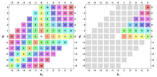
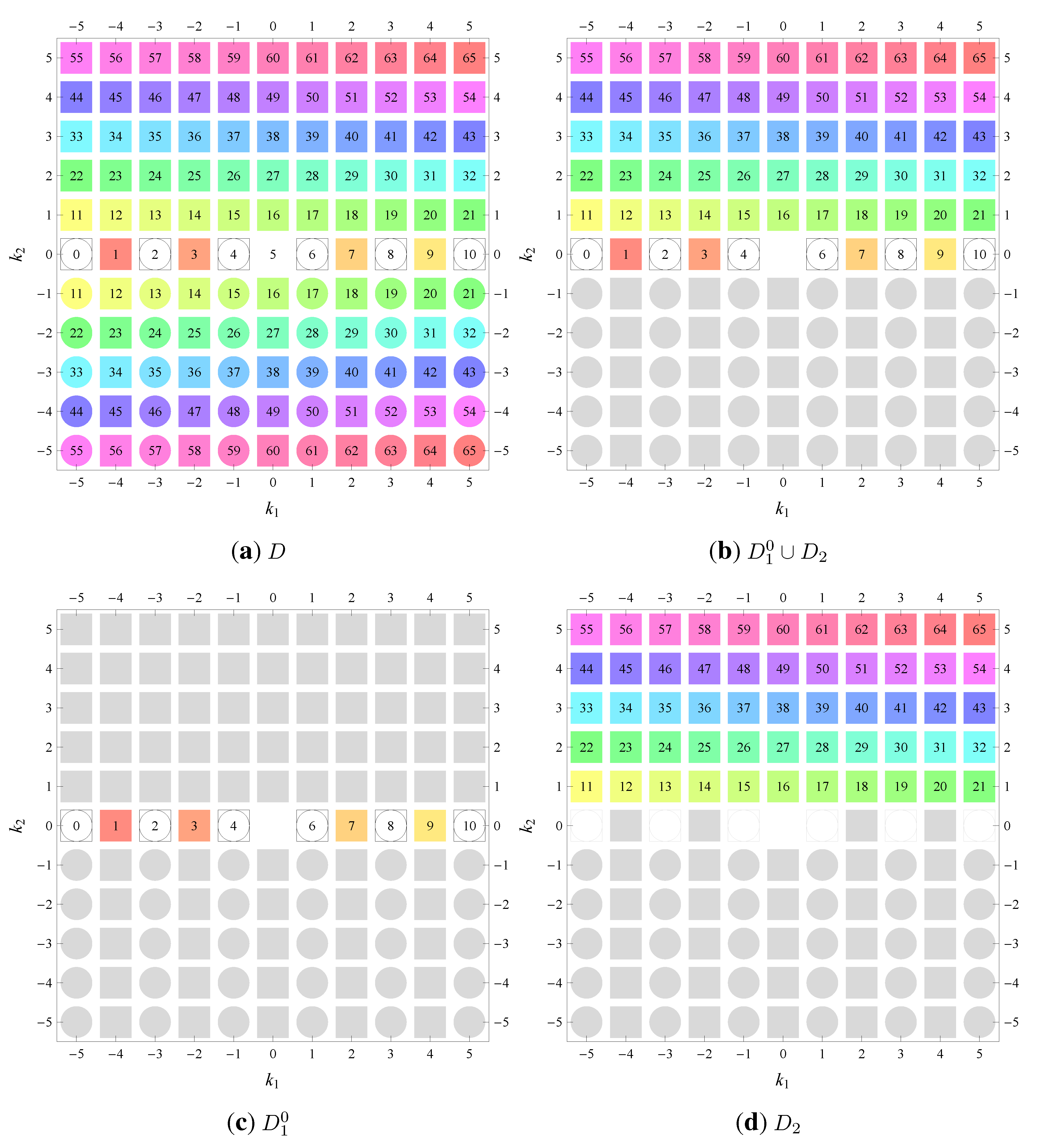
In Figure 1(a) we show the equivalence of points in the range (forming a domain D). The 6 points of each set are represented by squares with a same color and number. One can nicely see how the 6-fold rotational symmetry in coordinate space is mapped onto a “distorted” hexagonal symmetry in index space. Figure 1(b) shows a possible choice of for the numbered points in Figure 1(a); the grey points all have an equivalent representative in the triangle of colored points. The latter can be thought of as a kind of “asymmetric unit” for Fourier coefficients. It is also reminiscent of the so-called “irreducible (wedge of the) Brillouin zone (IBZ)”, a.k.a. “representation domain”, which contains only one vector of each star of in the Brillouin zone (see e.g., [5], Chapter 1.5 and [7], Chapter 2.2.7). Indeed, from knowledge of the values of the Fourier coefficients with indices in the minimal domain , the values of the Fourier coefficients with indices from all coefficient space can be generated by using the symmetry property for Fourier coefficients, Equation (30).
Fourier series Equation (32) can be elaborated into a more explicit form. The domain shown in Figure 1(b) contains the points in the range . Combining exponentials with opposite arguments and using the explicit expressions for and for the hexagonal lattice (see Table 1), we obtain
Interestingly, for the wallpaper group, we see from Equation (30) that
from which it follows that the Fourier coefficients of a real function must be real [see Equation (8)]. This is consistent with the explicit Fourier series [Equation (33)], where any imaginary contribution can only come from imaginary components of the Fourier coefficients .
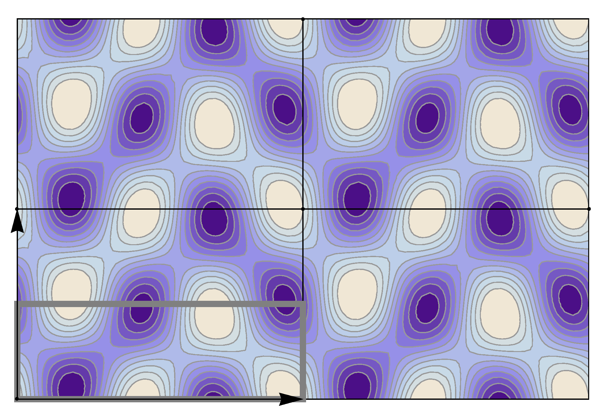
The power of establishing relation Equation (30) and the therefrom derived Fourier series Equations (32) and (33) is the reduction of the number of Fourier coefficients. The non-constant part can be characterised by 6 times less coefficients than for a “brute-force” approach without using the analytic result. In Figure 2 we show contours of an exemplary (real) function with hexagonal translation symmetry and 6-fold rotational symmetry with only two non-zero independent Fourier coefficients ( and ). The hexagonal translation and the 6-fold rotational symmetry are correctly observed.
3.2. Reflection Axes
A reflection about the axis (which can always be chosen parallel to the x-axis without loss of generality, see Table 1) is achieved by the coordinate transformation
Proceeding as for rotations, we put
This leads to the following system of Equations:
Continuing with the case of a hexagonal Bravais lattice, we obtain
and the property
Repeating the reflection results in the identity operation; this is consistent with property Equation (40) displaying a cycle of 2. Combining this symmetry operation with the 6-fold rotational symmetry of the preceding subsection results in the wallpaper group. The resulting restrictions on the Fourier coefficients are obtained by applying relation Equation (30) to both and , which leads to
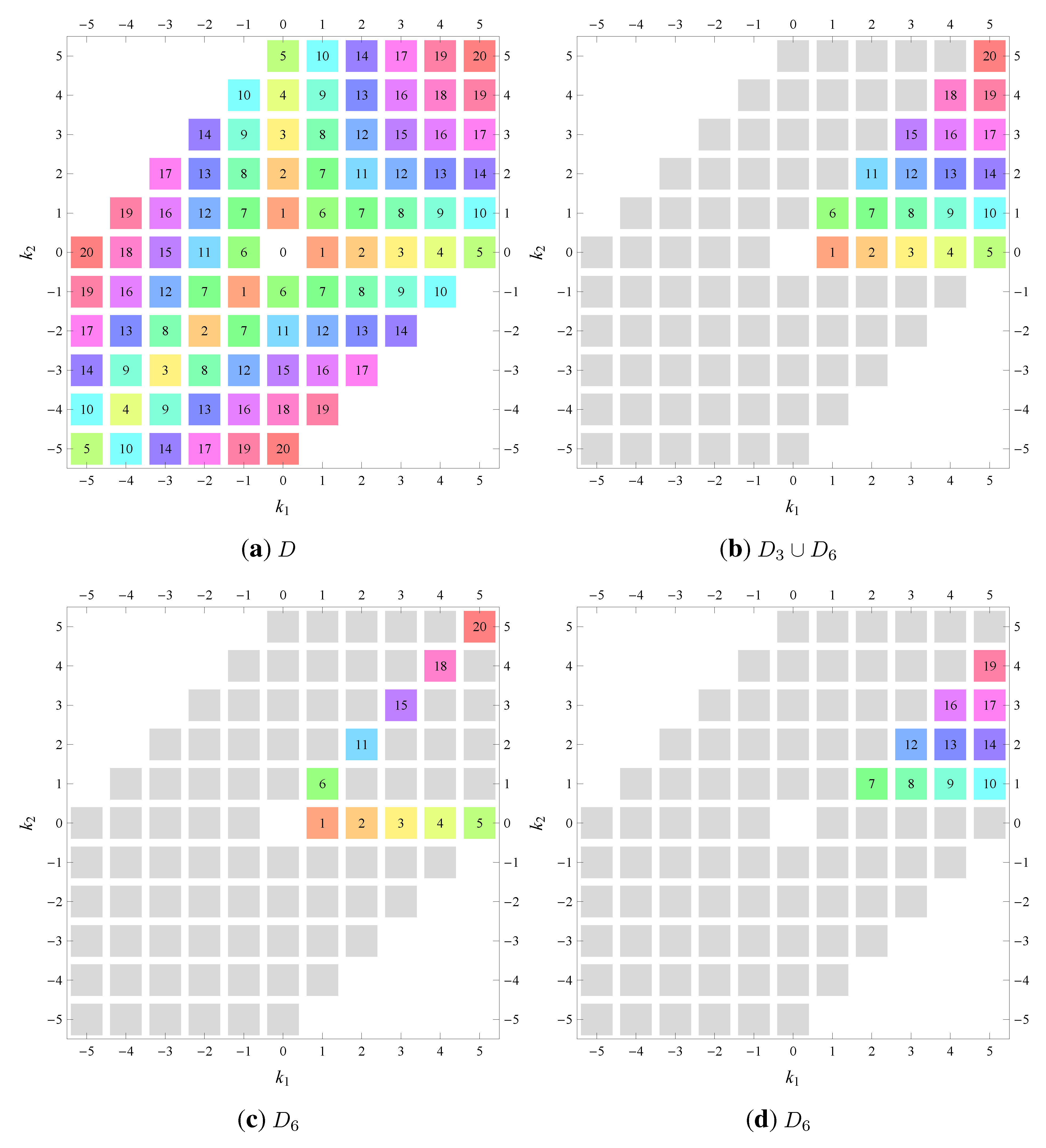
At first sight, we can then write a “reduced” Fourier series for as in Equation (32) with the indices running over a domain which now covers one-twelfth of the original space (excluding ). However, for some combinations of and , relation Equation (42) reduces to a 6-cycle. This can be seen in Figure 3(a) where we show the equivalence of points—according to relation Equation (42)—in a domain D. The points with for example all belong to sets of only 6 rather than 12 equivalent points. The domain containing representative ) points, shown in Figure 3(b), can be divided into a subdomain where points display a 6-cycle [Figure 3(c)] and a subdomain where points display a 12-cycle [Figure 3(d)]. The resulting Fourier series therefore needs to be formulated as
In a way, the coefficients in domain can be considered “doubly degenerate”. Note that technically, the point has a cycle of 1 (identity operation) and forms a domain by itself.
The criterion for points belonging to domain can be easily obtained by realizing that for , the cycle of 6 [Equation (30)] must “intersect” the cyle of 2 [Equation (40)]. We are therefore looking for solutions of the following 6 systems of Equations:
The respective solutions are:
These 6 relations correspond to 6 lines of points which are visually discernible in Figure 3(a).
The domain shown in Figure 3(b) is defined as the set of points for which and . For one has and ; is defined by and . The explicit Fourier expansion for a function with wallpaper group symmetry then reads:
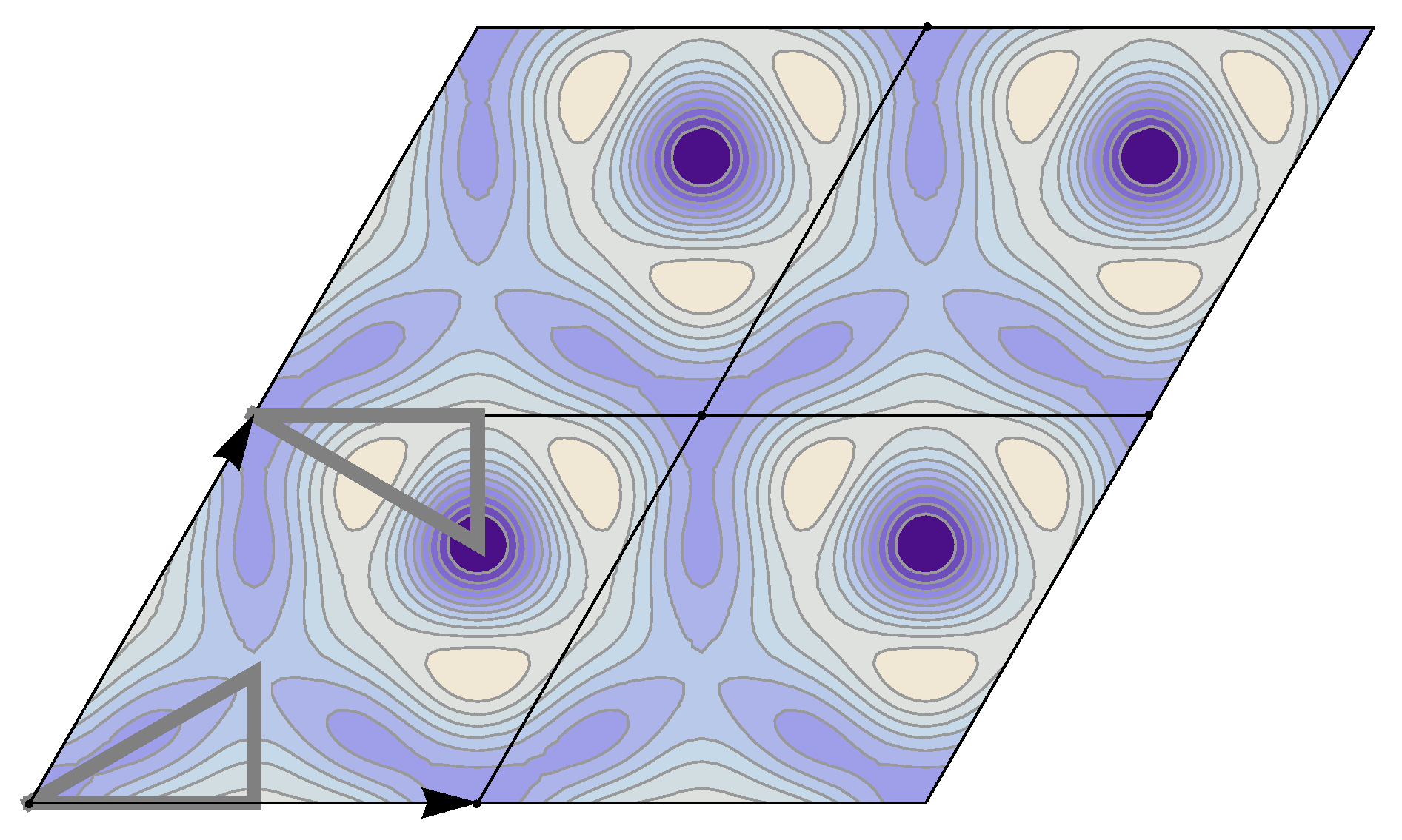
This rather complicated expression reflects the high symmetry of the group. (In fact, has the highest number of symmetry operations of all wallpaper groups.) Note that from this explicit expression, it follows that for to have no imaginary part, the coefficients need to be real—consistent with reality criterion Equation (8).
In Figure 4 we have plotted the contours of a real function with one independent non-zero Fourier coefficient from domain () and one non-zero coefficient from domain (). The honeycomb symmetry of the wallpaper group is nicely recovered.
We stress the importance of the foregoing symmetry analysis: A function displaying wallpaper group symmetry can be characterised with only a few independent Fourier coefficients. The wallpaper group is of particular interest because of the emergence of graphene [10] as a material with remarkable physical properties and promising applications.
3.3. Glide Reflection Axes
The last category of possible symmetry operations consists of glide reflection axes, combining a mirror operation about an axis with a translation parallel to that axis (the translation vector being half a lattice vector). Let us consider the glide reflection , with , transforming the point to according to
Imposing invariance of under the transformation implies
Because of the translational component of the symmetry operation , it is insufficient to propose a Fourier series for , equate the scalar products and , and solve as we did for rotational and mirror operations. Instead, we have to introduce a phase factor ,
and equate and for arbitrary . This leads to the following set of Equations:
As an example, let us take the wallpaper group , which has a rectangular lattice (reciprocal basis vectors and , see Table 1) and only a glide reflection axis () as a non-trivial symmetry operation. Equations (59)–(61) then reduce to
from which the following condition for the Fourier coefficients follows:
A function with wallpaper group symmetry can therefore be written as
As before, not all points display a cycle of 2 when repeatedly applying the transformation given by Equations (63) and (64). Points with form a domain with cycle 1; the remaining points () can be mapped onto a domain of representative points from which all coefficients can be calculated according to property Equation (65). In Equation (66) we have introduced the notation for the domain of points with cycle 1 excluding : . From Equation (65) it follows that for points in domain
which implies that for odd.
In Figure 5, we visualize the domains D, , and and the equivalence of Fourier coefficients. Equivalence through phase factors 1 and is marked by squares and discs, respectively. Necessarily vanishing Fourier coefficients [due to Equation (67)] are marked by the circle-in-square symbol “⌼”. It is again instructive to elaborate the Fourier expansion for into a more explicit form (displaying the rectangular lattice parameters a and b and using the ranges for domains and ). The result reads
Combining reality criterion Equation (8) with property Equation (65) results in the requirement ; this requirement indeed removes any imaginary part in expression Equation (69). It also establishes relations between coefficients within the domain . For example, , or from which it follows that must be real.
In Figure 6 we have plotted a real function with symmetry; the only non-vanishing independent Fourier coefficients are and . (The reality criterion then implies that and are then also non-zero.)
4. Derivation of Fourier Coefficient Relations
The foregoing examples show how to derive relations between the Fourier coefficients of a function with a given wallpaper group symmetry. In particular, we have discussed how to deal with a 6-fold rotation axis, a reflection axis, and a glide reflection axis. In this section, we will elaborate the symmetry properties of all other possible symmetry operations present in the wallpaper groups, and provide a summary. The restrictions on the Fourier coefficients for a specific wallpaper group then follow from combining symmetry properties (for example, the addition of a reflection axis to the group converts it into the group ). Our goal is to arrive at a table with an entry for each of the 17 wallpaper groups, containing all necessary information, in formulas and in a visualised form, concerning the Fourier expansion and the associated Fourier coefficients for the symmetry group.
4.1. Rotation Axes
Most wallpaper groups have a rotation axis at the origin of the unit cell. The transformation matrix for a 2-fold rotation at the origin reads
so that equating leads to
from which it follows that
The Fourier coefficients then obey the following 2-cycle:
In Table 2 we quote this symmetry property (together with the properties of the other symmetry operations). Note that this results does not depend on the lattice type, i.e., the lattice can be oblique, rectangular, centered rectangular, square, or hexagonal. The presence of a 2-fold symmetry axis with a square or hexagonal Bravais lattice implies a higher-order symmetry axis, however (4-fold and 6-fold, respectively). We therefore only quote the oblique, rectangular and centered rectangular lattices in the entry for ⬮ in Table 2.
For a 3-fold rotation, the rotation matrix reads
The existence of a 3-fold rotation axis implies a hexagonal lattice. With the hexagonal basis vectors given in Table 1, the equality of the scalar products and results in the following conditions:
The symmetry property for the Fourier coefficients then becomes
displaying—as it should—a 3-cycle.
The 4-fold rotation matrix reads
For a square lattice, required for a 4-fold rotation axis, the relation between and reads
which results in the following 4-cycle of Fourier coefficients:
Note that the requirement for a 2-fold symmetry axis is also fulfilled [Equation (73)].
The case of a 6-fold rotation axis (hexagonal Bravais lattice) has been treated in the previous section [Equation (30)]. It comprises both the 2-fold and 3-fold rotation axis conditions (and can in fact be constructed from combining these two).
4.2. Reflection Axes
The wallpaper groups are not distinguishable by rotation axes alone, as shown by the example of the and groups in the previous section. Other symmetry operations have to be considered. A first category is that of reflection axes. In the previous section we have treated the case when the x-axis is a reflection axis (which we from now on call reflection axis #1), for a hexagonal lattice. Here we consider the remaining possible lattices.
For a rectangular or a square lattice, Equations (36) and (37) lead to
so that
For a centered rectangular lattice, Equations (36) and (37) result in
Note that the combination of a rotation axis with a reflection axis can generate additional reflection axes. For example, in the case of the rectangular lattice with a 2-fold rotation axis, the x-axis being a reflection axis implies the y-axis also being a reflection axis. Only one of the two reflection axes is a generating (independent) symmetry element. The choice of which one of the two to include as a generating element is arbitrary, though. In Table 2, only (conveniently but otherwise arbitrarily chosen) generating elements are listed.
A second independent reflection axis (labelled #2) is present in the group (rectangular Bravais lattice). It is the line parallel to the x-axis and going through the point . The transformation law reads
In combination with a rectangular Bravais lattice, the phase factor and the relations read
The resulting Fourier symmetry property then reads
A third and final generating reflection axis (labelled #3) occurs in the group (hexagonal Bravais lattice). It is the line coinciding with the vector . The transformation has the same form as that of a rotation and reads
Equating and (no phase factor is required) gives
whence the symmetry property
4.3. Glide Reflection Axes
In SubSection 3.3 we considered the glide reflection axis encountered in the group (glide reflection axis #1 in Table 2). A second, independent, type of glide reflection axis (labelled #2) is found in the groups and : The line parallel to the x-axis going through the point is the axis, the shift vector is . The transformation reads
implying (for rectangular and square lattices)
so that
This completes our analysis of the Fourier symmetry properties resulting from symmetry operations encountered in the wallpaper groups; all results are summarized in Table 2.
4.4. Combining Rotation Axes and (Glide) Reflection Axes
With the help of Table 2, the symmetry properties for the Fourier coefficients can be derived for all wallpaper groups. The groups can be divided into two categories based on whether there is a rotation axis at the origin or not. The groups without a rotation axis are (the trivial group), , and ; their symmetry properties can be directly read out from Table 2. (For there are no restrictions on .) The groups exhibiting a rotation axis can be further subdivided into groups featuring additional symmetry elements and groups only containing the rotation axis. The latter are , , and ; their symmetry properties follow immediately from Table 2. The former groups are , , , , , , , and ; their Fourier coefficients obey conditions following from combining the rotation-axis property with the condition implied by the second (independent) symmetry element.
In SubSection 3.2 we showed how to combine a 6-fold rotational axis with reflection axis #1 resulting in the wallpaper group of graphene. To illustrate the procedure once more, we consider the wallpaper group . The presence of a three-fold rotation axis implies , while reflection axis #3 implies . Combining these two properties results in the identity of 6 Fourier coefficients:
For certain values of , this property breaks down to the identity of only 3 Fourier coefficients (3-cycle). The remaining combinations exhibit the full 6-cycle given by Equation (102). It is easy to show that the coefficients with a 3-cycle must obey one of the following 3 equations:
As before, the presence of cycles allows to take only independent Fourier coefficients from minimal domains (D and D, see Figure 7), and to write the general Fourier series for a function with symmetry as
Realising that domain contains the points for which and (see Figure 7) and that domain consists of the points with and , we arrive at the following explicit expression for :
Note that this equation connects points in domain . Indeed, taking with and results in , with . The reality criterion for therefore imposes further restrictions on the domain of independent Fourier coefficients. For example, the coefficient is equal to the complex conjugate of , and is equal to its own complex conjugate and hence real. In Figure 8, the function with and as only non-vanishing coefficients is shown.
4.5. Centering
When using the non-primitive basis for centered rectangular lattices, i.e., the rectangular basis , centering should be considered a symmetry operation of the unit cell and has to be accounted for appropriately.
To distinguish from the case where we use the non-primitive basis vectors (see Table 1), we write and for the Fourier summation indices and and for the Fourier coefficients. It is easy to show that the relations between and read
and
Clearly, the centering transformation law reads
A phase factor is required for matching Fourier series:
The result reads
so that the centering symmetry property becomes
from which it immediately follows that coefficients with odd have to vanish.
In Table 3 we list the Fourier coefficient properties for generating symmetry elements of the centered rectangular wallpaper groups in the non-primitive description. By combining the appropriate symmetry elements one obtains the Fourier properties for the Fourier coefficients :
Note that the and wallpaper groups are obtained by centering the and groups, respectively. On the level of Fourier expansions, the and Fourier series are simply obtained by taking the expressions for and , respectively, and excluding the terms for which is odd. The wallpaper group and its Fourier series can also be generated from centering the group.
4.6. Structure Factors in Crystallography
The implications of the foregoing mathematical considerations are widely used in crystallography and crystal structure determination. The periodic function one considers is the electronic density , the Fourier coefficients of which are known as the structure factors . The central formula expressing the space group (wallpaper group) symmetry reads [5,11]
with P and being the rotation and translation parts of the space group operations , respectively. Elaborating Equation (121) results in symmetry relations for the structure factors and is equivalent to carrying out the procedures described above for the various types of wallpaper group symmetry operations. In Vol. B of the “International Tables” [4,5,6,7,8], the functional forms of the Fourier expansions of the electronic density are tabulated in a compact way in structure-factor tables for wallpaper groups (Table A1.4.3.1 in [5]) and space groups (Tables A1.4.3.2–A1.4.3.7 in [5]). Note, however, that in the “International Tables” [4,5,6,7,8] the rather than the convention for hexagonal lattices (see Table 1) is used. In a (single-crystal) diffraction experiment, the symmetry relations between structure factors manifest themselves in the extinction and/or the equal (non-zero) intensity (proportional to ) of certain Bragg reflections. The Fourier coefficient maps, labeled “D”, shown throughout this paper and in Table 4, Table 5, Table 6, Table 7, Table 8, Table 9, Table 10, Table 11, Table 12, Table 13, Table 14, Table 15, Table 16, Table 17, Table 18, Table 19, Table 20, Table 21 and Table 22 (see below) are complementary to the information in the “International Tables” [4,5,6,7,8], and can be thought of as elementary diffraction patterns of functions (structures) with wallpaper group symmetry.
5. Wallpaper Group Tables
In the preceding sections we have shown how wallpaper group symmetry can be used to construct maximally-symmetric 2D Fourier series. The derivations and examples given contain many of the mathematical issues involved. At this point, it should be clear how to proceed for obtaining symmetry properties of Fourier coefficients and the Fourier series itself for a given wallpaper group.
We have made a systematical investigation of all wallpaper groups; in Table 4, Table 5, Table 6, Table 7, Table 8, Table 9, Table 10, Table 11, Table 12, Table 13, Table 14, Table 15, Table 16, Table 17, Table 18, Table 19, Table 20, Table 21 and Table 22 all relevant wallpaper group information (Fourier coefficients symmetry property, independent Fourier coefficients domains, Fourier series) is summarized visually and analytically. The upper part of each table contains the wallpaper group’s label, the Bravais lattice type, the direct and the reciprocal basis vectors. Then, an example (a contour plot spanning four unit cells of a real function ) displaying translational and point group symmetry is shown; the values of the non-vanishing Fourier coefficients used for the example are indicated below the contour plot. Basis vectors and a possible choice for the asymmetric unit are drawn on the figure. Next to the example, the domains showing equivalence of Fourier coefficients are shown. The total domain D shows which coefficients in the range are equivalent (equal or opposite); coordinates with equivalent Fourier coefficients are given a same color and number. When not all equivalent coordinates of a point lie in the range , that point is left blank and unnumbered. (This occurs only for the hexagonal wallpaper groups.) To the right of the total domain D, the subdomain containing exactly one independent representative (colored and numbered) of each set of equivalent points is shown; the remaining points are now shown shaded gray and unnumbered. For , an infinite number of possible choices exists; we recall that for a given cycle of Fourier coefficient indices generated by the symmetry property for Fourier coefficients, only one pair of indices should be contained within . For, e.g., (Table 5), one could equally well take , rather than , . Our choices for are simply based on convenience. In the case of subdomains with different cycles, the decomposition is shown below D and . The origin is always excluded from the subdomain (but included in the total domain D), which is why the notation is used for subdomains with cycle 1 excluding . Opposite Fourier coefficients are shown by discs and squares of the same color and labeled with a same number in the total domain D. In the case of necessarily vanishing Fourier coefficients, the symbol “⌼” is used. Below the example and the domains, the symmetry property for Fourier coefficients is given. To the right, if applicable, implications of the symmetry rule on the vanishing of Fourier coefficients (“extinction rules”) are given. Next, an explicit, symmetry-adapted, expression for the Fourier series of is given, containing only (apart from the term) independent coefficients from the subdomain . Finally, an elaborated version of the reality criterion is given: The complex conjugate of with is equated to an expression involving the same or another coefficient in . Implications on the reality of coefficients are given to the right, if applicable.
For the centered rectangular wallpaper groups and , alternate (non-primitive) versions of the tables are given as well, with Fourier indices labeled and (Table 9 and Table 14).
It is interesting to see how for each group, the real-space (point-group) symmetry is converted into coefficient-space symmetry. Indeed, the distribution of equivalent Fourier coefficients in domain D also displays rotation axes and mirror axes. Particularly intriguing is how the hexagonal groups divide coefficient space into 3-, 6- or 12-cycle domains.
6. Discussion and Conclusions
Having established Table 4, Table 5, Table 6, Table 7, Table 8, Table 9, Table 10, Table 11, Table 12, Table 13, Table 14, Table 15, Table 16, Table 17, Table 18, Table 19, Table 20, Table 21 and Table 22, it is useful to consider some points in more detail.
A first issue is the reality criterion. Trivially, for all wallpaper groups, for to be real, must be real. Considering general coefficients , it follows from Equation (8) and the symmetry property (Table 5) that for wallpaper groups having a 2-fold rotation axis at the origin, all coefficients must be real for to be real. Since in two dimensions a 2-fold rotation axis is equivalent to an inversion center, we can speak of centrosymmetric and non-centrosymmetric wallpaper groups. The reality criteria for the non-centrosymmetric groups are summarized in Table 23. As indicated already when discussing examples in the preceding sections, for a non-centrosymmetric wallpaper group, the reality criterion imposes further restrictions on the coefficients in the subdomain . In general, a coefficient in needs to be equal to the complex conjugate of another coefficient in ; in some special cases, this results in the reality of Fourier coefficients (see Table 23). It is important to note, however, that the definition in terms of matrices of the inversion operation used throughout the “International Tables” [4,5,6,7,8] is not only that the inversion matrix is the negative of the identity matrix but also that its determinant is negative. In that sense, there can be no inversion in two dimensions, and centrosymmetric and non-centrosymmetric wallpaper groups should rather be referred to as displaying and lacking 2-fold rotational symmetry, respectively.
A second point is the necessary vanishing of certain Fourier coefficients. As demonstrated in Section 2, a glide reflection axis introduces a phase factor in the symmetry property for the Fourier coefficients, which in turn leads to certain Fourier coefficients having to be zero. This occurs for the groups , , and (all containing a “g” in their label). Observed rules for vanishing coefficients are or , with . These are analogous to the diffraction extinction rules associated with the presence of glide reflection axes [4,5,6,7,8]. The centering operation discussed in SubSection 4.5 also implies Fourier coefficients to be zero (, )—in analogy with the diffraction extinction rules for centered unit cells [4,5,6,7,8].
A next issue is that of the notion of a “minimal” Fourier series. To correctly represent a given wallpaper group symmetry, a Fourier series must indeed contain sufficient non-vanishing Fourier coefficients resulting in the correct x- and y-dependence. Let us for example consider the group (Table 12). Trivially, if we take only the term we have no -dependence. If we take only or different from zero ( symmetry implies ) we create a function with only x- or y-dependence, respectively. This is illustrated in Figure 9(a,b). If we assign, however, simultaneously both to and non-zero values, we have a -dependent function, but its periodicity in both x- and y-direction is half that of the intended lattice, and the symmetry of the reduced unit cell is [Figure 9(c)]. The series with only “switched on” results in a function with the right translational symmetry, and does indeed have symmetry, but its asymmetric unit has half the size of the general asymmetric unit [Figure 9(d)]: The wallpaper group is actually (compare Table 12 and Table 14). While independence on x and/or y and periodicity reduction can be relatively easily avoided by inspecting the explicit expression of the Fourier expansion and including necessary (low- and low-) Fourier coefficients, the last observation (a Fourier series displaying symmetry) involves more subtle considerations. It can be understood by realising that the group is a subgroup of the group. A rectangular lattice Fourier series with (and all other Fourier coefficients equal to zero) fulfills both the symmetry properties of and , which can be clearly seen by comparing the domains D of Table 12 and Table 14. Even more, it also complies with the symmetry of the wallpaper group (Table 10), which is also a subgroup of (see also SubSection 4.5). The net symmetry will therefore be that of the higher-symmetry group, . To have a Fourier series with true (or ) symmetry, it is necessary to include non-zero coefficients with odd, as in the example in Table 12 where both and have been assigned non-zero values. Hence, to avoid apparent higher symmetry, a wallpaper group should be compared with any supergroup of which it is a subgroup; its pattern of non-zero and equivalent Fourier coefficients should distinguish itself from that of the supergroup. As a further illustration, let us consider the wallpaper groups and (Table 21 and Table 22, respectively). The former is a subgroup of the latter. If the expression for the Fourier expansion for a function contains only Fourier coefficients that belong to the subdomain of the group, this will result in a function displaying symmetry. A true function therefore needs to contain at least one non-zero Fourier coefficient from the - subdomain. The example functions in the preceding sections and in Table 4, Table 5, Table 6, Table 7, Table 8, Table 9, Table 10, Table 11, Table 12, Table 13, Table 14, Table 15, Table 16, Table 17, Table 18, Table 19, Table 20, Table 21 and Table 22 have been selected carefully to yield true wallpaper group symmetry with a small number of non-vanishing Fourier coefficients (in every example, only two independent coefficients were assigned non-zero values).
A more formal approach for deriving minimal symmetry-adapted functions for the wallpaper groups involves group theory; each wallpaper group should be decomposed into irreducible representations (IRREPs) [12]. The terms of the Fourier series developed in this work should then be rearranged into linear combinations that belong to the different IRREPs of the wallpaper group. The linear combinations belonging to the unit representation then display the full wallpaper group symmetry without apparent higher symmetry [13]. The situation is similar to the decomposition of (planar) point groups. For example, the lowest-order function displaying point group symmetry is or, in polar coordinates, . A decomposition of the wallpaper groups into IRREPs is beyond the scope of the present paper.
Finally, a few suggestions on how to use the Fourier series developed in this work. Our motivation came from the need of a continuous and infinitely differentiable function with the symmetry of the graphene lattice—i.e., the wallpaper group. In the context of solid-state physics, the 2D functions with wallpaper group symmetry that naturally come to mind are (complex) electronic wave functions or (real) electronic densities of the new family of 2D materials like graphene or boron-nitride. Electronic densities can nowadays be calculated from ab-initio principles; a first application of our calculations could therefore be the fit of an ab-intio obtained electronic density to the symmetry-adapted Fourier series. By limiting the number of fitted coefficients [calculated numerically via Equation (6)], one obtains a handy, analytical expression for , which can then subsequently be used in further calculations. If necessary, the extension of the density above and below the atomic plane can be taken into account by making the Fourier coefficients z-dependent.
Another situation where symmetry-adapted Fourier series could be used is when fitting X-ray diffraction data to a structural model. Rather than putting atoms in the unit cell and adjusting their positions and the unit cell’s parameters, one could conceive an approach where a limited number of Fourier coefficients of the electronic density —responsible for the scattering of X-rays—is taken as the adjustable parameter set (together with the unit cell’s dimensions), after which an atomic distribution matching the electronic density can be sought.
Note that the results obtained here can also be used for identifying or discriminating wallpaper groups (see e.g., [14]): A numerical calculation of the Fourier coefficients of a given function and testing for Fourier coefficient symmetry properties can indeed help to distinguish the planar symmetry of .
Planar wallpaper groups are not only relevant for describing 2D crystals but also useful for analysing surfaces of three-dimensionally periodic crystals, and they can be a tool for studying crystal growth [15].
In summary, it is hoped that the symmetry-adapted Fourier series presented in this paper will turn out to be useful for dealing with periodic functions in two dimensions in various situations.
Acknowledgments
Useful discussions with N.V. Tarakina are gratefully acknowledged. The author is a Research Fellow of the Research Foundation-Flanders (F.W.O.—Vlaanderen).
References
- Fedorov, E.S. Nachala Ucheniia O Figurakh (in Russian). Zap. Min. Obshch. 1885, 21, 240–516. [Google Scholar]
- Fedorov, E.S. Simmetriia Pravil’nykh Sistem Figur (in Russian). Zap. Min. Obshch. 1891, 28, 1–146. [Google Scholar]
- Fedorov, E.S. Zametka Ob Uspekhakh Teoreticheskoi Kristallografii Za Poslednee Desiatiletie (in Russian). Zap. Min. Obshch. 1890, 26, 374–375. [Google Scholar]
- Hahn, T. International Tables for Crystallography, Volume A; The International Union of Crystallography: Chester, UK, 2005. [Google Scholar]
- Shmueli, U. International Tables for Crystallography, Volume B; The International Union of Crystallography: Chester, UK, 2001. [Google Scholar]
- Prince, E. International Tables for Crystallography, Volume C; The International Union of Crystallography: Chester, UK, 2004. [Google Scholar]
- Authier, A. International Tables for Crystallography, Volume D; The International Union of Crystallography: Chester, UK, 2003. [Google Scholar]
- Kopský, V.; Litvin, B. International Tables for Crystallography, Volume E; The International Union of Crystallography: Chester, UK, 2002. [Google Scholar]
- Kittel, C. Energy bands. Introduction to Solid State Physics, 7th ed.; John Wiley Sons Inc.: New York, NY, USA, 1996; Chapter 7. [Google Scholar]
- Geim, A.K.; Novoselov, K.S. The rise of graphene. Nat. Mater. 2007, 6, 183–191. [Google Scholar] [CrossRef] [PubMed]
- Waser, J. Symmetry relations between structure factors. Acta Cryst. 1955, 8, 595. [Google Scholar] [CrossRef]
- Tinkham, M. Group Theory and Quantum Mechanics; McGraw-Hill: New York, NY, USA, 1964. [Google Scholar]
- Bradley, C.J.; Cracknell, A.P. The Mathematical Theory of Symmetry in Solids. Clarendon: Oxford, UK, 1972. [Google Scholar]
- Landwehr, K. Visual discrimination of the 17 plane symmetry groups. Symmetry 2011, 3, 207–219. [Google Scholar] [CrossRef]
- Grundmann, M. Formation of epitaxial domains: Unified theory and survey of experimental results. Phys. Status Solidi B 2011, 248, 805–824. [Google Scholar] [CrossRef]
Figure 1.
wallpaper group. (a) Map of points in domain D. Equivalent points, having equal Fourier coefficients , are assigned a same color and number. The points in the top left and bottom right white zones have equivalent points falling outside the range and are therefore not included in D. Note the “distorted” hexagonal symmetry; (b) Domain containing one representative point of each set .

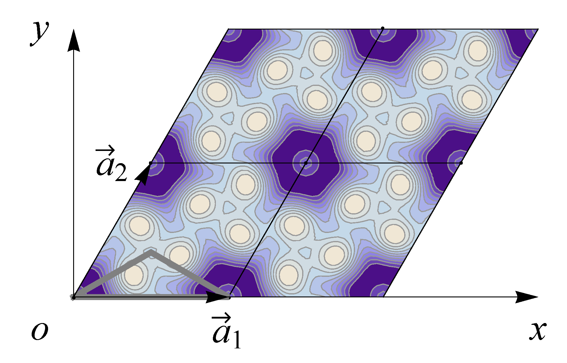
Figure 2.
Real function ) with symmetry; the only non-zero Fourier coefficients are and . Basis vectors of the unit cell as well as the asymmetric unit (bound by gray lines) are shown.
Figure 2.
Real function ) with symmetry; the only non-zero Fourier coefficients are and . Basis vectors of the unit cell as well as the asymmetric unit (bound by gray lines) are shown.

Figure 3.
wallpaper group. (a) Map of points in domain D; equivalent points are shown with a same color and number. Note the higher symmetry (less representative points) than for the wallpaper group [see Figure 2(a)]; (b) Domain containing representative points; (c) Domain containing representative points with a cycle of 6; (d) Domain containing representative points with a cycle of 12.

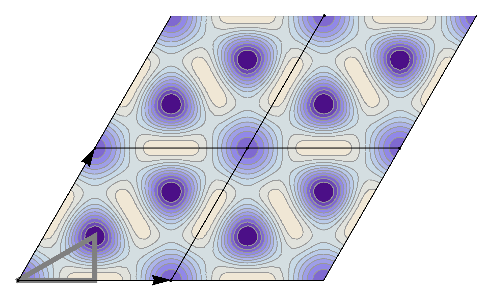
Figure 4.
Real function ) with symmetry; the only non-zero Fourier coefficients are and . Basis vectors of the unit cell as well as the asymmetric unit (bound by gray lines) are shown.
Figure 4.
Real function ) with symmetry; the only non-zero Fourier coefficients are and . Basis vectors of the unit cell as well as the asymmetric unit (bound by gray lines) are shown.

Figure 5.
wallpaper group. (a) Map of points in domain D. Equivalent points are shown with a same color and number; (b) Domain containing representative points; (c) Domain containing representative points with a cycle of 1, excluding ; (d) Domain containing representative points with a cycle of 2. The equivalence relation [Equation (65)] involves a phase factor ; points outside the representative domain for which and are marked by squares and discs, respectively. Vanishing Fourier coefficients are marked by the symbol “⌼”.

Figure 6.
Real function ) with symmetry; the only non-zero independent Fourier coefficients are and . Basis vectors of the unit cell as well as the asymmetric unit (bound by gray lines) are shown.
Figure 6.
Real function ) with symmetry; the only non-zero independent Fourier coefficients are and . Basis vectors of the unit cell as well as the asymmetric unit (bound by gray lines) are shown.

Figure 7.
wallpaper group. (a) Map of points in domain D; equivalent points are shown with a same color and number; (b) Domain containing representative points; (c) Domain containing representative points with a cycle of 3; (d) Domain containing representative points with a cycle of 6.
Figure 7.
wallpaper group. (a) Map of points in domain D; equivalent points are shown with a same color and number; (b) Domain containing representative points; (c) Domain containing representative points with a cycle of 3; (d) Domain containing representative points with a cycle of 6.

Figure 8.
Real function ) with symmetry; the only non-zero Fourier coefficients are and [implying , see Equation (108)]. Basis vectors of the unit cell as well as the asymmetric unit (bound by gray lines) are shown.
Figure 8.
Real function ) with symmetry; the only non-zero Fourier coefficients are and [implying , see Equation (108)]. Basis vectors of the unit cell as well as the asymmetric unit (bound by gray lines) are shown.

Figure 9.
Incomplete realisations of the wallpaper group: (a) ; (b) ; (c) ; (d) . The general asymmetric unit is shown with dashed lines, the actual asymmetric unit with full lines.
Figure 9.
Incomplete realisations of the wallpaper group: (a) ; (b) ; (c) ; (d) . The general asymmetric unit is shown with dashed lines, the actual asymmetric unit with full lines.


Table 1.
Basis vectors and reciprocal basis vectors of the 5 planar Bravais lattices. For the non-centered lattices, can always be chosen parallel to without loss of generality. For the hexagonal lattice, the angle between the basis vectors is taken to be rather than .
Table 1.
Basis vectors and reciprocal basis vectors of the 5 planar Bravais lattices. For the non-centered lattices, can always be chosen parallel to without loss of generality. For the hexagonal lattice, the angle between the basis vectors is taken to be rather than .
| oblique | ||
| rectangular | ||
| centered rectangular | ||
| square | ||
| hexagonal | ||
Table 2.
Fourier coefficient properties for generating symmetry elements of the 16 non-trivial wallpaper groups.
Table 2.
Fourier coefficient properties for generating symmetry elements of the 16 non-trivial wallpaper groups.
| symmetry operation | Bravais lattice | Fourier coefficients | wallpaper groups |
|---|---|---|---|
| ⬮ | oblique | ||
| rectangular | , , | ||
| centered rectangular | |||
| ▲ | hexagonal | , , | |
| ◆ | square | , , | |
| ⬢ | hexagonal | , | |
| reflection axis #1 | rectangular | , | |
| square | |||
| centered rectangular | , | ||
| hexagonal | , | ||
| glide reflection axis #1 | rectangular | ||
| reflection axis #2 | rectangular | ||
| glide reflection axis #2 | rectangular | ||
| square | |||
| reflection axis #3 | hexagonal |
Table 3.
Fourier coefficient properties for generating symmetry elements of the centered rectangular wallpaper groups.
Table 3.
Fourier coefficient properties for generating symmetry elements of the centered rectangular wallpaper groups.
| symmetry operation | Bravais lattice | Fourier coefficients | wallpaper groups |
|---|---|---|---|
| centering | centered rectangular | , | |
| ⬮ | centered rectangular | ||
| reflection axis #1 | centered rectangular | , |
Table 4.
oblique | ||
 |  |  |
Table 5.
oblique | ||
 |  |  |
Table 6.
rectangular | ||
 |  |  |
 |  | |
Table 7.
rectangular | ||
 |  |  |
 |  | |
Table 8.
centered rectangular | ||
 |  |  |
 |  | |
Table 9.
—non-primitive basis.
rectangular | ||
 |  |  |
 |  | |
Table 10.
rectangular | ||
 |  |  |
 |  | |
Table 11.
rectangular | ||
 |  |  |
 |  | |
Table 12.
rectangular | ||
 |  |  |
 |  | |
Table 13.
centered rectangular | ||
 |  |  |
 |  | |
| () | ||
Table 14.
—non-primitive basis.
rectangular | ||
 |  |  |
 |  | |
Table 15.
.
square | ||
 |  |  |
Table 16.
square | ||
 |  |  |
 |  | |
Table 17.
square | ||
 |  |  |
 |  | |
Table 18.
hexagonal | ||
 |  |  |
Table 19.
hexagonal | ||
 |  |  |
 |  | |
Table 20.
hexagonal | ||
 |  |  |
 |  | |
Table 21.
hexagonal | ||
 |  |  |
Table 22.
hexagonal | ||
 |  |  |
 |  | |
Table 23.
Non-centrosymmetric wallpaper groups and their reality criteria.
| Bravais lattice | wallpaper group | reality criterion | |
|---|---|---|---|
| general | special | ||
| oblique | |||
| rectangular | |||
| centered rectangular | |||
| hexagonal | |||
© 2012 by the author; licensee MDPI, Basel, Switzerland. This article is an open access article distributed under the terms and conditions of the Creative Commons Attribution license (http://creativecommons.org/licenses/by/3.0/).
Share and Cite
MDPI and ACS Style
Verberck, B. Symmetry-Adapted Fourier Series for the Wallpaper Groups. Symmetry 2012, 4, 379-426. https://doi.org/10.3390/sym4030379
AMA Style
Verberck B. Symmetry-Adapted Fourier Series for the Wallpaper Groups. Symmetry. 2012; 4(3):379-426. https://doi.org/10.3390/sym4030379
Chicago/Turabian StyleVerberck, Bart. 2012. "Symmetry-Adapted Fourier Series for the Wallpaper Groups" Symmetry 4, no. 3: 379-426. https://doi.org/10.3390/sym4030379