The Symmetric-Partitioning and Incremental-Relearning Classification and Back-Propagation-Network Tree Approach for Cycle Time Estimation in Wafer Fabrication

Abstract
: An innovative classification and back-propagation-network tree (CABPN tree) approach is proposed in this study to estimate the cycle time of a job in a wafer fabrication factory, which is one of the most important tasks in controlling the wafer fabrication factory. The CABPN tree approach is an extension from the traditional classification and regression tree (CART) approach. In CART, the cycle times of jobs of the same branch are estimated with the same value, which is far from accurate. To tackle this problem, the CABPN tree approach replaces the constant estimate with variant estimates. To this end, the cycle times of jobs of the same branch are estimated with a BPN, and may be different. In this way, the estimation accuracy can be improved. In addition, to determine the optimal location of the splitting point on a node, the symmetric partition with incremental re-learning (SP-IR) algorithm is proposed and illustrated with an example. The applicability of the CABPN tree approach is shown with a real case. The experimental results supported its effectiveness over several existing methods.1. Introduction
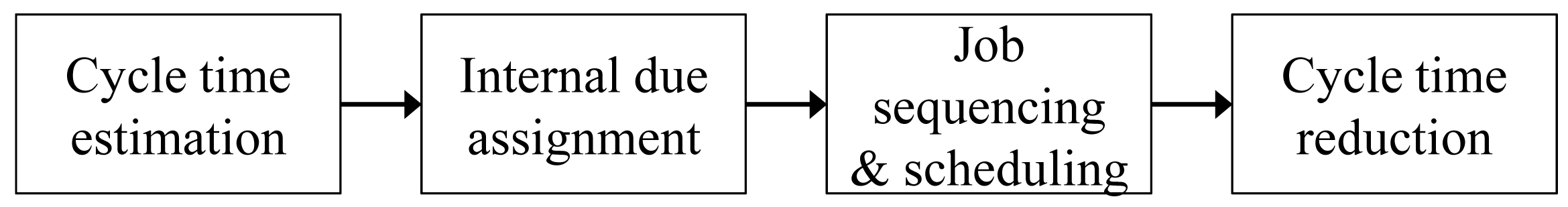
The cycle time (flow time, manufacturing lead time) of a job is the time required for the job to go through the factory. Therefore, it is subject to capacity constraints, the factory congestion level, the quality of job scheduling, and many other factors. As a result, the cycle time of a job is highly uncertain. Cycle time management activities include cycle time estimation, internal due date assignment, job sequencing and scheduling, and cycle time reduction (see Figure 1). In practice, shortening the cycle times of jobs is considered an effective way to improve the responsiveness to changes in demand [1]. In addition, according to [2], the number of defects per die has a positive relationship with the cycle time, which means shortening the cycle time can improve product quality. Further, estimating the cycle time of a job helps establish the internal due date for the job.
In the literature, various types of methods have been proposed to estimate the cycle time of a job in a factory. For example, probability-based statistical methods, such as queuing theory and regression, have been proposed. In [3], Kingman's formula that considers utilization, the coefficient of variation of arrival times, and the mean service time was proposed to analyze the cycle time of a job. However, that can only be applied to a single process step, and may be ineffective when applied to a whole production line [1]. Furthermore, in these studies, some restrictive assumptions were made, such as exponential processing time distribution [4]. Recently, Pearn et al. [5] fitted the waiting time of a job in a wafer fabrication factory with a Gamma distribution. After adding the waiting time to the release time, the cycle time can be derived, which is one of the most important tasks in controlling a wafer fabrication factory. However, the fitted distribution quickly became invalid, making some cycle time estimates far from accurate [6]. Chen [7] fitted a fuzzy linear regression (FLR) equation to estimate the cycle time of a job in a wafer fabrication factory. A precise range of the cycle time was also determined. To the same purposes, Chien et al. [8] fitted a nonlinear regression equation instead. Chen [6] applied classification and regression tree (CART) to estimate the cycle time of each job in a wafer fabrication factory. Principal component analysis (PCA) was also applied to generate independent variables from the original ones, which then served as the new inputs to CART.
The application of artificial neural networks (ANNs) is also a mainstream in this field. For example, a self-organization map (SOM) was developed in Chen [9] to classify the jobs in a wafer fabrication factory into a number of categories. Chen [10] and Chang and Hsieh [11] have constructed back propagation networks (BPNs) (or feed-forward neural networks, FNNs) to estimate the cycle time of a job based on the attributes of the job and the current factory conditions. These studies indicated that linear methods are incapable of estimating the cycle time of a job, which supported the application of nonlinear methods such as ANNs. In addition, to improve the effectiveness of an ANN approach, classifying jobs before (or after) estimating the cycle times have been shown to be a viable strategy. To this end, several classifiers were applied, such as k-means (kM) [12], fuzzy c-means (FCM) [13], and SOM [9,14]. A common feature of these classifiers is that all attributes of a job are considered at the same time. In contrast, there are classifiers that consider only some of the job attributes, such as CART. The joint use of CART and BPN for estimating the cycle time of a job has rarely been discussed in this field.
An innovative classification and back-propagation-network tree (CABPN tree) approach is proposed in this study to estimate the cycle time of a job in a wafer fabrication factory. The CABPN tree approach is an extension from the traditional classification and regression tree (CART) approach. The significance of doing so is fourfold:
- (1)
In CART, the cycle times of jobs of a branch are estimated with the same value, which is not accurate. In the proposed CABPN tree approach, a BPN is constructed for each branch to estimate the cycle times of jobs, which is expected to enhance the estimation accuracy;
- (2)
Although clusterwise models such as SUPPORT and treed Gaussian process models have been used in various fields, they have not been applied to estimating the cycle time of a job in a manufacturing system;
- (3)
Compared with the existing methods, the proposed CABPN tree approach classifies jobs based on fewer job attributes. On one hand, it is easier to implement. On the other hand, it is possible to assign more jobs to a branch;
- (4)
The existing classifiers in this field, such as kM, FCM, and SOM, classify jobs based on their attributes rather than their compatibilities with the estimation mechanism. However, the compatibility with the estimation mechanism is important, and may be more influential to the estimation performance. In this regard, CART considers the estimation performance in classifying jobs, which makes it more suitable for the same purpose.
In addition, to determine the optimal location of the splitting point on a node, the symmetric partition with incremental re-learning (SP-IR) algorithm is proposed. The proposed CABPN tree approach is a hybrid approach that fulfills both the classification and regression tasks. Table 1 is used to compare the proposed CABPN tree approach with some existing methods.
The proposed CABPN tree approach is introduced in Section 2. In addition, the SP-IR algorithm is illustrated with a small example. Subsequently, in Section 3, a real case containing the data from a wafer fabrication factory was used to evaluate the effectiveness of the proposed methodology. Several existing methods in this field have been applied to the same case to make a comparison. The advantages and/or disadvantages of each method were discussed. Finally, Section 4 concludes this paper and puts forward some directions that can be explored in future studies.
2. Methodology
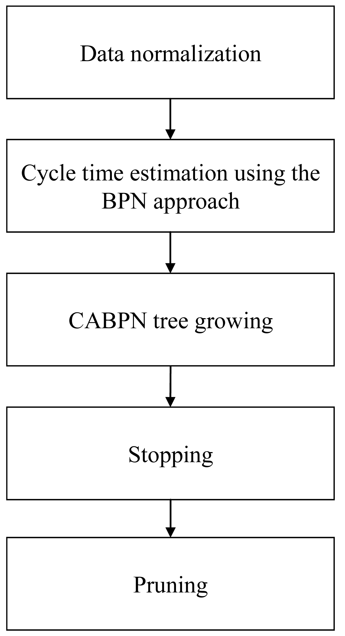
There are five steps in the proposed methodology: data normalization, cycle time estimation using the BPN approach, CABPN tree growing, stopping, and pruning, as illustrated in Figure 2.
In the traditional CART approach, the cycle times of jobs assigned to a branch (b) are estimated with the same value y(b) that is equal to the average of the historical cycle times:
2.1. Normalization
First, the collected data are normalized into [0.1, 0.9]:
Lemma 1
The normalized value can be converted back to
Conversely, the ranges of the inputs and output of the BPN are set to [0, 1]. In this way, the future value may be greater than the historical maximum or less than the historical minimum [9].
Theorem 1
Assume max x/min x = ξ. The future value of x, say xf, may be greater than max x by (12.5 − 12.5/ξ)% or less than min x by (12.5ξ – 12.5)%.
Proof
The historical values of x are normalized into [0.1, 0.9]. However, the BPN accepts an input between 0 and 1. For this reason, the normalized value of a future value xf according to the historical maximum and minimum, N(xf), may be up to 1,
It is also acceptable to normalize an input into a narrower range, such as [0.2, 0.8] or [0.3, 0.7], to allow for a larger or smaller future value. However, the fluctuation in the input will be further smoothened in this way; that is not beneficial to fit an exact relationship between the input and the output.
2.2. Estimating the Cycle Times of Jobs Using a BPN
Subsequently, a BPN is constructed to estimate the cycle times of jobs. The BPN is configured as follows. There are K inputs to the BPN including the attributes of a job and the factory conditions when the job was released into the factory. A lot of past studies have shown that a BPN with a single hidden layer can achieve a satisfactory approximation performance [12–17]. In addition, several ways have been proposed in the literature to determine the number of neurons in the hidden layer, e.g., [18,19]. A common practice is to set it to the double of the number of inputs [9,17], i.e., 2K. The activation/transformation functions for the input and hidden layers are the linear activation function and the hyperbolic tangent sigmoid function, respectively:
Inputs to the BPN are multiplied by the weights of the connections between the input and hidden layers, then are summed on each neuron in the hidden layer. After being compared with the threshold on the neuron, only significant signals will be transformed and outputted as:
Signals outputted from the hidden-layer neurons are transmitted to the neuron in the output layer in the same manner. Finally, the output from the BPN is generated as:
Subsequently, a lot of algorithms can be applied to train a BPN, such as the gradient descent (GD) algorithm, the conjugate gradient algorithm, the Levenberg-Marquardt (LM) algorithm, the Broyden-Fletcher-Goldfarb-Shanno (BFGS) algorithm, and others. For a recent comparison of these algorithms, refer to [17]. Among these algorithms, the LM algorithm has a faster convergence speed, and therefore is applied in the proposed methodology, as described below.
First, placing the inputs and the BPN parameters in vectors
- (1)
Specify the initial values of β, e.g., β = [1, 1, …, 1].
- (2)
Replace β by β + δ, where :
- (3)
Approximating the right-hand side by its linearization gives
where,is the gradient vector of f with respect to β. SSE becomes- (4)
The optimal value of δ can be obtained by taking the derivative of SSE with respect to δ and setting the result to zero.
- (5)
Return to Step (2).
Artificial neural networks such as BPN, radial basis function (RBF) network, and support vector regression (SVR) are effective methods to carry out nonlinear approximation. However, the dynamic environment in a wafer fabrication factory is quite complex. A number of studies (e.g., [11,12]) have shown that the relationship between the attributes and cycle time of a job in such an environment cannot be described with a single function. Therefore, jobs have to be classified before estimating the cycle times. Direct applications of BPN, RBF, or SVR are not very effective.
2.3. BPN Tree Growing
This step is to grow the CABPN tree using a recursive partitioning technique that selects variables and split points according to a pre-specified criterion. In the traditional CART approach, such criteria include Gini, towing, ordered towing, and maximum deviance reduction [15,16].
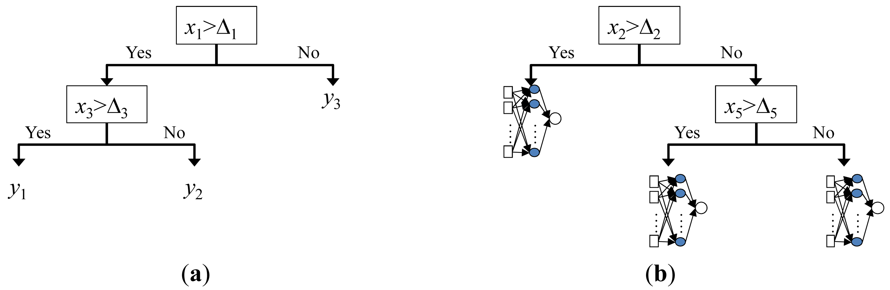
In the beginning, all jobs are assigned to the current node. Assume jobs of the current node are put in a set G = {j(p) | p = 1 ∼ q}. Sorting the data of these jobs along attribute k gives another set , k = 1 ∼ K. Splitting Gk at the point between and gives two subsets and , i.e., the splitting point is between jobs r and r + 1. Two BPNs, indicated with BPN1(x,β1) and BPN2(x,β2), are constructed to estimate the cycle times of jobs in the two subsets, respectively. An optimal split on the current node is the one that minimizes the impurity measure Imp(k,r):
To help solve this problem, the symmetric partition with incremental re-learning (SP-IR) algorithm is proposed as follows:
Step 1: Set k = 1;
Step 2: Sort the jobs along attribute k;
Step 3: Partition Gk into two equal subsets, i.e., r = q/2;
Step 4: Construct and train two BPNs to estimate the cycle times of jobs in the two subsets;
Step 5: Calculate the impurity measure Imp(k,r);
Step 6: Move the splitting point one job forward. Re-train BPN1 by adding the data of the new job;
Step 7: Re-calculate Imp(k,r). If it is improved, return to Step 6; otherwise, go to Step 8;
Step 8: Move the splitting point one job backward. Re-train BPN2 by adding the data of the new job;
Step 9: Re-calculate Imp(k,r). If it is improved, return to Step 8; otherwise, go to Step 9;
Step 10: Compare the results of Steps 7 and 9. The better result determines the optimal location of the splitting point along attribute k;
Step 11: k = k + 1;
Step 12: If k = K, stop; otherwise, return to Step 2.
The retraining process uses the parametric values at the end of the previous training as the initial setting, and train the BPN with fewer epochs. In this way, it is likely that the new optimal solution will be close to that in the previous training.
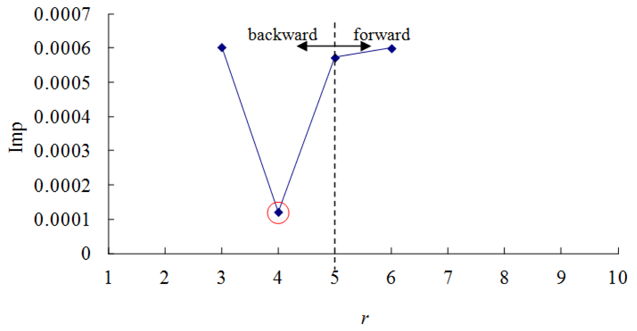
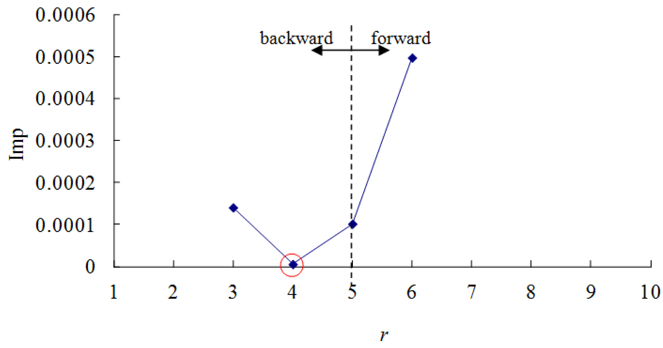
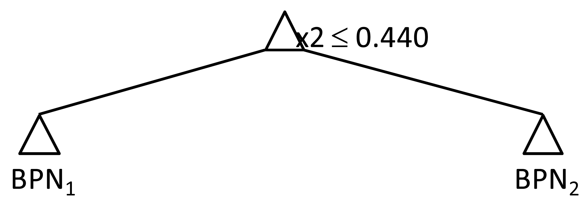
An example is provided in Table 3 to illustrate the SP-IR algorithm. At first, set k to 1, so G1 = {j1, j2, j7, j5, j6, j4, j3, j10, j8, j9}. Set r to 5, so and . Two BPNs, BPN1 and BPN2, were constructed to estimate the cycle times of jobs in the two subsets, respectively. The impurity measure Imp(k,r) was calculated as 5.06 × 10⁻⁴. The improvement in Imp(k,r) by moving the splitting point was summarized in Figure 4. Obviously, the optimal splitting point was r = 4, i.e., one job backward. In this way, jobs were partitioned into two subsets {j1, j2, j7, j5} (xj1 ≤ 0.304) and {j6, j4, j3, j10, j8, j9} (xj1 > 0.304). The minimum impurity was 1.21 × 10⁻⁴. Subsequently, the data were partitioned along the second attribute in the same way, and the results were summarized in Figure 5. The jobs were partitioned into {j5, j10, j1, j3} (xj2 ≤ 0.440) and {j6, j9, j2, j7, j8, j4} (xj2 > 0.440). The minimum impurity was 6.04 × 10⁻⁶. After comparing the two results, the better way for the current node is to partition the jobs along the second attribute, because the impurity can be reduced to a smaller value (see Figure 6).
2.4. Stopping
The growing of a CABPN tree stops if any of the following conditions has been satisfied:
- (1)
The improvement in the performance measure, i.e., the impurity measure, has become insignificant with more branches;
- (2)
A certain number of nodes have been generated;
- (3)
The depth of the tree has reached a certain level.
2.5. Pruning
A large CABPN tree may overfit, while a small CABPN tree may not reflect the inherent structure of the data. Cost-complexity pruning is usually used to tackle this issue. The cost-complexity of a CABPN tree T is the sum of SSE and the penalty on the complexity/size of the tree:
The results of cost-complexity pruning are a nested subset of CABPN trees starting from the largest tree and ending with the smallest tree (i.e., a tree with only a single node). The effectiveness of a subtree can be evaluated by cross-validation or using another (testing) data.
3. Applications
A real case containing the data of 200 jobs from a dynamic random access memory (DRAM) manufacturing factory was used to evaluate the effectiveness of the proposed methodology (see Table 4). The factory is located in Taichung Scientific Park of Taiwan, and has a monthly capacity of about 20,000 pieces of wafers. Jobs in a batch of about 25 wafers are released into the factory in a relatively stable pattern. The prioritized first-come first-serve (p-FCFS) policy is used to sequence jobs on each machine, i.e., jobs are first sequenced according to their priorities, then by their arrival times at the machine. The relationship between the cycle times and five attributes of jobs were fitted to estimate the cycle time of a new job. The backward elimination of regression analysis is applied to screen potential variables, for which the adjusted coefficient of determination (the adjusted R2) is used to evaluate the effectiveness of deleting a variable. Finally, four attributes are chosen: xj1 (the job size), xj2 (the queue length before the bottleneck), xj3 (the average waiting time of jobs already finished), and xj4 (factory utilization). Jobs in the collected data were of the same product type and priority. The average and standard deviation of the cycle times were 1225 and 206 h. Obviously, there was a considerable fluctuation in the cycle times. The data of the first 150 jobs were used as the training examples, while the remaining data were reserved for testing.
The collected data were normalized into [0.1, 0.9], as shown in Table 5. This step is not required in the traditional CART method. Subsequently, a CABPN tree was to be built for the normalized data. For each category, a BPN was constructed to estimate the cycle times of jobs. BPN was implemented using the Neural Network Toolbox of MATLAB 2006a with the following topology:
- (1)
A single hidden layer with eight nodes;
- (2)
Number of epochs per replication: 1000;
- (3)
Training algorithm: the LM algorithm;
- (4)
Stop training if the mean squared error (MSE) < 10−4 or 1000 epochs have been run;
- (5)
Early stopping: After each epoch of training, the BPN is applied to the testing data. If the performance, measured in terms of MSE, begins to deteriorate, the training process stops to avoid overfitting.
The CABPN tree was grown using the proposed SP-IR algorithm. The criteria for stopping the CABPN tree growing include:
- (1)
The improvement in the SSE was less than 5%;
- (2)
More than 10 nodes have been generated;
- (3)
The depth of the CABPN tree has reached the third level.
These stopping criteria are also beneficial to avoid overfitting.
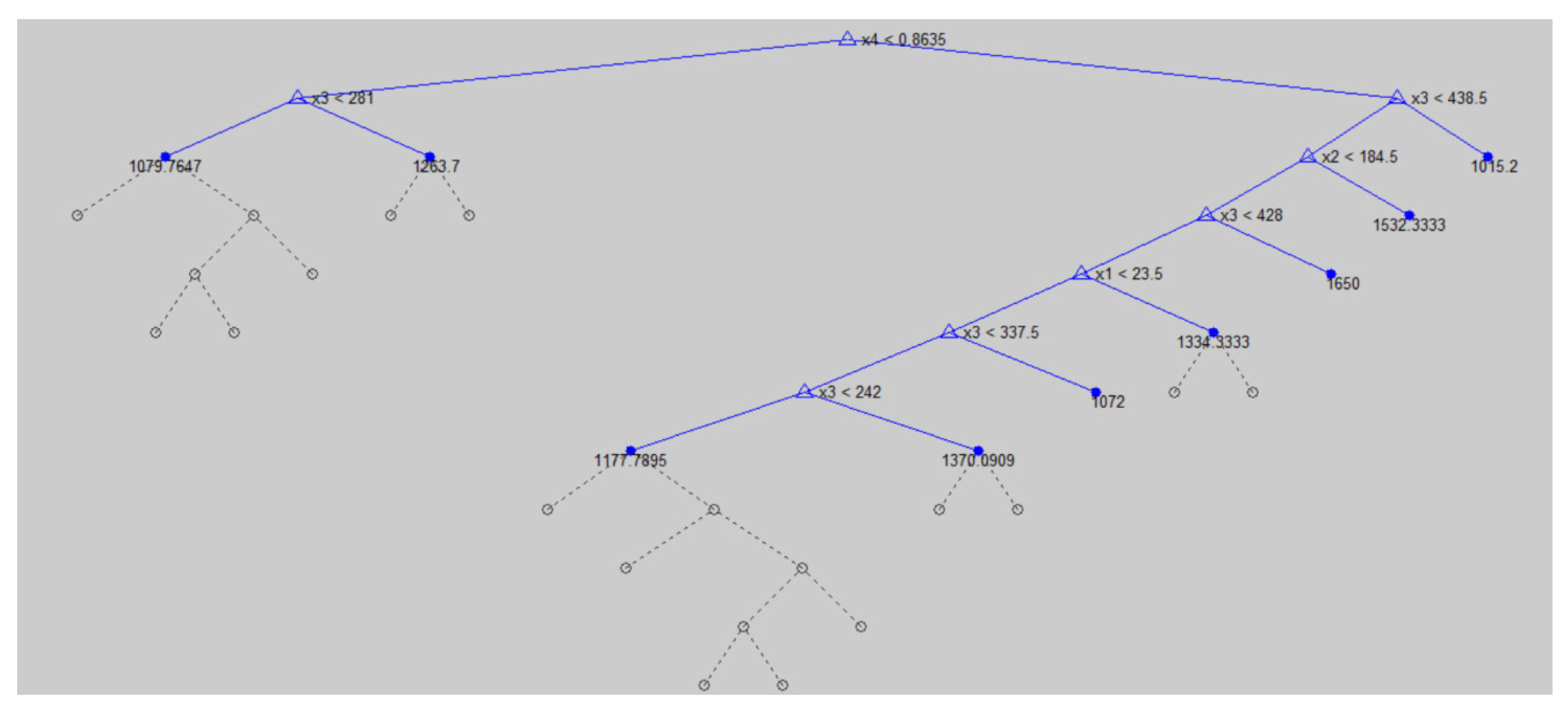
Then, the CABPN tree was pruned by minimizing the cost-complexity measure, for which α was set to 0.001, because in this case most SSE values ranged between 0.001 and 0.01. Finally, the CABPN tree was built, as shown in Figure 7. In total, there were seven BPNs for estimating the cycle times of jobs of the corresponding nodes. The cost-complexity measure of the CABPN tree was 0.06574. After converting to the un-normalized value, the minimal SSE was 3718 h2.
For a comparison, the traditional CART method was also applied to this case, for which MATLAB 2006a was used. The criterion for choosing a split was Gini. In addition, impure nodes must have 10 or more jobs to be split. Subsequently, the CART tree was pruned based on an optimal pruning scheme that first prunes branches contributing to the least improvement in SSE. Finally, the results were shown in Figure 8. The minimal SSE was 2,398,777 h2, much greater than that obtained using the CABPN tree approach. However, such a difference was for the training data.
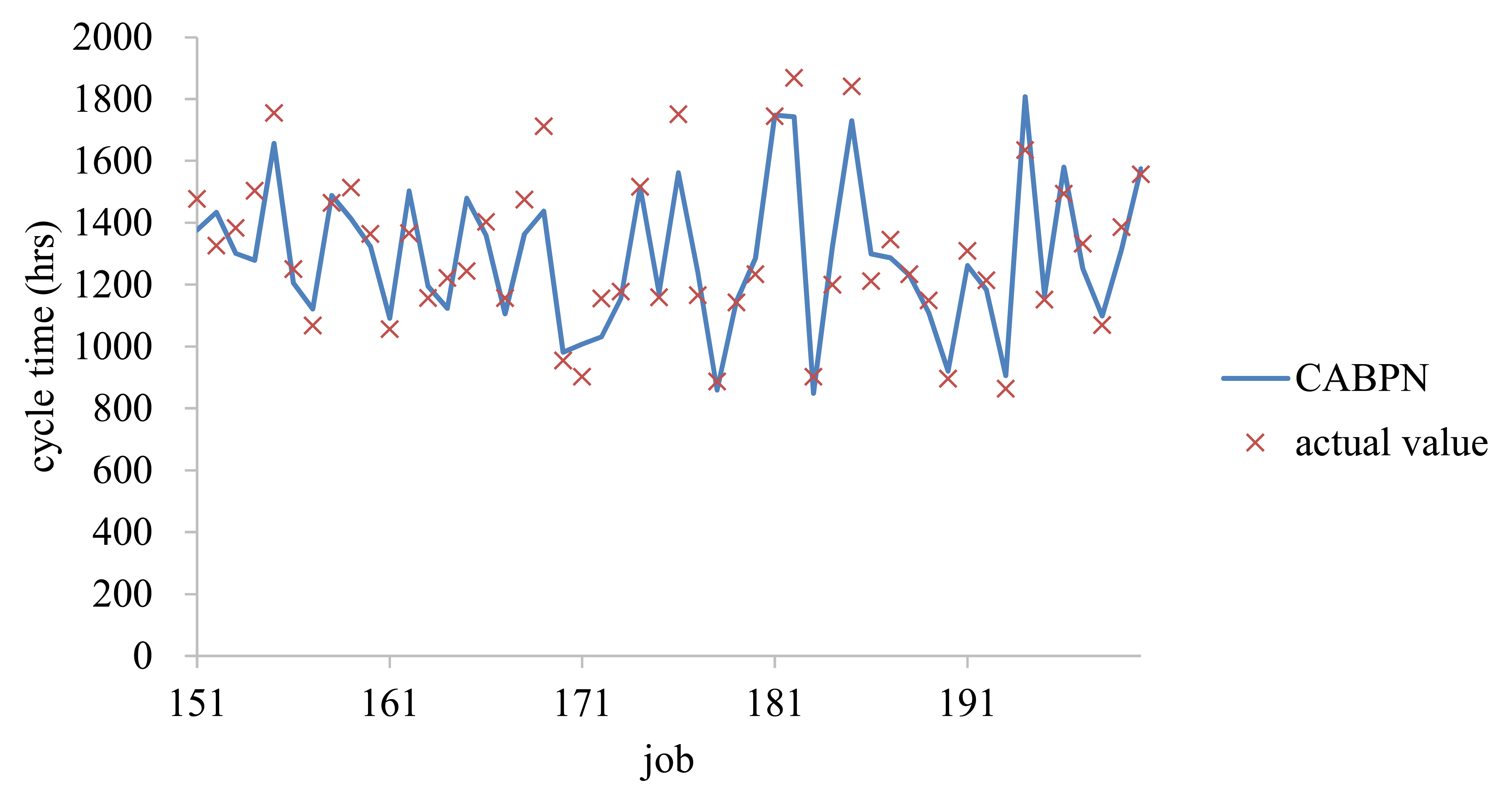
The two approaches were applied to the testing data. The estimation results using the proposed methodology were shown in Figure 9. The performances of CABPN tree and CART were compared in terms of mean absolute error (MAE), mean absolute percentage error (MAPE), and root mean squared error (RMSE):
The results are summarized in Table 6. According to the experimental results,
- (1)
Obviously, the estimation accuracy, measured in terms of MAE, MAPE, or RMSE, using the proposed CABPN tree approach was much better than that by the traditional CART approach. The advantage was the most obvious (up to 23%) in the RMSE regard.
- (2)
On the other hand, the numbers of jobs of nodes in the CABPN tree were summarized in Table 7. Obviously, the numbers of jobs assigned to the two nodes of a branch were close using the proposed methodology (see Figure 10), due to the symmetric property of the SP-IR algorithm. It gave enough examples to train the BPN of each node. In contrast, some nodes in the CART tree, such as node 8, had very few examples (see Table 8).
- (3)
Starting with different initial conditions, a BPN will converge to different results, so does the CABPN tree approach, which means it is likely to further improve the estimation accuracy of the CABPN tree approach in an iterative way or with carefully chosen initial conditions.
- (4)
However, the training time required for the CABPN tree approach was 297 s, much longer than that required for the CART approach (less than 5 s). Obviously, the efficiency of the proposed methodology needs to be improved somehow.
- (5)
A sensitivity analysis was performed to assess the effects of α on the estimation performance of the CABPN tree approach. The results are summarized in Figure 11. Obviously, a large value of α resulted in fewer branches, which was not conducive to the estimation accuracy for such diverse jobs. Conversely, the stopping criterion of the maximum number of nodes has a positive effect (see Figure 12). With more nodes, the estimation accuracy of the CABPN tree approach became better; however, the effects were not unlimited.
- (6)
The CABPN tree approach is computationally more intensive than its counterpart CART. The computation time required for the CABPN tree approach depends on the number of jobs, the size of each BPN (including the number of hidden layers and the number of nodes in each hidden layer), and the stopping criteria of the CABPN tree. It is almost instantaneous to find a feasible solution by changing the weights of the BPN, but it takes time to evolve the solution to the optimal one. In this case, the CABPN tree approach was implemented on a PC with an Intel Dual CPU E2200 2.2 GHz and 2.0G RAM. It took about 3 min to estimate the cycle times of jobs. In contrast, the CART approach took only 15 s. Obviously, there is considerable room for improving the efficiency of the CABPN tree approach.
- (7)
To further elaborate the effectiveness of the proposed methodology, another existing method—the hybrid kM and BPN approach [12]—was also applied to this case to make a comparison, in which the features of a job category were extracted using kM. The results are summarized in Table 9. The proposed methodology also outperformed the kM-BPN approach.
4. Conclusions and Future Research Directions
An innovative combination of CART and BPN is formed in this study to estimate the cycle time of a job in a wafer fabrication factory, which is always considered as one of the most important tasks in controlling a wafer fabrication factory. After embedding an individual BPN into each node of a classification tree, the CABPN tree approach is proposed, so that the cycle times of jobs of the same node will be estimated with the same BPN, instead of a single value as in the traditional CART approach. Such a treatment is expected to improve the estimation accuracy. However, to determine the optimal location of the splitting point on a node is a challenging task. To tackle this issue, the SP-IR algorithm is proposed to generate quite symmetric partitioning results. In this way, most BPNs can be trained with enough examples.
The effectiveness of the proposed CABPN tree approach was evaluated with a real case from a DRAM manufacturing factory. According to the experimental results,
- (1)
The estimation accuracy, measured in terms of MAE, MAPE, or RMSE, was significantly improved after applying the CABPN tree approach;
- (2)
On the other hand, there is considerable room for improving the efficiency of the CABPN tree approach, owing to the extensive BPN learning;
- (3)
The estimation accuracy of the CABPN tree approach can be further improved in an iterative way or with carefully chosen initial conditions.
The symmetric property of the SP-IR algorithm aims to reserve enough examples for each node, however, may cause the CABPN tree to be trapped in the local optimum. This issue can be investigated in a future study.
Acknowledgments
This work was supported by National Science Council of Taiwan.
Conflicts of Interest
The author declares no conflict of interest.
References
- Inoue, T.; Ishii, Y.; Igarashi, K.; Takagi, H.; Muneta, T.; Imaoka, K. Conveyer Belt Model to analyze cycle time conditions in a semiconductor manufacturing line. Proceedings of the IEEE International Symposium on Semiconductor Manufacturing Conference, Tokyo, Japan, 25–27 September 2006; pp. 74–77.
- Wein, L.M. On the relationship between yield and cycle time in semiconductor wafer fabrication. IEEE Trans. Semicond. Manuf. 1992, 5, 156–158. [Google Scholar]
- Kingman, J.F.C. The single server queue in heavy traffic. Math. Proc. Camb. Philos. Soc. 1961, 57, 902–904. [Google Scholar]
- Chen, H.; Harrison, J.M.; Mandelbaum, A.; van Ackere, A.; Wein, L.M. Empirical evaluation of a queueing network model for semiconductor wafer fabrication. Oper. Res. 1988, 36, 202–215. [Google Scholar]
- Pearn, W.L.; Chung, S.L.; Lai, C.M. Due-date assignment for wafer fabrication under demand variate environment. IEEE Trans. Semicond. Manuf. 2007, 20, 165–175. [Google Scholar]
- Chen, T. An effective fuzzy collaborative forecasting approach for predicting the job cycle time in wafer fabrication. Comput. Ind. Eng. 2013, 66, 838–848. [Google Scholar]
- Chen, T. A fuzzy-neural knowledge-based system for job completion time prediction and internal due date assignment in a wafer fabrication plant. Int. J. Syst. Sci. 2009, 40, 889–902. [Google Scholar]
- Chien, C.F.; Hsu, C.Y.; Hsiao, C.W. Manufacturing intelligence to forecast and reduce semiconductor cycle time. J. Intell. Manuf. 2012, 23, 2281–2294. [Google Scholar]
- Chen, T. A hybrid look-ahead SOM-FBPN and FIR system for wafer lot output time prediction and achievability evaluation. Int. J. Adv. Manuf. Technol. 2007, 35, 575–586. [Google Scholar]
- Chen, T. A fuzzy back propagation network for output time prediction in a wafer fab. Appl. Soft Comput. 2003, 2, 211–222. [Google Scholar]
- Chang, P.-C.; Hsieh, J.-C. A neural networks approach for due-date assignment in a wafer fabrication factory. Int. J. Ind. Eng. 2003, 10, 55–61. [Google Scholar]
- Chen, T. An intelligent hybrid system for wafer lot output time prediction. Adv. Eng. Inform. 2007, 21, 55–65. [Google Scholar]
- Chen, T.; Wang, Y.C. An iterative procedure for optimizing the performance of the fuzzy-neural job cycle time estimation approach in a wafer fabrication factory. Math. Probl. Eng. 2013, 2013, 740478:1–740478:15. [Google Scholar]
- Chen, T. A hybrid SOM-BPN approach to lot output time prediction in a wafer fab. Neural Process. Lett. 2006, 24, 271–288. [Google Scholar]
- Breiman, I.; Friedman, J.H.; Olsen, R.A.; Stone, C.J. Classification and Regression Trees; Wadsworth: Pacific Growe, CA, USA, 1984. [Google Scholar]
- Steinburg, D.; Colla, P. Classification and Regression Trees; Salford Systems: San Diego, CA, USA, 1997. [Google Scholar]
- Firoze, A.; Arifin, M.S.; Rahman, R.M. Bangla user adaptive word Speech recognition: Approaches and comparisons. Int. J. Fuzzy Syst. Appl. 2013, 3, 1–36. [Google Scholar]
- Hecht-Nielson, R. Kolmogorov's mapping neural network existence theorem. Proceedings of the First IEEE International Joint Conference on Neural Networks, San Diego, CA, USA, 21–24 June 1987; pp. 11–14.
- Rogers, L.L.; Dowla, F.U. Optimization of groundwater remediation using artificial neural networks with parallel solute transport modeling. Water Resour. Res. 1994, 30, 457–481. [Google Scholar]


| Method | Classifier | Estimation method | Easiness to use | Accuracy |
|---|---|---|---|---|
| BPN [11] | – | BPN | Easy | Moderate |
| SOM-BPN [14] | SOM | BPN | Moderate | High |
| Pearn et al. [5] | – | Gamma Distribution Fitting | Easy | Low |
| SOM-FBPN [9] | SOM | FBPN | Difficult | High |
| kM-FBPN [12] | kM | FBPN | Difficult | High |
| PCA-CART [6] | PCA-CART | CART | Easy | Moderate |
| CABPN tree | SP-IR | BPN | Easy | High |
| Method | Cycle times of jobs of a category | Tree splitting method | Regression type | Regression method |
|---|---|---|---|---|
| CART | the same | Gini, etc. | Linear | LR |
| CABPN tree | Different | the SP-IR algorithm | Nonlinear | BPN |
| j | xj1 | xj2 | N(CTj) |
|---|---|---|---|
| 1 | 0.100 | 0.391 | 0.100 |
| 2 | 0.112 | 0.677 | 0.176 |
| 3 | 0.575 | 0.440 | 0.582 |
| 4 | 0.546 | 0.900 | 0.546 |
| 5 | 0.304 | 0.100 | 0.288 |
| 6 | 0.305 | 0.466 | 0.436 |
| 7 | 0.232 | 0.716 | 0.267 |
| 8 | 0.861 | 0.895 | 0.795 |
| 9 | 0.900 | 0.672 | 0.900 |
| 10 | 0.720 | 0.286 | 0.511 |
| j | xj1 | xj2 | xj3 | xj4 | CTj |
|---|---|---|---|---|---|
| 1 | 24 | 175 | 441 | 97% | 863 |
| 2 | 23 | 154 | 256 | 97% | 1342 |
| 3 | 23 | 171 | 45 | 87% | 956 |
| 4 | 23 | 183 | 466 | 85% | 1391 |
| 5 | 23 | 163 | 90 | 100% | 1153 |
| 6 | 24 | 181 | 332 | 89% | 1321 |
| … | |||||
| 198 | 23 | 181 | 68 | 98% | 1099 |
| 199 | 22 | 168 | 206 | 89% | 1314 |
| 200 | 23 | 164 | 261 | 91% | 1575 |
| j | xj1 | xj2 | xj3 | xj4 | CTj |
|---|---|---|---|---|---|
| 1 | 0.670 | 0.609 | 0.853 | 0.786 | 0.105 |
| 2 | 0.448 | 0.128 | 0.500 | 0.795 | 0.501 |
| 3 | 0.431 | 0.504 | 0.100 | 0.449 | 0.181 |
| 4 | 0.475 | 0.788 | 0.900 | 0.386 | 0.541 |
| 5 | 0.424 | 0.324 | 0.184 | 0.897 | 0.345 |
| 6 | 0.562 | 0.749 | 0.645 | 0.525 | 0.483 |
| … | |||||
| 198 | 0.545 | 0.737 | 0.144 | 0.817 | 0.300 |
| 199 | 0.348 | 0.450 | 0.406 | 0.536 | 0.477 |
| 200 | 0.437 | 0.346 | 0.511 | 0.584 | 0.692 |
| Method | MAE | MAPE | RMSE |
|---|---|---|---|
| CART | 97 | 8.0% | 126 |
| CABPN Tree | 75 | 5.7% | 97 |
| Node # | 1 | 2 | 3 | 4 | 5 | 6 | 7 |
|---|---|---|---|---|---|---|---|
| No. of jobs | 40 | 17 | 21 | 20 | 14 | 21 | 17 |
| Node # | 1 | 2 | 3 | 4 | 5 | 6 | 7 | 8 | 9 |
|---|---|---|---|---|---|---|---|---|---|
| No. of Jobs | 27 | 16 | 37 | 18 | 10 | 29 | 2 | 5 | 6 |
| Method | MAE | MAPE | RMSE |
|---|---|---|---|
| kM-BPN | 82 | 6.3% | 101 |
| The proposed methodology | 75 | 5.7% | 97 |
© 2014 by the authors; licensee MDPI, Basel, Switzerland. This article is an open access article distributed under the terms and conditions of the Creative Commons Attribution license ( http://creativecommons.org/licenses/by/3.0/).
Share and Cite
Chen, T. The Symmetric-Partitioning and Incremental-Relearning Classification and Back-Propagation-Network Tree Approach for Cycle Time Estimation in Wafer Fabrication. Symmetry 2014, 6, 409-426. https://doi.org/10.3390/sym6020409
Chen T. The Symmetric-Partitioning and Incremental-Relearning Classification and Back-Propagation-Network Tree Approach for Cycle Time Estimation in Wafer Fabrication. Symmetry. 2014; 6(2):409-426. https://doi.org/10.3390/sym6020409
Chicago/Turabian StyleChen, Toly. 2014. "The Symmetric-Partitioning and Incremental-Relearning Classification and Back-Propagation-Network Tree Approach for Cycle Time Estimation in Wafer Fabrication" Symmetry 6, no. 2: 409-426. https://doi.org/10.3390/sym6020409