Reduction by Lie Group Symmetries in Diffeomorphic Image Registration and Deformation Modelling

Abstract

We survey the role of reduction by symmetry in the large deformation diffeomorphic metric mapping framework for registration of a variety of data types (landmarks, curves, surfaces, images and higher-order derivative data). Particle relabelling symmetry allows the equations of motion to be reduced to the Lie algebra allowing the equations to be written purely in terms of the Eulerian velocity field. As a second use of symmetry, the infinite dimensional problem of finding correspondences between objects can be reduced for a range of concrete data types, resulting in compact representations of shape and spatial structure. Using reduction by symmetry, we describe these models in a common theoretical framework that draws on links between the registration problem and geometric mechanics. We outline these constructions and further cases where reduction by symmetry promises new approaches to the registration of complex data types.

1. Introduction

Registration, the task of establishing correspondences between multiple instances of objects, such as images, landmarks, curves and surfaces, plays a fundamental role in a range of computer vision applications, including shape modelling [1], motion compensation and optical flow [2], remote sensing [3] and medical imaging [4]. In the subfield of computational anatomy, establishing inter-subject correspondences between organs allows the statistical study of organ shape and shape variability [5]. Examples of the fundamental role of registration include quantifying developing Alzheimer’s disease by establishing correspondences between brain tissue at different stages of the disease [6]; measuring the effect of chronic obstructive pulmonary disease on lung tissue after removing variability caused by the respiratory process [7]; and correlating the shape of the hippocampus to schizophrenia after inter-subject registration [8].

In this paper, we survey the role of reduction by symmetry in diffeomorphic registration and deformation modelling, linking symmetry as seen from the field of geometric mechanics with the image registration problem. All of our calculations will be formal and void of functional analytic detail, although citations will be used when available. We focus on large deformations modelled in subgroups of the group of diffeomorphic mappings on the spatial domain in the context of large deformation diffeomorphic metric mapping (LDDMM) [1,9–11]. Connections with geometric mechanics [12,13] have highlighted the role of symmetry, and properties that were previously known to be connected with the specific data types have been described in a common theoretical framework [14]. We wish to describe these connections in a form that highlights the role of symmetry and points towards future applications of the ideas.

1.1. Symmetry and Information

One of the main reasons symmetry is useful in data analysis and numerics is its ability to reduce the complexity of information that represents data. Lower information complexity can lead to more stable statistical analysis and the reduced need of computational resources.

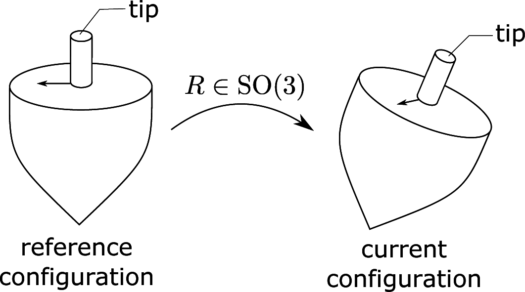
As a toy example, consider a spinning top. Upon choosing a reference configuration, the orientation of the top is given by a rotation matrix, i.e., an element R ∈ SO(3) (see Figure 1). To describe the direction of the tip of the top, it suffices to provide the orientation matrix R. However, R is contained in SO(3), a three-dimensional space, while the space of possible directions is the two-sphere, S², which is only of dimension two. Therefore, providing the full matrix R is an over-representation of the tip direction. It suffices to solely provide the vector R · k ∈ S² where k = (0, 0, 1) is the direction of the tip in a reference configuration. Note that if $\tilde{R}\cdot \mathrm{k}=\mathrm{k}$, then $R\cdot \mathrm{k}=R\cdot \tilde{R}\cdot \mathrm{k}$. Therefore, given only the direction k′ = R · k, we can only reconstruct R up to an element $\tilde{R}$, which preserves k. The subgroup of rotations that preserve k can be identified with SO(2). Specifically, this identification comes from perceiving a rotation about k as a rotation of the plane, which is perpendicular to k. This insight allows us to express the space of directions S² as a homogeneous space S² ≡ SO(3)/SO(2). In terms of information, we can cartoonishly express this by:

$$“\text{orientation}”=“\text{direction of tip}”+“\text{orientation around the tip}”$$

This picture is typical for many group quotients. Generally speaking, if X is a manifold and G acts freely and properly on X, then:

$$\text{dim}(X)=\text{dim}(X/G)+\text{dim}(G)$$

When X is infinite dimensional, this formula is less insightful. However, X/G is smaller than X in that there exists a surjective map from X to X/G with non-trivial level sets. Reduction by symmetry can be implemented when a problem posed on X has G symmetry and can be rewritten as a problem posed on X/G. As X/G is smaller than X, reduction by symmetry can yield more stable subsequent statistical analysis of observed data and more tractable algorithms, as will be shown later in the article. This reduction is particularly dramatic when dim(X) = ∞ and dim(X/G)<∞.

1.2. Symmetry in Registration

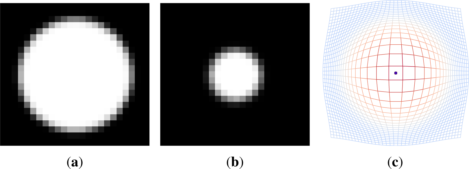
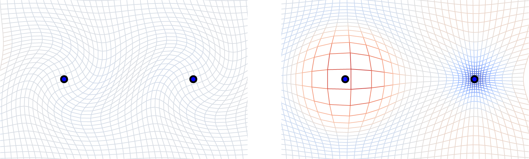
Registration of objects contained in a spatial domain, e.g., the volume to be imaged by a scanner, can be formulated as the search for a deformation that transforms both domain and objects to establish an inter-object match. The data available when solving a registration problem is generally insufficient for determining the displacement of every point of the domain. This is the case when images to be matched have areas of constant intensity and no derivative information can guide the registration. For example, the “best” deformation for matching the two discs in Figure 2 is ambiguous, except at the boundary of the discs, where the images are non-constant. Similarly, when 3D shapes are matched based on the similarity of their surfaces, the deformation of the interior cannot be derived from the available information. In these cases, the deformation model is over-complete, and a range of deformations can provide equally adequate matches for the data. The registration problem or the registration cost-function is thus symmetric with respect to the subset of transformations just described. When the deformation model is a Lie group, the deformations for which the registration is symmetric form a subgroup. The quotient by this subgroup of symmetries of the registration cost-function can provide vastly more compact representations. This situation arises in several cases with the LDDMM framework: when registering images, only displacements orthogonal to the level lines of an image are needed, and when registering shapes, the information left in the quotient is supported on the shape surface only.

1.3. Content and Outline

Although a degree of comfort with differential geometry will be assumed, it is the aim of this paper to make the role of symmetry in registration and deformation modelling clear to the non-expert in geometric mechanics and symmetry groups in image registration. We begin the paper by presenting the background for the registration problem and the large deformation approach before outlining some necessary notions from differential geometry. For more information on the Riemannian geometry behind the LDDMM approach to image registration, we refer the reader to [5]. We continue by describing how reduction by symmetry leads to an Eulerian formulation of the equations of motion when reducing to the Lie algebra. The symmetry of dissimilarity measures allows additional reductions, and we use isotropy subgroups to reduce the complexity of the registration problem further. Lastly, we survey the effect of symmetry in a range of concrete registration problems. The paper ends with concluding remarks.

2. Registration

The registration problem consists of finding correspondences between objects that are typically point sets (landmarks), curves, surfaces, images or more complicated spatially-dependent data, such as diffusion weighted images (DWI). The problem can be approached by letting M be a spatial domain containing the objects to be registered. M can be a compact finite dimensional differentiable manifold without boundary or ℝ^d itself with d = 2, 3. It is common to consider manifolds with boundaries, as well. In such cases, care must be taken with regards to boundary conditions. For example, vector-fields must be tangential to the boundary. Here, we consider only manifolds without a boundary.

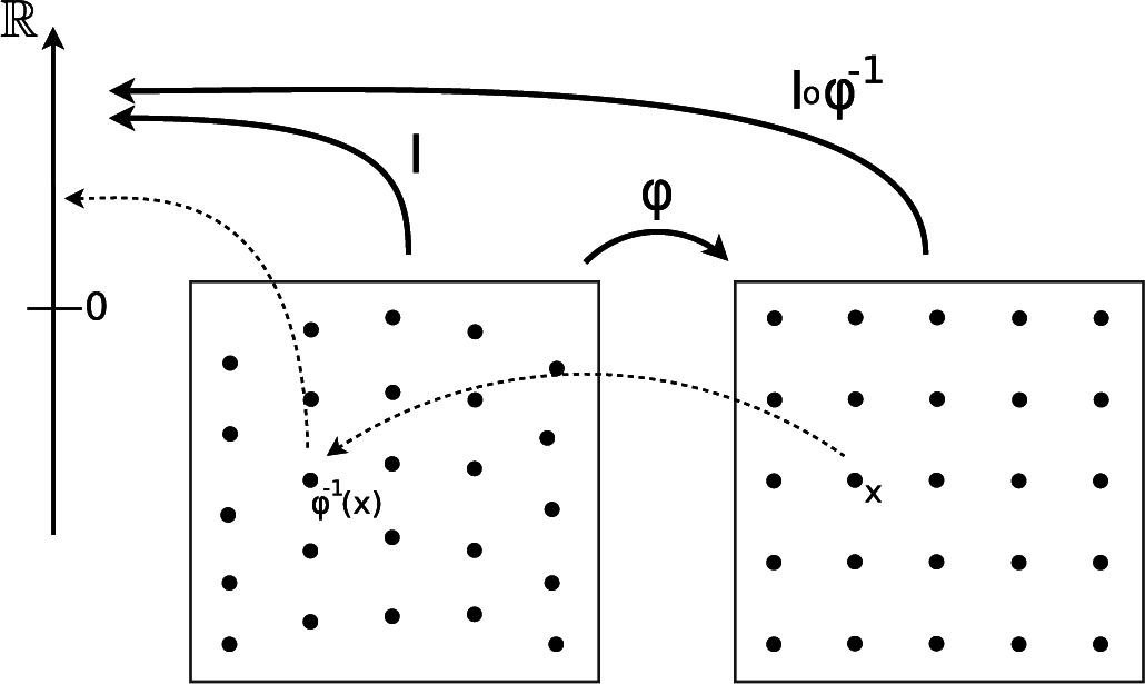
A map φ : M → M can deform or warp the domain by mapping each x ∈ M to φ(x). The deformation encoded in the warp will apply to the objects in M, as well as the domain itself. For example, if the objects to be registered consist of point sets {x₁,…, x_N}, x_i ∈ M, the set will be mapped to {φ(x₁),…, φ(x_N)}. For surfaces S ⊂ M, φ similarly results in the warped surface φ(S). Because those operations are associative, the mapping φ acts on {x_i} or S, and we write φ · {x_i} and φ · S for the warped objects. An image is a function I : M → ℝ, and φ acts on I as well, in this case by composition with its inverse φ · I = I ○ φ⁻¹; see Figure 3. For this, φ must be is invertible, and commonly, we restrict to the set of invertible and differentiable mappings Diff(M). For various other types of data objects, the action of a warp on objects can be defined in a manner similar to that of point sets, surfaces and images. This fact relates a range registration problems to the common case of finding appropriate warps φ, which bring the objects into correspondence. Different shape instances can be realized by letting warps act on a base shape, and a class of shape models can thereby be obtained by using deformations as shape representations [1].

The search for appropriate warps can be formulated in a variational formulation with an energy:

$$E(\phi )=R(\phi )+F(\phi )$$

(1)

where F is a dissimilarity measure of the difference between the deformed objects and R is a regularization term that penalizes unwanted properties of φ, such as spatial irregularity. If two objects o₁ and o₂ are to be matched, F can take the form F (φ · o₀, o₁) using the action of φ on o₀; for image matching, an often used dissimilarity measure is the L²-difference or sum of square differences (SSD) having the form $F(\phi \cdot I_0,I_1)={\displaystyle {\int }_M|I_0\circ {\phi }^{-1}(x)-I_1(x){|}^{2}dx}$.

The regularization term can take various forms often modelling physical properties, such as elasticity [15], and derivatives of φ are often penalized to ensure smoothness. For some choices of R, existence and analytical properties of minimizers of Equation (1) have been derived [16]; however, in general, it is difficult to ensure that solutions are diffeomorphic by penalizing φ in itself. The free-form-deformation (FFD; [17]) and related approaches model the deformation by a displacement vector field u on M = ℝ^d, so that φ(x) = x + u(x). Smoothness is here ensured by the choice of basis functions, e.g., B-splines, or by applying a regularization term on u. Smooth and invertible mappings can be obtained by integrating flows [9,11] to obtain one-parameter families or paths of mappings φ_t, t ∈ [0, 1]. The warp φ₀ at t = 0 is here the identity mapping id ∈ Diff(M), and the dissimilarity is measured at the endpoint φ₁. The time evolution of φ_t can be described by the differential equation:

$$\frac{d}{dt}{\phi }_t(x)=u_t({\phi }_t(x))$$

(2)

with the flow field u_t being a vector field on M. Numerically, the map φ can be represented by how it maps a finite set of points, and a numerical scheme might simply implement Euler-integration on each point, i.e., “x_i+1 ↦ x_i + h · u_t(x_i)” with time-step size 0 < h ≪ 1. A relaxation of this idea is now a standard method in optical flows [18]. The space of flow fields is denoted by V. In the LDDMM [1] framework, the regularization is applied to the flow field and integrated over time giving the energy:

$$E(\phi )={\displaystyle {\int }_0^1||u_t|{|}_V^{2}dt+F({\phi }_1)}$$

(3)

Here, the time-dependent diffeomorphism φ_t is related to u_t through Equation (2). If the norm ‖·‖_V that measures the irregularity of u_t is sufficiently strong (e.g., H^k with $k>\frac{d}{2}+1$), then φ_t will be a diffeomorphism for all t [19]. This approach thus gives a direct way of enforcing properties of the generated warp: instead of regularizing φ directly, the analysis is lifted to a normed space V that is much easier control. The energy E in Equation (3) has the same minimizers as the geometric formulation of LDDMM used in the next section.

Direct approaches to solving the optimization problem in Equation (3) must handle the fact that the problem of finding a warp is now expanded to that of finding a time-dependent family of warps. This is a huge increase in dimensionality. This formulation of registration is thus very difficult to represent numerically and to optimize and analyse statistically. For several data types, it has been shown how optimal paths for Equation (3) have specific properties that reduce the dimensionality of the problem, making practical solutions feasible. In the next section, we outline the geometric framework that is needed when we, in the later sections, use reduction by symmetry to describe these data-dependent results in a common theoretical framework.

3. Notions from Differential Geometry

In this section, we will introduce a number of notions from differential geometry in a fairly informal manner. We will use conventions from [20,21] where a more rigorous understanding of differential geometry can be found.

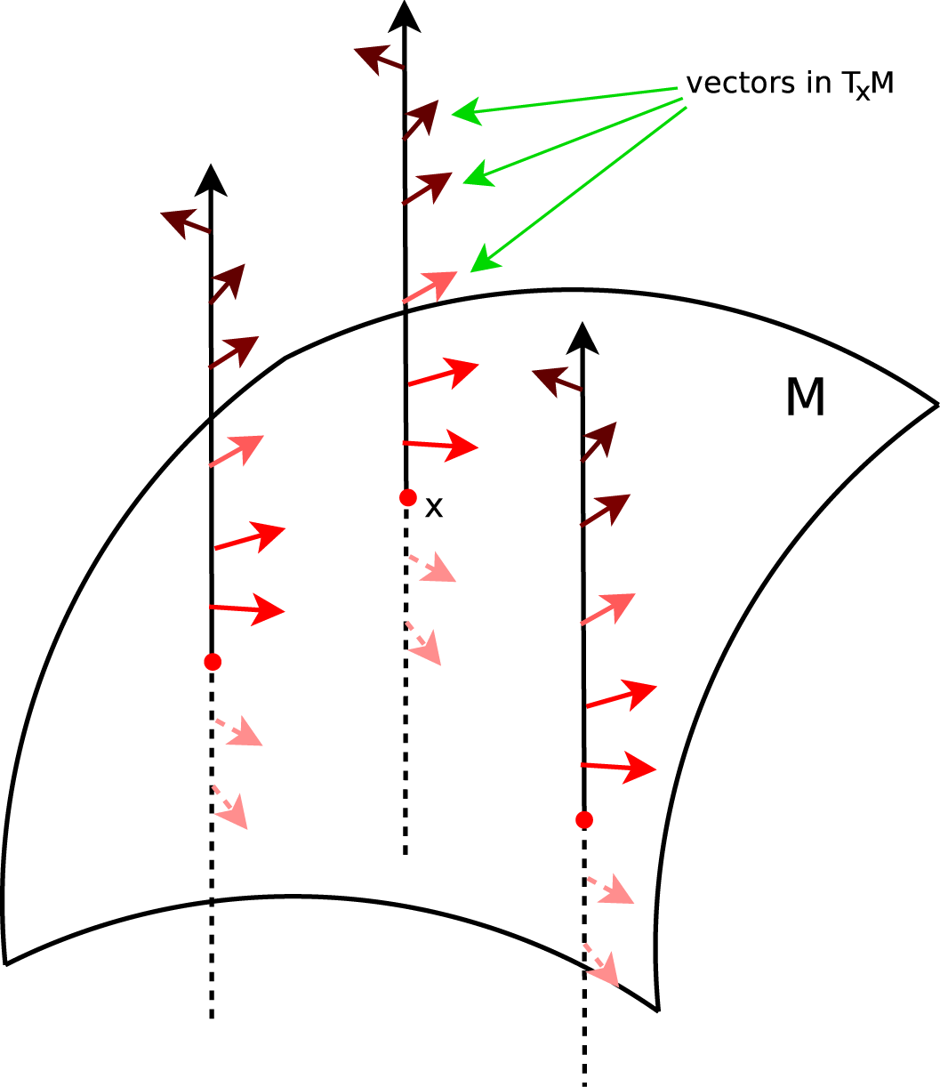
We will assume that the reader has at least an intuitive picture of the notion of a smooth manifold M. For the purpose of this paper, M will either be assumed to be compact without a boundary or ℝⁿ. The tangent bundle of M is the space of velocity vectors tangential to M. Notationally, the tangent bundle of M, denoted TM, is the set of pairs (x, v) where x ∈ M and v is a vector tangential to M at the point x (see Figure 4). A vector-field is a continuous map u : M → TM, such that u(x) ∈ TM is a vector above x for all x ∈ M. We will denote the space of vector-fields by $\mathfrak{X}(M)$.

Given a vector-field $u\in \mathfrak{X}(M)$, we may consider the initial value problem:

$$\{\begin{array}{l}x(0)=x_0\hfill \\ \frac{dx}{dt}=u(x(t))\hfill \end{array}$$

for t ∈ [0, 1]. Given an initial condition x₀, the point x₁ = x(1) given by solving this initial value problem is uniquely determined if it exists. Under many circumstances (e.g., if M is compact or if M = ℝ^d and ‖u(x)‖ grows sub-linearly), an x₁ exists for each x₀, and there is a continuous invertible map ${\Phi }_t^u:x_0\in M\mapsto x_1\in M$, which we call the flow of u. Given a time-dependent vector-field, $u_t\in \mathfrak{X}(M)$ for t ∈ [0, 1], we can consider the initial value problem with $\frac{dx}{dt}=u_t(x(t))$. This will yield a flow map, ${\Phi }_{t_0,t_1}^u$ which is the flow from time t = t₀ to t = t₁. If u_t is smooth, the flow map will be smooth, as well, in particular a diffeomorphism. We denote the set of diffeomorphisms by Diff(M).

Conversely, let φ_t ∈ Diff(M) be a time-dependent diffeomorphism. For any x ∈ M, we observe that φ_t(x) is a curve in M. If this curve is differentiable we may consider its time-derivative, $\frac{d{\phi }_t}{dt}(x)\in TM$, which is a vector above the point φ_t(x) ∈ M. From these observations, it follows that $\frac{d{\phi }_t}{dt}[{\phi }_t^{-1}(x)]$ is a vector above x. Therefore, the map u_t : M → TM, given by $u_t\left(x\right):=\left(\frac{d}{dt}{\phi }_t\right)\left[{\phi }_t^{-1}\left(x\right)\right]$, is a vector-field called the Eulerian velocity field of φ_t.

As will be described shortly, the Eulerian velocity field contains less data than $\frac{d{\phi }_t}{dt}$. This reduction in data can be viewed from the perspective of symmetry. Given any ψ ∈ Diff(M), the curve φ_t can be transformed to the curve φ_t ○ ψ. We observe that:

$$\begin{array}{l}{u}_t:=\frac{d{\phi }_t}{dt}\circ {\phi }_t^{-1}=\frac{d{\phi }_t}{dt}\circ \psi \circ {\psi }^{-1}\circ {\phi }_t^{-1}\\ =\left(\frac{d}{dt}\left({\phi }_t\circ \psi \right)\right)\circ {\left({\phi }_t\circ \psi \right)}^{-1}\end{array}$$

Thus, φ_t and φ_t ○ ψ both have the same Eulerian velocity fields. In other words, the Eulerian velocity field, u_t, is invariant under particle relabellings. More precisely, we may view Diff(M) as a manifold in its own right, and view $\frac{d{\phi }_t}{dt}$ as a vector in the infinite-dimensional tangent bundle T Diff(M) above the “point” φ_t ∈ Diff(M). Thus, the vector $\frac{d{\phi }_t}{dt}$ contains both velocities and a base diffeomorphism φ_t. Given u_t and φt, we can reconstruct $\frac{d{\phi }_t}{dt}$ via $\frac{d{\phi }_t}{dt}=u_t\circ \phi t.$ As has been shown, we can also construct u_t from $\frac{d{\phi }_t}{dt}$ by its own definition. However, we cannot reconstruct $\frac{d{\phi }_t}{dt}$ from u_t, which is why u_t contains less data.

Finally, we will denote some linear operators on the space of vector-fields. Let Φ ∈ Diff(M), and let $u\in \mathfrak{X}(M)$. The push-forward of u by Φ is the vector-field given by:

$${\Phi }_{*}u(x):=D\Phi {|}_{{\Phi }^{-1}(x)}\cdot u({\Phi }^{-1}(x))$$

In local coordinates (x¹,…, xⁿ), this looks like:

$${[{\Phi }_{*}u]}^i(x)={\displaystyle \sum _{j=1}^n\left({\partial }_j{|}_{{\Phi }^{-1}(x)}{\Phi }^i\right)u^j\left({\Phi }^{-1}\left(x\right)\right)}$$

By inspection, we see that Φ_∗ is a linear operator on $\mathfrak{X}(M)$. One can view Φ_∗u as “u in a new coordinate system”, because any geometric property of u is also inherited by Φ_∗u. For example, if S is invariant under u, then Φ(S) is invariant under Φ_∗u. We define the pull-back by Φ^∗u := (Φ⁻¹)_∗u. Note that Φ^∗(Φ_∗(u)) = u.

As Φ_∗ is a linear operator, a well-defined operator exists, which is dual to Φ_∗. Let $\mathfrak{X}{(M)}^{*}$ denote the dual space to $\mathfrak{X}(M)$, i.e., the set of linear maps $\mathfrak{X}(M)\to ℝ$, which are continuous with respect to a chosen vector-space topology on $\mathfrak{X}(M)$. Given $m\in \mathfrak{X}{(M)}^{*}$, we define ${\Phi }_{\ast }m\in \mathfrak{X}{(M)}^{*}$ by the identity:

$$\langle {\Phi }_{*}m,{\Phi }_{*}u\rangle :=\langle m,u\rangle$$

(4)

for all $u\in \mathfrak{X}(M)$, where 〈m, u〉 denotes the evaluation of m on v. We can define Φ^∗m := (Φ⁻¹)_∗m, which yields the identity:

$$\langle {\Phi }^{*}m,u\rangle =\langle m,{\Phi }_{*}u\rangle$$

In local coordinates, we may represent m as a one-form density, given by m_i(x)dxⁱ⊗(dx¹∧…∧dxⁿ) with components m₁(x),…, m_n(x). In this local coordinate description, the i-th component of the push-forward looks like:

$${[{\Phi }_{\ast }m]}_i(x):=\det (D{\Phi }^{-}{}^1){|}_x{\partial }_i{\Phi }^j{|}_{{\Phi }^{-1}(x)}\cdot m_j({\Phi }^{-1}(x))$$

Finally, we define the Lie derivative. Let $w\in \mathfrak{X}(M)$. The Lie derivative operator, with respect to w, is the linear operator ${\pounds }_w:\mathfrak{X}(M)\to \mathfrak{X}(M)$ defined by:

$${\pounds }_w[u]={\frac{d}{dϵ}|}_{ϵ=0}{({\Phi }_{ϵ}^w)}^{*}u$$

Again, as £_w is a linear operator on $\mathfrak{X}(M)$, we can define a dual operator on $\mathfrak{X}{(M)}^{*}$. If $m\in \mathfrak{X}{(M)}^{*}$, we can define ${\pounds }_w[m]\in \mathfrak{X}{(M)}^{\ast }$£_w[m] ∈ X(M)^∗ by the equation:

$$\langle {\pounds }_w[m],u\rangle +\langle m,{\pounds }_w[u]\rangle =0$$

(5)

for all $u\in \mathfrak{X}(M)$.

We conclude the section with a table of notation for the reader’s convenience, see

Table 1. Notation.

Notion	Notation
manifold	M
tangent bundle	TM
the group of diffeomorphisms	Diff(M)
the space of vector-fields	$\mathfrak{X}(M)$
the push-forward of u u$\mathfrak{X}$(M) with respect to Φ ∈ Diff(M)	Φ*u
the push-forward of m ∈ $\mathfrak{X}$(M)* with respect to Φ 2∈ Diff(M)	Φ*m
The Lie derivative (w.r.t. u ∈ $\mathfrak{X}$(M))	${\mathrm{L}}_u$
the dual space to $\mathfrak{X}$(M)	$\mathfrak{X}$(M)*
Evaluation of m ∈ $\mathfrak{X}$(M)* on u ∈ $\mathfrak{X}$(M)	〈m, u〉

.

4. Reduction by Symmetry in LDDMM

In this section, we will present necessary conditions satisfied by local extremizers of the variational problem Equation (3). The resulting conditions will first involve the computation of a curve in Diff(M), as well as its time-derivative in T Diff(M). We then invoke a Diff(M) symmetry of the problem to reduce this computation to a computation on $\mathfrak{X}(M)$ instead of T Diff(M) ≅ Diff(M) ×$\mathfrak{X}(M)$. Secondly, we describe how the symmetry of the dissimilarity measure allows further reductions.

4.1. Reduction to the Lie Algebra

The variational formulation Equation (3) of LDDMM is equivalent to minimizing the energy:

$$E=d(id,\phi )+F(\phi )$$

(6)

where d : Diff(M) × Diff(M) → ℝ is a Riemannian distance metric on Diff(M) induced by the norm ‖·‖_V, id is the identity diffeomorphism, and F : Diff(M) → ℝ is a dissimilarity measure, i.e., a function measuring the disparity between the deformed template and the target object.

Example 1. Given images I₀, I₁ ∈ L²(M), we consider the dissimilarity measure:

$$F(\phi )=||(I_0\circ {\phi }^{-1})-I_1|{|}_{L^2(M)}^2$$

In this article, we will consider the metric on connected components of Diff(M) given by:

$$d({\phi }_0,{\phi }_1)=\underset{\underset{{\Phi }_{0,1}^v\circ {\phi }_0={\phi }_1}{u\in C^0([0,1]\mathfrak{X}(M))}}{\inf }\left({\displaystyle {\int }_0^1||u_t||dt}\right)$$

where u_t denotes a one-parameter family of vector fields and ‖·‖ is a norm on $\mathfrak{X}(M)$, the Lie algebra of Diff(M). The norm is generally assumed to be admissible, i.e., embedded in $C_0^1(M,{ℝ}^n{}^{+k})$ for sufficiently large k, so that a constant C exists satisfying ‖u‖ ≥ C‖u‖_1,∞ for all u ∈ X(M) ([1], Chapter 9). In the case where M ≠ ℝⁿ, we can define ‖u‖_1,∞ chart-wise by a partition of unity (e.g., see the construction of H^k norms on M in [22]) or intrinsically in terms of the Riemannian gradient. Both choices would yield identical topologies, and so, this choice has no significance as far as the article is concerned. From now on, we will overload notation and let $\mathfrak{X}(M)$ denote the set of C^k vector fields with finite norm. For finite k, this makes $\mathfrak{X}(M)$ a Banach space, and it breaks the Lie algebra structure. The consequences of this breakage will not be explored here, and we will continue to treat $\mathfrak{X}(M)$ formally as a Lie algebra. We will later be using the space of homeomorphisms generated by $\mathfrak{X}(M)$, which is a subspace of C^k-diffeomorphisms. Again, we will overload the notation and call this space Diff(M), even though this is usually reserved for smooth diffeomorphisms. In the case where M = ℝ^d, we assume that our norm is such that decay conditions at infinity for $u\in \mathfrak{X}(M)$ arise naturally as a result of requiring the norm to be finite. If ‖·‖ is induced by an inner-product, the inner-product is formally a Riemannian metric on Diff(M) given by:

$${\Vert \frac{d{\phi }_t}{dt}\Vert }_{{\varphi }_t}^2:={\Vert \frac{d{\phi }_t}{dt}\circ {\phi }_t^{-1}\Vert }^2$$

and d is the Riemannian distance with respect to this metric. The norm is often defined in terms of an operator $P:\mathfrak{X}(M)\to \mathfrak{X}{(M)}^{\ast }$as ‖u‖² = 〈P [u], u〉, and the assumed admissibility implies that $(\mathfrak{X}(M),||·||)$has a reproducible kernel Hilbert space structure (RKHS; [1], Chapter 8). For example, we could consider M = ℝ, $P=dx\otimes (1-{\partial }_x^2)$, and the vector-field u(x) = exp(−|x|) is mapped to the one-form density dx ⊗ δ, where δ is the Dirac delta distribution (see [23]. In particular, in the case that M = ℝⁿ, a matrix-valued kernel function K : ℝⁿ × ℝⁿ → ℝ^n×n exists satisfying the reproducing property 〈P [K(·, x)a], u〉 = a^T u(x) for all x ∈ ℝⁿ and a ∈ Rⁿ (see [24]). We will denote RKHSs by V and the norms by ‖·‖_V.

Given P, minimizers of E Equation (6) must satisfy:

$$\{\begin{array}{l}{m}_t={({\Phi }_{t,1}^{u_t})}_{*}{m}_1=P[u_t]\hfill \\ {\partial }_t{\Phi }_{t,1}^u=-u_t\circ {\Phi }_{t,1}^u\hfill \\ \langle m_1,w\rangle ={\frac{d}{dϵ}|}_{ϵ=0}F({\Phi }_{ϵ}^w\circ {\Phi }_{0,1}^u),\forall w\in \mathfrak{X}(M).\hfill \end{array}$$

(7)

That Equation (7) is a necessary condition satisfied by the minimizers of Equation (6) (under certain analytic assumptions) is stated and proven in [1] (Proposition 11.6) for the case of M = ℝⁿ. The proof is based on the definition of the curve energy Equation (6) as a sum a Riemannian distance d and the dissimilarity measure F. Minimization of the Riemannian distance d yields a search for a geodesic in Diff(M), because geodesics are distance minimizing. The corresponding geodesic equations are given by the first two lines of Equation (7). The term F only penalizes the end-point of the geodesic, and the minimization condition manifests as the third line of Equation (7).

Issues regarding the well-posedness of Equation (7) are non-trivial, because P is merely injective, but not bijective, and so, there is no guarantee that P can be inverted on a given $m_t\in \mathfrak{X}{(M)}^{\ast }$at each time in order to obtain a vector-field $u_t\in \mathfrak{X}(M)$. Fortunately, safety guards for well-posedness are known (e.g., [19], Theorem 1, or [25]).

Using Equation (7) for computational purposes is difficult because Diff(M) is a non-linear infinite dimensional space. Moreover, the dissimilarity measure F only comes into play at time t = 1, and the distance function is an integral over the vector-space $\mathfrak{X}(M)$. It would be beneficial if we could rewrite the extremizers in terms of the Eulerian velocity field u and the flow at t = 1. In fact, this is often the case. One (formally) must take the time-derivative of the term “ ${({\Phi }_{t,1}^u)}_{\ast }m(1)$” and apply Equation (5). Explicitly, this computation is performed as follows. Let $w\in \mathfrak{X}(M)$, and observe:

$$\langle {\partial }_t{m}_t,w\rangle =\langle \frac{d}{dt}{({\Phi }_{t,1}^u)}_{*}m(1),w\rangle =\langle m,\frac{d}{dt}{({\Phi }_{t,1}^u)}^{*}w\rangle =\langle m,{\pounds }_{u_t}[w]\rangle =-\langle {\pounds }_{u_t}[m],w\rangle$$

As w is arbitrary, we find ∂_tm_t + £_ut[m_t] = 0. This allows us to reformulate Equation (7) as:

$$\{\begin{array}{l}{\partial }_t{m}_t+{\pounds }_{u_t}[m_t]=0,m_t=P[u_t]\forall t\in [0,1]\hfill \\ {\frac{d}{dϵ}|}_{ϵ=0}[F({\Phi }_{ϵ}^w\circ {\Phi }_{0,1}^u)]+\langle P[u_1],w\rangle =0,\forall w\in \mathfrak{X}(M)\hfill \end{array}$$

(8)

The advantage of this formulation is that the bulk of the computation occurs on the vector-space $\mathfrak{X}(M)$rather than on the space T Diff(M). Registration algorithms based on Equation (8) differ from the algorithm proposed by Beg et al. in [26]. In [26], a gradient descent on the time-dependent Eulerian vector field u_t is used to minimize the curve energy. The algorithm is posed on the velocity field u_t instead of the momentum field m_t as Equation (8) suggests. The momentum at time t is retrieved by a transport equation similar to the first equation in Equation (7). The evolution Equation (8) effectively allows one to search over the space of initial conditions, $\mathfrak{X}{(M)}^{*}$, rather than over the larger space of curves, C¹([0, 1]; $\mathfrak{X}(M)$).

This reduction of the problem from T Diff(M) given in Equation (7) to the problem over space of vector-fields, $\mathfrak{X}(M)$given in Equation (8) is the first instance of reduction by symmetry. In particular, this corresponds to the fact that the space of vector-fields $\mathfrak{X}(M)$is identifiable as a quotient space:

$$\mathfrak{X}(M)\equiv T\text{Diff}(M)/\text{Diff}(M)$$

Additionally, the map $\left({\phi }_t,\frac{d{\phi }_t}{dt}\right)\in T\text{Diff}(M)\mapsto \frac{d{\phi }_t}{dt}\circ {\phi }_t^{-1}\in \mathfrak{X}(M)$is the quotient projection.

4.2. Isotropy Subgroups

The reduction to dynamics on T Diff(M) to dynamics on $\mathfrak{X}(M)$occurs primarily because the distance function is Diff(M) invariant. However, one cannot completely abandon Diff(M), because the solution requires one to compute the Time 1 flow, ${\Phi }_{0,1}^u$. Fortunately, there is a second reduction, which allows us to avoid computing ${\Phi }_{0,1}^u$in its entirety. This second reduction corresponds to the invariance properties of the dissimilarity measure F. Let G_F ⊂ Diff(M) denote the set of diffeomorphisms, which leave F invariant, i.e.:

$$G_F:=\{\psi \in \text{Diff}(M)|F\left(\phi \circ \psi \right)=F(\phi ),\forall \phi \in \text{Diff}(M)\}$$

One can readily verify that G_F is a subgroup of Diff(M), and so, we call G_F the isotropy subgroup of F.

Having defined G_F, we can now consider the homogeneous space Q = Diff(M)/G_F, which is the quotient space induced by the action of the right composition of G_F on Diff(M). This quotient space is “smaller” in the sense of the amount of data required to describe an element of it. In terms of maps, this can be seen by defining the map φ ∈ Diff(M) ↦q = [φ]_/GF ∈ Q, where [φ]_/GF denotes the equivalence class of φ. We call this mapping the quotient projection, because it sends Diff(M) to Q surjectively. While these notions are theoretically quite complicated, often they manifest less so in practice.

Example 2. In this example, we consider a simple aspect of the landmark matching problem. Let M ⊂ ℝⁿ be the closure of some open set. Let x₁, x₂, y₁, y₂ ∈ M with x₁ ≠ x₂, and consider the dissimilarity measure:

$$F(\phi )=||\phi (x_1)-y_1|{|}^2+||\phi (x_2)-y_2|{|}^2$$

We see that:

$$G_F\equiv \{\psi \in \text{Diff}(M)|\psi (x_1)=x_1,\psi (x_2)=x_2\}$$

and:

$$Q=\text{Diff}(M)/G_F\equiv \{(z_1,z_2)\in M\times M|z_1\ne z_2\}=M\times M-{\mathrm{\Delta }}_{M\times M}$$

where Δ_M×M denotes the diagonal of M × M. The quotient projection is φ ∈ Diff(M) ↦ (φ(x₁), φ(x₂)) ∈ M × M − Δ_M×M

Note that Diff(M) is infinite dimensional, while Q is of dimension 2 dim(M). Two examples of diffeomorphisms contained in G_F are shown in Figure 5.

Example 3. In this example, we consider the matching problem for greyscale images. Let I₀, I₁ ∈ H^k(M) be images. There is a natural action of Diff(M) on H^k given by sending each image I ∈ H^k(M) to I ○ φ ∈ H^k(M). We could consider the matching function F : Diff(M) → ℝ given by:

$$F(\phi )=||(I_0\circ {\phi }^{-}{}^1)-I_1|{|}_{H^k}$$

This function measures the difference between a deformed version of I₀ and a fixed image, I₁. The isotropy subgroup G_F is the group of images that preserve 0₀. Such a diffeomorphism would preserve each of the level lets of I₀, but could permute the points within a given level set.

If one is able to understand Q, then one can use this insight to reformulate the dissimilarity measure F as a function on Q, rather than Diff(M). In particular, there exists a unique function F_Q : Q → ℝ defined by the property F_Q([φ]_/GF ) = F(φ). Again, this is useful in the sense of data, as illustrated in the following example.

Example 4. Consider the dissimilarity measure F of Example 2. The function, F_Q : Q → ℝ is:

$$F_Q(q_1,q_2)=||q_1-y_1|{|}^2+||q_2-y_2|{|}^2$$

Finally, note that Diff(M) acts upon Q by the left action:

$${[\phi ]}_{G_F}\in \text{Diff}(M)/G_F\stackrel{\psi \in \text{Diff}(M)}{\mapsto }{[\psi \circ \phi ]}_{/G_F}\in \text{Diff}(M)/G_F$$

Usually, we will simply write ψ · q for the action of ψ ∈ Diff(M) on a given q ∈ Q. This means that $\mathfrak{X}(M)$acts upon Q infinitesimally, as it is the Lie algebra of Diff(M).

Example 5. Consider the setup of Example 2. Here, Q = M × M − Δ_M×M, and the left action of Diff(M) is given by:

$$\psi \cdot (q_1,q_2)=(\psi (q_1),\psi (q_2))$$

for ψ ∈ Diff(M) and q = (q₁, q₂) ∈ Q. The infinitesimal action of$u\in \mathfrak{X}(M)$on Q is:

$$u\cdot (q_1,q_2)=(u(q_1),u(q_2))\in T_{q}Q$$

These constructions allow us to rephrase the initial optimization problem using a reduced curve energy. Minimization of E is equivalent to minimization of:

$$E_Q={\displaystyle {\int }_0^1||u_t||dt+F_Q(q(1))}$$

where q(1) is obtained by integrating the ODE, $\frac{dq(t)}{dt}=u_t\cdot q(t)$with the initial condition $q(0)={[id]}_{/G_F}$, where id ∈ Diff(M) is the identity transformation. We see that this curve energy only depends on the Eulerian velocity field and the equivalence class q(1). Minimizers of E_Q must necessarily satisfy:

$$\{\begin{array}{l}{\partial }_t{m}_t+{\pounds }_{u_t}[m_t]=0,m_t=P[u_t]\hfill \\ \langle m_1,w\rangle =-DF(q(1))\cdot (w\cdot q(1)),\forall w\in \mathfrak{X}(M)\hfill \end{array}$$

(9)

A geometric derivation of this formula can be found in [13] (Lemma 2.8, (2.12), and (2.13)). Again, the solution only depends on the Eulerian velocity and q(1). For this reason, we see that the G_F symmetry of F provides a second reduction in the data needed to solve our original problem.

4.3. Orthogonality

In addition to reducing the amount of data that we must keep track of, there is an additional consequence to the G_F-symmetry of F. In particular, there is a potentially massive constraint satisfied by the Eulerian velocity u.

To describe this, we must introduce an isotropy algebra. Given $q(t)={[{\Phi }_{0,t}^u]}_{/G_F}$, we can define the (time-dependent) isotropy algebra:

$${\mathrm{g}}_q{}_{(t)}=\{w\in \mathfrak{X}(M)|w\cdot q(t)=0\}$$

This is nothing, but the “Lie algebra” associated with the isotropy group G_q(t) = {ψ ∈ Diff(M) | ψ·q(t) = q(t)}. The use of quotes here is deliberate. If we let $\mathfrak{X}(M)$denote an RKHS obtained from the space of vector-fields, then some of these are permitted to be non-smooth, which means that the standard Lie bracket of vector-fields does not close.

It turns out that the velocity field u_t that minimizes E (or E_Q) is orthogonal to ${\mathrm{g}}_q{}_{(t)}$with respect to the chosen inner-product. Intuitively, this is quite sensible, because velocities that do not change q(t) do not alter the data and simply waste control effort. Equivalently, said from the perspective Lagrange-multipliers, we know that the Lagrange-multipliers used to enforce optimality should point in a direction orthogonal to those which leave the cost functional unaltered. These variations on the same statement are formalized below.

Proposition 1. Let u satisfy Equation (8) or Equation (9). Then, m = P[u] annihilates${\mathrm{g}}_q{}_{(t)}$.

Proof. Let u be the solution to Equation (9). We will first prove that u₁ is orthogonal to ${\mathrm{g}}_q{}_{(t)}$. Let $w_1\in {\mathrm{g}}_q{}_{(t)}$. We observe:

$$\langle P[u_1],w_1\rangle \stackrel{\text{by}\left(9\right)}{=}-{\frac{d}{dϵ}|}_{ϵ=0}{F}_Q({\Phi }_{ϵ}^{w(1)}\cdot q(1))$$

However, w₁ leaves q(1) fixed, so ${\Phi }_{ϵ}^{w(1)}·q\left(1\right)=0$. Therefore, 〈P [u₁], w₁〉 = 0. Let $w_t={[{\Phi }_{t,1}^u]}^{\ast }{w}_1$. In coordinates, this means:

$$w_t^i(x)={\partial }_j{|}_{{[{\Phi }_{t,1}^u]}^{-1}(x)}{[{\Phi }_{t,1}^u]}^i{w}_t^j(1,{[{\Phi }_{t,1}^u]}^{-1}(x))$$

One can directly verify that $w_t\in {\mathrm{g}}_{q(t)}$for all t ∈ [0, 1]. Denoting m_t = P [u_t], as in Equation (9), we find:

$$\begin{array}{l}\frac{d}{dt}\langle P[u_t],w_t\rangle =\frac{d}{dt}\langle m_t,w_t\rangle =\langle {\partial }_t{m}_t,w_t\rangle +\langle m_t,{\partial }_t{w}_t\rangle \\ =\langle -{\pounds }_{u_t}[m_t],w_t\rangle +\langle m_t,-{\pounds }_{u_t}[w_t]\rangle =0\end{array}$$

The last equality follows from Equation (5). Thus, 〈P [u_t], w_t〉 is constant. We have already verified that at t = 1, this inner-product is zero, and therefore, 〈P [u_t], w_t〉 = 0 for all time. That w₁ is an arbitrary element of ${\mathrm{g}}_q{}_{(1)}$makes w_t an arbitrary element of ${\mathrm{g}}_q{}_{(1)}$at each time. Thus, u_t is orthogonal to ${\mathrm{g}}_q{}_{(1)}$for all time. □

At this point, we should return to our example to illustrate this idea.

Example 6. Again, consider the setup of Example 2. In this case, q(t) = (q₁(t), q₂(t)) ∈ M × M − Δ_M×M. The space${\mathrm{g}}_q{}_{(1)}$is the space of vector-fields that vanish at q₁(t) and q₂(t). Therefore, u_t is orthogonal to q(t) if and only if m_t = P [u_t] satisfies:

$$\langle m_t,v\rangle =p_1\cdot v(z_1(t))+p_2\cdot v(z_2(t))$$

for some covectors p₁, $p_2\in \mathfrak{X}{(M)}^{\ast }$and for any$v\in \mathfrak{X}(M)$. In other words:

$$m_t=p_1(t)\otimes {\delta }_q{}_{{}_1(t)}(\cdot )+p_2\otimes {\delta }_q{}_{2(t)}(\cdot )$$

where δ_x(·) denotes the Dirac delta functional centred at x.

This orthogonality constraint allows one to reduce the evolution equation on $\mathfrak{X}(M)$to an evolution equation on Q, which might be finite dimensional if G_F is large enough. In particular, there is a horizontal lift, $h^{\uparrow }:TQ\to \mathfrak{X}(M)$, uniquely defined by the conditions $h^{\uparrow }(q,\dot{q})\cdot q=0$, and $h^{\uparrow }(q,\dot{q})\perp {\mathrm{g}}_q$with respect to the chosen inner-product on vector-fields.

Example 7. Consider the setup of Example 2 with M = ℝⁿ. Then, $Q={ℝ}^n\times {ℝ}^n-{\mathrm{\Delta }}_{{ℝ}^n\times {ℝ}^n}$. Let K : ℝⁿ×ℝⁿ→ℝ^n×n be the reproducing kernel of P. Then, $h^{\uparrow }:TQ\to \mathfrak{X}({ℝ}^n)$is given by:

$$h^{\uparrow }(q,\dot{q})(x)=K(x-q_1)\cdot p_1+K(x-q_2)\cdot p_2$$

where p₁, p₂ ∈ℝⁿ are such that$p_1+K(q_1-q_2)p_2={\dot{q}}_1$and$K(q_2-q_1)p_1+p_2={\dot{q}}_2$.

One can immediately observe that h^↑ is injective and linear in $\dot{q}$. In other words, $h^{\uparrow }(q,\cdot ):T_{q}Q\to \mathfrak{X}(M)$is an injective linear map for fixed q ∈ Q. Because the optimal u_t is orthogonal to ${\mathrm{g}}_q{}_{(t)}$, we may invert h^↑(q(t), ·) on u_t. In particular, we may often write the equation of motion on TQ, rather than on $\mathfrak{X}(M)$. This is a massive reduction if Q is finite dimensional. In particular, the inner-product structure on $\mathfrak{X}(M)$induces a Riemannian metric on Q given by:

$$g_q\left(v_1,v_2\right)=\langle P[h^{\uparrow }(q,v_1)],h^{\uparrow }(q,v_2)\rangle .$$

The equations of motion in Equations (8) and (9) map to the geodesic equations on Q.

Proposition 2. Let u extremize E or E_Q. Then, there exists a unique trajectory q(t) ∈ Q, such that$u=h^{\uparrow }\left(\frac{dq(t)}{dt}\right)$. Moreover, q(t) is a geodesic with respect to the metric g.

Proof. Let u minimize E. Thus, u satisfies Equation (9). By the previous proposition, u_t is orthogonal to ${\mathrm{g}}_q{}_{(t)}$. As $h^{\uparrow }(q(t),\cdot ):T_q{}_{(t)}Q\to \mathfrak{X}(M)$is injective on ${\mathrm{g}}_{q(t)}^{\perp }$, there exists a unique $\dot{q}(t)$, such that $h^{\uparrow }(q(t),\dot{q}(t))=u_t$Note that E can be written as:

$$E={\displaystyle \int ||h^{\uparrow }(q(t),\dot{q}(t))|{|}_{v}dt+F(q(1))=}{\displaystyle \int g_q{(\dot{q},\dot{q})}^{1/2}dt+F(q(1))}$$

Thus, minimizers of E correspond to geodesics in Q with respect to the metric g. □

If we let H: T^∗Q → ℝ be the Hamiltonian induced by the metric on Q, we obtain the most data-efficient form or Equations (8) and (9). Minimizers of E (or E_Q) are:

$$\{\begin{array}{l}(q,p)(t)\in T*Q\text{satisfies}\text{Hamilton’s}\text{equation}\hfill \\ p(1)=-D{F}_Q(q)\hfill \\ q(0)={[e]}_{/G_F}\hfill \end{array}$$

(10)

We see that this is a boundary value problem posed entirely on Q. If Q is finite dimensional, this is a massive reduction in terms of data requirements.

Example 8. Consider the setup of Example 2 with M = ℝⁿ. The metric on$Q=M\times M-{\mathrm{\Delta }}_{M^2}$is most easily expressed on the cotangent bundle T^∗Q. If K is the matrix valued kernel of P, the metric on T^∗Q takes the form:

$$g_q^{*}(p,p^{\prime })={\displaystyle \sum _{i,j=1}^2{p}_i^{T}K(q_i-q_j){p^{\prime }}_j}$$

4.4. Descending Group Action

A related approach to defining distances on a space of objects to be registered consists of defining an object space $\mathrm{O}$upon which Diff(M) acts transitively (this means that for any o₁, o₂ ∈ $\mathrm{O}$, there exists a φ ∈ Diff(M) such that φ·o₁ = o₂) with distance:

$$d_{\mathrm{O}}(o_1,o_2)=\underset{\phi \in \text{Diff}(M)}{\inf }\{d(id,\phi )|\phi \cdot o_1=o_2\}$$

Here, the distance on $\mathrm{O}$is defined directly from the distance in the group acting on the objects; see for example [1,5]. With this approach, the Riemannian metric descends from Diff(M) to a Riemannian metric on $\mathrm{O}$, and geodesics on $\mathrm{O}$lift by horizontality to geodesics on Diff(M). The quotient spaces Q obtained by reduction by symmetry and their geometric structure correspond to the object spaces and geometries defined with this approach. Intuitively, reduction by symmetry can be considered a removal of redundant information to obtain compact representations, while letting the metric descend to the object space $\mathrm{O}$constitutes an approach to defining a geometric structure on an already known space of objects. The resulting solutions are equivalent to the ones presented in this article, because $\mathrm{O}$≅ Diff(M)/G_o, where G_o = {ψ ∈ Diff(M) | ψ(o) = o} for some fixed reference object o ∈ $\mathrm{O}$.

5. Examples

Here, we present a number of concrete examples of how reduction by symmetry can reduce the infinite dimensional registration problem over Diff(M) to lower, in some cases finite, dimensional problems. In all examples, the symmetry of the dissimilarity measure with respect to a subgroup of Diff(M) gives a reduced space by quotienting out the isotropy subgroups.

5.1. Landmark Matching

The space Q used in the examples in Section 4 constitutes a special case of the landmark matching problem, where sets of landmarks Q = {(x₁,…, x_N)| x_i ∈ M, x_i ≠ x_j ∀i ≠ j} are placed into spatial correspondence trough the left action φ·(x₁,…, x_N) = (φ(x₁),…, φ(x_N)} of Diff(M) by minimizing the dissimilarity measure $F(\phi )={\displaystyle {\sum }_{i=1}^N\Vert \phi (x_i)-{x_i\Vert }^2}$. The landmark space Q arises as a quotient of Diff(M) from the isotropy group G_F, as in Example 2.

Reduction from Diff(M) to Q in the landmark case has been used in a series of papers starting with [27]. Hamilton’s equations (Equation (10)) take the form:

$${\dot{q}}_i={\displaystyle \sum _{j=1}^{N}K(q_i-q_j)}{p}_j,{\dot{p}}_i=-{\displaystyle \sum _{j=1}^N{(DK(q_i-q_j)p_j)}^T{p}_i}$$

on T^∗Q, where DK denotes the spatial derivative of the reproducing kernel K. Generalizing the situation in Example 6, the momentum field is a finite sum of Dirac measures ${\displaystyle {\sum }_{j=1}^N{p}_j}\otimes {\delta }_{q_j}$, and the Eulerian velocity field is the corresponding finite linear combination of the kernel evaluated at $q_i:u(\cdot )={\displaystyle {\sum }_{j=1}^{N}K}(\cdot -q_j)p_j$. Registration of landmarks is often in practice done by optimizing over the initial value of the momentum p in the ODE to minimize E, a strategy called shooting [28]. Using symmetry, the optimization problem is thus reduced from an infinite dimensional time-dependent problem to an N dim(M) dimensional optimization problem involving integration of a 2N dim(M) dimensional ODE on T^∗Q.

5.2. Curve and Surface Matching

The space of smooth non-intersecting closed parametrized curves in ℝⁿ is also known as the space of embeddings, denoted Emb(S¹, ℝⁿ). The parametrization can be removed by considering the right action of Diff(S¹) on Emb(S², ℝⁿ) given by:

$$c\in \text{Emb}(S^1,{ℝ}^n)\stackrel{\psi \in \text{Diff}(S^1)}{\mapsto }c\circ \psi \in \text{Emb}(S^1,{ℝ}^n)$$

Then, the quotient space Gr(S¹, ℝⁿ):=Emb(S¹, ℝⁿ)/Diff(S¹) is the space of unparameterized curves. The space Gr(S¹, ℝⁿ) is a special case of a non-linear Grassmannian [29], and it has a manifold structure under certain conditions on the space of embeddings and the space of diffeomorphisms [30].

When the parametrization is not removed, embedded curves and surfaces can be matched with the current dissimilarity measure [31,32]. If M is a volume manifold, then the objects are considered elements of the dual space of Ω^k(M), the space of differential k-forms on M. In the surface case, a bounded submanifold S ⊂ M can be seen as an element of [Ω^k(M)]^∗ by its evaluation on a k-form, w ∈ Ω²(M), given by:

$$S(w):={\displaystyle {\int }_{S}w|{}_S}$$

(11)

where w|_S ∈ Ω^k(S) is the restriction of w to S. The dual space (Ω^k(M))^∗ can be equipped with a norm that enables surfaces to be quantitatively compared as elements of the vector-space (Ω^k(M))^∗. Note that the evaluation Equation (11) does not depend on the parametrization of S, as it is written in a coordinate-free form. Coordinate-based formulations of Equation (11) are available in [31,32]. This technique is computationally much more tractable than using the Hausdorff distance, which requires pairwise comparisons between all points between two surfaces.

The isotropy groups for curves and surfaces generalize the isotropy groups of landmarks by consisting of warps that keep the objects fixed, i.e.,

$$G_F\equiv \{\psi \in \text{Diff}(M)|\psi (S)=S\}.$$

The momentum field will be supported on the transported curves/surfaces φ(t).S for optimal paths for E in Diff(M).

5.3. Image Matching

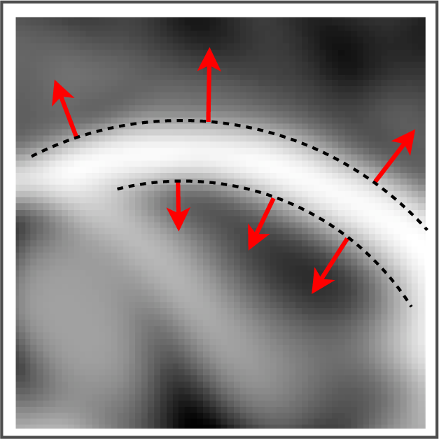
Images can be registered using either the L²-difference defined in Example 1 or with other dissimilarity measures, such as mutual information or the correlation ratio [33,34]. The similarity will be invariant to any infinitesimal deformation orthogonal to the gradient of dissimilarity measure. In the L² case, this is equivalent to any infinitesimal deformation orthogonal to the level sets of the moving image [35]. The momentum field thus has the form p(t) = α(t)∇φ(t).I₀ for a smooth function α(t) on M (see Figure 6), and the registration problem can be reduced to a search over the scalar field α(t) instead of vector field p(t).

Minimizers for E follow the PDE [5]:

$${\dot{u}}_t{\displaystyle {\int }_{M}K(\cdot -y)}\alpha (y)\nabla m_t(y)dy,{\dot{m}}_t=-\nabla m_t^T{u}_t,\dot{\alpha }=-\nabla \cdot (\alpha u_t)$$

(12)

with m_t representing the deformed image at time t.

In particular, the isotropy group of a source image f₀ ∈ C^∞ (M) is the subgroup of diffeomorphisms, which preserve the level sets of f₀. The quotient space Diff(M)=Iso(f₀) can be identified with the orbit of f₀ by diffeomorphisms, i.e., Diff(M)=Iso(f₀) ≅ Orb(f₀):= {φ_*f₀ | φ ∈ Diff(M)}. This orbit is difficult to identify with a more concrete object, in contrast to, e.g., the case of landmark matching. However, it can be characterized by various properties. For example, for a function f ∈ Orb(f₀) and any c ∈ f₀ (M) ⊂ ℝ, the level sets f⁻¹(c) and f₀⁻¹(c) have the same topology.

5.4. Jet Matching

In [14,36], an extension of the landmark case has been developed where higher-order spatial information is advected with the landmarks. The spaces of jet-particles arise as extensions of the reduced landmark space Q by quotienting out smaller isotropy subgroups known as jet-groups. A thorough account of jet-groups, including Lie group and algebra structures, can be found in [37] (Chapter 4). We provide a brief introduction here. Let G⁽⁰⁾ be the isotropy subgroup for a single landmark:

$$G^{(0)}:=\{\psi \in G|\psi (q)=q\}$$

Let now k be a positive integer. For any k-differentiable map f from a neighbourhood of q, the k-jet of f is denoted ${\mathrm{J}}_q^{(k)}(f)$. In coordinates, ${\mathrm{J}}_q^{(k)}(f)$consists of the coefficients of the k-th order Taylor expansions of f aboutx. The higher-order isotropy subgroups are then given by:

$$G^{(k)}:=\{\psi \in G^{(0)}|{\mathrm{J}}_q^{(k)}\psi ={\mathrm{J}}_q^{(k)}id\}$$

That is, the elements of G^(k) fix the Taylor expansion of the deformation φ up to order k. The definition naturally extends to finite numbers of landmarks, and the quotients Q^(k) = G/G^(k) can be identified as the sets:

$$\begin{array}{l}{Q}^{(0)}=\{(q_1,\dots ,q_N)|q_i\in M\}\\ Q^{(1)}=\{((q_i^{(0)},q_i^{(1)}),\dots )|(q_i^{(0)},q_i^{(1)},\dots )\in M\times \mathrm{GL}(d)\}\\ Q^{(2)}=\{((q_i^{(0)},q_i^{(1)},q_i^{(2)}),\dots )|q_i^{(0)},q_i^{(1)},q_i^{(2)},\dots )\in M\times \mathrm{GL}(d)\times S_2^1\}\end{array}$$

with $S_2^1$being the space of rank (1, 2) tensors symmetric in the lower indices. Intuitively, the space Q⁽⁰⁾ is the regular landmark space with information about the position of the points; the one-jet space Q⁽¹⁾ carries for each jet information about the position and the Jacobian matrix of the warp at the jet position; and the two-jet space Q⁽²⁾ carries in addition the Hessian matrix of the warp at the jet position. The momentum for Q⁽⁰⁾ in coordinates consists of N vectors representing the local displacement of the points. With the one-jet space Q⁽⁰⁾, the momentum in addition contains d × d matrices that can be interpreted as locally linear deformations at the jet positions [36]. In combination with the displacement, the one-jet momenta can thus be regarded as locally affine transformations. The momentum fields for Q⁽²⁾ add symmetric tensors encoding local second order deformation. The local effect of the jet-particles is sketched in Figure 7.

When the dissimilarity measure F is dependent not just on positions, but also on higher-order information around the points, reduction by symmetry implies that optimal solutions for E will be parametrized by k-jets in the same way as Q⁽⁰⁾ parametrizesoptimal paths for E in the landmark case. The higher-order jets can thus be used for landmark matching when the dissimilarity measure is dependent on the local geometry around the landmarks. For example, matching of the first order structure, such as image gradients, leads to first-order jets, and matching of local curvature leads to second-order jets.

5.5. Discrete Image Matching

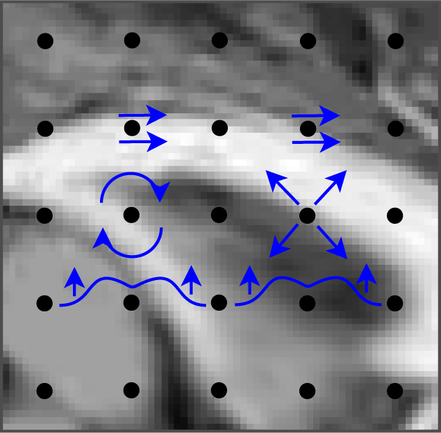
The image matching problem can be discretized by evaluating the L²-difference at a finite number of points. In practice, this always happens when the integral ${\displaystyle {\int }_M|I_0\circ {\phi }^{-1}(x)-I_1(x){|}^{2}dx}$is evaluated at finitely many pixels of the image. In [36,38], it is shown how this reduces the image matching PDE (12) to a finite dimensional system on Q when the integral is approximated by pointwise evaluation at a grid Λ_h:

$$F^{(0)}(\phi )\approx {\displaystyle \sum _{x\in {\Lambda }_h}{h}^d|I_0({\phi }^{-1}(x)-I_1(x)}{|}^2$$

(13)

where h > 0 denotes the grid spacing. F⁽⁰⁾ approximates F to order O(h^d), d = dim(M). The reduced space Q encodes the position of the points φ⁻¹(x), x ∈ Λ_h, and the lifted Eulerian momentum field is a finite sum of point measures $p={\displaystyle {\sum }_{x\in {\Lambda }_h}{a}_x\otimes {\delta }_{{\phi }^{-1}(x)}}$. For each grid point, the momentum encodes the local displacement of the point.

In [38], a discretization scheme with higher-order accuracy is in addition introduced with an O(h^d+2) approximation F⁽²⁾ of F. The increased accuracy results in the entire energy E being approximated to order O(h^d+2). The solution space in these cases becomes the jet-space Q⁽²⁾. For a given order of approximation, a corresponding reduction in the number of required discretization points is obtained. The reduction is countered by the increased information encoded in each two-jet. The momentum field thus encodes both local displacement, local linear deformation and second order deformation; see Figure 7. The discrete solutions will converge to solutions of the non-discretized problem as h → 0.

5.6. DWI/DTI Matching

Image matching is invariant with respect to variations parallel to the level lines of the images. With diffusion weighted images (DWI) and the variety of models for the diffusion information (e.g., diffusion tensor imaging (DTI) [39], Gaussian mixture fields [40]), first or higher-order information can be reintroduced into the matching problem. In essence, by letting the dissimilarity measure depend on the diffusion information, the isotropy subgroup of the matching problem becomes smaller.

The exact form of the of DWI matching problem depends on the diffusion model and how Diff(M) acts on the diffusion image. In [41], the diffusion is represented by the principal direction of the diffusion tensor, and the data objects to be matched are thus vector fields. The action by elements of Diff(M) is defined by:

$$\phi \cdot I(x)=\frac{\Vert I\circ {\phi }^{-1}\Vert }{\Vert D\phi I\circ {\phi }^{-1}\Vert }D\phi I\circ {\phi }^{-1}.$$

The action rotates the diffusion vector by the Jacobian of the warp, keeping its length fixed. Similar models can be applied to DTI with the preservation of principle direction scheme (PPD, [42,43]) and to GMF-based models [44]. The dependency on the Jacobian matrix implies that a reduced model must carry first order information in a similar fashion to the one-jet space Q⁽¹⁾; however, any irrotational part of the Jacobian can be removed by symmetry. The full effect of this has yet to be explored.

As in the case of image matching, the quotient can be identified with the orbit of the source data under diffeomorphisms.

5.7. Fluid Mechanics

Incidentally, the equation of motion:

$${\partial }_t{m}_t+{\mathrm{L}}_u[m_t]=0,u_t=K*m_t$$

is an eccentric way of writing Euler’s equation for an inviscid incompressible fluid if we assume $u_t\in \mathfrak{X}({ℝ}^n)$is initially in the space of divergence free vector-fields and K∗ is the Riemannian flat map (which implies that m_t and u_t can be identified as functions on ℝⁿ) [45]. This fact was exploited in [46] to create a sequence of regularized models to Euler’s equations by considering a sequence of kernels, such that the operator K∗ (viewed as a map to one-form densities) converges to a surjection onto the annihilator gradient vector-fields (this is written as a projection onto divergence free vector-fields in [46]). Moreover, if one replaces Diff(M) by the subgroup of volume preserving diffeomorphisms Diff_vol(M), then (formally) one can produce incompressible particle methods using the same reduction arguments presented here. In fact, jet-particles were independently discovered in this context as a means of simulating fluids in [47]. It is notable that [47] is a mechanics paper, and the particle methods that were produced were approached from the perspective of reduction by symmetry without any knowledge of the related work being done in image registration.

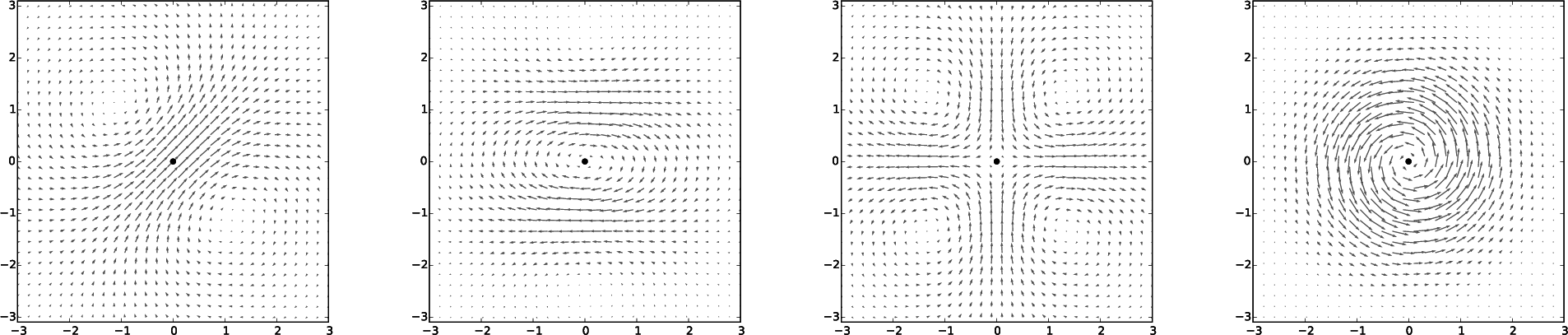
In [48], one of the kernel parameters in [46], which controls the compressibility of the u, was taken to the incompressible limit. This allowed a realization of the particle methods described in [47]. The constructions of [48] are the same as presented in this article, but with Diff(M) replaced by the group of volume-preserving diffeomorphisms of ℝ^d. Velocity fields induced by first order jet-particles are visualized in Figure 8.

6. Discussion and Conclusions

The information available for solving the registration problem is in practice not sufficient for uniquely encoding the deformation between the objects to be registered. Symmetry arises in both particle relabelling symmetry that gives the Eulerian formulation of the equations of motion and in symmetry groups for specific dissimilarity measures.

For landmark matching, reduction by symmetry reduces the infinite dimensional registration problem to a finite dimensional problem on the reduced landmark space Q. For matching curves and surfaces, symmetry implies that the momentum stays concentrated at the curves and surfaces allowing a reduction by the isotropy groups of warps that leave the objects fixed. In image matching, symmetry allows reduction by the group of warps that do not change the level sets of the image. Jet-particles arise from smaller isotropy subgroups and, hence, larger reduced spaces Q⁽¹⁾ and Q⁽²⁾ that encode locally affine and second order information.

Reduction by symmetry allows these cases to be handled in one theoretical framework. We have surveyed the mathematical construction behind the reduction approach and its relation to the above-mentioned examples. As data complexity rises both in terms of resolution and structure, symmetry will continue to be an important tool for removing redundant information and achieving compact data representations.

References

- Younes, L. Shapes and Diffeomorphisms; Springer-Berlin: Heidelberg, Germany, 2010. [Google Scholar]
- Brox, T.; Bruhn, A.; Papenberg, N.; Weickert, J. High Accuracy Optical Flow Estimation Based on a Theory for Warping. In Computer Vision-ECCV 2004; aPajdla, T., Matas, J., Eds.; Springer-Berlin: Heidelberg, Germany, 2004; pp. 25–36. [Google Scholar]
- Dawn, S.; Saxena, V.; Sharma, B. Remote Sensing Image Registration Techniques: A Survey. In Image and Signal Processing; Elmoataz, A., Lezoray, O., Nouboud, F., Mammass, D., Meunier,, J., Eds.; Springer-Berlin: Heidelberg, Germany, 2010; pp. 103–112. [Google Scholar]
- Sotiras, A.; Davatzikos, C.; Paragios, N. Deformable Medical Image Registration: A Survey. IEEE Trans. Med. Imag 2013, 32, 1153–1190. [Google Scholar]
- Younes, L.; Arrate, F.; Miller, M.I. Evolutions equations in computational anatomy. NeuroImage 2009, 45, S40–S50. [Google Scholar]
- Boyes, R.G.; Rueckert, D.; Aljabar, P.; Whitwell, J.; Schott, J.M.; Hill, D.L.G.; Fox, N.C. Cerebral atrophy measurements using Jacobian integration: Comparison with the boundary shift integral. NeuroImage 2006, 32, 159–169. [Google Scholar]
- Gorbunova, V.; Jacobs, S.S.A.M.; Lo, P.; Dirksen, A.; Nielsen, M.; Bab-Hadiashar, A.; de Bruijne, M. Early detection of emphysema progression. In Medical Image Computing and Computer-Assisted Intervention–MICCAI 2010; Springer-Berlin: Heidelberg, Germany, 2010; Volume 13, pp. 193–200. [Google Scholar]
- Joshi, S.C.; Miller, M.I.; Grenander, U. On the Geometry and Shape of Brain Sub-Manifolds. Int. J. Patt. Recogn. Artif. Intell 1997, 11, 1317–1343. [Google Scholar]
- Dupuis, P.; Grenander, U.; Miller, M.I. Variational Problems on Flows of Diffeomorphisms for Image Matching. Q. Appl. Math. 1998, 56, 587–600. [Google Scholar]
- Trouvé, A. An Infinite Dimensional Group Approach for Physics Based Models in Pattern Recognition, 1995. Available online: http://cis.jhu.edu/publications/papers_in_database/alain/trouve1995.pdf accessed on 28 April 2015.
- Christensen, G.; Rabbitt, R.; Miller, M. Deformable templates using large deformation kinematics. IEEE Trans. Image Process 1996, 5, 1435–1447. [Google Scholar]
- Holm, D.D.; Ratnanather, J.T.; Trouvé, A.; Younes, L. Soliton Dynamics in Computational Anatomy. NeuroImage 2004, 23, S170–S178. [Google Scholar]
- Bruveris, M.; Gay-Balmaz, F.; Holm, D.D.; Ratiu, T.S. The momentum map representation of images. J. Nonlinear Sci 2011, 21, 115–150. [Google Scholar]
- Jacobs, H. Symmetries in LDDMM with higher order momentum distributions, 2013, arXiv, p. 1306.3309. arXiv.org e-Print archive. Available online: http://arxiv.org/abs/1306.3309 accessed on 28 April 2015.
- Pennec, X.; Stefanescu, R.; Arsigny, V.; Fillard, P.; Ayache, N. Riemannian Elasticity: A Statistical Regularization Framework for Non-linear Registration. In MICCAI 2005; Springer-Berlin: Heidelberg, Germany, 2005; pp. 943–950. [Google Scholar]
- Derfoul, R.; Le Guyader, C. A. Relaxed Problem of Registration Based on the Saint Venant–Kirchhoff Material Stored Energy for the Mapping of Mouse Brain Gene Expression Data to a Neuroanatomical Mouse Atlas. SIAM J. Imag. Sci. 2014, 7, 2175–2195. [Google Scholar]
- Rueckert, D.; Sonoda, L.I.; Hayes, C.; Hill, D.L.; Leach, M.O.; Hawkes, D.J. Nonrigid registration using free-form deformations: Application to breast MR images. IEEE Trans. Med. Imag. 1999, 18, 712–721. [Google Scholar]
- Horn, B.K.; Schunck, B.G. Determining optical flow. Artif. Intell. 1981, 17, 185–203. [Google Scholar]
- Trouvé, A.; Younes, L. Local geometry of deformable templates. SIAM J. Math. Anal. 2005, 37, 17–59. [Google Scholar]
- Abraham, R.; Marsden, J.E. Foundations of Mechanics; Benjamin/Cummings Publishing Co. Inc.: Reading, MA, USA, 1978. [Google Scholar]
- Kobayashi, S.; Nomizu, K. Foundations of Differential Geometry, Volume I; Wiley Classics Library, John Wiley & Sons, Inc: New York, NY, USA, 1996. [Google Scholar]
- Taylor, M. Pseudo Differential Operators; Springer-Verlag: Berlin, Germany; New York, NY, USA, 1974. [Google Scholar]
- Holm, D.D.; Marsden, J.E. Momentum maps and measure-valued solutions (peakons, filaments, and sheets) for the EPDiff equation. In The Breadth of Symplectic and Poisson Geometry; Birkhäuser Boston: Boston, MA, USA, 2005; Volume 232, pp. 203–235. [Google Scholar]
- Micheli, M.; Glaunès, J.A. Matrix-valued Kernels for Shape Deformation Analysis. Geometry Imag. Comput 2014, 1, 57–39. [Google Scholar]
- Dupuis, P.; Grenander, U.; Miller, M.I. Variational problems on flows of diffeomorphisms for image matching. Quart. Appl. Math. 1998, 56, 587–600. [Google Scholar]
- Beg, M.F.; Miller, M.I.; Trouvé, A.; Younes, L. Computing Large Deformation Metric Mappings via Geodesic Flows of Diffeomorphisms. IJCV 2005, 61, 139–157. [Google Scholar]
- Joshi, S.; Miller, M. Landmark matching via large deformation diffeomorphisms. IEEE Trans. Image Process 2000, 9, 1357–1370. [Google Scholar]
- Vaillant, M.; Miller, M.; Younes, L.; Trouvé, A. Statistics on diffeomorphisms via tangent space representations. NeuroImage 2004, 23, S161–S169. [Google Scholar]
- Gay-Balmaz, F.; Vizman, C. Dual pairs in fluid dynamics. Ann. Glob. Anal. Geometry. 2012, 41, 1–24. [Google Scholar]
- Bauer, M.; Bruveris, M.; Michor, P.W. Overview of the Geometries of Shape Spaces and Diffeomorphism Groups. J. Math. Imag. Vis. 2014, 50, 60–97. [Google Scholar]
- Vaillant, M.; Glaunès, J. Surface Matching via Currents. In Information Processing in Medical Imaging; Springer-Berlin: Heidelberg, Germany, 2010; pp. 381–392. [Google Scholar]
- Glaunès, J. Transport Par Difféomorphismes de Points, de Mesures et de Courants Pour La Comparaison de Formes et L’anatomie Numérique. Ph.D. Thesis, Université Paris 13, Villetaneuse, France, 2005. [Google Scholar]
- Wells, W.M., III; Viola,, P.; Kikinis,, R. Multi-Modal Volume Registration by Maximization of Mutual Information. Med. Image Anal 1996, 1, 35–51. [Google Scholar]
- Roche, A.; Malandain, G.; Pennec, X.; Ayache, N. The Correlation Ratio as a New Similarity Measure for Multimodal Image Registration. In Proceedings of the First International Conference on Medical Image Computing and Computer-Assisted Intervention. In MICCAI 1998; Springer-Berlin: Heidelberg, Germany, 1998; pp. 1115–1124, ACM ID: 709612. [Google Scholar]
- Miller, M.I.; Trouvé, A.; Younes, L. Geodesic Shooting for Computational Anatomy. J. Math. Imag. Vis. 2006, 24, 209–228. [Google Scholar]
- Sommer, S.; Nielsen, M.; Darkner, S.; Pennec, X. Higher-Order Momentum Distributions and Locally Affine LDDMM Registration. SIAM J. Imag. Sci. 2013, 6, 341–367. [Google Scholar]
- Kolář, I.; Michor, P.W.; Slovák, J. Natural Operations in Differential Geometry; Springer Verlag: Berlin, Germany, 1999. [Google Scholar]
- Jacobs, H.O.; Sommer, S. Higher-order Spatial Accuracy in Diffeomorphic Image Registration. J. Geom. Imaging Comput, 2015. in press. Available online: http://arxiv.org/abs/1412.7504 accessed on 28 April 2015. [Google Scholar]
- Basser, P.J.; Mattiello, J.; LeBihan, D. Estimation of the effective self-diffusion tensor from the NMR spin echo. J. Magn. Resonance Ser. B 1994, 103, 247–254. [Google Scholar]
- Jian, B.; Vemuri, B.C.A. Unified Computational Framework for Deconvolution to Reconstruct Multiple Fibers From Diffusion Weighted MRI. IEEE Trans. Med. Imag 2007, 26, 1464–1471. [Google Scholar]
- Cao, Y.; Miller, M.I.; Winslow, R.L.; Younes, L. Large deformation diffeomorphic metric mapping of vector fields. IEEE Trans. Med. Imag. 2005, 24, 1216–1230. [Google Scholar]
- Alexander, D.C.; Gee, J.C.; Bajcsy, R. Strategies for Data Reorientation during Non-rigid Warps of Diffusion Tensor Images. In Medical Image Computing and Computer-Assisted Intervention—MICCAI’99; Taylor, C., Colchester, A., Eds.; Number 1679 in Lecture Notes in Computer Science; Springer-Verlag: Berlin, Germany, 1999; pp. 463–472. [Google Scholar]
- Alexander, D.C.; Pierpaoli, C.; Basser, P.J.; Gee, J.C. Spatial transformations of diffusion tensor magnetic resonance images. IEEE Trans. Med. Imag. 2001, 20, 1131–1139. [Google Scholar]
- Cheng, G.; Vemuri, B.C.; Carney, P.R.; Mareci, T.H. Non-rigid Registration of High Angular Resolution Diffusion Images Represented by Gaussian Mixture Fields. In Medical Image Computing and Computer-Assisted Intervention—MICCAI 2009; Springer-Verlag: Berlin, Germany, 2009; pp. 190–197. [Google Scholar]
- Arnold, V.I. Sur la géométrie différentielle des groupes de Lie de dimension infinie et ses applications à l’hydrodynamique des fluides parfaits. Ann. l’Instit. Fourier 1966, 16, 316–361. [Google Scholar]
- Mumford, D.; Michor, P.W. On Euler’s equation and “EPDiff”. J. Geometr. Mech 2013, 5, 319–344. [Google Scholar]
- Jacobs, H.O.; Ratiu, T.S.; Desbrun, M. On the coupling between an ideal fluid and immersed particles. Phys. D Nonlinear Phenome 2013, 265, 40–56. [Google Scholar]
- Cotter, C.J.; Holm, D.D.; Jacobs, H.O.; Meier, D.M. A jetlet hierarchy for ideal fluid dynamics. J. Phys. A Math. Theor. 2014, 47, 352001. [Google Scholar]