Multilevel Editing of B-Spline Curves with Robust Orientation of Details

Abstract

We facilitate the editing of hierarchical B-spline curves at multiple resolutions by expressing a displacement function at each level in rotation minimizing frames (RMFs) on the curve at the next lower level. When the curve is edited at a particular level, RMFs at all the higher levels are updated, and the control points of the displacement function at each higher level are obtained from these new RMFs. This transfers details created at the current level to higher levels. Our method presents a hundred-fold faster way to reflect editing results compared to the traditional approach using Frenet frames. We demonstrate the effectiveness of our technique by showing several examples of editing curves with fine details.

1. Introduction

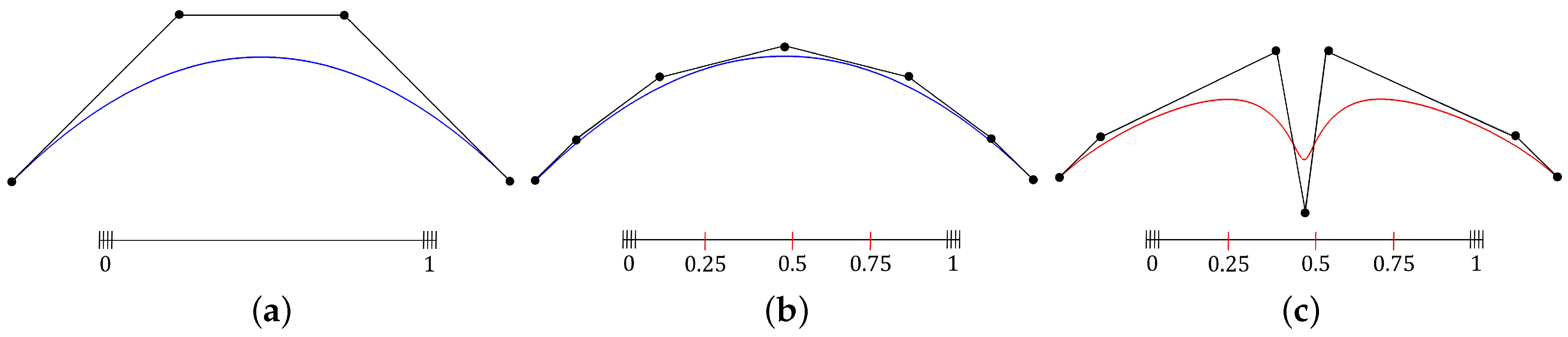
Thanks to useful properties of B-spline, it has been considered the de factor standard for modeling freeform curves and surfaces in computer-aided design and computer graphics [1,2]. Knot insertion property provides an additional degree of freedom for refining B-spline curves and surfaces without any change in their shape. Figure 1 shows an example of designing a B-spline curve using knot insertion technique.

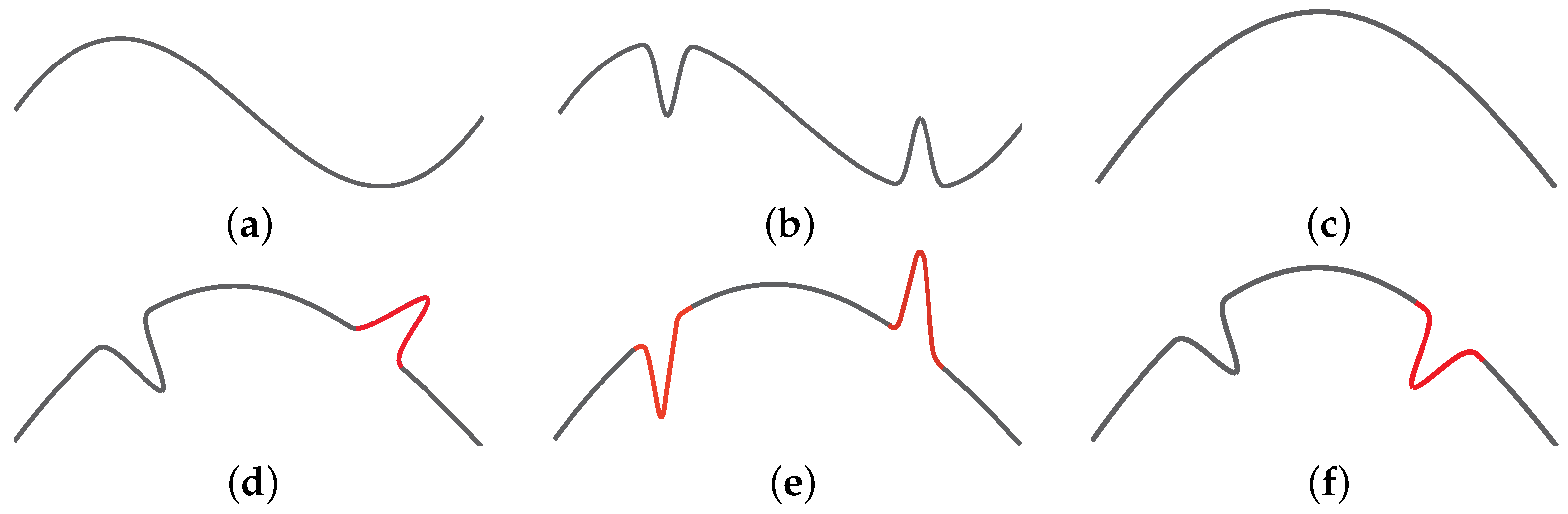
Hierarchical B-splines [3] support the editing of curves and surfaces at multiple levels of detail using knot insertion or refinement. Figure 2 illustrates typical multilevel editing processes. Figure 2a shows a cubic B-spline curve represented at a low level (i.e., with few knots) and Figure 2b shows the result of editing the same curve at a higher level (i.e., after extra knots have been inserted). If a user goes back to the lower level, edits the curve in the way shown in Figure 2c, and then returns to the higher level, we would expect the curve to have the shape shown in Figure 2d. However, the actual result is the same as Figure 2e because the edited displacements at the higher level are represented in a fixed coordinate system. If we expect to maintain the orientation of the details made at the higher level, the edited displacements should be represented in certain coordinate frames on the curve at the lower level.

One obvious choice for the local coordinate systems can be the Frenet frames. Finkelstein and Salesin [4] discussed the orientation of details in this type of editing. They used the Frenet frames (i.e., tangent, normal and bi-normal to a curve) to define a local coordinate system. However, the normal vectors are obtained from the second derivatives of a curve, and thus they can suddenly flip at inflection points while generating undesired effects. Figure 2f illustrates this problem in which the edited displacements are added to a curve in the opposite direction.

In this paper, we extend the traditional method for multilevel editing of B-spline curves to have correct orientation of details at each editing level. For this, we employ the rotation minimizing frames (RMFs) [5] of a curve as the reference coordinate system. RMFs are obtained from only tangent vectors in a way that minimizes the rotation between successive frames. Tangent vectors are the first derivatives of a curve, and thus they do not suffer from the flipping problems caused by the Frenet frames. The use of RMFs guarantees stable local frames regardless of the shape or degree of a curve. Displacements introduced at a level j are represented in RMFs at a level $j-1$, and thus changes made at higher levels are accurately retained, as shown in Figure 2d.

Our multilevel editing technique can effectively be used for modeling planar or spatial B-spline curves with highly detailed shapes. A user can easily change the overall shape of a curve, while preserving the orientation of details edited at higher levels. We also apply our technique to the multilevel editing of camera motions, which can easily be achieved by editing the associated curve component.

The main contributions of this work can be summarized as follows:

• We present a robust and effective method for preserving orientation of details in the multilevel editing of B-spline curves.
• We choose RMFs as the reference coordinate system and show that they are stable and suitable for preserving orientation of details rather compared to other reference frames.
• Our technique can easily be applied to the multilevel editing of 3D camera motions by editing its curve component.

The rest of this paper is organized as follow. In Section 2 we briefly summarize related recent work on multilevel editing of B-spline curves and surfaces. Section 3 defines a multilevel B-spline curve with orientation of details. In Section 4, the multilevel editing of B-spline curves is explained in details, and experimental results are then presented in Section 5. Finally, we conclude this paper in Section 6 and suggest future work.

2. Related Work

Forsey and Bartel [3] introduced a hierarchical B-spline representation which uses a knot refinement and overlay technique. This representation allows a user to edit a B-spline surface at different levels of detail by specifying offset displacements which are represented relatively to a local frame. For regular surfaces, a tangent plane can provide the reference coordinate system. However, it is difficult for curves to choose reference coordinate frames which are defined smoothly over the entire curve. Finkelstein and Salesin [4] proposed a multiresolution representation of a curve using wavelets that allows the curve to be edited while its details are preserved. However, the reference frames required for local editing are not stable since they can flip at inflection points of a curve. Recently, hierarchical B-splines have been widely used not only in geometry modeling but also geometry analysis. Vuong et al. [6] employed hierarchical B-splines for local refinement in isogeometry analysis and Bornemann and Cirak [7] presented a subdivision scheme for easy implementation of hierarchical B-splines and succeeded to integrate them into existing finite element software.

Elber and Gotsman [8] extended the multiresolution representation of uniform B-spline curves to non-uniform rational B-splines, and presented a technique for converting NURBS curves to their multiresolution representation, with an error that is minimized. Prusinkiewicz et al. [9] and Poon et al. [10] presented a multiresolution representation in which a curve is subdivided by means of an L-system. Dreger et al. [11] proposed a multiresolution representation of triangular B-spline surfaces of arbitrary degree.

Recently, a variety of multiresolution editing techniques satisfying given geometric constraints have been proposed. Elber [12] introduced a multiresolution editing technique that satisfies a symmetric linear constraint. Hahmann et al. [13] proposed a multiresolution editing technique for preserving the area of a closed planar curves, while Sauvage et al. [14] preserved the length of a curve. Olsen et al. [15] showed how to construct a multiresolution local filter for B-splines based on subdivision curves. This technique can be applied efficiently to the subdivision of meshes with arbitrary topologies. Li el al. [16] constructed multiresolution curves using constrained B-spline wavelets. For polygonal meshes, Kobbelt and Botsch [17] proposed a new multiresolution model based on volume elements. The details between different levels are encoded by displacement volumes and they are added to the base surface without self-intersections when the base surface is edited. However, none of these methods except our previous work [18] deal with the problem of preserving the orientation of details.

In this paper, we deal with the orientation of details in multilevel editing of B-spline curves. For this end, we need a reference coordinate system in which the edited details can be represented robustly. A moving frame that does not rotate about the instantaneous tangent of a curve is called a rotation minimizing frame (RMF). RMFs are widely used in many applications in computer graphics, sweep surface modeling [19], generalized cylinder modeling [20,21] and motion design and control [22]. However, exact RMF (i.e., closed form) computation is non-trivial and thus a number of approximation techniques [5,23,24,25] have been proposed. We employ RMFs as a reference coordinate system and represent the edited details in RMFs.

3. Multilevel Representation of B-Spline Curves

3.1. Multilevel B-Spline Curves

A B-spline curve of degree p is defined as follows:

$$\begin{array}{c}\hfill C^0(u)=\sum _{i=0}^n{\mathbf{p}}_i{N}_i^p(u)u_p\le u\le u_{m-p}\end{array}$$

(1)

where $\{{\mathbf{p}}_i\}$ are control points and $N_i^p(u)$ is the i-th B-spline basis function of degree p defined on the knot vector $U^0=\{u_0,u_1,\cdots ,u_p,\cdots ,u_{m-p},\cdots ,u_m\}$.

We construct the refined knot vector $U^1$ by inserting a midpoint between consecutive knot values $u_i$ and $u_{i+1}$ $(p\le i\le m-p-1)$ in $U^0$ as follows:

$$U^1=\{u_0,u_1,\cdots ,u_p,\frac{u_p+u_{p+1}}{2},u_{p+1},\cdots ,u_{m-p-1},\frac{u_{m-p-1}+u_{m-p}}{2},u_{m-p},u_{m-p+1},\cdots ,u_m\}.$$

We can define a displacement function $D^1(u)$ on the refined knot vector $U^1$ as follows:

$$\begin{array}{ccc}\hfill D^1(u)& =& \sum _{i=0}^{|U^1|-1}{\mathbf{d}}_i^1{N}_i^p(u)\hfill \end{array}$$

(2)

where $|U^1|$ is the number of B-spline basis functions defined on the refined knot vector $U^1$, and $\{{\mathbf{d}}_i^1\}$ are control points, all initialized to $\overrightarrow{0}$. We construct various levels of displacement functions $D^j(u),j=1,2,\cdots ,k$ by repeating this midpoint refinement process and obtain a multilevel B-spline curve $C^k(u)$ with level $k(>0)$ as follows:

$$\begin{array}{ccc}\hfill C^k(u)& =& C^0(u)+D^1(u)+D^2(u)+\cdots +D^k(u)=C^0(u)+\sum _{j=1}^k{D}^j(u)\hfill \end{array}$$

(3)

We can edit the B-spline curve $C^k(u)$ at any level $j(0\le j\le k)$ by editing the corresponding displacement function $D^j(u)$ or $C^0(u)$. At lower levels, this displacement function affects a large region of the curve, but at higher levels it has a much more local effect. This allows us to create fine details on the curve, which will be preserved during subsequent global changes.

3.2. Multilevel B-Spline Curves with Orientation of Details

In general, the control points ${\mathbf{d}}_i^j$ of the displacement function $D^j(u)$ are represented in a fixed coordinate system, producing the undesired results shown in Figure 2e, that we have already discussed. To obtain the expected results, the displacement function $D^j(u)$ must be represented in appropriate coordinate systems defined on the curve $C^{j-1}(u)$. In this paper, we extend the definition of a multilevel B-spline curve in Equation (3) so that it can include the orientation of details as follows:

$$\begin{array}{ccc}\hfill C^k(u)& =& C^0(u)+F^0(u)D^1(u)+F^1(u)D^2(u)+\cdots +F^{k-1}(u)D^k(u)\hfill \end{array}$$

(4)

where $F^{j-1}(u)$ is a one-parameter family of rotational matrices in $SO(3)$, describing the orientation of $D^j(u)$ and will be referred to as reference frames for $D^j(u)$ for $j=1,2,\cdots ,k$. There might exist several candidates for reference frames. For example, Frenet frames can be chosen for this purpose, but they depend on the second derivatives of a curve, making the Frenet frames undefined at inflection points, as shown in Figure 3b. Moreover, computing the Frenet frames is computationally inefficient since it involves the computations of second derivatives of a curve. Therefore, the reference frames are required to satisfy the following conditions:

• $F^{j-1}(u)$ should smoothly change on $C^{j-1}(u)$.
• $F^{j-1}(u)$ should minimize its variations when $C^{j-1}(u)$ is edited.
• $F^{j-1}(u)$ should be computed efficiently.

We choose rotation minimizing frames (RMFs) [5,23,24,25] for the requirement above. However, finding the explicit form of exact RMFs on general B-spline curves is known to be a non-trivial problem and thus many approximation techniques have been proposed in practice. Among these techniques, we employ the double reflection method [5] for both accuracy and efficiency. If we are given n sample points ${\mathbf{p}}_i$ and their tangent vectors ${\mathbf{t}}_i$ on a curve $C(u)$, we can easily compute a sequence of rotation minimizing frames $F_i=\left[\begin{array}{ccc}{\mathbf{t}}_i& {\mathbf{s}}_i& {\mathbf{r}}_i\end{array}\right]$ at the points ${\mathbf{p}}_i$ for $i=1,2,\cdots ,n$, where ${\mathbf{s}}_i$ and ${\mathbf{r}}_i$ are determined so that the rotation between $F_i$ and $F_{i+1}$ is minimized. Figure 3c shows RMFs computed on the points ${\mathbf{p}}_i$ on a spatial curve $C(u)$, which smoothly change their orientations on a curve $C(u)$, compared to the Frenet frames flipping at an inflection point (see Figure 3b). For more details on construction of RMFs, please refer to the reference [5].

Now we explain how to represent the displacement function $D^j(u)$ in $F^{j-1}(u)$. Instead of finding the explicit form of $F^{j-1}(u)$, we simply represent the control points ${\mathbf{d}}_i^j$ of $D^j(u)$ in the RMFs sampled from $C^{j-1}(u)$ as follows:

$$F^{j-1}({\widehat{u}}_i)=\left[\begin{array}{ccc}{\mathbf{t}}_i({\widehat{u}}_i)& {\mathbf{s}}_i({\widehat{u}}_i)& {\mathbf{r}}_i({\widehat{u}}_i)\end{array}\right]\mathrm{for}i=0,1,\cdots ,|U^j|-1$$

(5)

where $\{{\widehat{u}}_i\}$ are the node parameters specially chosen from the knot vector $U^j$ of $D^j(u)$. Even though this is an approximation to $F^{j-1}(u)D^j(u)$, it could be a practical technique for presenting the orientation of the displacement function $D^j(u)$ in RMFs on $C^{j-1}(u)$. Our multilevel B-spline curve with orientation of details can then be represented as follows:

$$\begin{array}{ccc}\hfill C^k(u)& =& C^0(u)+{\widehat{D}}^1(u)+{\widehat{D}}^2(u)+\cdots +{\widehat{D}}^k(u)\hfill \end{array}$$

(6)

where ${\widehat{D}}^j(u)={\sum }_{i=0}^{|U^j|-1}\left(F^{j-1}({\widehat{u}}_i){\mathbf{d}}_i^j\right)N_i^p(u)\mathrm{for}j=1,2,\cdots ,k$. Finally, the node parameters ${\widehat{u}}_i$ in Equation (5) are chosen at which the B-spline basis function $N_i^p(u)$ associated with the control point ${\mathbf{d}}_i^j$ has the maximum. The reason that we take such node parameters is that the corresponding $F^{j-1}({\widehat{u}}_i)$ has maximum influence on ${\mathbf{d}}_i^j$. Figure 4 shows an example of determining the node parameter for a cubic B-spline basis function $N_i^3(u)$. Figure 4a,b show the basis function $N_i^3(u)$ and its derivative $d(N_i^3(u))/du$ constructed on a non-uniform knot vector. The node parameter ${\widehat{u}}_i$ can be computed by finding the root of the following equation:

$$\begin{array}{c}\hfill \frac{d(N_i^3(u))}{du}=0.\end{array}$$

(7)

4. Multilevel Editing with Orientation of Details

For an intuitive curve editing, our system supports a direct manipulation of curve points [1]. For example, a user can select an arbitrary point $\mathbf{p}$ on $C^j(u)$ and move it to a new position ${\mathbf{p}}^{\prime }$, which produces the edited displacement $\Delta \mathbf{p}={\mathbf{p}}^{\prime }-\mathbf{p}$. Depending on the editing level j, the displacement $\Delta \mathbf{p}$ can be interpreted as the corresponding changes $\Delta {\mathbf{d}}_i^j$ in the control points ${\mathbf{d}}_i^j$ of the displacement function $D^j(u)$. Note that $\Delta {\mathbf{d}}_i^j$ is computed in the fixed coordinate system and thus must be expressed in the RMF $F^{j-1}({\widehat{u}}_i)$. This process updates the control points as follows:

$$\begin{array}{c}\hfill {\mathbf{d}}_i^j={\mathbf{d}}_i^j+{\left(F^{j-1}({\widehat{u}}_i)\right)}^{-1}\Delta {\mathbf{d}}_i^j\end{array}$$

(8)

where the inverse matrix ${\left(F^{j-1}({\widehat{u}}_i)\right)}^{-1}$ can be replaced with the transpose matrix ${\left(F^{j-1}({\widehat{u}}_i)\right)}^T$ since $F^{j-1}({\widehat{u}}_i)$ is an orthogonal matrix.

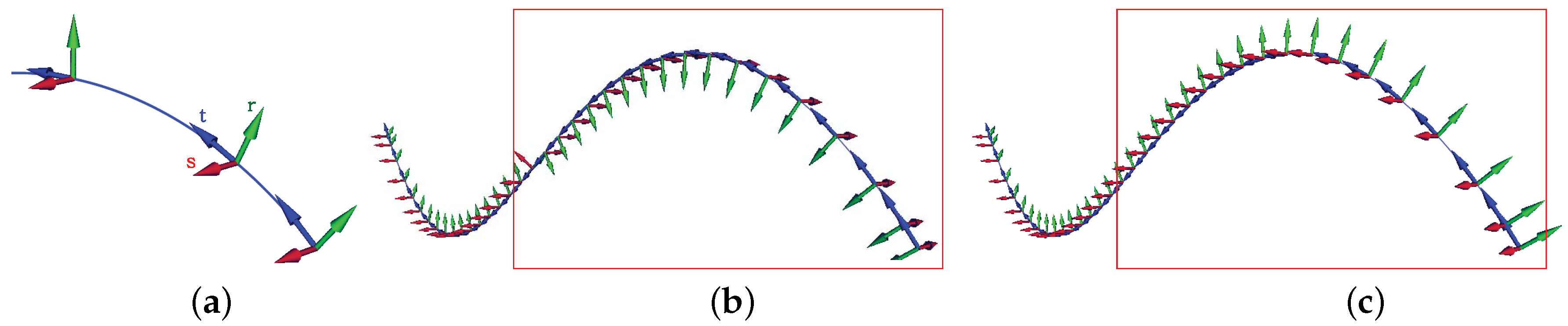
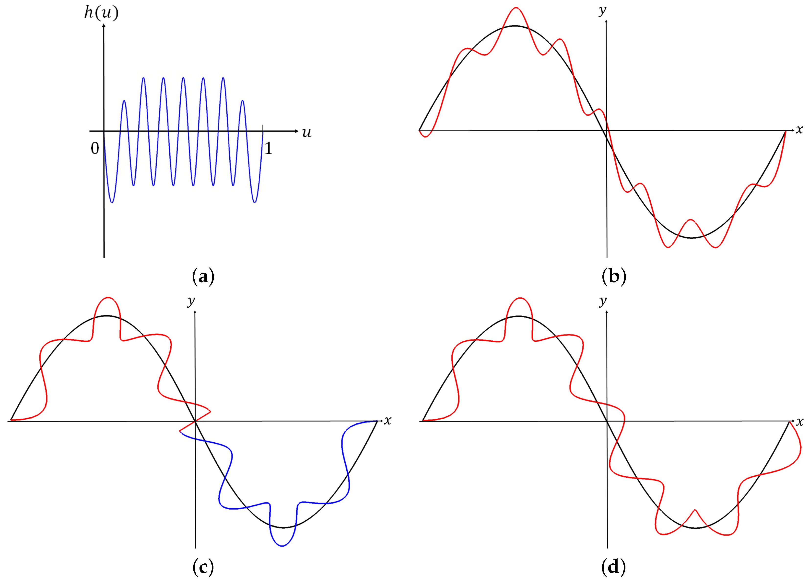
Figure 5 illustrates examples of editing a B-spline curve with and without orientation of details. Let $D^1(u)=(0,h(u),0)$ be a displacement function to be added to a curve $C^0(u)$. Figure 5a shows the graph of $h(u)$, for $u\in [0,1]$. Figure 5b–d show the results when $D^1(u)$ is added to three different reference frames on $C^0(u)$ (in black), respectively. Figure 5d shows that $D^1(u)$ is added to $C^0(u)$ while keeping its orientation correctly, whereas it flips at the origin where the second derivative of $C^0(u)$ vanishes in Figure 5c.

Algorithm 1 shows the pseudo code for multilevel editing of a B-spline curve while preserving the orientation of details. Note that if the displacement function $D^j(u)$ at level j is edited, then all RMFs in the next levels from j to k should be updated (in lines 3–11 in Algorithm 1). The complexity of Algorithm 1 can be measured by counting the number of times that the lines 5 and 9 are executed. Suppose that a cubic B-spline curve $C^0(u)$ is defined on the knot vector $U^0=\{0,0,0,0,1,1,1,1\}$ and the knot vectors are repeatedly refined at midpoints as explained in Section 3. At editing level $j(>0)$, the lines 5 and 9 are executed $(3+2^j)$ times, respectively. The upper bound can be determined from ${\sum }_{j=1}^{k}2(3+2^j)$, which results in total $(6k-4+2^{k+2})$ times. Although the complexity increases exponentially, i.e., $O(2^k)$, it would be an inevitable result because the number of control points increase exponentially at each level by the midpoint refinement of knot vectors.

Algorithm 1: Multilevel editing of a B-spline curve at level j.

INPUT: j : editing level $(1\le j\le k)$ $\Delta {\mathbf{d}}_i^j$ : edited displacements of control points ${\mathbf{d}}_i^j$   OUTPUT: $C^k(u)$: curve edited at level j   1: BEGIN 2: ${\mathbf{d}}_i^j:={\mathbf{d}}_i^j+{\left(F^{j-1}({\widehat{u}}_i)\right)}^T\Delta {\mathbf{d}}_i^j;$ 3:   FOR $l=j$ TO k 4:     FOR $m=0$ TO $|U^l|-1$ 5:       ${\mathbf{d}}_m^l:=F^{l-1}({\widehat{u}}_m){\mathbf{d}}_m^l;$ 6:     END FOR 7:     $C^l(u):=C^{l-1}(u)+{\widehat{D}}^l(u);$ 8:     FOR $m=0$ TO $|U^l|-1$ 9:       Update RMFs at node parameters ${\widehat{u}}_m$ of $C^l(u);$ 10:     END FOR 11:   END FOR 12: END BEGIN   9: RETURN $C^k(u);$

5. Experimental Results

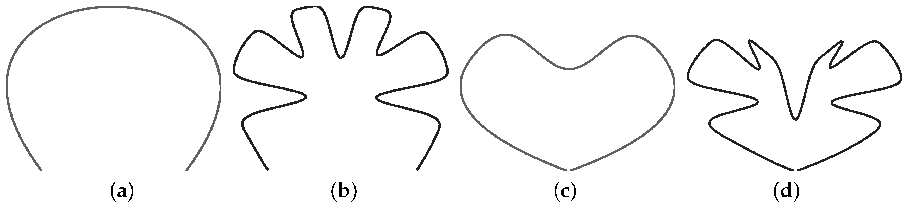
We implemented our algorithm in C++ on an Intel(R) Core(TM) i7 2.00 GHz CPU with a 16 Gb main memory and an Intel(R) Iris(TM) Pro Graphics 5200 video card. Figure 6 shows an example of multilevel editing of a B-spline curve. Figure 6a shows a cubic B-spline curve $C^0(u)$ at level 0 defined on the clamped knot vector $U^0=\{0,0,0,0,1,1,1,1\}$, and Figure 6b shows the result of editing the curve at level 5, which means the displacement function $D^5(u)$ changes. Figure 6d shows the curve at level 5 after it has been edited globally at level 0, as shown in Figure 6c. The final curve shown in Figure 6d confirms that the displacements $D^5(u)$ generated at level 5 (Figure 6b) have correctly been applied to the result of globally edited the curve at level 0.

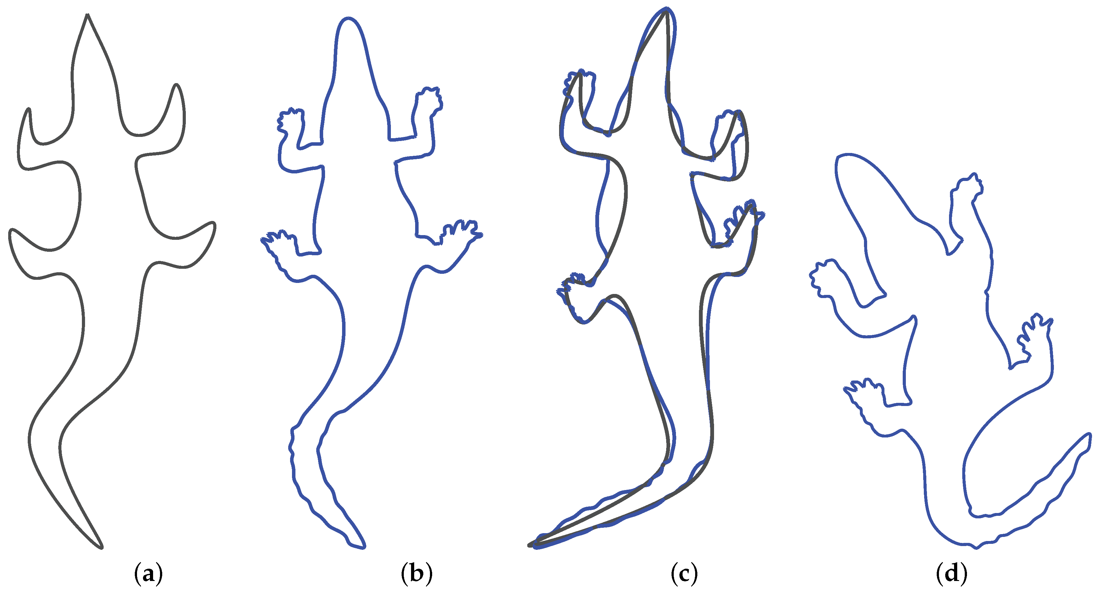
Figure 7 shows a more sophisticated example in which the initial B-spline curve (Figure 7a) is modeled by using 30 control points and it is edited at higher levels for adding fine details of a crocodile shape in Figure 7b. Figure 7c,d show the results of editing the initial curve at level 0 in which we can see that fine details made at higher levels are correctly applied to editing results at level 0.

Since the displacement function $D^j(u)$ must be applied to the curve produced at the lower level $C^{j-1}(u)$, the RMFs at the node points $C^{j-1}({\widehat{u}}_i)$ should be computed efficiently. That is, the performance of our technique depends on not only the complexity of Algorithm 1 but also the computational costs for computing references frames. In this section, we analyz the computational costs for computing a RMF and a Frenet frame at a node parameter ${\widehat{u}}_i$. For this, we assume a cubic polynomial curve $C(u)={\mathbf{p}}_0+{\mathbf{p}}_{1}u+{\mathbf{p}}_2{u}^2+{\mathbf{p}}_3{u}^3$, where ${\mathbf{p}}_i={\left[\begin{array}{ccc}{x}_i& y_i& z_i\end{array}\right]}^T\in {\mathbb{R}}^3$. The Frenet frame at a node parameter ${\widehat{u}}_i$ is computed as follows:

$$\begin{array}{c}\hfill T=\frac{C^{\prime }({\widehat{u}}_i)}{\parallel C^{\prime }({\widehat{u}}_i)\parallel },B=\frac{C^{\prime }({\widehat{u}}_i)\times C^{\prime \prime }({\widehat{u}}_i)}{\parallel C^{\prime }({\widehat{u}}_i)\times C^{\prime \prime }({\widehat{u}}_i)\parallel },N=B\times T\end{array}$$

(9)

Table 1. Operation counts to compute a RMF and a Frenet Frame.

Method	# of adds	# of mults	# of divs	# of sqrt
Frenet frame	19	42	6	2
RMF	28	32	2	0

lists the total operation counts for computing a Frenet frame and a RMF, respectively. The detailed counting for a RMF is referred to the double reflection method [5]. Note that a $sqrt$ or a division is about six times more time-consuming than a multiplication since they are approximated by a truncated series in arithmetic hardware. Table 1 just compares the operation counts for one node parameter. Multiple node parameters at higher level would produce a huge difference of the total operation counts.

Table 2. Times to compute RMFs and Frenet Frames for the curve of Figure 6.

Level	Num. of Frames	Time (ms)		Ratio (b) to (a)
		RMF (a)	Frenet (b)
1	5	0.027949	4.07133	145.6699703
2	7	0.0400458	7.48952	187.0238577
3	11	0.06561	17.68624	269.5662247
4	19	0.1188456	36.12243	303.9441931
5	35	0.211788	85.059	401.6233214

lists the actual computation times for computing RMFs and Frenet frames with a different number of reference frames at each level of the curve in Figure 6. The last column of Table 2 shows that computing RMFs are 145 to 400 times faster than Frenet frames.

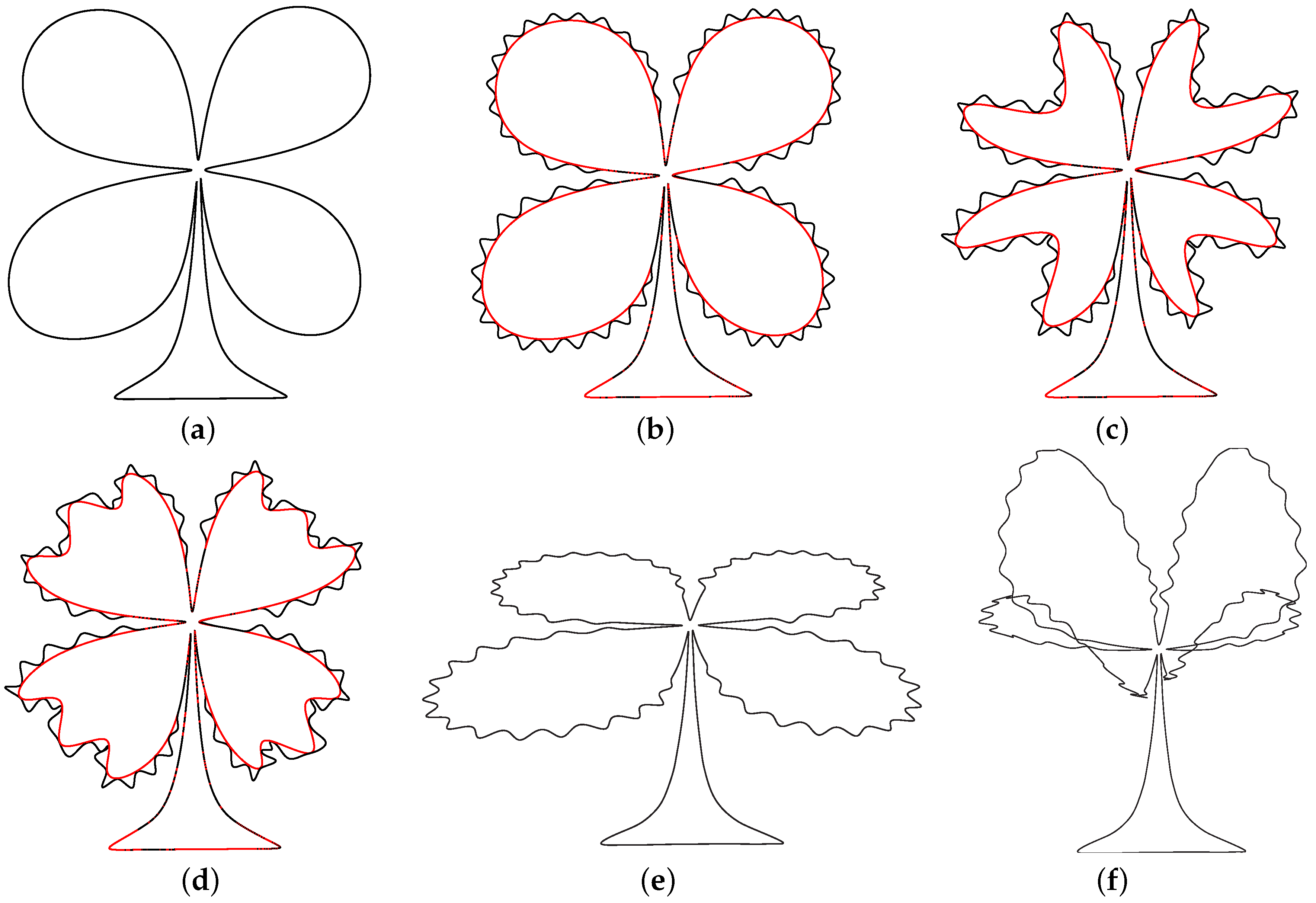
Figure 8b shows another example in which the displacement function $D^4(u)$ is applied to the curve at level 0 of Figure 8a. Figure 8c,d are curves (in black) edited at level 1 and level 2, maintaining the orientation of the displacement function $D^4(u)$. The curve can easily be edited to a spatial curve as shown in Figure 8e,f.

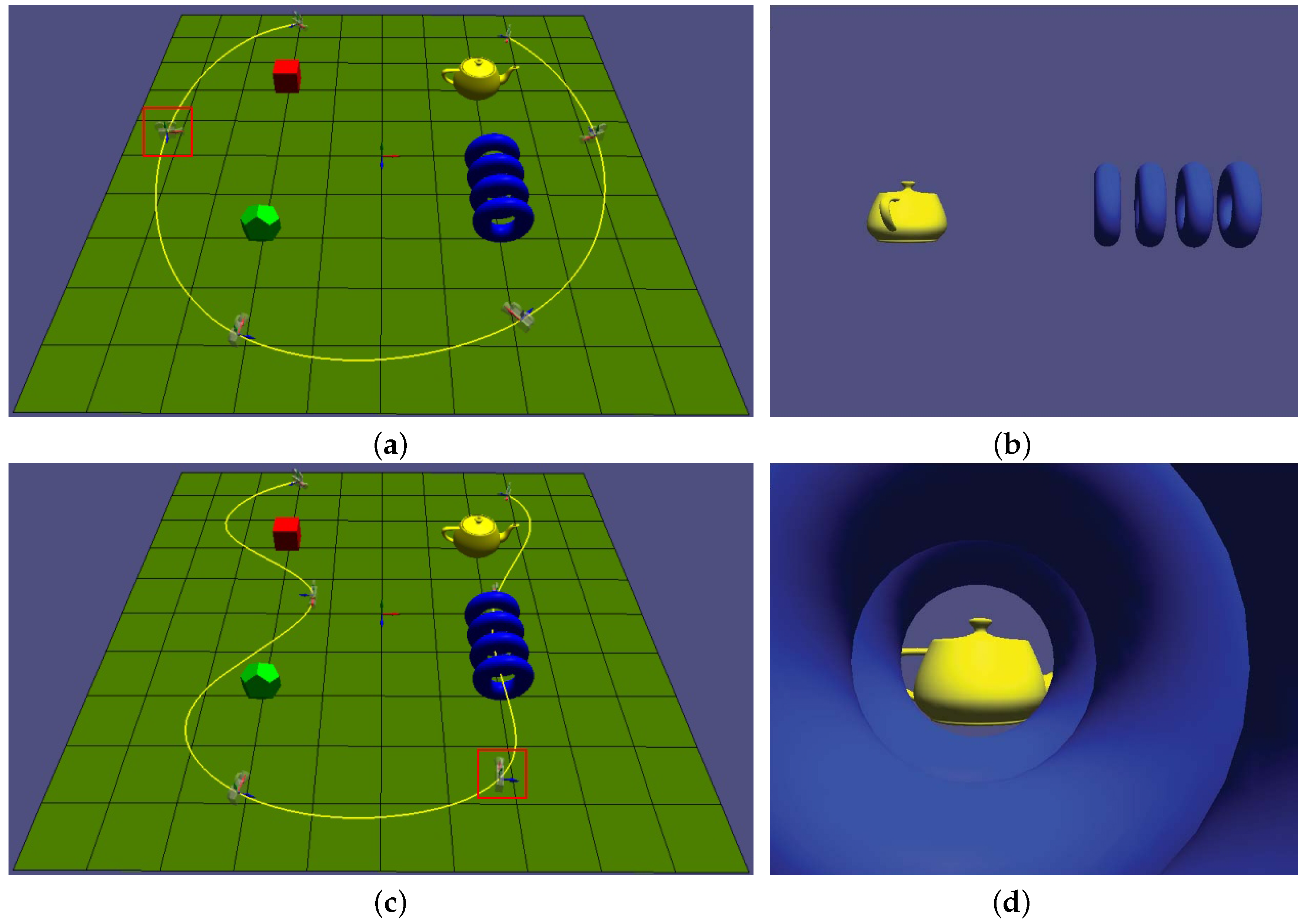
An obvious application for our multilevel curve editing technique is three-dimensional camera motion control. A camera motion is defined by a rigid-body transformation that consists of a translation and a rotation. A B-spline curve $\mathbf{t}(u)=(t_x(u),t_y(u),t_z(u))$ can be used as a trajectory for defining the position of camera at time u, and a quaternion curve $\mathbf{q}(u)=(q_w(u),q_x(u),q_y(u),q_z(u))$ can specify the orientation of the camera at time u. The translation matrix $T(u)$ is determined by a point on the trajectory curve $\mathbf{t}(u)$, and the rotation matrix $R(u)$ is determined by the orientation curve $\mathbf{q}(u)/\parallel \mathbf{q}(u)\parallel$. The rigid-body transformation of the camera $M(u)$ is then readily expressed as the product $M(u)=T(u)R(u)$. In this case, our multilevel curve editing technique enables precise modification of the trajectory and orientation curves at different levels, providing the sophisticated camera control needed for creating desired camera motion.

Figure 9a shows an example of camera control. The trajectory of the camera (shown in yellow) is a cubic B-spline curve with six control points. Figure 9b shows the image captured by the camera when it is at the position marked by the red box. Figure 9c shows detailed editing of the trajectory and orientation curves at level 2 (compare the yellow curve in Figure 9c with that of Figure 9a). The camera motion is edited so that it passes through the sequence of tori. Figure 9d shows the image captured by the camera at the position marked by the red box in Figure 9c.

Besides from 3D camera control, our technique can easily be applied to various applications making use of curve components such as modeling sweep surfaces and hierarchical editing of human motion, where trajectory curves and joint angle curves can effectively be controlled by our technique while preserving orientation of details.

6. Conclusions

We have presented a new technique for editing multilevel B-spline curves by using RMFs [5] as local reference frames. The displacement function at each level is represented in RMFs on the next lower level curve, and this preserves the orientation of local details between levels. Our method can effectively be used for editing a B-spline curve globally, while maintaining its orientation of local details. To the best of our knowledge, this is the first work to deal with the orientation of details in editing curves (except the approaches using Frenet frames). Moreover, the proposed technique is quite stable regardless of the shape or degree of a curve, and many times faster than the Frenet frames. We have demonstrated the effectiveness of our technique by showing several examples of multilevel editing B-spline curves. In future work, we plan to extend our technique to other representations such as B-spline surfaces, subdivision surfaces and implicit surfaces so that they can preserve the orientation of details and also plan to find other sophicated reference frames that can substitute for RMFs.

References

1. Piegl, L.; Tiller, W. The NURBS Book, 2nd ed.; Springer: Berlin/Heidelberg, Germany, 1997. [Google Scholar]
2. Farin, G. Curves and Surfaces for CAGD, 5th ed.; Academic Press: Cambridge, MA, USA, 2002. [Google Scholar]
3. Forsey, D.-R.; Bartels, R.-H. Hierarchical B-spline refinement. ACM SIGGRAPH Comput. Graph. 1988, 22, 205–212. [Google Scholar] [CrossRef]
4. Finkelstein, A.; Salesin, D.-H. Multiresolution curves. In Prceedings of the SIGGRAPH ‘94 21st Annual Conference on Computer Graphics and Interactive Techniques, Orlando, FL, USA, 24–29 July 1994; pp. 261–268.
5. Wang, W.; Jüttler, B.; Zheng, D.; Liu, Y. Computation of rotation minimizing frames. ACM Trans. Graph. 2008, 27, 1–18. [Google Scholar] [CrossRef]
6. Vuong, A.-V.; Giannelli, C.; Jüttler, B.; Simeon, B. A hierarchical approach to adaptive local refinement in isogeometric analysis. Comput. Methods Appl. Mech. Eng. 2011, 200, 3554–3567. [Google Scholar] [CrossRef]
7. Bornemann, P.-B.; Cirak, F. A subdivision-based implementation of the hierarchical B-spline finite element method. Comput. Methods Appl. Mech. Eng. 2013, 253, 584–598. [Google Scholar] [CrossRef]
8. Elber, G.; Gotsman, C. Multiresolution control for nonuniform B-spline curve editing. In Proceeding of the 3rd Pacific Graphics Conference on Computer Graphics and Applications, Seoul, Korea, 21–24 August 1995; pp. 267–278.
9. Prusinkiewicz, P.; Samavati, F.; Samavati, F.; Smith, C.; Karwowski, R. L-system description of subdivision curves. Int. J. Shape Model. 2002, 9, 41–59. [Google Scholar] [CrossRef]
10. Poon, K.; Bateman, L.; Karwowski, R.; Prusinkiewicz, P.; Samavati, F. L-system implementation of multiresolution curves based on cubic B-spline subdivision. In Proceedings of the 14th Western Computer Graphics Symposium, Banff, AB, Canada, 30 March–2 April 2003.
11. Dreger, A.; Gross, M.-H.; Schlegel, J. Multiresolution triangular B-spline surfaces. In Proceedings of the Computer Graphics International, Hannover, Germany, 26 June 1998; p. 166.
12. Elber, G. Multiresolution curve editing with linear constraints. In Proceedings of the 6th ACM Symposium on Solid Modeling and Applications, Ann Arbor, MI, USA, 4–8 June 2001; pp. 109–119.
13. Hahmann, S.; Sauvage, B.; Bonneau, G.-P. Area preserving deformation of multiresolution curves. Comput. Aided Geom. Des. 2005, 22, 349–367. [Google Scholar] [CrossRef]
14. Sauvage, B.; Hahmann, S.; Bonneau, G.-P. Length preserving multiresolution editing of curves. Computing 2004, 72, 161–170. [Google Scholar] [CrossRef]
15. Olsen, L.; Samavati, F.-F.; Bartels, R.-H. Multiresolution B-spline based on wavelet constraints. In Proceedings of the Eurographics Symposium on Geometric Processing, Vienna, Austria, 4–6 July 2005; pp. 1–10.
16. Li, D.; Qin, K.; Sun, H. Curve modeling with constrained B-spline wavelets. Comput. Aided Geom. Des. 2005, 22, 45–56. [Google Scholar] [CrossRef]
17. Botsch, M.; Kobbelt, L. Multiresolution surface representation based on displacement volumes. Comput. Graph. Forum 2003, 22, 483–491. [Google Scholar] [CrossRef]
18. Zhang, C.; Yoon, S.-H.; Lee, J. Multilevel Editing for Hierarchical B-spline curves using Rotation Minimizing Frames. J. Korea Comput. Graph. Soc. 2010, 16, 41–50. [Google Scholar] [CrossRef]
19. Chung, T.L.; Wang, W. Discrete moving frames for sweep surface modeling. In Proceedings of the Pacific Graphics ’96, Taipei, Taiwan, 19–22 August 1996; pp. 159–173.
20. Bloomenthal, J. Modeling the mighty maple. In Proceedings of the SIGGRAPH ’85 12th Annual Conference on Computer Graphics and Interactive Techniques, San Francisco, CA, USA, 22–26 July 1985; pp. 305–311.
21. Semwal, S. K.; Hallauer, J. Biomedical modeling: Implementing line-of-action algorithm for human muscles and bones using generalized cylinders. Comput. Graph. 1994, 18, 105–112. [Google Scholar] [CrossRef]
22. Jüttler, B. Rotational minimizing spherical motions. In Advance in Robotics; Analysis and Control; Springer: Berlin/Heidelberg, Germany, 1998; pp. 413–422. [Google Scholar]
23. Klok, F. Two moving frames for sweeping along a 3D Trajectory. Comput. Aided Geom. Des. 1986, 3, 217–229. [Google Scholar] [CrossRef]
24. Jüttler, B. Rational approximation of rotation minimizing frames using Phythagorean-hodograph cubics. J. Geom. Graph. 1999, 3, 141–159. [Google Scholar]
25. Farouki, R.T.; Giannelli, C.; Sampoli, M.L.; Sestini, A. Rotation-minimizing osculating frames. Comput. Aided Geom. Des. 2014, 31, 27–42. [Google Scholar] [CrossRef]
Figure 1. (a) A cubic B-spline curve with initial knots { 0 , 0 , 0 , 0 , 1 , 1 , 1 , 1 } ; (b) inserting three knots { 0.25 , 0.5 , 0.75 } produces additional control points without shape change; (c) a curve edited by moving additional control points.
Symmetry 08 00121 g001
Figure 2. Multilevel curve editing: (a) a cubic B-spline curve; (b) editing the curve at the higher level in a fixed coordinate system; (c) re-editing the curve at the original level; (d) the desired result after (c); (e) the real result after (c); and (f) the result using Frenet frames in (b).
Symmetry 08 00121 g002
Figure 3. Comparison of local reference frames: (a) at points on the curve; (b) based on Frenet frames; and (c) based on rotation minimizing frames (RMFs).
Symmetry 08 00121 g003
Figure 4. Determination of node parameters: (a) a cubic B-spline basis function N i 3 ( u ) and node parameter u ^ i , and (b) the derivatives of d ( N i 3 ( u ) ) / d u and u ^ i such that d ( N i 3 ( u ^ i ) ) / d u = 0 .
Symmetry 08 00121 g004
Figure 5. Adding a displacement function D 1 ( 0 , h ( u ) , 0 ) to different reference frames: (a) a graph of h ( u ) ; (b) D 1 ( u ) is added to C 0 ( u ) in a fixed coordinate system; (c) D 1 ( u ) is added to the Frenet frames on C 0 ( u ) and (d) D 1 ( u ) is added to the RMFs on C 0 ( u ) .
Symmetry 08 00121 g005
Figure 6. Results of multilevel editing: (a) initial curve at level 0; (b) the curve edited at level 5; (c) the curve edited globally at level 0; and (d) the resulting curve at level 5.
Symmetry 08 00121 g006
Figure 7. Results of multilevel editing: (a) initial curve at level 0; (b) the curve edited at higher levels; (c) and (d) the resulting curves at higher levels after the initial curve (in black) is edited at level 0.
Symmetry 08 00121 g007
Figure 8. Results of multilevel editing: (a) initial curve at level 0; (b) edited curve at level 4; (c) edited curve at level 1; (d) edited curve at level 2; (e) and (f) edited curve to be a space curve.
Symmetry 08 00121 g008
Figure 9. Camera motion control: (a) camera trajectory and orientation curves at level 0; (b) image captured by the camera at the position of the red box in (a); (c) edited camera curves at level 2; and (d) image captured by the camera at the position of the red box in (c).
Symmetry 08 00121 g009