Article

Improvement in Scoliosis Top View: Evaluation of Vertebrae Localization in Scoliotic Spine-Spine Axial Presentation

by
Paweł Główka
1,*,†,
Dominik Gaweł
2,†,
Bartosz Kasprzak
3,†,
Michał Nowak
2,† and
Tomasz Kotwicki
1,†
1
Department of Spine Disorders and Pediatric Orthopedics, University of Medical Sciences, 61-545 Poznan, Poland
2
Chair of Virtual Engineering, Poznan University of Technology, 60-965 Poznan, Poland
3
Department of Biophysics, University of Medical Sciences, 60-780 Poznan, Poland
*
Author to whom correspondence should be addressed.
These authors contributed equally to this work.
Symmetry 2016, 8(11), 125; https://doi.org/10.3390/sym8110125
Submission received: 9 August 2016 / Revised: 23 October 2016 / Accepted: 2 November 2016 / Published: 14 November 2016

Abstract

:
Morphological analysis of the scoliotic spine is based on two-dimensional X-rays: coronal and sagittal. The three-dimensional character of scoliosis has raised the necessity for analyzing scoliosis in three planes. We proposed a new user-friendly method of graphical presentation of the spine in the third plane–the Spine Axial Presentation (SAP). Eighty-five vertebrae of patients with scoliosis were analyzed. Due to different positions during X-rays (standing) and computer tomography (CT) (supine), the corresponding measurements cannot be directly compared. As a solution, a software creating Digital Reconstructed Radiographs (DRRs) from CT scans was developed to replace regular X-rays with DRRs. Based on the measurements performed on DRRs, the coordinates of vertebral bodies central points were defined. Next, the geometrical centers of vertebral bodies were determined on CT scans. The reproducibility of measurements was tested with Intraclass Correlation Coefficient (ICC), using p = 0.05. The intra-observer reproducibility and inter-observer reliability for vertebral body central point’s coordinates (x, y, z) were high for results obtained based on DRRs and CT scans, as well as for comparison results obtained based on DRR and CT scans. Based on two standard radiographs, it is possible to localize vertebral bodies in 3D space. The position of vertebral bodies can be present in the Spine Axial Presentation.

1. Introduction

The human spinal column is composed of 34 vertebrae which are set up in a specific alignment in the sagittal plane: lordosis in the cervical and lumbar parts and kyphosis in the thoracic and sacral parts. In a healthy individual in standing position one does not observe any lateral deviation of vertebrae from the midsagittal plane nor rotation of vertebrae in the axial plane. Idiopathic scoliosis is a condition where the thoracic or lumbar vertebrae are displaced in all aforementioned planes [1,2]. Treatment of spinal deformities imposes a precise description of the spatial location of each vertebra. In clinical practice, the analysis of morphology of scoliotic spine is based on two radiographic images: antero-posterior and lateral [3,4,5]. However, no direct visualization of the axial plane has been provided. The three-dimensional deformity of scoliosis can be observed using computer tomography (CT) or a biplane low-dose X-ray imaging system (EOS) [6,7,8]. In 1983, De Smet et al. proposed the “Top view” [9]. At the “top view” the spine is presented from the cephalad side as if the observers were above the patient looking down on him. The “3D Classification Committee” of the Scoliosis Research Society (SRS) introduced two graphical presentations of the axial plane spinal deformity, the so called top views: (1) “True da Vinci Projection” and (2) “da Vinci Representation” [10,11,12]. The “True da Vinci Projection” demonstrates the position of the end-apical-end planes (EAE-planes) of the spine segments. EAE-plane is a plane determined by the apical vertebra and two end vertebrae [11]. The “Da Vinci Representation” demonstrates the orientation of the plane of maximum curvature in the axial view. The spinal curves are represented by the arrows. The length of the arrows is proportional to the curve severity. The angular position of the arrows with respect to the sagittal plane informs us about the position of the plane. The position and the length of the arrows demonstrate the relative importance of the coronal deformity with respect to the sagittal curvature [11]. Both presentations provide additional information to the standard coronal and sagittal radiographic projections and were used during development of the EOS system.

2. Objectives

The first objective is to introduce a new user-friendly method of graphical presentation of the spine—the Spine Axial Presentation (SAP), which is obtained manually from two X-ray images (postero-anterior and lateral) and can be achieved without a computer. The second is to validate the SAP method based on CT derived radiographs. The third is to test the reproducibility and reliability of the SAP method.

3. Materials and Methods

An analysis of 85 vertebrae (25 lumbar and 60 thoracic), and five CT scans from five patients with idiopathic scoliosis were performed. Patients’ data are in Table 1. One patient has additional lumbar vertebra. In another patient one lumbar vertebra could not be assessed due to artifacts. CT images were anonymized and randomized. CT images were assessed by two observers. The first observer assessed the images twice with one week interval between assessments. The second observer assessed the images once.

3.1. Procedure for Obtaining Spine Axial Presentation

The SAP is constructed within a coordinate system consisting of one plane and two axes. The center of the coordinate system is determined by the point corresponding to both the Sagittal Vertical Axis (SVA) and the Central Vertical Sacral Line (CVSL). The SVA and the CVSL are considered as one line. The SVA is marked on the lateral X-rays while the CVSL on the antero-posterior one. The next step is to define the centers of apical vertebra and upper and lower end vertebra of each curve. The diagonals of vertebral bodies are marked both on the coronal and sagittal images, and the crossing point is defined to be the vertebral body center. The distances from the vertebral body center to the SVA and CVSL are measured. The distances measured on the frontal X-rays are defined by ’x’ coordinates while the distances measured on the lateral X-rays are defined the by ’y’ coordinates. The ‘x’ and ‘y’ coordinates values for each vertebra are marked on the coordinate system for the final SAP (Figure 1).

3.2. Procedure for Obtaining Digital Reconstructed Radiograph

The x-ray images are made in a standing position while the CT scans are made in a lying position so the images do not show the same position of vertebrae. The software used for analyzing the CT images was developed at Chair of virtual engineering, Poznan University of Technology, Poland. The software produced AP and lateral X-rays based on CT scans, called Digital Reconstructed Radiographs (DRR) (Figure 2).
Firstly, the DICOM images obtained from CT are converted into PNG file format. Afterwards, a three-dimensional array containing greyscale values taken from the CT images is created. Afterwards, a mean value of each x, y and z directions is calculated. The results are stored in two dimensional arrays corresponding to standard computed radiograph images in axial, coronal and sagittal projections. Two dimensional arrays are used for further calculations to meet user specified properties. Significance boundaries for each row and column are calculated with the aim of creating final digitally reconstructed radiograph image. The pixels outside the boundaries are considered irrelevant and are removed from further calculations. The remaining pixels are converted into the final DRR image provided in PNG file format. Then, the global coordinate system is determined and the results are converted into DICOM file format, allowing further measurements.

3.3. Procedure for Obtaining Location of the Vertebral Body Central Point from CT Scans

CT scans and DRRs were analyzed with the use of DeVide software (Delft University of Technology, The Netherlands). The software is based on The Insight Segmentation and Registration Toolkit (ITK) and The Visualization Toolkit (VTK), each function is presented in a dialogue window, then they are linked together forming a system designed for a specific task. The following modules were used: DICOMReader, slice3dVWR, points_writer. DICOMReader is a function created for reading DICOM files. Slice3dVWR shows the read files in three planes that dissect each other, the angles between those planes can be changed manually (Figure 3).
This module also allows the user to store specific coordinates of selected points. Points_writer allows the user to export the coordinates previously stored with slice3dvwr to a file with .dvp extension. The ability to export coordinates of points was decisive for future mathematical analysis. In the next step they are used for calculation of vertebral bodies centers. The calculation is performed using another software developed at Poznan University of Technology.
Firstly, the axial plane is set up in such a manner that it bisects the sagittal section of vertebral body. The next step is to perform the rotation of sagittal plane (in relation to axial plane) in such a way as to divide the vertebral body axial section into two symmetrical parts. Then, the sagittal plane is tilted against the axial plane so the sagittal plane dissects the superior and inferior laminae of the frontal vertebral body section. Lastly, the frontal plane is organized in such a manner that it dissects the superior and inferior laminae of sagittal vertebral section. After setting up the planes as described above the planes cross at the center of the vertebral body (Figure 4).
On the accurately set up sagittal section of vertebra, the points of the four corners are marked in a specific order: first the antero-superior, then the postero-inferior, then the antero-inferior and at the end the postero-superior one. The coordinates of all points are saved and exported to a file that is read by a custom- made software. This software calculates the coordinates of each point in which the diagonal from the antero-superior to the postero-inferior corner crosses the diagonal from the antero-inferior to the postero-superior corner. The point at which the diagonals crosses is considered to be the central vertebral point.

3.4. Procedure for Obtaining Vertebral Body Central Point from DRR

The vertebral body projected on a flat surface has a rectangular shape. On the AP and lateral images, the four points, one for each corner of the above mentioned rectangle, are marked. The two diagonals are designed, as described above and the point where the diagonals crossed is calculated by a custom-made software. From the point where the diagonals on the coronal projection crosses, the x and z coordinates are attributed. From the point where the diagonals on the sagittal projection crosses, the y and z coordinates are attributed (Figure 5).

3.5. Comparison of the Central Vertebral Bodies Points Coordinates Obtained from CT Scans Versus the Points from DRRs

The coordinates of 84 vertebral bodies were measured by two independent observers. Data from anonymous CT scans and DRRs was used. The first observer performed his analysis twice. For each analysis the software was set up to the original state (all planes were in their zero position). In total, 504 points were measured.
Based on CT scans coordinates x (right-left axis), y (posterior-anterior axis), z (superior-inferior axis), the center of each vertebral body was defined. Then, based on digitally reconstructed antero-posterior radiographs (DRR AP), the coordinates x, z were measured. Afterwards, using digitally reconstructed lateral radiographs (DRR LAT) the coordinates y, z were measured. Intra- and intergroup compliance for central vertebral points was checked. The ICC for two observers was calculated for the CT scans analysis (Table 2). The same procedure was performed for DRRs. Finally, the results for CT scans and DRRs were compared (see the tables in Section 4).
In total, 84 vertebral bodies centers were analyzed. The localization was defined with x, y, z coordinates. The coordinates of centers were defined six times: three times based on CT scans (Observer No. 1–two times, Observer No. 2–one time) and three times based on DRR reconstructions. This yielded of 504 measurements.

3.6. Calculation of Sample Size

The required sample size for analysis of intraclass correlations at p = 0.05 is 21 (for precise ICC) and 15 for estimated ICC, based on the correlation coefficient ≥0.9 and number of observers equal to two [3]. The sample size of 84 vertebrae is sufficient for statistical analysis.

4. Results

The ICC for the interobserver reliability and the intraobserver reproducibility with p = 0.05 for x, y and z coordinates measurements based on CT scans were high. The results are given in Table 2.
High ICC for interobserver reliability and intraobserver reproducibility with p = 0.05 for x, y and z coordinates of central vertebral points based on Digital Reconstructed Radiograph were observed (Table 3).
The z coordinate (which describes the vertebrae localization on the superior-inferior axis) was analyzed twice during the analysis of antero-posterior and sagittal images. One result was obtained from the antero-posterior image and the other was based on the sagittal image. This is why a separate analysis of those z coordinates was made (Table 4).
The ICC for interobserver reliability and intraobserver reproducibility with p = 0.05 for obtaining z coordinates based on DRR AP and LAT ICC are presented in Table 4.
In addition, a high ICC for interobserver reliability and intraobserver reproducibility with p = 0.05 for comparison of x, y, z coordinates of central vertebral points obtained based on CT and DRR was calculated (Table 5).
The assessed coordinates of the vertebral bodies central points are presented in a graph called Spine Axial Presentation (Figure 6).

5. Discussion

Spine Axial Presentation (SAP) is a new manual method of graphical spine presentation seen from the cephalad side. SAP can be obtained maually, without using a computer. The simplicity of this method and its high accessibility differs it from the “Top View” presented by De Smet [
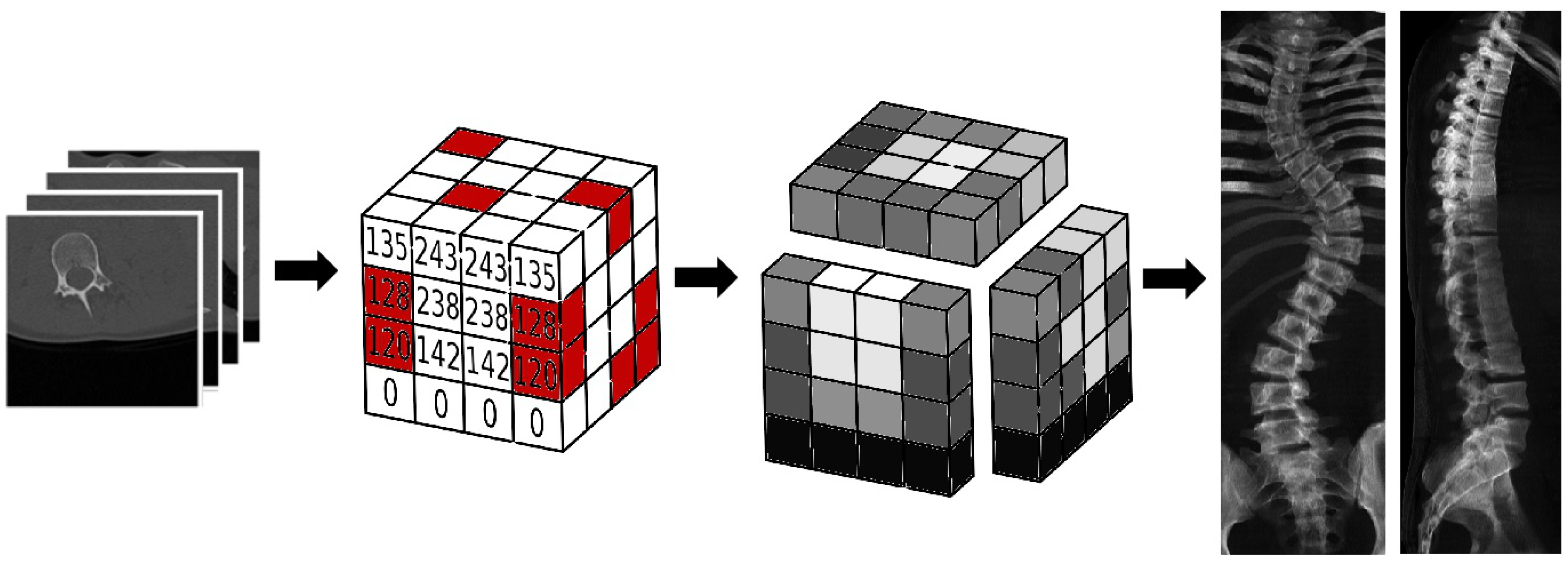
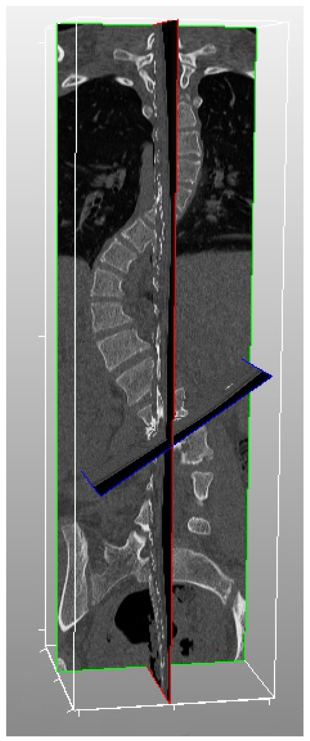
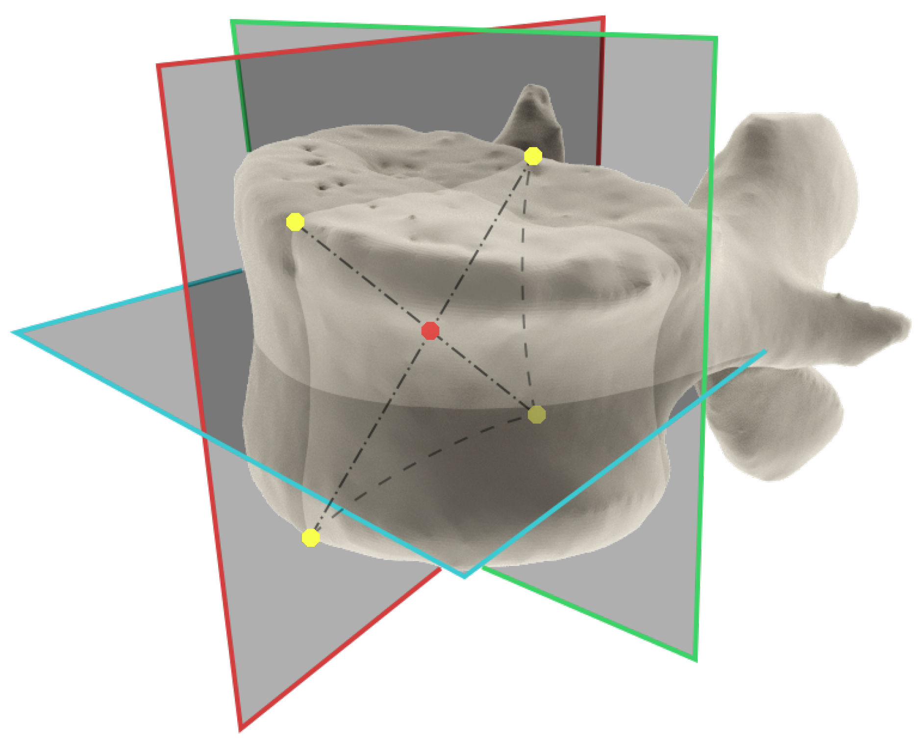
9]. CT scans are saved in DICOM file format. The information about location and spatial relations of structures is stored in form of voxels (a 3D pixels). The coordinates of voxels are predefined by the imaging system used. To obtain the central vertebral body points, one needs two sets of precise sections dissecting each vertebra. The section is not parallel to the upper or the lower vertebral lamina because the vertebra can be deformed by torsion [
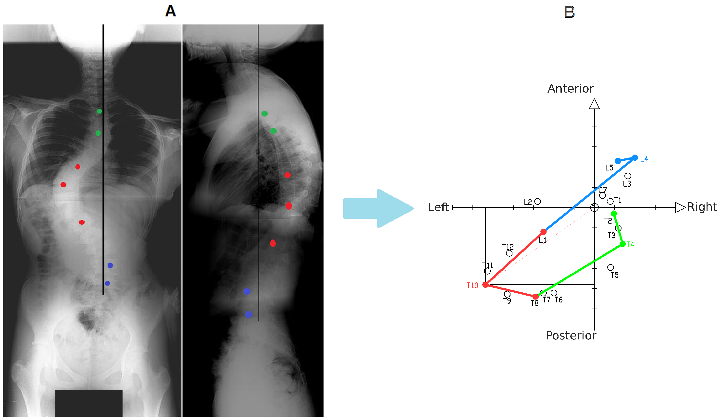
13]. In wedge shaped vertebra, the horizontal section parallel to the lower or the upper lamina does not dissect the vertebra body in half. The PNG file format was chosen for DRRs. PNG is a graphic data file format which uses lossless compression methods, as opposed to JPEG which loses some information and generates artifacts during compression. DEVIDE was used for vertebral column CT scans analysis. This software has the following characteristics: (1) it could present the vertebral column in three dissecting planes; (2) it allows marking points on each plane and extracting the coordinates; (3) it contains data export functionality (as separate file); (4) it supports DICOM and PNG files. The central vertebral points of lumbar part of the spinal column were easy to measure, even in case of scoliosis, on the X-rays. The size of lumbar vertebrae allow one to exactly mark their margins on both antero-posterior and sagittal images. Thoracic vertebrae are harder to asses because of the rib cage and bones of the upper extremity. Moreover when the angle of scoliosis is bigger one can observe that vertebral bodies can overlap on lateral images. Analysis of lateral images needed from observers a certain level of precision and knowledge in anatomical radiology. Analysis of AP images was much easier- even in severe scoliosis one can easily define the edges of vertebral bodies. The measurements of central vertebral points allow one to draw the Spine Axial Projection (SAP). SAP is a projection of spinal column onto the axial plane, it is a form of “Top View” [12,14,15]. It is a presentation of vertebrae and their relations in space on axial plane. The central coordinate point of the SAP represents SVA and CSL. SVA and CSL represent the axis of compensated vertebral column; SAP allows to measure the direction and amount of deformation against SVA and CSL, so one can define the direction and the amount of the whole spinal column deformity. The Spine Axial Presentation shows as a True da Vinci Projection the localization and relationships between vertebrae and End Apical End planes (EAE-planes) [
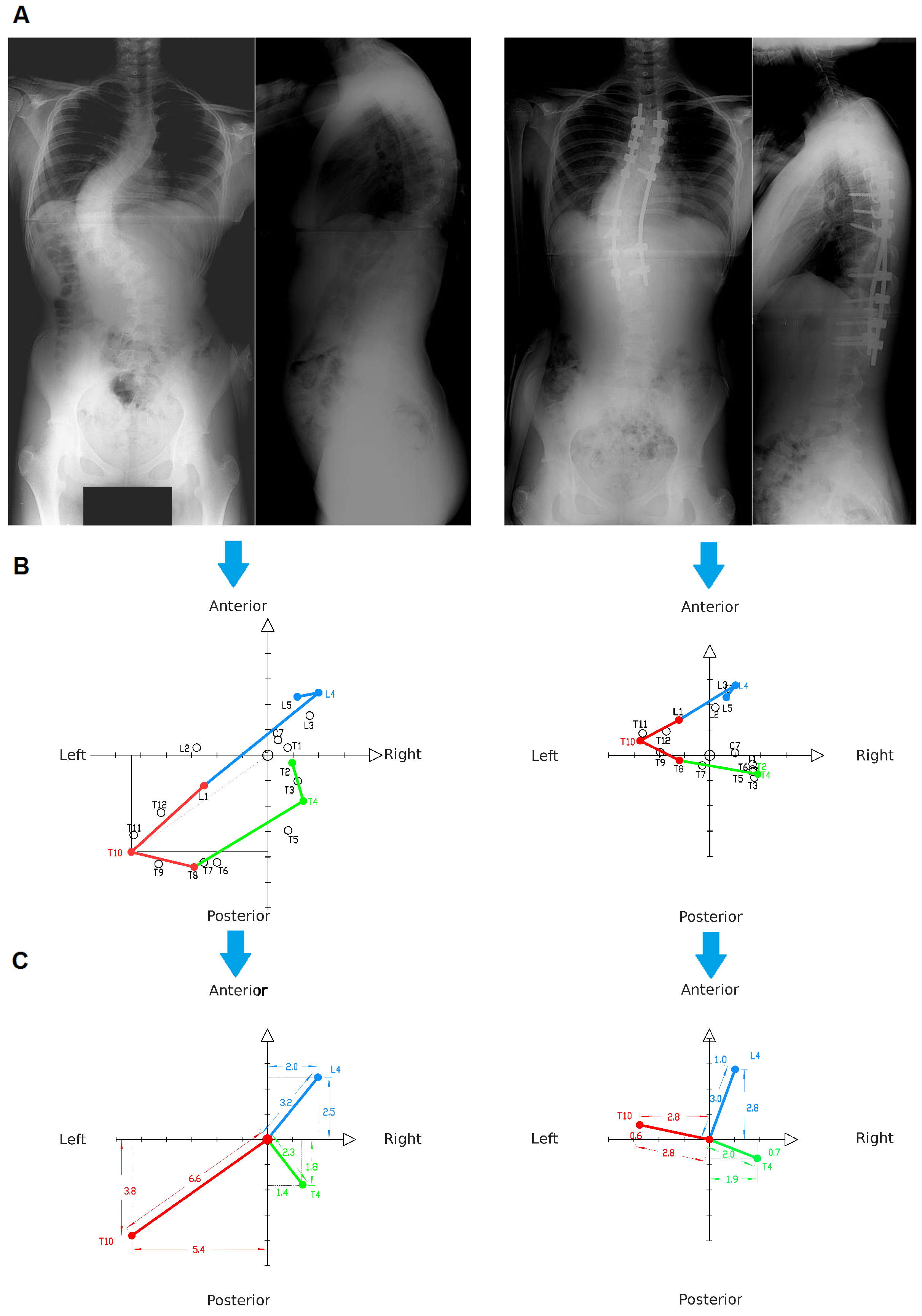
11]. As opposed to True da Vinci Projection, the SAP allows one to present the transverse top view of the spine without using the computer software. It could be done after measuring the distances between the central vertebral point, CSL and SVA. Spine Axial Presentation also provides information about the localization of EAE-planes. Drawing Spine Axial Presentation is time consuming, although it gives a surgeon additional information which, together with X-ray images, gives detailed knowledge of the whole deformity. It also allows patients to better understand their scoliotic deformities, so one can better explain planned treatment. Visual aids are important for good patient cooperation and patients’ improved understanding of their illness brings better patient outcomes. The patients are able to observe the deviation of vertebrae from their proper position and the direction in which the vertebrae are displaced (Figure 6).

6. Conclusions

Based on two standard radiographs, antero-posterior and lateral, it is possible to localize vertebral bodies in 3D space, getting additional information about scoliotic deformity of the spine. Graphical imaging of deformity in form of Spine Axial Presentation can be obtained manually, facilitating the understanding of the tree-dimensional character of scoliotic deformity. SAP allows one to assess the magnitude and direction of the acquired correction of scoliosis during the surgery (Figure 6). SAP also allows us to better assess the changes of curves in scoliosis during the brace treatment and progression.

Acknowledgments

This work was supported by The National Centre for Research and Development under the Grant No. PBS3/B9/34/2015.

Author Contributions

Paweł Główka, Dominik Gaweł and Tomasz Kotwicki designed the research. Dominik Gaweł and Michał Nowak developed the software. Paweł Główka and Bartosz Kasprzak did the measurements. Paweł Główka analyzed the data. Writing the paper was an equal team work. All authors have read and approved the final manuscript.

Conflicts of Interest

The authors declare no conflict of interest.

Abbreviations

The following abbreviations are used in this manuscript:
CTComputed Tomography
DRRDigitally Reconstructed Radiograph
SRSScoliosis Research Society
EOSbiplane Low-dose X-ray Imaging System
EAE-planesEnd-apical-end Planes
SAPSpine Axial Presentation
SVASagittal Vertical Axis
CVSLCentral Vertical Sacral Line
PNGPortable Network Graphic
DICOMDigital Imaging and Communications in Medicine
ITKThe Insight Segmentation and Registration Toolkit
VTKThe Visualization Toolkit
APAntero-posterior
LATLateral

References

  1. Hattori, T.; Sakaura, H.; Iwasaki, M.; Nagamoto, Y.; Yoshikawa, H.; Sugamoto, K. In vivo three-dimensional segmental analysis of adolescent idiopathic scoliosis. Eur. Spine J. 2011, 20, 1745–1750. [Google Scholar] [CrossRef] [PubMed]
  2. Stokes, I.A. Three-dimensional terminology of spinal deformity: A report rresented to the scoliosis research society by the scoliosis research society working group on 3-D terminology of spinal deformity. Spine 1994, 19, 236–248. [Google Scholar] [CrossRef] [PubMed]
  3. Kotwicki, T.; Negrini, S.; Grivas, T.B.; Rigo, M.; Maruyama, T.; Durmala, J.; Zaina, F. Methodology of evaluation of morphology of the spine and the trunk in idiopathic scoliosis and other spinal deformities-6th SOSORT consensus paper. Scoli. Spinal Disord. 2009, 4, 1. [Google Scholar]
  4. Kotwicki, T. Evaluation of scoliosis today: Examination, X-rays and beyond. Disabil. Rehabil. 2008, 30, 742–751. [Google Scholar] [CrossRef] [PubMed]
  5. Kim, H.; Kim, H.S.; Moon, E.S.; Yoon, C.S.; Chung, T.S.; Song, H.T.; Suh, J.S.; Lee, Y.H.; Kim, S. Scoliosis imaging: What radiologists should know. Radiographics 2010, 30, 1823–1842. [Google Scholar] [CrossRef] [PubMed]
  6. Ilharreborde, B.; Ferrero, E.; Alison, M.; Mazda, K. EOS microdose protocol for the radiological follow-up of adolescent idiopathic scoliosis. Eur. Spine J. 2016, 25, 526–531. [Google Scholar] [CrossRef] [PubMed]
  7. Morvan, G.; Mathieu, P.; Vuillemin, V.; Guerini, H.; Bossard, P.; Zeitoun, F.; Wybier, M. Standardized way for imaging of the sagittal spinal balance. Eur. Spine J. 2011, 20, 602–608. [Google Scholar] [CrossRef] [PubMed]
  8. McKenna, C.; Wade, R.; Faria, R.; Yang, H.; Stirk, L.; Gummerson, N.; Sculpher, M.; Woolacott, N. EOS 2D/3D X-ray imaging system: A systematic review and economic evaluation. Health Technol. Assess. 2012, 16, 1–188. [Google Scholar] [CrossRef] [PubMed]
  9. De Smet, A.A.; Tarlton, M.A.; Cook, L.T.; Berridge, A.S.; Asher, M.A. The top view for analysis of scoliosis progression. Radiology 1983, 147, 369–372. [Google Scholar] [CrossRef] [PubMed]
  10. Sangole, A.P.; Aubin, C.E.; Labelle, H.; Stokes, I.A.; Lenke, L.G.; Jackson, R.; Newton, P. Three-dimensional classification of thoracic scoliotic curves. Spine 2009, 34, 91–99. [Google Scholar] [CrossRef] [PubMed]
  11. Labelle, H.; Aubin, C.E.; Jackson, R.; Lenke, L.; Newton, P.; Parent, S. Seeing the spine in 3D: How will it change what we do? J. Pediatr. Orthop. 2011, 31, S37–S45. [Google Scholar] [CrossRef] [PubMed]
  12. Donzelli, S.; Poma, S.; Balzarini, L.; Borboni, A.; Respizzi, S.; Villafane, J.H.; Zaina, F.; Negrini, S. State of the art of current 3-D scoliosis classifications: A systematic review from a clinical perspective. J. Neuroeng. Rehabil. 2015, 12, 1. [Google Scholar] [CrossRef] [PubMed]
  13. Poncet, P.; Dansereau, J.; Labelle, H. Geometric torsion in idiopathic scoliosis: Three-dimensional analysis and proposal for a new classification. Spine 2001, 26, 2235–2243. [Google Scholar] [CrossRef] [PubMed]
  14. Kohashi, Y.; Oga, M.; Sugioka, Y. A new method using top views of the spine to predict the progression of curves in idiopathic scoliosis during growth. Spine 1996, 21, 212–217. [Google Scholar] [CrossRef] [PubMed]
  15. Negrini, S.; Atanasio, S.; Fusco, C.; Zaina, F.; Negrini, A. 3-DEMO Classification of Scoliosis: A Useful Understanding of the 3rd Dimension of the Deformity. Stud. Health Technol. Inform. 2008, 135, 139. [Google Scholar] [PubMed]
Figure 1. Two X-Rays images, AP and lateral (A) used for exemplary construction of the Spine Axial Presentation (SAP) (B). SAP can be obtained manually, on paper, without using any computer nor specialized software. The central point of the plot corresponds to the Central Vertical Sacral Line (CVSL) and the Sagittal Vertical Axis (SVA). Dots C7 to L5 represent the vertebral bodies central points. The Proximal minor curve is marked in green, the main curve is marked in red, the distal minor curve is marked in blue. The black dotted lines show the relationships of the main curve’s apical vertebrae with the coronal and the sagittal. The red dotted lines show the relationship of the apical vertebra with the Central Vertical Sacral Line and Sagittal Vertical Axis. The dots marked on the X-rays were magnified for visibility.
Symmetry 08 00125 g001
Figure 2. Schematic presentation of production of Digitally Reconstructed Radiograph from CT scans.
Symmetry 08 00125 g002
Figure 3. CT DICOM files opened with DeVide. The spine is visualized in three planes that dissect each other. The angles between those planes can be manually adjusted.
Symmetry 08 00125 g003
Figure 4. The method of obtaining the vertebral body central point based on computer tomography (CT) scans. The figure shows how the planes were positioned in relation to the vertebral body. The vertebral body central point is obtained by crossing the lines connecting the dots marked on vertebral body corners seen in the sagittal cross-section.
Symmetry 08 00125 g004
Figure 5. Procedure for obtaining the central vertebral body points based on digitally reconstructed radiographs (DRRs). First the corners of the vertebral bodies contours are marked. Next, these points are connected. The point where the lines crossed is defined as a vertebral body central point. Based on digitally reconstructed antero-posterior radiographs (AP DRR) the x, z coordinates are obtained. Based on lateral DRR the y, z coordinates are obtained.
Symmetry 08 00125 g005
Figure 6. Left side presents the pre-surgery status. Right side presents the post-surgery status. The figure shows antero-posterior and lateral X-rays (A) and Spine Axial Presentations obtained on their basis (B). The position of vertebral bodies central points is indicated by the dots. The curves for the EAE planes are marked: proximal minor curve in green, main curve in red, distal minor curve in blue. SAPs shows the change of the vertebral bodies position. Both the pre-oper and post-oper Spine Axial Presentation allow for assessment magnitude of the acquired correction of scoliosis during the surgery. The figure shows the position of apical vertebral bodies central points in relation to sagittal plane (anterior-posterior axis), frontal plane (left-right axis) and CSL (C).
Symmetry 08 00125 g006
Table 1. Patient’s data. F- female, M- male.
No.Gender M/FAgeLenke TypePrimary CurveSuperior CurveInferior CurveNo. of Vertebrae Analyzes
1F151C -79605518
2F141B N88715317
3F71A N77364416
4M91A -71364217
5F171B -88425417
Average-12.4-76.852.849.617
Total------85
Table 2. Intraobserver reproducibility and Interobserver reliability for x, y and z coordinates of vertebral bodies centers based on CT imaging , p = 0.05.
Intraobserver ReproducibilityInterobserver Reliability
CT CoordinatesICCMean Difference (mm)Standard Error of Mean Difference for One MeasurementICCMean Difference (mm)Standard Error of Mean Difference for One Measurement
x0.99850.060.160.98150.320.58
y0.99600.450.210.99600.540.2
z0.99742.990.780.99752.870.77
Table 3. Intraobserver reproducibility and Interobserver reliability for x, y and z coordinates of vertebral bodies centers based on DRR, p = 0.05.
Intraobserver ReproducibilityInterobserver Reliability
DRR CoordinatesICCMean Difference (mm)Standard Error of Mean Difference for One MeasurementICCMean Difference (mm)Standard Error of Mean Difference for One Measurement
x0.99700.191.020.90041.31.32
y0.99600.310.210.99460.190.24
z0.99630.220.130.99691.051.28
Table 4. Intraobserver reproducibility and Interobserver reliability for z coordinate of vertebral bodies centers based on DRR of antero-posterior (AP) and lateral (LAT) projection, p = 0.05.
Intraobserver ReproducibilityInterobserver Reliability
DRR ‘z’ CoordinateICCMean Difference (mm)Standard Error of Mean Difference for One MeasurementICCMean Difference (mm)Standard Error of Mean Difference for One Measurement
Z AP0.99590.220.130.99401.051.28
Z LAT0.99675.411.660.99970.310.29
Z AP vs LAT0.99634.361.020.99694.240.28
Table 5. Intraobserver reproducibility and Interobserver reliability single measures for comparison x, y and z coordinates of vertebral bodies centers based on CT and DRR imaging, p = 0.05.
Intraobserver ReproducibilityInterobserver Reliability
CT / DRR CoordinatesICCMean Difference (mm)Standard Error of Mean Difference for One MeasurementICCMean Difference (mm)Standard Error of Mean Difference for One Measurement
x0.99111.020.190.98770.260.46
y0.99730.150.130.98820.240.14
z0.99980.090.260.99980.290.25

