Big Bounce Genesis and Possible Experimental Tests: A Brief Review

Abstract

We review the recent status of big bounce genesis as a new possibility of using dark matter particles’ mass and interaction cross-section to test the existence of a bounce universe at the early stage of evolution in our currently-observed universe. To study the dark matter production and evolution inside the bounce universe, called big bounce genesis for short, we propose a model independent approach. We shall present the motivation for proposing big bounce, as well as the model independent predictions, which can be tested by dark matter direct searches. A positive finding shall have profound impact on our understanding of the early universe physics.

1. Motivation and Overview

Understanding the working principles of fundamental constituents pivots on the knowledge of the origin of the universe [1]. Cosmology is therefore the oldest intellectual pursuit of mankind. The inflationary paradigm is the laurel of modern cosmology as it solves in one stroke the monopoles, horizon and flatness problems of the Big Bang Cosmology (BBC) by modelling a brief period of exponential expansion after the Big Bang using simple scalar fields [2]. It turns out that a nearly scale-invariant primordial power spectrum, which agrees well with the current array of Cosmic Microwave Background (CMB) observations [3,4], can be generated from the quantum fluctuations of the scalar field in the simplest inflation model [5]. This achievement is crowned the “inflation paradigm”.

Slowly, it dawns on some cosmologists that, similar to the BBC, the scenario of inflation also suffers from its own problems, the initial singularity problem and the fine-tuning problem [6].

The challenge presents great opportunities in developing new theories for the early universe. In the past decade in a concordal effort to resolve the initial singularity problem of the inflation scenario, the “bounce universe scenario” (BUS) was proposed by postulating a phase of contraction before the universe turns around, called the Big Bounce in lieu of the Big Bang (recent reviews can be found in [7,8,9,10]).

Efforts on detailed implementations ensue with many working models of the Big Bounce universe proposed [11,12,13,14,15,16,17,18,19,20,21,22,23,24,25,26,27,28,29,30,31,32,33,34,35,36,37,38,39,40,41,42,43,44,45,46,47,48]. According to the BUS, our universe is bouncing from a contracting phase to an expanding phase at non-zero minimum size, so the Big Bang Singularity is resolved. The horizon problem and flatness problems are solved by observing that there is an interplay of the physical scale and the Hubble scale similar to the inflationary scenario, as depicted in Figure 1.

The solution to the Big Bang problems—horizon, flatness and homogeneity—by the coupled scalar tachyon fields bouncing universe(CSTB) model is explicitly demonstrated in a recent paper [34].

Moreover, a stable, as well as scale-invariant power spectrum of primordial density perturbations matching the currently-observed CMB spectra can be obtained during the phase of matter-dominated contraction in the BUS [49,50,51,52].

In light of such fast developments, we are well motivated to work out further criteria for testing the bounce universe models and extract discriminating predictions to distinguish the bounce scenario from the inflationary paradigm. Even though the details of cosmic evolution in the inflation scenario and BUS are so different, the experimental or observational evidence, which can be used to tell these two models apart, is still lacking. One may expect that the precisely-measured CMB spectra are suitable to distinguish these two scenarios. However, they are still not enough to concretely distinguish these two scenarios due to the following two factors [53]:

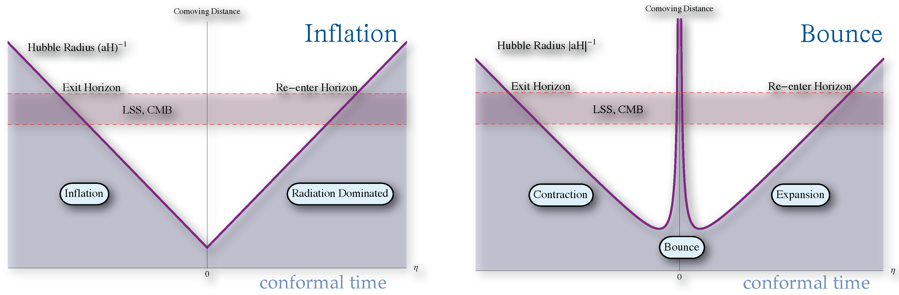
• In terms of the primordial power spectrum, a complete duality between the inflation scenario and BUS has been well established [49,50,51,54,55]. It enables both inflation and BUS to generate a scale-invariant primordial power spectrum with the same probability from the unified parameter space. In short, if a primordial power spectrum can be generated in an expanding phase of cosmological evolution, it can also be generated in a contracting phase with the same scale dependence and time dependence [51]. Literally, they are degenerate in the leading-order signatures of CMB spectra;
• Currently, all models in these two scenarios are utilizing some undetected classical/quantum fields to drive the inflation or big bounce at the very early stage of cosmic evolution. Hence, their predictions of the CMB spectrum and the scalar-tensor ratio, both built on the linear perturbation theory of these unconfirmed fields, are still questionable.

Therefore, the usual temperature-temperature correlations and scalar to tensor ratio in the CMB spectrum cannot serve as direct evidence for either the inflation scenario or BUS. Hence, new concrete methods, independent of CMB observations, for distinguishing the inflation scenario and BUS with falsifiable predictions are urgently needed. That is where our proposal [56] dubbed “Big Bounce Genesis” steps in, in which dark matter (DM) direct detection experiments are proposed to be a testing ground to distinguish the bounce universe scenario from the inflation paradigm.

Big Bounce Genesis (BBG) [56] is a framework for analysing matter production and evolution in the bounce universe, in which there is a period of contraction prior to the a period of expansion connected by a bounce. By incorporating the concept of weak freeze-out, an explicit computation in out-of-chemical equilibrium productions of DM shows that the cross-section and DM mass are constrained by the observed relic abundance of DM, ${\mathsf{\Omega }}_{\chi }$ [56]:

$${\mathsf{\Omega }}_{\chi }\propto {\langle \sigma v\rangle }_{\chi }{m}_{\chi }^2.$$

(1)

This relation is depicted by Curve B in Figure 2. This characteristic relation is significantly different from the standard cosmology predictions:

$${\mathsf{\Omega }}_{\chi }\propto {\langle \sigma v\rangle }_{\chi }^{-1}{m}_{\chi }^0,$$

(2)

in either the WIMP or WIMP-less miracles [57,58,59,60], as depicted by Curve A in Figure 2.

The existence of this relation can therefore be a telling sign that the universe has gone through a Big Bounce [56].

Therefore one can be hopeful that data from current and future DM detections can tell these two early universe scenarios apart [61]. A confirmed relation between DM mass and the interaction cross-section not only can lend support to the idea that the cosmos goes through a bounce and not a bang, but also establishes the one-way production of matter in the early universe. All of these shall have profound implications in early universe physics.

In BBG [53,56,62], DM particles are assumed to be produced by the annihilation of Standard Model(SM) particles in hot plasma of the bounce cosmological background. The following model independent interaction is assumed,

$$\varphi +\varphi ⟺\chi +\chi$$

(3)

where ϕ denotes SM particles and χ denotes DM particles (can be either fermions or bosons). This assumption leaves DM mass, $m_{\chi }$, and the cross-section, $\langle \sigma v\rangle$, as two free parameters constrained by the astrophysical observations.

In a model independent analysis of the bounce universe dynamics, we divide the cosmic evolution of a generic bounce universe schematically into three stages: Phase I: pre-bounce contraction; Phase II: post-bounce expansion; and Phase III: freeze-out phase; as shown in Figure 3.

If DM is produced efficiently in both of the pre-bounce contraction and post-bounce expansion when the background temperature is high and the duration is long enough. The freeze-out process of DM commences after the post-expansion. Generically, such a thermal production mechanism is model independent and irrelevant to the details of the realization of bounce since the bounce point connecting Phase I and Phase II is assumed too short to affect DM productions [53,63].

For the production of DM, there are two different avenues, thermal equilibrium production and out-of-chemical equilibrium production.

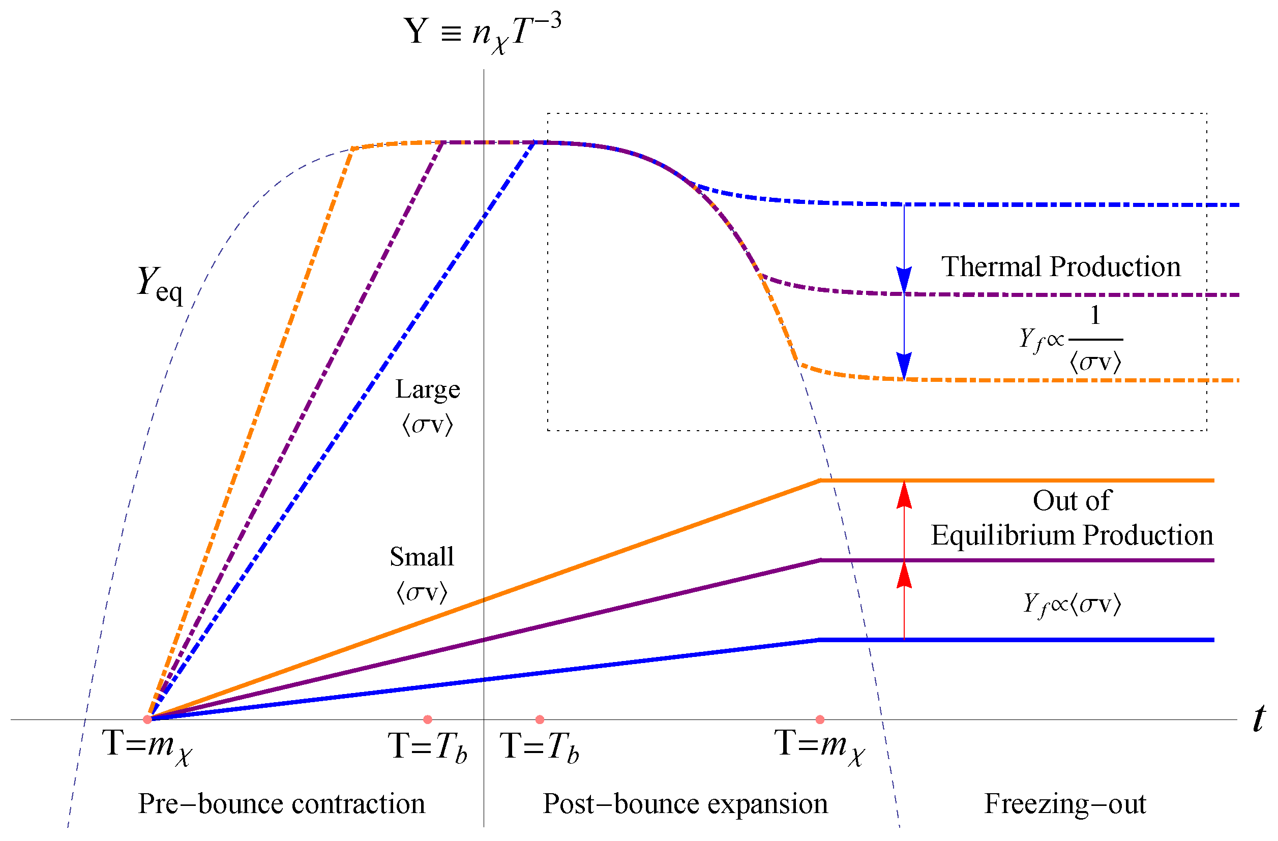
• Thermal equilibrium production: DM particles with large cross-sections are produced very efficiently, so that their abundance increases rapidly and achieves the thermal equilibrium value even in the pre-bounce contracting or post-bounce expanding phases. Then, the abundance of DM tracks the thermal equilibrium value before the freeze-out takes place,

  $$Y\left(t\right)=Y_{eq},t<t_f,$$

  (4)

  where $Y\equiv \frac{n_{\chi }}{T^3}$ is the abundance of DM, $Y_{eq}$ is the thermal equilibrium abundance in the given cosmological background with temperature T and $t_f$ is the moment of the freeze-out commencing.
• Out-of-chemical equilibrium production [56]: In a given cosmological background, if the cross-section of DM is small enough, the production of DM should be inefficient. Therefore, its abundance cannot achieve the thermal equilibrium value during the production process,

  $$Y\left(t\right)\ll Y_{eq},t<t_f.$$

  (5)

Additionally, for the freeze-out process, there are also two different means. At the end of Phase II: post-bounce expansion, the background temperature continues to fall as long as the universe is expanding; the forward reaction of Equation (3) is suppressed exponentially, i.e., the production of DM ends. Depending on the abundance of DM at this moment, this freeze-out process of DM can be categorized into two types: strong freeze-out and weak freeze-out [56].

• Strong freeze-out: If plenty of DM particles have been produced before, the backward reaction of Equation (3) dominates, as the forward reaction of Equation (3) is suppressed exponentially. The backward reaction decreases the abundance of DM very efficiently until the number density of DM is too low to keep thermal contact in the expanding phase. Therefore, after such a strong freeze-out, the relic abundance of DM is significantly lower than that before freeze-out and is inverse to the DM cross-section,

  $$Y_f\propto \frac{1}{\langle \sigma v\rangle },$$

  (6)

  where $Y_f$ is the relic abundance of DM after freeze-out, $t\ge t_f$. This is just the well-known freeze-out process in the WIMP and WIMP-less miracle [57,58], and we label it as “strong freeze-out” compared with the “weak freeze-out” as follows.
• Weak freeze-out: If the abundance of DM is very low, the backward reaction in Equation (3) is always negligible. When the forward reaction in Equation (3) is suppressed exponentially, both the production and annihilation of DM end. Therefore, the relic abundance of DM is equal to the abundance of DM at the end of the production phases and is generically proportional to the DM cross-section,

  $$Y_f=Y\left(t_f\right)\propto \langle \sigma v\rangle .$$

  (7)

  Remarkably, since all of the abundance of DM, which is sensitive to cosmological evolution, is preserved, such a relic abundance of DM undergoing the weak freeze-out process is encoded with information of the early evolution of the universe.

In view of the two possible production routes and the subsequent two possible freeze-out processes of DM, there arise four possibilities, as displayed in

Table 1. Production and freeze-out of DM in “bounce universe scenario” (BUS).

	Thermal Equilibrium Production	Out-of-Chemical Equilibrium Production
Strong freeze-out	Route I	—
Weak freeze-out	Route III	Route II

.

The time evolution of DM in a generic bounce cosmos is illustrated in Figure 4, respectively for Route I and Route II. In the following discussion, we take DM as a bosonic particle and the highest temperature of the bounce larger than the mass of DM (in this case, Route III is not manifest, and we discuss the details of Route III in the next section.).

In Route I of BBG, DM is produced through thermal equilibrium production and undergoes strong freeze-out. DM commences its thermal decoupling from the thermal equilibrium state and, eventually, freezes out with the relic abundance inverse to its cross-section. Therefore, the relic abundance of DM predicted by Route I is identical to the prediction of the models in the standard inflationary cosmology, such as the WIMP and WIMP-less miracles [56,57,58]. Particularly, the WIMP and WIMP-less miracles can be viewed as a part of this process; see the dashed black frame in Figure 4. The relation of cross-section and mass predicted by this case is the Branch A in Figure 2.

The novelty appears in Route II, out-of-chemical equilibrium production and weak freeze-out. During the production phase, the abundance of DM is much lower than the value of the thermal equilibrium state. With the falling of the temperature of background, DM takes a very weak freeze-out process that all pieces of information of the early universe evolution are preserved in the relic abundance of DM, which leads to a new characteristic relation of the DM cross-section and mass that is compatible with current observations ( Branch B in Table II of [56]),

$$\langle \sigma v\rangle =7.2\times {10}^{-26}{m}_{\chi }^{-2},m_{\chi }\gg 432\mathrm{eV}$$

(8)

where $\langle \sigma v\rangle$ is the thermally-averaged cross-section of DM. This relation of cross-section and mass is shown as Branch B in Figure 2. As a smoking gun signal for the existence of the bounce universe, this novel relation can be used to check against recent and near future data from experiments of DM to determine whether or not the universe undergoes a big bounce at a very early stage of cosmic evolution [61,64].

In general, the production and evolution of DM in the bounce cosmos (Big Bounce Genesis for short) brings about new possibilities, compared to the standard model particle physics in the standard cosmology, which are listed in

Table 2. Categories of Big Bounce Genesis (BBG) models.

	High Temperature Bounce	Low Temperature Bounce
	${\mathit{T}}_{\mathit{b}}\mathbf{\gg }{\mathit{m}}_{\mathit{\chi }}$	${\mathit{T}}_{\mathit{b}}\mathbf{\ll }{\mathit{m}}_{\mathit{\chi }}$
Bosonic Dark Matter	Type I	Type III
Fermonic Dark Matter	Type II	Type IV

. The generic picture of BBG is illustrated with the model of the evolution of scalar DM in a high temperature bounce.

In each of the venues listed in Table 2, DM is produced and evolves through different routes listed in Table 1 and gives (beyond standard model) predictions. In this review, we discuss each case in detail.

This review is organized as follows: In Section 2, we discuss each type of BBG dynamics following [53,56,62]. We study the generation of thermal fluctuations of DM in the bounce cosmos following [65] and show that the bounce dynamic is stable against thermal fluctuations for $T_{bounce}\le T_{Planck}$, in Section 3. In Section 4, we discuss the search of BBG DM in direct detection experiments for mass range DM mass$\sim 100$ GeV using nuclear recoil [61] and for light DM by electron recoil [64].

2. Dark Matter Production and Evolution in the Bounce Universe Scenario

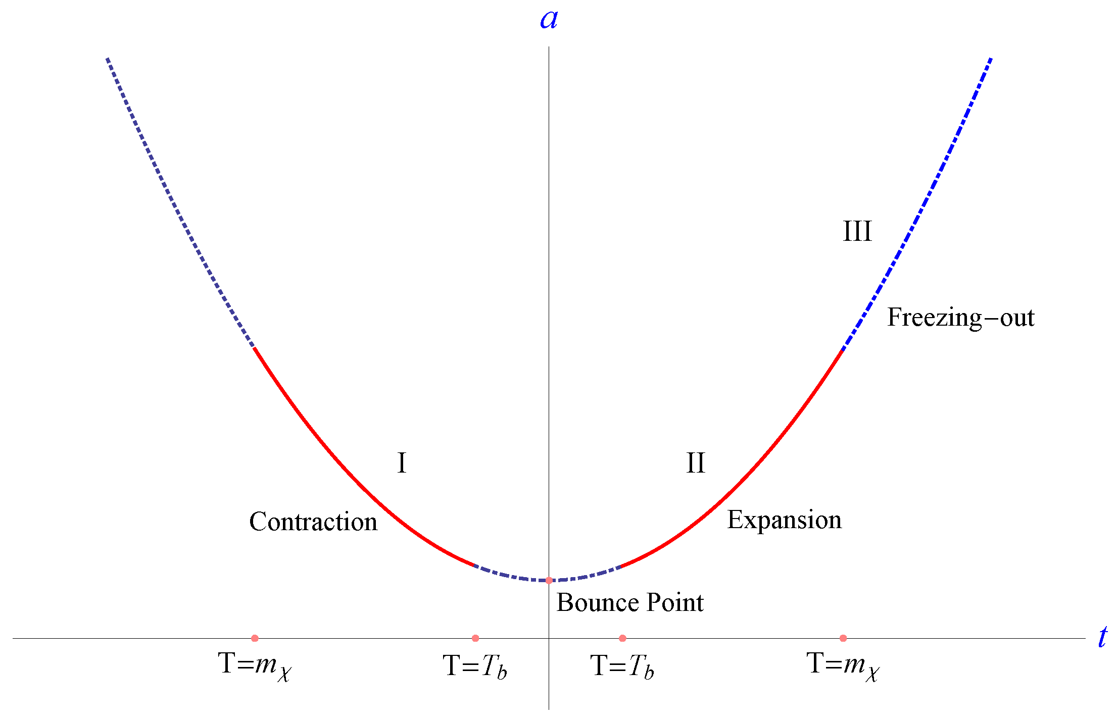
In general, the evolution of DM in BUS is governed by the Boltzmann equation,

$$\frac{d\left(n_{\chi }{a}^3\right)}{a^{3}dt}=\widetilde{\langle \sigma v\rangle }\left[{\left(n_{\chi }^{eq}\right)}^2-n_{\chi }^2\right],$$

(9)

where $n_{\chi }^{eq}$ is the thermal equilibrium number density of DM, a the scale factor of the cosmological background and $\widetilde{\langle \sigma v\rangle }$ the thermally-averaged cross-section with temperature dependence. Since the DM mass is large, the production phases of DM is radiation-dominated,

$$\rho \propto a^{-4}\propto T^4,$$

(10)

where ρ is the energy density of the cosmological background. To facilitate the study of the whole evolution of DM in a generic bounce cosmos, without loss of generality, we take the following two conditions,

• Initial abundance of DM takes $n_{\chi }^i=0$, i.e., the number density of DM is set to be zero at the onset of the pre-bounce contraction phase in which $T\ll m_{\chi }$.
• The matching condition on the bounce point is $n_{\chi }^{+}\left(T_b\right)=n_{\chi }^{-}\left(T_b\right)$, i.e., the number density of DM, $n_{\chi }$, at the end of the pre-bounce contraction (denoted by −) is equal to the initial abundance of the post-bounce expansion (denoted by +), given that the entropy of the universe is conserved around the bounce point [63].

Therefore, by solving Equation (9) with these two conditions, the evolution of DM abundance is fully determined. Then, we can obtain the characteristic relations of DM cross-section and mass for each type of BBG model constrained by the recent observational energy fraction of DM, ${\mathsf{\Omega }}_{\chi }=0.26$.

2.1. Type I: Scalar Dark Matter in a High Temperature Bounce

Following [56], the simplest case is that the highest temperature of bounce is larger than the DM mass, $T_b\gg m_{\chi }$, and both χ and ϕ are scalar particles. Thus, the interactions of DM with the light boson can be modelled by ${\mathcal{L}}_{int}=\lambda {\varphi }^2{\chi }^2$. Additionally, in the limit $m_{\varphi }\to 0$, we get [66],

$$\widetilde{\langle \sigma v\rangle }=\left\{\begin{array}{c}{\displaystyle \frac{x^2}{4}·\langle \sigma v\rangle ,m_{\chi }\ll T}\hfill \\ \\ {\displaystyle \langle \sigma v\rangle ,m_{\chi }\gg T}\hfill \end{array}\right.,x\equiv \frac{m_{\chi }}{T},\langle \sigma v\rangle =\frac{1}{32\pi }\frac{{\lambda }^2}{m_{\chi }^2}.$$

(11)

Substituting Equation (11) and (10) into Equation (9), the Boltzmann equation can be simplified during the production phases,

$$\frac{d{Y}_{\mp }}{dx}=\mp f\langle \sigma v\rangle m_{\chi }(1-{\pi }^4{Y}_{\mp }^2),x<1,$$

(12)

where ∓ denotes the pre-bounce contraction and post-bounce expansion, respectively, $T\gg m_{\chi }$ , and f is a constant during these phases with $f\equiv \frac{m_{\chi }^2}{4{\pi }^2}(|H|x^2{)}^{-1}=1.5\times {10}^{26}$ eV, being constrained by recent astrophysical observations. Then, by solving Equation (12) with the initial abundance of DM and the matching condition on the bounce point, the complete solution of the DM abundance in the post-bounce expansion is obtained,

$$Y_{+}=\frac{1-e^{-2{\pi }^{2}f\langle \sigma v\rangle m_{\chi }(1+x-x_b)}}{{\pi }^2\left(1+e^{-2{\pi }^{2}f\langle \sigma v\rangle m_{\chi }(1+x-2x_b)}\right)}.$$

(13)

At the end of DM production, T∼$m_{\chi }$, this solution can be categorized into two limits, thermal equilibrium production and out-of-chemical equilibrium production,

$$Y_{+}{|}_{x=1}=\left\{\begin{array}{c}{\displaystyle {\pi }^{-2},4{\pi }^{2}f\langle \sigma v\rangle m_{\chi }\gg 1}\hfill \\ {\displaystyle 2f\langle \sigma v\rangle m_{\chi },4{\pi }^{2}f\langle \sigma v\rangle m_{\chi }\ll 1}\hfill \end{array}\right..$$

(14)

They are the two venues of DM production discussed in the last section.

• Thermal equilibrium production: For the upper line in Equation (14), with the large value of $\langle \sigma v\rangle m_{\chi }$, DM is produced in abundance, which has reached the thermal equilibrium before the end of the production phases.
• Out-of-chemical equilibrium production: Additionally, for the lower line in Equation (14) with the small value of $\langle \sigma v\rangle m_{\chi }$, the production is mostly one-way, and thermal equilibrium cannot be established, so that its abundance is much lower than the value of the thermal equilibrium state even at the end of he production phases.

After the production phases in which $x\le 1$, the cosmos is still in expansion, and the background temperature of universe continues to fall. The production of DM is exponentially suppressed, and thermal decoupling commences. To determine the relic abundance of DM after freeze-out, we solve the Boltzmann equation Equation (9) in the low temperature region,

$$\frac{dY}{dx}=4f\langle \sigma v\rangle m_{\chi }\left(\frac{\pi }{8}x{e}^{-2x}-{\pi }^4\frac{Y^2}{x^2}\right),x\ge 1$$

(15)

where the first term on the right-hand side of Equation (15) is subdominant and, hence, discarded for $x>1$. Integrating it from $x=1$ to $x\to \infty$, we obtain the relic abundance of DM after freeze-out,

$$Y_f\equiv {Y|}_{x\to \infty }=\frac{1}{4{\pi }^{4}f\langle \sigma v\rangle m_{\chi }+{\left(Y_{+}{|}_{x=1}\right)}^{-1}},$$

(16)

which leads to two distinctive outcomes of the freeze-out process:

• Strong freeze-out: If $Y_{+}{|}_{x=1}\gg {\left(4{\pi }^{4}f\langle \sigma v\rangle m_{\chi }\right)}^{-1}$, the initial abundance of DM at the onset of the freeze-out process is large enough for pair-annihilation of DM particles during the thermal decoupling, so that the relic abundance of DM becomes irrelevant of the initial abundance. Particularly, it is inversely proportional to the cross-section,

  $$Y_f=\frac{1.71\times {10}^{-29} e{V}^{-1}}{\langle \sigma v\rangle m_{\chi }}.$$

  (17)
• Weak freeze-out: If, on the other hand, $Y_{+}{|}_{x=1}\ll {\left(4{\pi }^{4}f\langle \sigma v\rangle m_{\chi }\right)}^{-1}$ and the density of DM is too low to pair-annihilate during the thermal decoupling. The relic abundance of DM after freeze-out in this limit is just the initial abundance at the onset of the freeze-out process,

  $$Y_f=Y_{+}{|}_{x=1}.$$

  (18)

Notice that two criteria for production from Equation (14) and for the freeze-out process from Equation (16) are mostly coincident. Therefore, Route III, thermal equilibrium production and weak freeze-out, is not manifest in the Type I model of BBG. In this model, if DM is produced in thermal equilibrium, it must undergo strong freeze-out; and if DM is produced through the out-of-chemical equilibrium production, it must undergo weak freeze-out, i.e., only Route I and Route II are viable.

For Route I, as the abundance of DM tracks the thermal equilibrium values during the production phase and the freeze-out phase, all information of the early universe encoded in the relic abundance of DM is washed out. This is analogous to the standard cosmology in which DM freezes out strongly from equilibrium [59], in both the WIMP miracle scenario [57] and the WIMP-less miracle scenario [58]. Therefore, the standard model and the bounce universe cannot be distinguished from each other as long as DM is produced at thermal equilibrium, depicted in Branch A of Figure 2.

In the production of Route II, the abundance of DM has not reached thermal equilibrium and, therefore, has not been suppressed by the “thermal envelop”, and its final abundance is directly proportional to its interaction cross-sections:

$$Y_f=Y_{+}{|}_{x=1}=3\times {10}^{26} \mathrm{eV}\langle \sigma v\rangle m_{\chi },$$

(19)

where we have used Equation (14). The relic abundance of DM produced this way encodes the information of the early universe dynamics when we reconstruct its decoupling time from its interaction cross-section. Utilizing the current observed value of ${\mathsf{\Omega }}_{\chi }$,

$${\mathsf{\Omega }}_{\chi }=1.18\times {10}^{-2} \mathrm{eV}\times m_{\chi }{Y}_f=0.26,$$

(20)

the DM relic abundance is constrained. This in turn forces the DM mass and cross-section to lie on the characteristic relation, Equation (8), depicted as the Branch B in Figure 2.

If the DM mass and its interaction cross-section are found to be related, as one point in Branch B, by (in)direct detection of DM, we can confidently conclude that the matter is produced in the early universe out-of-thermal equilibrium. This is in fact shared by many non-standard universe models based on $f\left(R\right)$ gravity [67,68] and on Galileon field [69,70,71].

2.2. Type III and IV: Bosonic and Fermionic Dark Matter in a Low Temperature Bounce

In a low temperature bounce, $T_b\ll m_{\chi }$, the DM is expected to be produced inefficiently. Therefore, we focus on (On the other hand, if the factor $f{\langle \sigma v\rangle }_0{m}_{\chi }$ is very large and $x_b\equiv \frac{m_{\chi }}{T_b}\to \mathcal{O}\left(1\right)$, the production of DM would be very efficient, so that the abundance of DM is able to achieve its thermal equilibrium; in this case, see [56].) the route in which DM is produced in out-of-chemical equilibrium and undergoes weak freeze-out, i.e., Route II listed in Table 1, following [56,62].

During a low temperature bounce, $x_b\gg 1$, the thermally-averaged cross-section of DM, $\widetilde{\langle \sigma v\rangle }$, becomes irrelevant with respect to temperature at the leading order,

$$\widetilde{\langle \sigma v\rangle }={\langle \sigma v\rangle }_0+\mathcal{O}\left(x^{-1}\right),$$

(21)

where ${\langle \sigma v\rangle }_0$ is simply determined by the interacting coupling constant of the DM particle [60]. Here, we approximate $\widetilde{\langle \sigma v\rangle }={\langle \sigma v\rangle }_0$ for simplicity. By utilizing the dimensionless abundance of DM, $\tilde{Y}\equiv n_{\chi }{s}^{-1}$, with the entropy density, s, the Boltzmann equation can be simplified further as follows,

$$\frac{d{\tilde{Y}}_{\mp }}{dx}=-\frac{s}{xH}{\langle \sigma v\rangle }_0\left({\tilde{Y}}_{\mp }^2-{\tilde{Y}}_{eq}^2\right)$$

(22)

where the subscript ∓ corresponds to the sign of the Hubble parameter, i.e., the contracting phase and expanding phase of a generic bounce universe, respectively. The entropy density is given by $s=(2{\pi }^2/45)h_{\star }{T}^3$ with $h_{\star }$ being the relativistic degree of freedom for the entropy density. In the radiation-dominated era, the Hubble parameter is proportional to $T^2$, $H=\frac{\pi T^2}{M_p}\sqrt{\frac{g_{\star }}{90}}$, where $g_{\star }$ and $M_p$ are, respectively, the relativistic degree of freedom of energy density and the reduce Planck mass.

In the low temperature limit $x\gg 1$, the thermal equilibrium number density of DM is suppressed exponentially by x, $n_{eq}=g_{\chi }{\left(m_{\chi }^2/2\pi x\right)}^{\frac{3}{2}}{e}^{-x}$, with $g_{\chi }$ being the number of degrees of freedom of χ. Thus, the particle creation term, ${\tilde{Y}}_{eq}^2$, on the right-hand of Equation (22) is suppressed exponentially by $2x$, ${\tilde{Y}}_{eq}^2\propto e^{-2x}$. Therefore, the production of DM can be expected to be very inefficient during such a low temperature bounce, so that the abundance of DM is unlikely able to achieve its thermal equilibrium value. Under this consideration, we focus on this out-of-thermal equilibrium case for the DM production, $\tilde{Y}\ll {\tilde{Y}}_{eq}$, i.e., the annihilation term ${\tilde{Y}}_{\mp }^2$ on the right-hand of Equation (22) can be dropped out in the following calculations.

By integrating Equation (22) with the initial condition ${\tilde{Y}}_{-}^i=0$ and the match condition ${\tilde{Y}}_{-}\left(x_b\right)={\tilde{Y}}_{+}\left(x_b\right)$, we obtain the relic abundance of DM (cf. Equation (3.3) in [62], which was firstly obtained in [56]):

$${\tilde{Y}}_f={\tilde{Y}}^{+}(x\gg x_b)=\mathcal{C}{\langle \sigma v\rangle }_0{m}_{\chi }{e}^{-2x_b}(1+2x_b).$$

(23)

where $\mathcal{C}=0.014M_p{g}_{\star }^{-\frac{1}{2}}{h}_{\star }^{-1}{g}_{\chi }^2$. By taking $g_{\chi }=1$ and $h_{\star }\simeq g_{\star }=90$ during the phases under consideration, $\mathcal{C}=6.9\times {10}^{22}$ eV. Imposing the currently-observed value of ${\mathsf{\Omega }}_{\chi }$,

$${\mathsf{\Omega }}_{\chi }=5.7\times {10}^8{m}_{\chi }{\tilde{Y}}_f{\mathrm{GeV}}^{-1}=0.26,$$

(24)

leads precisely to observational constrains on ${\langle \sigma v\rangle }_0$, $m_{\chi }$ and $x_b$,

$${\langle \sigma v\rangle }_0{m}_{\chi }^2{e}^{-2x_b}(1+2x_b)=6.6\times {10}^{-24}.$$

(25)

To sum up, by utilizing these observational constraints, the highest temperature of bounce can be determined in this scenario with the given value of $({\langle \sigma v\rangle }_0,m_{\chi })$.

2.3. Type II: Fermionic Dark Matter in a High Temperature Bounce

Following [62], in high temperature bounce $T_b\gg m_{\chi }$, the thermally-averaged cross-section of DM, $\widetilde{\langle \sigma v\rangle }$, can be parameterized as follows,

$$\widetilde{\langle \sigma v\rangle }={\tilde{\sigma }}_0{x}^{-n},x<1$$

(26)

where $n>0$ and typically, $n=2$ for the pair annihilation processes of Dirac and Majorana fermions into a pair of massless fermions, and ${\tilde{\sigma }}_0$ is simply determined by the interacting coupling constant of the DM particle and independent of temperature.

We again focus on an interesting route in which DM is produced out of chemical equilibrium and undergoes weak freeze-out. Then, by substituting Equation (26) into the Boltzmann equation, Equation (9), and integrating it with the two matching conditions, we get a solution:

$${\tilde{Y}}_{\pm }\left(x\right)\simeq \pm \frac{0.077g_{\mathrm{eff}}^{2}f{\tilde{\sigma }}_0}{g_{*}^2(n+1)}\left(\frac{1}{{\left(x_i^{\pm }\right)}^{n+1}}-\frac{1}{x^{n+1}}\right)+{\tilde{Y}}_{i\pm }.$$

(27)

where we have used ${\tilde{Y}}_{\mathrm{EQ}}\simeq 0.278g_{\mathrm{eff}}/g_{*}$ with $g_{\mathrm{eff}}=3g_{\chi }/4$ for fermion and neglected ${\tilde{Y}}_{\pm }^2$ for the out-of-chemical equilibrium production. As it undergoes the weak freeze-out process, all abundance of DM is preserved during and after the freeze-out process,

$$\begin{array}{c}\hfill {\tilde{Y}}_f=Y_{+}(x\gg x_b)\simeq 2{\tilde{Y}}_{-}\left(x_b\right),{\tilde{Y}}_{-}\left(x_b\right)\simeq \frac{0.102g_{\mathrm{eff}}^2{g}_{*}^{-3/2}{m}_{\chi }{M}_p{\tilde{\sigma }}_0}{(n+1)x_b^{n+1}}.\end{array}$$

(28)

Substituting our result, Equation (28), into the current observational constraint, Equation (24), a characteristic relation of $m_{\chi }$, ${\tilde{\sigma }}_0$ and $T_b$ can be obtained. Some examples are shown in Figure 5 and Figure 6, where we choose $g_{*}=90$, $g_{\chi }=g_{\mathrm{eff}}=1$ and $n=2$.

To sum up the discussion on the fermionic DM in a high temperature bounce, we give the criteria for the out-of-chemical equilibrium production of DM [62]. By rewriting the Boltzmann equation as:

$$\frac{x}{\tilde{Y}}\frac{d\tilde{Y}}{dx}=\frac{n_{\chi }\widetilde{\langle \sigma v\rangle }}{H}\left(\frac{{\tilde{Y}}_{eq}^2}{Y^2}-1\right),$$

(29)

it is clear that the sufficient condition for out-of-chemical equilibrium production (i.e., $Y_{\mathrm{EQ}}^2/Y^2>1$) is $n_{\chi }\langle \sigma v\rangle <\left|H\right|$. Therefore, if the DM is produced mainly at some temperature $T_{*}$ with ${\mathsf{\Omega }}_{\chi }<1$, the condition becomes ${10}^{10}{\left(\mathrm{GeV}\right)}^2\widetilde{\langle \sigma v\rangle }<x_{*}$ (cf. (1) in [72]). Since in our case, the dominant contribution comes from $T_b$ (or $x_b$) (see Equation (28)), the criteria for an out-of-chemical equilibrium production is:

$${10}^{10}{\left(\mathrm{GeV}\right)}^2{\tilde{\sigma }}_0<x_b^{n+1}$$

(30)

in this case.

3. Thermal Fluctuations of Dark Matter in the Bounce Universe Scenario

A crucial ingredient of big bounce genesis (BBG) is that the production of DM is out-of-chemical equilibrium. Therefore, the informations of the early universe evolution can be preserved in the relic abundance of DM, which gives a tell-tale feature of a big bounce. Moreover, since the abundance of DM is much less than its thermal equilibrium value, the thermal fluctuations of DM can be generated in this way, in contrast to the case that the thermal fluctuations are suppressed in a thermal equilibrium production, such as standard WIMP or WIMP-less miracle scenarios. Empirically, much more information of the early universe evolution must be encoded in the thermal fluctuations of DM compared with that encoded in its relic abundance. Therefore, we are well motivated to study the thermal fluctuations of DM in BBG.

Another crucial ingredient of BBG is that the cosmic evolution of the universe is bouncing, which consists of a contraction and an expansion. During the accelerating contraction, the effective horizon of the universe shrinks so that the wavelength of the long wavelength mode of the thermal fluctuation of DM becomes larger than the effective horizon, i.e., being a super-horizon. Therefore, only the sub-horizon mode of the thermal fluctuation of DM can be investigated by utilizing the conventional thermodynamics approach in which the background of statistical system is assumed to be (quasi-)static [73,74]. Studying the evolution of the super-horizon thermal perturbation modes requires a method beyond the conventional thermodynamics.

Recently, an integrated scheme was proposed to investigate the evolution of both super-horizon and sub-horizon thermal perturbation modes of DM in the contracting and expanding phase of a generic bounce universe [65].

This scheme consists of the following four steps.

• Step I (inside horizon): Computing the energy density of the sub-horizon modes of thermal fluctuations of DM, $\delta {\rho }_k{|}_{k\ge \left|aH\right|}$, by utilizing the traditional thermodynamics,
  The energy density of sub-horizon thermal fluctuation takes [73,74]:

  $$\delta {\rho }_L^2=\frac{{\langle \delta E_{\chi }\rangle }^2}{{\left(aL\right)}^6}=\frac{{\mu }^2{e}^{\beta \mu }}{{\pi }^2{\beta }^3}{\left(aL\right)}^{-3},aL\le {\left|H\right|}^{-1},$$

  (31)

  where $\delta {\rho }_L$ is short for ${\langle \delta {\rho }_{\chi }\rangle }_{aL}$ with subscript $aL$ denoting the physical length of the given volume, μ is chemical potential and ${\langle \delta E_{\chi }\rangle }^2$ is the thermal fluctuation of DM in the given sub-horizon volume. The L-dependence of $\delta {\rho }_L$ implies the distribution of amplitude for thermal fluctuation modes for each wavelength, which empowers us to go from the real space L to the momentum space k and obtain the power spectrum of the thermal fluctuations for all sub-horizon modes,

  $$\delta {\rho }_k^2=\frac{6{\pi }^2\delta {\rho }_L^2}{k^3}=\frac{6{\mu }^2{e}^{\beta \mu }}{{\left(a\beta \right)}^3},k\ge \left|aH\right|$$

  (32)

  Notice that Equation (32) is only valid for the sub-horizon modes, and the super-horizon modes are discussed as follows.
• Step II (beyond horizon): Getting the solution of the energy density of the super-horizon modes of thermal perturbations, $\delta {\rho }_k{|}_{k\le \left|aH\right|}$, by deriving and solving their equation of motion in the long wavelength limit and leaving the initial amplitude of these long wavelength perturbations undetermined.
  Being different from the sub-horizon thermal fluctuations originating from the thermal uncertainties and correlations in the grand ensemble, the super-horizon thermal perturbations describe how the energy density varies with the spatial variance of underlying physical quantities, such as local temperature and chemical potential. Therefore, the starting point for investigating the super-horizon mode of DM thermal fluctuation can be taken as:

  $$\delta {\widehat{\rho }}_{\chi }(\mathrm{x},t)=\delta n_{\chi }(\mathrm{x},t){ϵ}_{\chi }\left(t\right)+n_{\chi }\left(t\right)\delta {ϵ}_{\chi }(\mathrm{x},t),$$

  (33)

  where the $\widehat{}$ on $\delta \rho$ denotes the super-horizon mode and ${ϵ}_{\chi }\equiv \langle E_{\chi }\rangle /N_{\chi }$ is the average energy for one DM particle. Without loss of generality, we attribute all such thermal perturbation to the perturbation of temperature,

  $$\tilde{\beta }=\beta +\delta \beta (\mathrm{x},t),\delta \mu (\mathrm{x},t)=0,$$

  (34)

  and obtain:

  $$\delta {\widehat{\rho }}_{\chi }(\mathrm{x},t)=-n_{\chi }\mu \left(\mu -3{\beta }^{-1}\right)\delta \beta (\mathrm{x},t),$$

  (35)

  where $\mathrm{x}$ denotes spatial coordinates, $\beta \equiv T^{-1}$, $\tilde{A}$ includes the fluctuation and mean value of A, $\tilde{A}=A+\delta A(\mathrm{x},t)$, and $\delta A$ is short for $\delta A(\mathrm{x},t)$.
  It is clear that if $\delta \beta (\mathrm{x},t)$ is determined, one can figure out $\delta {\widehat{\rho }}_{\chi }(\mathrm{x},t)$ with Equation (35) immediately. By expanding the Boltzmann equation, Equation (9), up to the first order, and simplifying it with the relation $\partial \left(\delta \beta \right)/\partial t=Hy\partial \left(\delta \beta \right)/\partial x$ in a radiation-dominated background, we can obtain:

  $$\frac{\partial \left(\delta \beta \right)}{\partial x}+\frac{\mathsf{\Theta }}{xH}\delta \beta =0.$$

  (36)

  where Θ is defined as:

  $$\begin{array}{c}\hfill \mathsf{\Theta }\equiv \left\{e^{-g\left(x\right)}\widetilde{\langle \sigma v\rangle }\frac{m_{\chi }^3}{{\pi }^2{x}^3}\left[1+e^{2g\left(x\right)}+6{(g\left(x\right)-3)}^{-1}\right]-[1-\frac{dg\left(x\right)}{dx}x{(g\left(x\right)-3)}^{-1}]H\right\}\end{array}$$

  (37)

  for short, $g\left(y\right)\equiv ln\left(n_{\chi }/n_{\chi }^{eq}\right)$, $x=m_{\chi }/T$, and the spatial derivative term $\frac{1}{yH}\frac{d{\mathrm{x}}^j}{dt}\frac{\partial \left(\delta \beta \right)}{\partial {\mathrm{x}}^j}$ is discarded in the long wavelength limit. To sum up, by solving Equation (36) with the abundance of DM in each BBG model, the super-horizon thermal perturbations, $\delta {\widehat{\rho }}_{\chi }$, are then determined by Equation (35).
  Here, we focus on the Type I model of BBG, i.e., bosonic DM in a high temperature bounce, for illustration. From Equation (12), we have:

  $$n_{\chi }=\frac{1-e^{-\mathsf{\Lambda }(1\mp x)}}{1+e^{-\mathsf{\Lambda }(1\mp x)}}{n}_{\chi }^{eq},\mathsf{\Lambda }\equiv 2{\pi }^{2}f\langle \sigma v\rangle m_{\chi },$$

  (38)

  during the pre-bounce contraction(−) and the post-bounce expansion(+). By substituting Equation (38) into Equations (36) and (35) and solving them in the high temperature limit, $x\ll 1$, the evolution of the super-horizon modes of thermal perturbation of DM are obtained,

  $$\delta \widehat{\rho }\left(t\right)={\left(\frac{\beta \left(t_i^{\mp }\right)}{\beta \left(t\right)}\right)}^4\delta \widehat{\rho }\left(t_i^{\mp }\right)⟹\delta {\widehat{\rho }}_k\left(t\right)={\left(\frac{\beta \left(t_i^{\mp }\right)}{\beta \left(t\right)}\right)}^4\delta {\widehat{\rho }}_k\left(t_i^{\mp }\right).$$

  (39)

  where $t_i$ is the initial time that super-horizon modes are generated, and we take the Fourier transformation at the last step.
• Step III (matching on horizon crossing): During the contraction of the universe, the effective horizon ${\left|aH\right|}^{-1}$ shrinks, so that the previously sub-horizon modes will become super-horizon after horizon crossing. Then, the sub-horizon mode and the super-horizon mode can be matched on the moment of horizon crossing, $k=\left|aH\right|$, to determine the initial amplitude of the super-horizon thermal perturbations. Afterwards, the evolution of super-horizon thermal perturbation is fully determined during the contacting phase.
  The sub-horizon modes with k cross the effective horizon at different times. Additionally, the horizon crossing condition is,

  $$k={\left|aH\right|}_{t=t_i^{-}},$$

  (40)

  which leads to $\beta \left(t_i^{-}\right)=\frac{{\mathcal{C}}_0}{4{\pi }^{2}f}{k}^{-1}$ with ${\mathcal{C}}_0\equiv a\left(t_i^{-}\right)/\beta \left(t_i^{-}\right)=0.752\times {10}^{-5} \mathrm{eV}$.
  After horizon crossing, each sub-horizon mode becomes a super-horizon one. Therefore, the initial value of each super-horizon mode is determined by the value of sub-horizon mode at horizon crossing,

  $$\delta {\widehat{\rho }}_k^2\left(t_i^{-}\right)={\left.\delta {\rho }_k^2\right|}_{k=\left|aH\right|}={\left.\frac{6{\mu }^2{e}^{\beta \mu }}{{\left(a\beta \right)}^3}\right|}_{t=t_i^{-}},$$

  (41)

  where we have used Equation (32) taking $k=\left|aH\right|$ at $t=t_i^{-}$.
  Substituting these two matching conditions, Equations (40) and (41), on the horizon crossing into Equation (39), the evolution of the super-horizon mode of thermal perturbation in the contracting phase is obtained,

  $$\begin{array}{c}\hfill \delta {\widehat{\rho }}_k\left(t\right)=\left\{\begin{array}{c}{\displaystyle {\left(\frac{1}{\beta \left(t\right)}\right)}^4\frac{\sqrt{6}}{{\mathcal{C}}_0^{\frac{3}{2}}}\frac{\mathsf{\Lambda }}{2}ln\left(\frac{2}{\mathsf{\Lambda }}\right),\mathsf{\Lambda }\ll 1}\hfill \\ \\ {\displaystyle {\left(\frac{1}{\beta \left(t\right)}\right)}^4\frac{\sqrt{6}}{{\mathcal{C}}_0^{\frac{3}{2}}}2e^{-\mathsf{\Lambda }},\mathsf{\Lambda }\gg 1}\hfill \end{array}\right..\end{array}$$

  (42)
• Step IV (matching on bounce point): Eventually, the universe is bouncing from the contracting phase to the expanding phase. By assuming the entropy of the cosmological background is conserved before and after the bounce point, the matching conditions at the bounce point are obtained. By utilizing these matching conditions, the evolution of super-horizon thermal perturbation can be also fully determined during the expanding phase.
  By assuming the entropy of the bounce is conserved [63], we have an additional pair of matching conditions on the bounce,

  $$\beta \left(t_f^{-}\right)=\beta \left(t_i^{+}\right),\delta {\widehat{\rho }}_k\left(t_f^{-}\right)=\delta {\widehat{\rho }}_k\left(t_i^{+}\right),$$

  (43)

  where $t_f^{-}$ is the moment of the contracting phase ending. Again, substituting Equations (43) and (42) into Equation (39), the evolution of the super-horizon mode of thermal perturbation during the expanding phase is fully determined,

  $$\begin{array}{c}\hfill \delta {\widehat{\rho }}_k\left(t\right)=\left\{\begin{array}{c}{\displaystyle {\left(\frac{1}{\beta \left(t\right)}\right)}^4\frac{\sqrt{6}}{{\mathcal{C}}_0^{\frac{3}{2}}}\frac{\mathsf{\Lambda }}{2}ln\left(\frac{2}{\mathsf{\Lambda }}\right),\mathsf{\Lambda }\ll 1}\hfill \\ \\ {\displaystyle {\left(\frac{1}{\beta \left(t\right)}\right)}^4\frac{\sqrt{6}}{{\mathcal{C}}_0^{\frac{3}{2}}}2e^{-\mathsf{\Lambda }},\mathsf{\Lambda }\gg 1}\hfill \end{array}\right..\end{array}$$

  (44)

With the realization of these four steps in detail following [65], the energy density spectra of thermal fluctuations of DM in BBG are obtained. It turns out that the amplitude of the thermal perturbation of DM is dependent on the particle nature of DM, i.e., the value of $\mathsf{\Lambda }\equiv 2{\pi }^{2}f\langle \sigma v\rangle m_{\chi }$. Moreover, the two avenues of DM evolution in the bounce cosmology, Route I and Route II, can be distinguished in the level of thermal perturbation. Such results are, hopefully, to be applied to the issues of the formation of large-scale structures, as well as primordial black holes in the near future [75,76,77,78,79,80,81,82,83]. Moreover, in BBG, such predictions from thermal fluctuation can be used to cross-check with the prediction from the direct detection of DM.

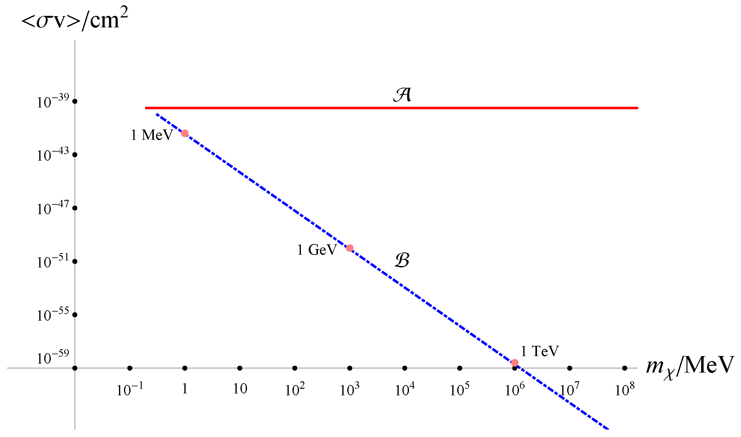
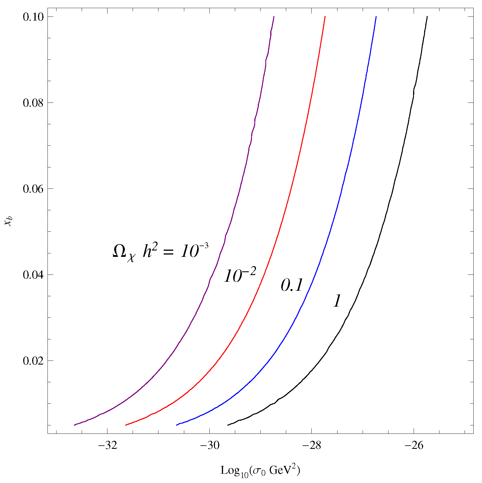
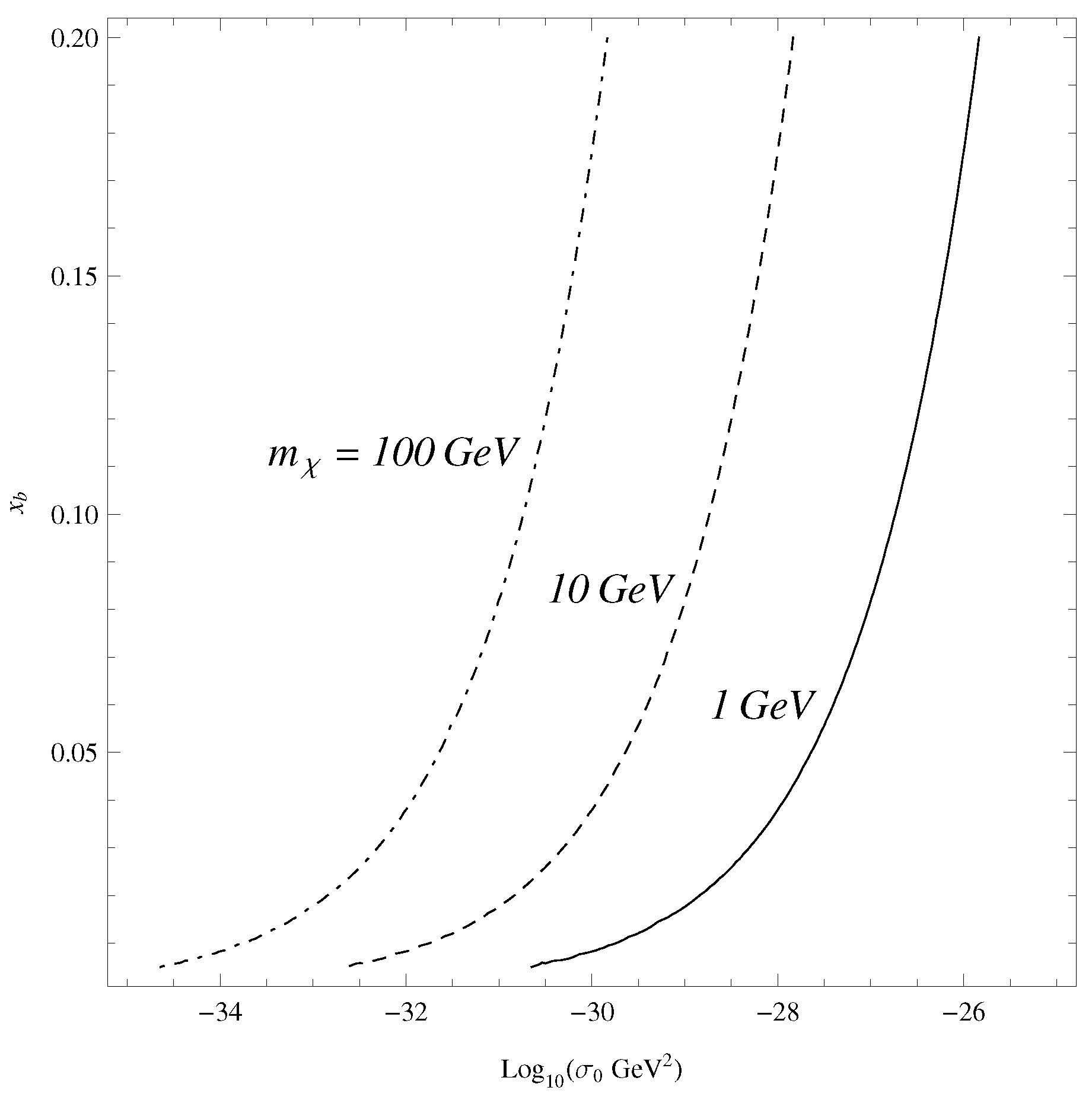
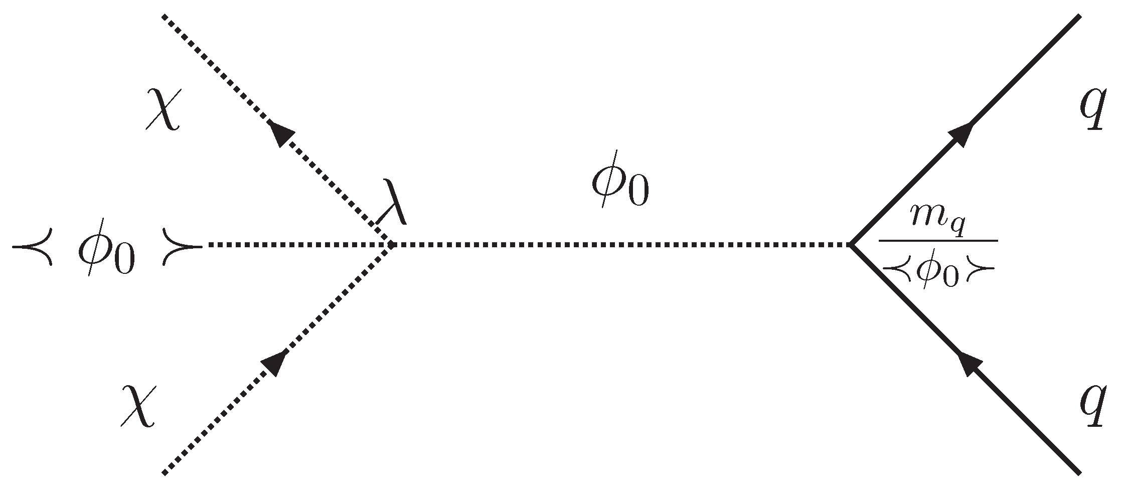
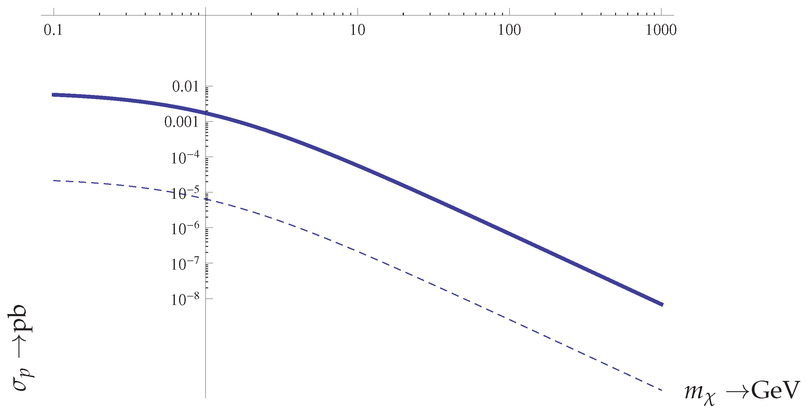
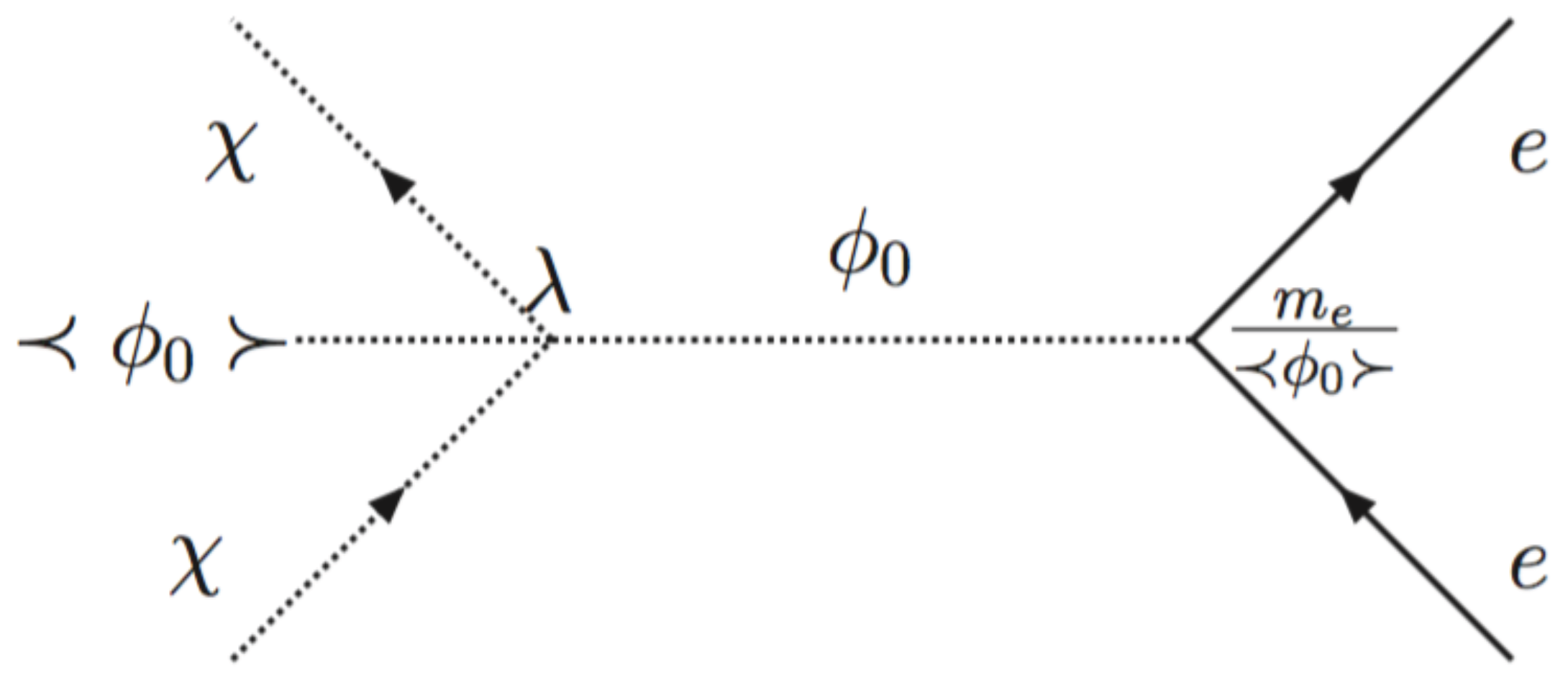
4. Direct Detections of Dark Matter to Test the Big Bounce Genesis

In order to unravel the nature of DM, it is essential to directly detect it. The possibility of such direct detection, of course, depends on the nature of the DM constituents and their interactions. For the extremely non-relativistic DM candidates, such as WIMP and most species of DM candidates in BBG, their average kinetic energy today is too low to excite the nucleus. Therefore, they can be directly detected mainly via the recoiling of a nucleus $(A,Z)$ in elastic scattering. The event rate for such a process is mainly determined with the following three ingredients [84]:

• The elementary DM-nucleon cross-section computed in quantum field theory;
• The knowledge of the relevant nuclear matrix elements obtained with as reliable as possible many body nuclear wave functions;
• The knowledge of the density of DM in our vicinity and its velocity distribution;

where the last two ingredients have been discussed extensively in [61], but we are not going to discuss these two ingredients in this work further.

For the purpose of comparing the predictions of BBG with direct DM search [85,86,87,88,89,90,91,92,93,94,95,96], we focus on the study of the DM-nucleon cross-section in this section following [61,64].

Cosmologically, the characteristic relation of the thermally-averaged cross-section $\langle \sigma v\rangle$ and $m_{\chi }$, such as Equation (8), has been obtained for the case of the scalar DM particles χ interacting with another scalar ϕ via a quartic coupling. However, this relation cannot be utilized directly for comparing with the results of direct detection, because $\langle \sigma v\rangle$ is, essentially, the cross-section of the DM pair-annihilation, but not the DM-nucleon cross-section, ${\sigma }_p$, measured in direct detection experiments [85,86,87,88,89,90,91,92,93,94,95,96].

The elementary DM-nucleon cross-section, ${\sigma }_p$, can be computed with the Feynman diagram (Figure 7), in which the scalar DM particle interacts with the quark mediated by ϕ [61].

The resulting DM-nucleon cross-section is given by [61]:

$${\sigma }_p=\frac{1}{4\pi }\frac{{\lambda }^2{m}_p^2\left({\mu }_r^2\right)}{m_{\varphi }^4}\frac{1}{m_{\chi }^2}{(\sum _q{f}_q)}^2=\frac{1}{4\pi }\frac{{\lambda }^2{m}_p^2}{m_{\varphi }^4}\frac{1}{{\left(1+m_{\chi }/m_p\right)}^2}{(\sum _q{f}_q)}^2$$

(45)

where $m_p$, $m_{\varphi }$ and $m_{\chi }$ are, respectively, the mass of proton, ϕ and χ. ${\mu }_r$ is the DM-nucleus reduced mass, and $f_q$ is related to the probability of finding the quark q in the nucleon.

Note that the vacuum expectation value $\prec {\varphi }_0\succ$ in the quartic coupling is cancelled by the Yukawa coupling of scalar ϕ with the quarks. Therefore, the elementary DM-nucleon cross-section, ${\sigma }_p$, can be fully determined with a set of parameters, $(m_{\chi },m_{\varphi },\lambda )$. If the quartic coupling of the scalar DM with the Higgs is the same with the usual quartic coupling of the Higgs particle discovered at the LHC, $\lambda =1/2$, $m_{\varphi }=126$ GeV, one finds:

$${\sigma }_p={\sigma }_0{\left(1+\frac{m_{\chi }}{m_p}\right)}^{-2},{\sigma }_0=6\times {10}^{-11}{m}_p^{-2}{\left(\sum _q{f}_q\right)}^2$$

(46)

The value of ${\sum }_q{f}_q$, of course, can vary a great deal [97,98,99,100,101,102,103], but its value has now become very much constrained by lattice experiments [104], yielding ${\sum }_q{f}_q=0.2$, which we will adopt in this work. Thus, we get ${\sigma }_0=0.8\times {10}^{-3}$ pb, which is a bit high leading to ${\sigma }_p=2.7\times {10}^{-6}$ pb at $m_{\chi }=$ 50 GeV compared to the limit of $\times {10}^{-8}$ pb extracted by the Xe experiments XENON100 [86,87]. We can, of course, treat the quartic Higgs coupling λ as a phenomenological parameter and adjust so that it yields ${\sigma }_0=2.6\times {10}^{-5}$ pb, yielding the value ${\sigma }_p=1.0\times {10}^{-8}$ pb, and makes our model consistent with the limit extracted from experiments, e.g., XENON100 [86,87] for heavy DM candidates, $m_{\chi }=$ 50 GeV. The thus-obtained nucleon cross-sections are exhibited in Figure 8. Our model, however, yields the value of ${\sigma }_0=0.6\times {10}^{-4}$ pb for $m_{\chi }=$ 10 GeV, consistent with the the recent low threshold CRESST experiment [94], which is perhaps more suitable for low mass DM favoured by our model.

We should stress that the DM nucleon cross-section dependence exhibited in the exclusion plots is purely kinematic, and it does not contain any actual dependence on the cross-section of the elementary nucleon cross-section as in our model. The extra mass dependence of the cross-section of scalar DM, exhibiting an enhancement in the low DM mass regime, may favour the searches at low energy transfers. It is interesting to compare the behaviour of this cross-section with that of the relic abundance of the BBG shown in Figure 2.

At the end, we also notice another interesting domain of this BBG model in which the DM candidate is light. One can find that such a DM with a mass less than 100 MeV cannot produce a detectable recoiling nucleus, but it could produce electrons [105] with energies in the tens of eV, which could be detected with current mixed phase detectors [106]. If the DM is a scalar particle, however, it can interact in a similar pattern with other fermions, e.g., electrons. The relevant Feynman diagram is shown in Figure 9.

For a DM with a mass in the range of the electron mass, both the DM particle and the electron are not relativistic. Therefore, the expression for the elementary electron cross-section is similar to that of hadrons, i.e., it is now given by:

$${\sigma }_e=\frac{1}{4\pi }\frac{{\lambda }^2{m}_e^2}{m_{\varphi }^4}{\left(\frac{m_e{m}_{\chi }}{m_e+m_{\chi }}\right)}^2\frac{1}{m_{\chi }^2}$$

(47)

This is a respectably-sized cross-section dependent on the ratio $m_{\chi }/m_e$. In this case, one must consider electron recoils, but the highest possible electron energy is about 1.5 eV, and the DM mass must greater than 0.3 electron masses. Therefore, the detection of a DM with a mass around the electron mass requires another type of detector [61,64].

5. Summary

In this review, we discuss the Big Bounce Genesis (BBG) as a unified framework for the interplay between dark matter (DM) and the early evolution of the universe, particularly, in which the famous WIMP and WIMP-less miracles are also included. The novelty of BBG is that it provides a new possibility of using DM mass and its predicted interaction cross-section, as a telling signal of the existence of a big bounce at the early stage in the evolution of our currently-observed universe. Each type of BBG model, bosonic/fermionic DM in a high/low temperature bounce, and its predictions have been discussed in detail. These predictions can be checked against data from the present and future DM searches.

Another salient feature of BBG is that out-of-chemical equilibrium production is allowed. In this case, the abundance of DM is much less than its thermal equilibrium value; the thermal fluctuation of DM, then, can be generated; in sharp contrast to the case in which thermal fluctuations are suppressed in the thermal equilibrium production. In this review, we also present a detailed and model-independent analysis of the whole evolution of DM thermal fluctuations in a generic bounce. It may have important implications on the formation of large-scale structures, clusters, galaxies and primordial black holes and potentially can be compared with astrophysical observations.

At the end of this review, we also presented a detailed analysis of the predicted event rates for different DM detection experiments: events/kg/year for nuclear recoil experiments for heavy scalar DM in the mass range of 100 GeV and the event rate for MeV light scalar DM detections by electronic scattering.

References

1. Laozi. 14th Chapter of Tao Te Ching; China Book Company: Beijing, China, 2015. [Google Scholar]
2. Guth, A.H. The Inflationary Universe: A Possible Solution to the Horizon and Flatness Problems. Phys. Rev. 1981, D23, 347–356. [Google Scholar] [CrossRef]
3. Weiland, J.L.; Odegard, N.; Hill, R.S.; Wollack, E.; Hinshaw, G.; Greason, M.R.; Jarosik, N.; Page, L.; Bennett, C.L.; Dunkley, J.; et al. Seven-Year Wilkinson Microwave Anisotropy Probe (WMAP) Observations: Cosmological Interpretation. Astrophys. J. Suppl. 2011, 192, 18. [Google Scholar] [CrossRef]
4. Ade, P.A.R.; Aghanim, N.; Armitage-Caplan, C.; Arnaud, M.; Ashdown, M.; Atrio-Barandela, F.; Aumont, J.; Baccigalupi, C.; Banday, A.J.; Barreiro, R.B.; et al. Planck 2013 results. XV. CMB power spectra and likelihood. Astron. Astrophys. 2014, 571, A15. [Google Scholar]
5. Mukhanov, V.F.; Feldman, H.; Brandenberger, R.H. Theory of cosmological perturbations. Part 1. Classical perturbations. Part 2. Quantum theory of perturbations. Part 3. Extensions. Phys. Rep. 1992, 215, 203–333. [Google Scholar] [CrossRef]
6. Borde, A.; Vilenkin, A. Eternal inflation and the initial singularity. Phys. Rev. Lett. 1994, 72, 3305–3309. [Google Scholar] [CrossRef] [PubMed]
7. Novello, M.; Bergliaffa, A.E.P. Bouncing Cosmologies. Phys. Rep. 2008, 463, 127. [Google Scholar] [CrossRef]
8. Brandenberger, R.H. The Matter Bounce Alternative to Inflationary Cosmology. arXiv:1206.4196 [astro-ph.CO].
9. Battefeld, D.; Peter, P. A Critical Review of Classical Bouncing Cosmologies. Phys. Rep. 2015, 571, 1–66. [Google Scholar] [CrossRef]
10. Brandenberger, R.; Peter, P. Bouncing Cosmologies: Progress and Problems. arXiv, 2016; [arXiv:hep-th/1603.05834]. [Google Scholar]
11. Khoury, J.; Ovrut, B.A.; Steinhardt, P.J.; Turok, N. The Ekpyrotic universe: Colliding branes and the origin of the hot big bang. Phys. Rev. 2001, D64, 123522. [Google Scholar] [CrossRef]
12. Steinhardt, P.J.; Turok, N. Cosmic evolution in a cyclic universe. Phys. Rev. 2002, D65, 126003. [Google Scholar] [CrossRef]
13. Steinhardt, P.J.; Turok, N. A cyclic model of the universe. Science 2002, 296, 1436–1439. [Google Scholar] [CrossRef] [PubMed]
14. Gasperini, M.; Veneziano, G. The Pre-big bang scenario in string cosmology. Phys. Rep. 2003, 373, 1–212. [Google Scholar] [CrossRef]
15. Creminelli, P.; Luty, M.A.; Nicolis, A.; Senatore, L. Starting the Universe: Stable Violation of the Null Energy Condition and Non-standard Cosmologies. JHEP 2006, 2006, 080. [Google Scholar] [CrossRef]
16. Cai, Y.F.; Qiu, T.; Piao, Y.S.; Li, M.; Zhang, X. Bouncing universe with quintom matter. JHEP 2007, 2007, 071. [Google Scholar] [CrossRef]
17. Cai, Y.F.; Qiu, T.; Brandenberger, R.; Zhang, X. A Nonsingular Cosmology with a Scale-Invariant Spectrum of Cosmological Perturbations from Lee-Wick Theory. Phys. Rev. 2009, D80, 023511. [Google Scholar] [CrossRef]
18. Wands, D. Cosmological perturbations through the big bang. Adv. Sci. Lett. 2009, 2, 194–204. [Google Scholar] [CrossRef]
19. Bhattacharya, K.; Cai, Y.F.; Das, S. Lee-Wick radiation induced bouncing universe models. Phys. Rev. 2013, D87, 083511. [Google Scholar] [CrossRef]
20. Odintsov, S.D.; Oikonomou, V.K. Matter Bounce Loop Quantum Cosmology from F(R) Gravity. Phys. Rev. 2014, D90, 124083. [Google Scholar]
21. Li, H.; Li, M.; Qiu, T.; Xia, J.; Piao, Y.; Zhang, X. What can we learn from the tension between PLANCK and BICEP2 data? Sci. China Phys. Mech. Astron. 2014, 57, 1431–1441. [Google Scholar] [CrossRef]
22. Quintin, J.; Cai, Y.F.; Brandenberger, R.H. Matter Creation in a Nonsingular Bouncing Cosmology. Phys. Rev. D 2014, 90, 063507. [Google Scholar] [CrossRef]
23. Wan, Y.; Li, S.; Li, M.; Qiu, T.; Cai, Y.; Zhang, X. Single field inflation with modulated potential in light of the Planck and BICEP2. Phys. Rev. D 2014, 90, 023537. [Google Scholar] [CrossRef]
24. Cai, Y.F. Exploring Bouncing Cosmologies with Cosmological Surveys. Sci. China Phys. Mech. Astron. 2014, 57, 1414–1430. [Google Scholar] [CrossRef]
25. Liu, Z.G.; Li, H.; Piao, Y.S. Pre-inflationary genesis with CMB B-mode polarization. Phys. Rev. D 2014, 90, 083521. [Google Scholar] [CrossRef]
26. Li, M. Generating scale-invariant tensor perturbations in the non-inflationary universe. Phys. Lett. B 2014, 736, 488–493. [Google Scholar] [CrossRef]
27. Cai, Y.F.; Wang, Y. Testing quantum gravity effects with latest CMB observations. Phys. Lett. 2014, B735, 108–111. [Google Scholar] [CrossRef]
28. Cai, Y.F.; Quintin, J.; Saridakis, E.N.; Wilson-Ewing, E. Nonsingular bouncing cosmologies in light of BICEP2. J. Cosmol. Astropart. Phys. 2014, 2014, 033. [Google Scholar] [CrossRef]
29. Hu, B.; Hu, J.W.; Guo, Z.K.; Cai, R.G. Reconstruction of the primordial power spectra with Planck and BICEP2. Phys. Rev. D 2014, 90, 023544. [Google Scholar] [CrossRef]
30. Li, H.; Xia, J.Q.; Zhang, X. Global fitting analysis on cosmological models after BICEP2. arXiv, 2014; [arXiv:astro-ph.CO/1404.0238]. [Google Scholar]
31. Xia, J.Q.; Cai, Y.F.; Li, H.; Zhang, X. Evidence for bouncing evolution before inflation after BICEP2. Phys. Rev. Lett. 2014, 112, 251301. [Google Scholar] [CrossRef] [PubMed]
32. Nojiri, S.; Odintsov, S.D.; Oikonomou, V.K. Unimodular F(R) Gravity. JCAP 2016, 1605, 046. [Google Scholar] [CrossRef]
33. Nojiri, S.; Odintsov, S.D.; Oikonomou, V.K. Bounce universe history from unimodular F(R) gravity. Phys. Rev. 2016, D93, 084050. [Google Scholar]
34. Cheung, Y.K.E.; Song, X.; Li, S.; Li, Y.; Zhu, Y. A smoothly bouncing universe from String Theory. arXiv, 2016; [arXiv:gr-qc/1601.03807]. [Google Scholar]
35. Escofet, A.; Elizalde, E. Gauss–Bonnet modified gravity models with bouncing behaviour. Mod. Phys. Lett. 2016, A31, 1650108. [Google Scholar] [CrossRef]
36. Haro, J.; Makarenko, A.N.; Myagky, A.N.; Odintsov, S.D.; Oikonomou, V.K. Bouncing loop quantum cosmology in Gauss-Bonnet gravity. Phys. Rev. 2015, D92, 124026. [Google Scholar] [CrossRef]
37. Odintsov, S.D.; Oikonomou, V.K. Deformed Matter Bounce with Dark Energy Epoch. Phys. Rev. D 2016, 94, 064022. [Google Scholar] [CrossRef]
38. Choudhury, S.; Banerjee, S. Hysteresis in the Sky. Astropart. Phys. 2016, 80, 34–89. [Google Scholar] [CrossRef]
39. Odintsov, S.D.; Oikonomou, V.K. Big-Bounce with Finite-time Singularity: The F(R) Gravity Description. arXiv, 2015; [arXiv:gr-qc/1512.04787]. [Google Scholar]
40. Oikonomou, V.K. Singular Bouncing Cosmology from Gauss-Bonnet Modified Gravity. Phys. Rev. 2015, D92, 124027. [Google Scholar] [CrossRef]
41. Cai, Y.F.; Wilson-Ewing, E. A ΛCDM bounce scenario. JCAP 2015, 1503, 006. [Google Scholar] [CrossRef] [PubMed]
42. Cai, Y.F.; Duplessis, F.; Easson, D.A.; Wang, D.G. Searching for a matter bounce cosmology with low redshift observations. Phys. Rev. 2016, D93, 043546. [Google Scholar] [CrossRef]
43. Ferreira, E.G.M.; Brandenberger, R. Holographic Curvature Perturbations in a Cosmology with a Space-Like Singularity. JCAP 2016, 1607, 030. [Google Scholar] [CrossRef]
44. Quintin, J.; Sherkatghanad, Z.; Cai, Y.F.; Brandenberger, R.H. Evolution of cosmological perturbations and the production of non-Gaussianities through a nonsingular bounce: Indications for a no-go theorem in single field matter bounce cosmologies. Phys. Rev. 2015, D92, 063532. [Google Scholar] [CrossRef]
45. Brandenberger, R.H.; Cai, Y.F.; Das, S.R.; Ferreira, E.G.M.; Morrison, I.A.; Wang, Y. Fluctuations in a Cosmology with a Space-Like Singularity and their Gauge Theory Dual Description. arXiv, 2016; [arXiv:hep-th/1601.00231]. [Google Scholar]
46. Hipolito-Ricaldi, W.S.; Brandenberger, R.; Ferreira, E.G.M.; Graef, L.L. Particle Production in Ekpyrotic Scenarios. arXiv, 2016; [arXiv:hep-th/1605.04670]. [Google Scholar]
47. Wan, Y.; Qiu, T.; Huang, F.P.; Cai, Y.F.; Li, H.; Zhang, X. Bounce Inflation Cosmology with Standard Model Higgs Boson. JCAP 2015, 1512, 019. [Google Scholar] [CrossRef]
48. Cai, Y.F.; Wilson-Ewing, E. Non-singular bounce scenarios in loop quantum cosmology and the effective field description. JCAP 2014, 1403, 026. [Google Scholar] [CrossRef]
49. Wands, D. Duality invariance of cosmological perturbation spectra. Phys. Rev. 1999, D60, 023507. [Google Scholar] [CrossRef]
50. Finelli, F.; Brandenberger, R. On the generation of a scale invariant spectrum of adiabatic fluctuations in cosmological models with a contracting phase. Phys. Rev. 2002, D65, 103522. [Google Scholar] [CrossRef]
51. Li, C.; Cheung, Y.K.E. The scale invariant power spectrum of the primordial curvature perturbations from the coupled scalar tachyon bounce cosmos. JCAP 2014, 1407, 008. [Google Scholar] [CrossRef] [PubMed]
52. Li, C.; Wang, L.; Cheung, Y.K.E. Bound to bounce: A coupled scalar?tachyon model for a smooth bouncing/cyclic universe. Phys. Dark Univ. 2014, 3, 18–33. [Google Scholar] [CrossRef]
53. Li, C. Thermally producing and weakly freezing out dark matter in a bouncing universe. Phys. Rev. 2015, D92, 063513. [Google Scholar] [CrossRef]
54. Boyle, L.A.; Steinhardt, P.J.; Turok, N. A New duality relating density perturbations in expanding and contracting Friedmann cosmologies. Phys. Rev. 2004, D70, 023504. [Google Scholar] [CrossRef]
55. Li, C.; Cheung, Y.K.E. Dualities between Scale Invariant and Magnitude Invariant Perturbation Spectra in Inflationary/Bouncing Cosmos. arXiv, 2012; [arXiv:gr-qc/1211.1610]. [Google Scholar]
56. Li, C.; Brandenberger, R.H.; Cheung, Y.K.E. Big Bounce Genesis. Phys. Rev. 2014, D90, 123535. [Google Scholar] [CrossRef]
57. Scherrer, R.J.; Turner, M.S. On the Relic, Cosmic Abundance of Stable Weakly Interacting Massive Particles. Phys. Rev. 1986, D33, 1585. [Google Scholar]
58. Feng, J.L.; Kumar, J. The WIMPless Miracle: Dark-Matter Particles without Weak-Scale Masses or Weak Interactions. Phys. Rev. Lett. 2008, 101, 231301. [Google Scholar] [CrossRef] [PubMed]
59. Kolb, E.W.; Turner, M.S. The Early Universe. Front. Phys. 1990, 69, 1–547. [Google Scholar]
60. Gondolo, P.; Gelmini, G. Cosmic abundances of stable particles: Improved analysis. Nucl. Phys. 1991, B360, 145–179. [Google Scholar] [CrossRef]
61. Cheung, Y.K.E.; Vergados, J.D. Direct dark matter searches—Test of the Big Bounce Cosmology. JCAP 2015, 1502, 014. [Google Scholar] [CrossRef]
62. Cheung, Y.K.E.; Kang, J.U.; Li, C. Dark matter in a bouncing universe. JCAP 2014, 1411, 001. [Google Scholar] [CrossRef] [PubMed]
63. Cai, Y.F.; Brandenberger, R.; Zhang, X. Preheating a bouncing universe. Phys. Lett. 2011, B703, 25–33. [Google Scholar] [CrossRef]
64. Vergados, J.D.; Moustakidis, C.C.; Cheung, Y.K.E.; Ejri, H.; Kim, Y.; Lie, Y. Light WIMP searches involving electron scattering. arXiv, 2016; [arXiv:hep-ph/1605.05413]. [Google Scholar]
65. Li, C. Thermal Fluctuations of Dark Matter in Bouncing Cosmology. JCAP 2016, 1609, 038. [Google Scholar] [CrossRef]
66. Peskin, M.E.; Schroeder, D.V. An Introduction to Quantum Field Theory; Addison-Wesley: New York, NY, USA, 1995. [Google Scholar]
67. Capozziello, S.; Francaviglia, M. Extended Theories of Gravity and their Cosmological and Astrophysical Applications. Gen. Rel. Grav. 2008, 40, 357–420. [Google Scholar] [CrossRef]
68. Capozziello, S.; De Laurentis, M. The dark matter problem from f(R) gravity viewpoint. Ann. Phys. 2012, 524, 545–578. [Google Scholar] [CrossRef]
69. Qiu, T.; Evslin, J.; Cai, Y.F.; Li, M.; Zhang, X. Bouncing Galileon Cosmologies. JCAP 2011, 1110, 036. [Google Scholar] [CrossRef]
70. Qiu, T.; Gao, X.; Saridakis, E.N. Towards anisotropy-free and nonsingular bounce cosmology with scale-invariant perturbations. Phys. Rev. D 2013, 88, 043525. [Google Scholar] [CrossRef]
71. Qiu, T.; Wang, Y.T. G-Bounce Inflation: Towards Nonsingular Inflation Cosmology with Galileon Field. JHEP 2015, 1504, 130. [Google Scholar] [CrossRef]
72. Chung, D.J.; Kolb, E.W.; Riotto, A. Nonthermal supermassive dark matter. Phys. Rev. Lett. 1998, 81, 4048–4051. [Google Scholar] [CrossRef]
73. Cai, Y.F.; Xue, W.; Brandenberger, R.; Zhang, X. Thermal Fluctuations and Bouncing Cosmologies. JCAP 2009, 0906, 037. [Google Scholar] [CrossRef]
74. Biswas, T.; Brandenberger, R.; Koivisto, T.; Mazumdar, A. Cosmological perturbations from statistical thermal fluctuations. Phys. Rev. 2013, D88, 023517. [Google Scholar] [CrossRef]
75. Navarro, J.F.; Frenk, C.S.; White, S.D.M. The Structure of cold dark matter halos. Astrophys. J. 1996, 462, 563–575. [Google Scholar] [CrossRef]
76. Zhao, D.; Mo, H.; Jing, Y.; Boerner, G. The growth and structure of dark matter haloes. Mon. Not. R. Astron. Soc. 2003, 339, 12–24. [Google Scholar] [CrossRef]
77. Diemand, J.; Moore, B.; Stadel, J. Earth-mass dark-matter haloes as the first structures in the early Universe. Nature 2005, 433, 389–391. [Google Scholar] [CrossRef] [PubMed]
78. Frenk, C.S.; White, S.D.M. Dark matter and cosmic structure. Ann. Phys. 2012, 524, 507–534. [Google Scholar] [CrossRef]
79. Bromm, V.; Yoshida, N.; Hernquist, L.; McKee, C.F. The formation of the first stars and galaxies. Nature 2009, 459, 49–54. [Google Scholar] [CrossRef] [PubMed]
80. Umeda, H.; Yoshida, N.; Nomoto, K.; Tsuruta, S.; Sasaki, M.; Ohkubo, T. Early Black Hole Formation by Accretion of Gas and Dark Matter. JCAP 2009, 0908, 024. [Google Scholar] [CrossRef]
81. Colberg, J.M.; White, S.D.M.; Yoshida, N.; MacFarland, T.J.; Jenkins, A.; Frenk, C.S.; Pearce, F.R.; Evrard, A.E.; Couchman, H.M.P.; Efstathiou, G.; et al. Clustering of galaxy clusters in CDM universes. Mon. Not. R. Astron. Soc. 2000, 319, 209. [Google Scholar] [CrossRef]
82. Di Matteo, T.; Croft, R.A.C.; Springel, V.; Hernquist, L. Black hole growth and activity in a lambda CDM universe. Astrophys. J. 2003, 593, 56–68. [Google Scholar] [CrossRef]
83. Maccio, A.V.; Ruchayskiy, O.; Boyarsky, A.; Munoz-Cuartas, J.C. The inner structure of haloes in Cold+Warm dark matter models. Mon. Not. R. Astron. Soc. 2013, 428, 882–890. [Google Scholar] [CrossRef]
84. Lewin, J.D.; Smith, P.F. Review of mathematics, numerical factors, and corrections for dark matter experiments based on elastic nuclear recoil. Astropart. Phys. 1996, 6, 87–112. [Google Scholar] [CrossRef]
85. Angle, J.; Aprile, E.; Arneodo, F.; Baudis, L.; Bernstein, A.; Bolozdynya, A.I.; Coelho, L.C.C.; Dahl, C.E.; DeViveiros, L.; Ferella, A.D.; et al. Search for Light Dark Matter in XENON10 Data. Phys. Rev. Lett. 2011, 107, 051301, Erratum: Phys. Rev. Lett. 2013, 110, 249901. [Google Scholar] [CrossRef] [PubMed] [Green Version]
86. Aprile, E.; Arisaka, K.; Arneodo, F.; Askin, A.; Baudis, L.; Behrens, A.; Bokeloh, K.; Brown, E.; Bruch, T.; Bruno, G.; et al. Dark matter results from 100 live days of XENON100 data. Phys. Rev. Lett. 2011, 107, 131302. [Google Scholar] [CrossRef] [PubMed]
87. Aprile, E.; Alfonsi, M.; Arisaka, K.; Arneodo, F.; Balan, C.; Baudis, L.; Bauermeister, B.; Behrens, A.; Beltrame, P.; Bokeloh, K.; et al. Dark matter results from 225 live days of XENON100 data. Phys. Rev. Lett. 2011, 109, 181301. [Google Scholar] [CrossRef] [PubMed]
88. Aalseth, C.E.; Barbeau, P.S.; Bowden, N.S.; Cabrera-Palmer, B.; Colaresi, J.; Collar, J.I.; Dazeley, S.; de Lurgio, P.; Fast, J.E.; Fields, V.; et al. Results from a search for light-mass dark matter with a p-type point contact germanium detector. Phys. Rev. Lett. 2011, 106, 131301. [Google Scholar] [CrossRef] [PubMed]
89. Bernabei, R.; Belli, P.; Cappella, F.; Cerulli, R.; Dai, C.J.; d’Angelo, A.; He, H.L.; IncicchittiH, A.; Kuang, H.H.; Ma, J.M.; et al. First results from DAMA/LIBRA and the combined results with DAMA/NaI. Eur. Phys. J. C 2008, 56, 333–355. [Google Scholar] [CrossRef]
90. Belli, P.; Bernabei, R.; Bottino, A.; Cappella, F.; Cerulli, R.; Fornengo, N.; Scopel, S. Observations of annual modulation in direct detection of relic particles and light neutralinos. Phys. Rev. D 2011, 84, 055014. [Google Scholar] [CrossRef] [Green Version]
91. Malling, D.C.; Akerib, D.S.; Araujo, H.M.; Bai, X.; Bedikian, S.; Bernard, E.; Bernstein, A.; Bradley, A.; Cahn, S.B.; Carmona-Benitez, M.C.; et al. After LUX: The LZ program. arXiv:1110.0103 [astro-ph.IM].
92. Akerib, D.S.; Alvaro-Dean, J.; Armel-Funkhouser, M.S.; Attisha, M.J.; Baudis, L.; Bauer, D.; Beaty, A.J.; Brink, P.L.; Bunker, R.; Burke, S.P.; et al. First results from the cryogenic dark matter search in the soudan underground laboratory. Phys. Rev. Lett. 2004, 93, 211301. [Google Scholar] [CrossRef] [PubMed]
93. Di Stefano, P.; Bruckmayer, M.; Buccic, C.; Cooper, S.; Cozzini, C.; von Feilitzschd, F.; Frank, T.; Hauff, D.; Jagemann, T.; Jochum, J.; et al. The CRESST experiment: Recent results and prospects. In Proceedings of the Cosmology and Particle Physics: CAPP 2000, Verbier, Switzerland, 17–28 July 2000; Volume 555, p. 381. [CrossRef]
94. Angloher, G.; Bento, A.; Bucci, C.; Canonica, L.; Defay, X.; Erb, A.; von Feilitzsch, F.; Ferreiro Iachellini, N.; Gorla, P.; Gütlein, A.; et al. Results on light dark matter particles with a low-threshold CRESST-II detector. Eur. Phys. J. C 2016, 76, 1–8. [Google Scholar] [CrossRef]
95. Archambault, S.; Aubin, F.; Auger, M.; Behnke, E.; Beltran, B.; Clark, K.; Daib, X.; Davourb, A.; Farined, J.; Faust, R.; et al. Dark matter spin-dependent limits for WIMP interactions on 19F by PICASSO. Phys. Lett. B 2009, 682, 185–192. [Google Scholar] [CrossRef]
96. Archambault, S.; Aubin, F.; Auger, M.; Beleshi, M.; Behnke, E.; Behnke, J.; Beltran, B.; Clark, K.; Dai, X.; Das, M.; et al. New insights into particle detection with superheated liquids. New J. Phys. 2011, 13, 043006. [Google Scholar] [CrossRef]
97. Cheng, T.P. Chiral Symmetry and the Higgs Nucleon Coupling. Phys. Rev. D 1988, 38, 2869. [Google Scholar] [CrossRef]
98. Cheng, H.Y. Low-energy Interactions of Scalar and Pseudoscalar Higgs Bosons With Baryons. Phys. Lett. B 1989, 219, 347–353. [Google Scholar] [CrossRef]
99. Djouadi, A.; Drees, M. QCD corrections to neutralino nucleon scattering. Phys. Lett. B 2000, 484, 183–191. [Google Scholar] [CrossRef]
100. Dawson, S. Radiative corrections to Higgs boson production. Nucl. Phys. B 1991, 359, 283–300. [Google Scholar] [CrossRef]
101. Spira, M.; Djouadi, A.; Graudenz, D.; Zerwas, P.M. Higgs boson production at the LHC. Nucl. Phys. B 1995, 453, 17–82. [Google Scholar] [CrossRef]
102. Ellis, J.R.; Ferstl, A.; Olive, K.A. Reevaluation of the elastic scattering of supersymmetric dark matter. Phys. Lett. B 2000, 481, 304–314. [Google Scholar] [CrossRef]
103. Vergados, J.D. On the direct detection of dark matter- exploring all the signatures of the neutralino-nucleus interaction. Lect. Notes Phys. 2007, 720, 69. [Google Scholar]
104. Giedt, J.; Thomas, A.W.; Young, R.D. Dark matter, the CMSSM and lattice QCD. Phys. Rev. Lett. 2009, 103, 201802. [Google Scholar] [CrossRef] [PubMed]
105. Moustakidis, C.C.; Vergados, J.D.; Ejiri, H. Direct dark matter detection by observing electrons produced in neutralino-nucleus collisions. Nucl. Phys. B 2005, 727, 406. [Google Scholar] [CrossRef]
106. Aprile, E.; Alfonsi, M.; Arisaka, K.; Arneodo, F.; Balan, C.; Baudis, L.; Bauermeister, B.; Behrens, A.; Beltrame, P.; Bokeloh, K.; et al. Observation and applications of single-electron charge signals in the XENON100 experiment. J. Phys. G 2014, 41, 035201. [Google Scholar] [CrossRef]
Figure 1. The exit and entrance of physical perturbations at the Hubble horizon in the inflation (left) and in the bounce (right) scenarios.
Symmetry 08 00136 g001
Figure 2. The cross-section σ υ as a function of the scalar dark matter (DM) mass. In the standard cosmology, it is a constant (solid line), but it varies considerably in the bounce universe scenario (dash-dotted line) [56].
Symmetry 08 00136 g002
Figure 3. The breakdown of the Big Bounce period into a pre-bounce contraction (Phase I), a post-bounce expansion (Phase II) and the freeze-out of the DM particles (Phase III).
Symmetry 08 00136 g003
Figure 4. A schematic plot of the time evolution of DM in a generic bounce universe scenario. Two pathways of producing DM yet satisfying current observations’ thermal production (which is indistinguishable from standard cosmology) and non-thermal production (characteristic of the bounce universe) are illustrated. The horizontal axis indicates both the time, t, as well as the temperature, T, of the cosmological background [56].
Symmetry 08 00136 g004
Figure 5. Contour plots of the predicted relic abundance in the ( x b - σ ˜ 0 ) plane in the high temperature bounce case. Here, we take m χ = 1 GeV [62].
Symmetry 08 00136 g005
Figure 6. Low temperature bounce: x b as a function of a to reproduce the present relic abundance Ω χ h 2 0 . 1 for various m χ [62].
Symmetry 08 00136 g006
Figure 7. The quark-scalar DM scattering mediated by a scalar particle [61].
Symmetry 08 00136 g007
Figure 8. The nucleon cross-section as a function of the DM mass in the case of a scalar DM particle: as predicted by our model (thick solid line), consistent with the low DM mass CRESSTII experiment [94] and with the quartic coupling λ adjusted to fit the limit of the Xe100 experiment, for a DM mass of 50 GeV, i.e., σ p = 10 8 pb (dashed line).
Symmetry 08 00136 g008
Figure 9. The quark-scalar dark matter scattering mediated by a scalar particle [61].
Symmetry 08 00136 g009