Energy Conservation Law in Industrial Architecture: An Approach through Geometric Algebra

Abstract

Since 1892, the electrical engineering scientific community has been seeking a power theory for interpreting the power flow within electric networks under non-sinusoidal conditions. Although many power theories have been proposed regarding non-sinusoidal operation, an adequate solution is yet to be found. Using the framework based on complex algebra in non-sinusoidal circuit analysis (frequency domain), the verification of the energy conservation law is only possible in sinusoidal situations. In this case, reactive energy turns out to be proportional to the energy difference between the average electric and magnetic energies stored in the loads and its cancellation is mathematically trivial. However, in industrial architecture, apparent power definition of electric loads (non-sinusoidal conditions) is inconsistent with the energy conservation law. Up until now, in the classical complex algebra approach, this goal is only valid in the case of purely resistive loads. Thus, in this paper, a new circuit analysis approach using geometric algebra is used to develop the most general proof of energy conservation in industrial building loads. In terms of geometric objects, this powerful tool calculates the voltage, current, and apparent power in electrical systems in non-sinusoidal, linear/nonlinear situations. In contrast to the traditional method developed by Steinmetz, the suggested powerful tool extends the concept of phasor to multivector-phasors and is performed in a new Generalized Complex Geometric Algebra structure (CGn), where Gn is the Clifford algebra in n-dimensional real space and C is the complex vector space. To conclude, a numerical example illustrates the clear advantages of the approach suggested in this paper.

1. Introduction

Most of the harmonic problems affecting electrical distribution networks in industrial architecture are generated within the building. This is partly due to the proliferation of linear and nonlinear loads connected to the circuits in the building; air conditioning, computers, CCTV, servers, adjustable speed drive (ASD), and other electronic equipment, are the main sources of problems. The result of using such a high number of nonlinear loads is that the current waveform is distorted, causing excessive harmonic voltages to be generated. Also, the close proximity of many of these buildings with similar industrial activities will definitely contribute to the distortion of the electric power quality of feed supplying these constructions. These harmonics can cause serious problems in power systems, for example, excessive heat in appliances, premature aging of electrical equipment, derating of equipment, fault of protection, and lower power factor. Consequently, harmonic energy losses reduce the efficiency of power systems and cause significant costs in distribution networks. The disadvantages of harmonics have been discussed extensively, including such factors as the cost effect [1,2].

The challenge of developing a power theory suitable for harmonic analysis has continued over last century. Since the appearance of the first power theory developed by Budeanu in 1927, significant research efforts [3,4,5,6,7,8,9,10,11] have been made to find out a valid definition of the apparent power in n-sinusoidal situations by analysing the harmonic effects on linear and nonlinear loads. However, these works have been directed towards particular decompositions of the apparent power that only address the problem partially, focusing on different objectives such as mathematical meaning, physical meaning, power factor improvement, distortionless conditions, power quality improvement, etc. It is our conviction that the apparent power concept should be global and represented by a set of adaptable orthogonal terms for any association criteria. Nevertheless, no power theory has achieved general acceptance yet. Interestingly, although the formulation of every power theory relies on the classic apparent power, S = U_rmsI_rms, the principle of conservation of energy does not apply to this quantity [12]. Then, the question that arises immediately is: why?. The correct answer is based on the fact that, in sinusoidal conditions and with linear and/or nonlinear loads, the traditional apparent power definition is erratic, except for resistive loads. This is a direct consequence of having only magnitudes for currents and voltages in a circuit branch instead of an expression composed by signed quantities; with this limitation, network analysis involving all the harmonics simultaneously cannot even be performed. Moreover, Kirchhoff’s circuit laws become simply inapplicable because the addition of quantities that represent the time signal of different frequencies has been not defined until now. Thus, the principle of conservation of energy cannot be corroborated for unified systems where sources and loads work simultaneously. This principle states: The instantaneous rate of instantaneous volt-amperes at the input terminal is equal to the sum of the instantaneous volt-amperes at each load component.

The limitations of complex algebra and the impossibility of applying the principle of conservation of energy to the apparent power quantity have encouraged the development of an alternative method founded on geometric algebra (GA) concepts. It has been concluded that the typical linear/nonlinear behaviour of power systems require, for its complete analysis, a new mathematical structure that could guarantee the particular character of different components. In this sense, our work considers a new representation of power quantities based on multivectors supported by a Generalized Complex Geometric Algebra (GCGA) [11]. This transformed frequency domain permits the definition of the apparent power multivector in terms of oriented geometric objects full of power information (magnitude, direction, and sense) from voltage and current vector-phasors, (geometric phasors). The importance of this representation in developing solutions for power theory analysis has been recognized in some recent papers [13,14,15,16]. In contrast to classical versions, our representation of apparent power considers the net flow of all the power components representing source–load interactions. This new vector space seems suitable for developing a theory more useful to generalize and to interpret energy conservation in the linear/nonlinear loads of industrial buildings, and also to solve the problem of quantification of losses in the complex case of industrial architecture.

2. Geometric Algebra Foundations

William K. Clifford (1845–1879) introduced geometric algebra in a work entitled “On the classification of geometric algebras” [17]. He unified into the same algebra both Grassmann’s exterior algebra and Hamilton’s quaternions by means of a special product named geometric product.

The quickest way to approach the construction of geometric algebra (GA) is through its familiarity with the concept of vector space $V^n$ spanned by orthonormal basis vectors $\left\{{\mathsf{\sigma }}_1,{\mathsf{\sigma }}_2,{\mathsf{\sigma }}_3\mathrm{...}{\mathsf{\sigma }}_n\right\}$. In this space a geometric product is defined. This product satisfies the associative, distributive, and contraction rules. It has also the particularity to verify the anticommutative rule. Then, by multiplying vectors $V^n$, the cited GA is generated as a higher linear space $G_n=G\left(V^n\right)$.

In GA, the geometric product $ab$ of vectors is defined in terms of the inner product (dot product) and outer product (wedge product):

$$ab=a\cdot b+a\wedge b$$

(1)

and reciprocally the inner product and the outer product can be defined in terms of the geometric product as follows:

$$a\cdot b=\frac{1}{2}(ab+ba)$$

$$a\wedge b=\frac{1}{2}(ab-ba)$$

The dot product of two vectors is symmetric, while the wedge product is antisymmetric.

To better understand the geometric product let us consider a three-dimensional space with basis $\left\{{\mathsf{\sigma }}_1,{\mathsf{\sigma }}_2,{\mathsf{\sigma }}_3\right\}$ satisfying,

$${\mathsf{\sigma }}_1^2={\mathsf{\sigma }}_2^2={\mathsf{\sigma }}_3^2=1, {\mathsf{\sigma }}_1\cdot {\mathsf{\sigma }}_2={\mathsf{\sigma }}_2\cdot {\mathsf{\sigma }}_3={\mathsf{\sigma }}_1\cdot {\mathsf{\sigma }}_3=0$$

For orthogonal vectors the geometric product is a pure bivector (or 2-vector),

$${\mathsf{\sigma }}_1{\mathsf{\sigma }}_2={\mathsf{\sigma }}_1\cdot {\mathsf{\sigma }}_2+{\mathsf{\sigma }}_1\wedge {\mathsf{\sigma }}_2={\mathsf{\sigma }}_1\wedge {\mathsf{\sigma }}_2$$

and that orthogonal vectors anticommute:

$${\mathsf{\sigma }}_1{\mathsf{\sigma }}_2={\mathsf{\sigma }}_1\wedge {\mathsf{\sigma }}_2=-{\mathsf{\sigma }}_2\wedge {\mathsf{\sigma }}_1=-{\mathsf{\sigma }}_2{\mathsf{\sigma }}_1$$

so bivectors square to minus 1,

$${\left({\mathsf{\sigma }}_1{\mathsf{\sigma }}_2\right)}^2={\mathsf{\sigma }}_1{\mathsf{\sigma }}_2{\mathsf{\sigma }}_1{\mathsf{\sigma }}_2=-{\mathsf{\sigma }}_1{\mathsf{\sigma }}_2{\mathsf{\sigma }}_2{\mathsf{\sigma }}_1=-1$$

Then, from the basis vectors, another three independent bivectors are generated

$$\left\{{\mathsf{\sigma }}_1{\mathsf{\sigma }}_2,{\mathsf{\sigma }}_2{\mathsf{\sigma }}_3,{\mathsf{\sigma }}_3{\mathsf{\sigma }}_1\right\}$$

and they represent independent directed plane segments, in much the same way as a vector represents directed line segments.

The final entity present in the G₃ algebra is the product of all three vectors:

$${\mathsf{\sigma }}_1{\mathsf{\sigma }}_2{\mathsf{\sigma }}_3={\mathsf{\sigma }}_1\wedge {\mathsf{\sigma }}_2\wedge {\mathsf{\sigma }}_3$$

This corresponds to a grade-3 object, called a trivector, and represents a volume element in three dimensions. It also squares to minus 1:

$${\left({\mathsf{\sigma }}_1{\mathsf{\sigma }}_2{\mathsf{\sigma }}_3\right)}^2={\mathsf{\sigma }}_1{\mathsf{\sigma }}_2{\mathsf{\sigma }}_3{\mathsf{\sigma }}_1{\mathsf{\sigma }}_2{\mathsf{\sigma }}_3=-{\mathsf{\sigma }}_1{\mathsf{\sigma }}_2{\mathsf{\sigma }}_3{\mathsf{\sigma }}_1{\mathsf{\sigma }}_3{\mathsf{\sigma }}_2={\mathsf{\sigma }}_1{\mathsf{\sigma }}_2{\mathsf{\sigma }}_3{\mathsf{\sigma }}_3{\mathsf{\sigma }}_1{\mathsf{\sigma }}_2={\mathsf{\sigma }}_1{\mathsf{\sigma }}_2{\mathsf{\sigma }}_1{\mathsf{\sigma }}_2=-1$$

In the G₃ algebra the trivector corresponds to the highest grade element, usually named pseudoscalar (J), and this top grade coincides with the dimension of the underlying vector space.

The full algebra named G₃ is spanned by the basis set:

$$\mathbf{1}, \left\{{\mathsf{\sigma }}_1,{\mathsf{\sigma }}_2,{\mathsf{\sigma }}_3\right\},\left\{{\mathsf{\sigma }}_1{\mathsf{\sigma }}_2,{\mathsf{\sigma }}_2{\mathsf{\sigma }}_3,{\mathsf{\sigma }}_3{\mathsf{\sigma }}_1\right\},\left\{{\mathsf{\sigma }}_1{\mathsf{\sigma }}_2{\mathsf{\sigma }}_3\right\}$$

and their respective representations are shown in Figure 1.

Regarding the above rules for multiplying vectors, the geometric product of two generic vectors within G₃ system, $a={\mathsf{\lambda }}_1{\mathsf{\sigma }}_1+{\mathsf{\lambda }}_2{\mathsf{\sigma }}_2+{\mathsf{\lambda }}_3{\mathsf{\sigma }}_3$ and $b={\mathsf{\mu }}_1{\mathsf{\sigma }}_1+{\mathsf{\mu }}_2{\mathsf{\sigma }}_2+{\mathsf{\mu }}_3{\mathsf{\sigma }}_3$, is given by

$$\begin{array}{l}ab=\left({\mathsf{\lambda }}_1{\mathsf{\sigma }}_1+{\mathsf{\lambda }}_2{\mathsf{\sigma }}_2+{\mathsf{\lambda }}_3{\mathsf{\sigma }}_3\right)\left({\mathsf{\mu }}_1{\mathsf{\sigma }}_1+{\mathsf{\mu }}_2{\mathsf{\sigma }}_2+{\mathsf{\mu }}_3{\mathsf{\sigma }}_3\right)=\\ =\left({\mathsf{\lambda }}_1{\mathsf{\mu }}_1+{\mathsf{\lambda }}_2{\mathsf{\mu }}_2+{\mathsf{\lambda }}_3{\mathsf{\mu }}_3\right)+\left({\mathsf{\lambda }}_1{\mathsf{\mu }}_2-{\mathsf{\mu }}_1{\mathsf{\lambda }}_2\right){\mathsf{\sigma }}_1{\mathsf{\sigma }}_2+\left({\mathsf{\lambda }}_2{\mathsf{\mu }}_3-{\mathsf{\mu }}_2{\mathsf{\lambda }}_3\right){\mathsf{\sigma }}_2{\mathsf{\sigma }}_3+\left({\mathsf{\lambda }}_3{\mathsf{\mu }}_1-{\mathsf{\mu }}_3{\mathsf{\lambda }}_1\right){\mathsf{\sigma }}_3{\mathsf{\sigma }}_1\end{array}$$

where the dot product and the wedge product result in a scalar term and a set of bivector terms, respectively:

$$a\cdot b=\left({\mathsf{\lambda }}_1{\mathsf{\mu }}_1+{\mathsf{\lambda }}_2{\mathsf{\mu }}_2+{\mathsf{\lambda }}_3{\mathsf{\mu }}_3\right)$$

$$a\wedge b=\left({\mathsf{\lambda }}_1{\mathsf{\mu }}_2-{\mathsf{\mu }}_1{\mathsf{\lambda }}_2\right){\mathsf{\sigma }}_1{\mathsf{\sigma }}_2+\left({\mathsf{\lambda }}_2{\mathsf{\mu }}_3-{\mathsf{\mu }}_2{\mathsf{\lambda }}_3\right){\mathsf{\sigma }}_2{\mathsf{\sigma }}_3+\left({\mathsf{\lambda }}_3{\mathsf{\mu }}_1-{\mathsf{\mu }}_3{\mathsf{\lambda }}_1\right){\mathsf{\sigma }}_3{\mathsf{\sigma }}_1$$

In GA framework (G_n), higher dimensional oriented subspaces are also called blades. Therefore, the k-blade term is used for a k-dimensional homogeneous subspace. Thus, a vector is a 1-blade, a bivector is a 2-blade, and so on, up to the pseudoscalar n-blade. The combination of any of these objects configures a multivector. The k-grade part of a multivector is obtained from the grade operatorc, [18]. Scalar, vectors, bivectors, trivectors, and, in general, multivectors are called simply “geometric objects”.

A general multivector M in G₃ can be written in the expanded form [18],

$$M=\mathsf{\alpha }+a+B+J\mathsf{\beta }$$

where α and β are scalars, a is a vector, B is a bivector, and J is the pseudoscalar.

To facilitate algebraic manipulations, it is convenient to introduce an important operation in GA: the reversion (${“}^{†}$”), which reverses the order of vectors in any product. Scalars and vectors are invariant under reversion, but bivectors and pseudoscalar change sign:

$${\left({\mathsf{\sigma }}_1{\mathsf{\sigma }}_2\right)}^{\text{†}}={\mathsf{\sigma }}_2{\mathsf{\sigma }}_1=-{\mathsf{\sigma }}_1{\mathsf{\sigma }}_2$$

$$J^{\text{†}}={\left({\mathsf{\sigma }}_1{\mathsf{\sigma }}_2{\mathsf{\sigma }}_3\right)}^{\text{†}}={\mathsf{\sigma }}_3{\mathsf{\sigma }}_2{\mathsf{\sigma }}_1=-{\mathsf{\sigma }}_3{\mathsf{\sigma }}_1{\mathsf{\sigma }}_2={\mathsf{\sigma }}_1{\mathsf{\sigma }}_3{\mathsf{\sigma }}_2=-{\mathsf{\sigma }}_1{\mathsf{\sigma }}_2{\mathsf{\sigma }}_3=-J$$

Thus, the reverse of $M$, $M^{†}$, is

$$M^{†}=\mathsf{\alpha }+a-B-J\mathsf{\beta }$$

Based on the contraction rule, the norm, magnitude, modulus, or length of M is defined by the obviously positive definite expression,

$${\Vert M\Vert }^2={\left|M\right|}^2={\mathrm{M}}^2={\langle M{M}^{†}\rangle }_0={\mathsf{\alpha }}^2+a^2+{\mathrm{B}}^2+{\mathsf{\beta }}^2$$

$$\mathrm{M}=\left|M\right|=\sqrt{{\displaystyle \sum _{k=0}^n{\left|{\langle M\rangle }_k\right|}^2}}$$

where ${\mathrm{a}}^2=a{a}^{†}=aa=a^2={\mathsf{\lambda }}_1^2+{\mathsf{\lambda }}_2^2+{\mathsf{\lambda }}_3^2$ and ${\mathrm{B}}^2=B{B}^{†}=\mathsf{\mu }{\mathsf{\sigma }}_{\mathrm{p}}{\mathsf{\sigma }}_{\mathrm{q}}{\left(\mathsf{\mu }{\mathsf{\sigma }}_{\mathrm{p}}{\mathsf{\sigma }}_{\mathrm{q}}\right)}^{\text{†}}={\mathsf{\sigma }}_{\mathrm{p}}{\mathsf{\sigma }}_{\mathrm{q}}{\mathsf{\sigma }}_{\mathrm{q}}{\mathsf{\sigma }}_{\mathrm{p}}={\mathsf{\mu }}^2$.

Regarding the GA structure, we define a Generalized Complex Geometric Algebra $\left\{C{G}_n,\otimes \right\}$ (GCGA), where $C$ is the complex vector space, $G_n$ is the GA associated to the n-dimensional real space $V^n$, and $\otimes$ is a new outer product. In brief, the coefficients of multivectors presented above (λ, µ) are replaced by complex numbers in this new framework. The second slight but significative modification over the classic Clifford algebra is made on the geometric product definition. In particular, the wedge product $(\wedge )$ is replaced by a rotated version $\left(\otimes :\left(\Re \circ \wedge \right)\right)$ that only applies to the reverse complex bivectors; the dot product remains the same. A detailed description of this new structure (GCGA) is given in reference [11].

In GCGA, typical complex multivectors are in the form of complex vectors

$$V={\mathrm{Ve}}^{\mathrm{j}\mathsf{\phi }}{\mathsf{\sigma }}_p=\left(\mathsf{\alpha }+\mathrm{j}\mathsf{\beta }\right){\mathsf{\sigma }}_p$$

and joint complex scalar-complex bivector object

$$S={\mathrm{S}}_0{\mathrm{e}}^{\mathrm{j}\mathsf{\phi }}{\mathsf{\sigma }}_0+{\mathrm{S}}_2{\mathrm{e}}^{\mathrm{j}\mathsf{\delta }}B=\left(\mathsf{\alpha }+\mathrm{j}\mathsf{\beta }\right){\mathsf{\sigma }}_0+\left(\mathsf{\lambda }+\mathrm{j}\mathsf{\mu }\right)B$$

whose respectives magnitudes can be achieved, considering that (“*”) operates over complex numbers and (“†”) operates over multivectors as follows:

$${\left|V\right|}^2=V{V}^{{*}^{†}}={\mathrm{Ve}}^{\mathrm{j}\mathsf{\phi }}{\mathsf{\sigma }}_{\mathrm{p}}{\mathrm{Ve}}^{-\mathrm{j}\mathsf{\phi }}{\mathsf{\sigma }}_{\mathrm{p}}=V^2$$

$$S^2={\langle S{S}^{*†}\rangle }_0={\langle \left[{\mathrm{S}}_0{\mathrm{e}}^{\mathrm{j}\mathsf{\phi }}{\mathsf{\sigma }}_0+{\mathrm{S}}_2{\mathrm{e}}^{\mathrm{j}\mathsf{\delta }}B\right]\left[{\mathrm{S}}_0{\mathrm{e}}^{-\mathrm{j}\mathsf{\phi }}{\mathsf{\sigma }}_0-{\mathrm{S}}_2{\mathrm{e}}^{-\mathrm{j}\mathsf{\delta }}B\right]\rangle }_0=S_0^2+S_2^2$$

3. Industrial Building Loads: Two Types of Harmonic Sources

Nonlinear loads used in industrial buildings introduce current harmonics at the utility. This causes malfunctioning of the sensitive loads connected at the point of common coupling (PCC). Hence, harmonic analysis of the nonlinear loads is essential [19]. An important aspect is that some nonlinear loads should be modeled by harmonic current sources or harmonic voltage sources [20]. This option depends on what is being imposed by nonlinear loads.

3.1. Current-Source Load Type (Harmonic Current Source)

It is widely accepted that electromagnetic devices (transformers and motors) and consequently the three-phase thyristor converters behave as thyristor rectifiers. The harmonic currents result from the switching operation. Figure 2a shows a simplified three-phase thyristor rectifier and Figure 2b shows their corresponding equivalent circuit, where $u_i$ is the voltage source and $i_N$ is the harmonic current source, $Z_i$ and $Z_o$ are input and output impedances, respectively. In Figure 2b, in order not to lose generality, the harmonic current source is represented as a Norton’s equivalent, where the Norton impedance $Z_N=\infty$.

3.2. Voltage-Source Load Type (Harmonic Current Source)

On the other hand, another type of harmonic source is the diode rectifier with an output filter. This system is an example of nonlinear load with harmonic voltage-source behaviour. This kind of system is present in almost all industrial building nonlinear loads: residential, commercial, and industrial nonlinear loads. Figure 3a shows a typical per phase equivalent diode rectifier and Figure 3b their corresponding equivalent circuit, where $u_i$ is the voltage source and $u_{Th}$ is the harmonic voltage source, $Z_i$ and $Z_o$ are input and ouput impedances, respectively. In Figure 3b, the harmonic voltage source is represented as a Thevenin’s equivalent, where the Thevenin impedance $Z_{Th}=0$.

4. Multivector Energy Conservation Law in Industrial Architecture

In general form, it can be assumed that a non-sinusoidal voltage $u_i\left(t\right)$ is applied to a generic linear/nonlinear industrial building load, as in Figure 4.

$$u_i\left(t\right)=\sqrt{2}{\displaystyle \sum _{p\in L\cup N}{U}_p\sin \left(p\mathsf{\omega }t+{\mathsf{\alpha }}_p\right)}$$

(2)

where p is the harmonic order of $u_i(t)$. The resulting current has an instantaneous value given by

$$i_i\left(t\right)=\sqrt{2}{\displaystyle \sum _{q\in N}{I}_q\sin \left(q\mathsf{\omega }t+{\mathsf{\beta }}_q\right)}$$

(3)

where q is the harmonic order of i(t), ${\mathsf{\beta }}_q={\mathsf{\alpha }}_q-{\mathsf{\phi }}_q$ in linear case, and ${\mathsf{\phi }}_q$ is the impedance phase angle. On the other hand, N is the set of harmonic indexes present in the voltage and current, and L and M are sets of harmonic indexes only present in the voltage or current, respectively. The capital ${\mathrm{U}}_{\mathrm{p}}$ and ${\mathrm{I}}_{\mathrm{q}}$ represent the Root Mean Square (RMS) values of $u_p\left(t\right)$ and $i_q\left(t\right)$. In the GCGA structure, we assume that the associated p-th harmonic voltage multivector-phasor (m-phasor) and q-th harmonic current m-phasor are, respectively:

$$U_{\mathrm{p}}={\mathrm{U}}_{\mathrm{p}}{\mathrm{e}}^{\mathrm{j}{\mathsf{\alpha }}_{\mathrm{p}}}{\mathsf{\sigma }}_{\mathrm{p}} \text{and} I_{\mathrm{q}}={\mathrm{I}}_{\mathrm{q}}{\mathrm{e}}^{{\mathrm{j}\mathsf{\beta }}_{\mathrm{q}}}{\mathsf{\sigma }}_{\mathrm{q}}$$

(4)

where ${\mathrm{U}}_p=\left|U_{\mathrm{p}}\right|$, ${\mathrm{I}}_{\mathrm{q}}=\left|I_{\mathrm{q}}\right|$. Then $U={\displaystyle \sum _{p\in L\cup N}{U}_{\mathrm{p}}}$ and $I={\displaystyle \sum _{q\in N\cup M}{I}_{\mathrm{q}}}$.

Applying the new geometric product concept and (“*”) being the complex conjugated operation, the multivector apparent power at the a nonlinear load [11,12,13,14], is now given by

$$\begin{array}{l}S=U{I}^{*}={\displaystyle \sum _{\begin{array}{l}p\in N\cup L\\ q\in N\cup M\end{array}}{U}_{\mathrm{p}}{I}_{\mathrm{q}}^{*}}={\displaystyle \sum _{p=q\in N}{U}_{\mathrm{p}}\cdot I_{\mathrm{p}}^{*}}+{\displaystyle \sum _{p\ne q}{U}_{\mathrm{p}}\otimes I_{\mathrm{q}}^{*}}=\\ ={\displaystyle \sum _{p=q}\left({\mathrm{U}}_{\mathrm{p}}{\mathrm{I}}_{\mathrm{p}}\cos {\mathsf{\phi }}_{\mathrm{p}}\right){\mathsf{\sigma }}_0+{\displaystyle \sum _{p=q}\left({\mathrm{U}}_{\mathrm{p}}{\mathrm{I}}_{\mathrm{p}}\sin {\mathsf{\phi }}_{\mathrm{p}}\right)\mathrm{j}{\mathsf{\sigma }}_0}}+\\ +{\displaystyle \sum _{\begin{array}{l}p<q\\ p,q\in N\end{array}}\left({\mathrm{U}}_{\mathrm{p}}{\mathrm{I}}_{\mathrm{q}}{\mathrm{e}}^{{\mathrm{j}\mathsf{\phi }}_{\mathrm{q}}}-{\mathrm{U}}_{\mathrm{q}}{\mathrm{I}}_{\mathrm{p}}{\mathrm{e}}^{{\mathrm{j}\mathsf{\phi }}_{\mathrm{p}}}\right){\mathsf{\sigma }}_{\mathrm{pq}}}+{\displaystyle \sum _{\begin{array}{l}p\in L\cup N,q\in M\\ p\in L,q\in N\end{array}}{\mathrm{U}}_{\mathrm{p}}{\mathrm{I}}_{\mathrm{q}}{\mathrm{e}}^{{\mathrm{j}(\mathsf{\alpha }}_{\mathrm{p}}-{\mathsf{\beta }}_{\mathrm{q}})}}{\mathsf{\sigma }}_{\mathrm{pq}}\end{array}$$

(5)

where

$$\begin{array}{l}P={\displaystyle \sum _{p=q}\left({\mathrm{U}}_{\mathrm{p}}{\mathrm{I}}_{\mathrm{p}}\cos {\mathsf{\phi }}_{\mathrm{p}}\right){\mathsf{\sigma }}_0}=\mathrm{P}{\mathsf{\sigma }}_0\\ Q={\displaystyle \sum _{p=q}\left({\mathrm{U}}_{\mathrm{p}}{\mathrm{I}}_{\mathrm{p}}\sin {\mathsf{\phi }}_{\mathrm{p}}\right)\mathrm{j}{\mathsf{\sigma }}_0}=\mathrm{Qj}{\mathsf{\sigma }}_0\\ D={\displaystyle \sum _{\begin{array}{l}p<q\\ p,q\in N\end{array}}\left({\mathrm{U}}_{\mathrm{p}}{\mathrm{I}}_{\mathrm{q}}{\mathrm{e}}^{{\mathrm{j}\mathsf{\phi }}_{\mathrm{q}}}-{\mathrm{U}}_{\mathrm{q}}{\mathrm{I}}_{\mathrm{p}}{\mathrm{e}}^{{\mathrm{j}\mathsf{\phi }}_{\mathrm{p}}}\right){\mathsf{\sigma }}_{\mathrm{pq}}}+{\displaystyle \sum _{\begin{array}{l}p\in L\cup N,q\in M\\ p\in L,q\in N\end{array}}{\mathrm{U}}_{\mathrm{p}}{\mathrm{I}}_{\mathrm{q}}{\mathrm{e}}^{{\mathrm{j}(\mathsf{\alpha }}_{\mathrm{p}}-{\mathsf{\beta }}_{\mathrm{q}})}}{\mathsf{\sigma }}_{\mathrm{pq}}\end{array}$$

(6)

are the active, reactive and distortion power multivectors, respectively. Note that active and reactive powers are the real and imaginary part of the scalar term, respectively; also, in the distortion power, the first summation is due to the linear elements and the second one is a consequence of a nonlinear behaviour.

Moreover, the squared value ${\left|S\right|}^2$ verifies,

$${\left|S\right|}^2={\left|U{I}^{*}\right|}^2={\displaystyle \sum _{\begin{array}{l}p\in N\cup L\\ q\in N\cup M\end{array}}{\mathrm{U}}_{\mathrm{p}}^2{\displaystyle \sum _{\begin{array}{l}p\in N\cup L\\ q\in N\cup M\end{array}}{\mathrm{I}}_q^2}}={\left|U\right|}^2{\left|I\right|}^2=S^2$$

(7)

The magnitude of multivector $S$ in Equation (7) equals the well-known apparent power $\mathrm{S}$ in classical theory. However, the formal product of the voltage and current RMS values is only a simple value without any other attributes. On the other hand, $S$ is full of algebraic, geometric, and physical meaning. This is indeed the most important difference between $\mathrm{S}={\left|S\right|}^2$ and $S$.

To probe the energy conservation law [21] let consider a generic z-element, Figure 5, in which the associated p-th voltage and the q-th current harmonic m-phasors are the complex multivectors $U_{\mathrm{p}}={\mathrm{U}}_{\mathrm{p}}{\mathrm{e}}^{\mathrm{j}{\mathsf{\alpha }}_{\mathrm{p}}}{\mathsf{\sigma }}_{\mathrm{p}}$ and $I_{\mathrm{q}}={\mathrm{I}}_{\mathrm{q}}{\mathrm{e}}^{{\mathrm{j}(\mathsf{\alpha }}_{\mathrm{q}}-{\mathsf{\phi }}_{\mathrm{q}})}{\mathsf{\sigma }}_{\mathrm{q}}$, respectively. The pq-th component of the multivector apparent power $S$, delivered in this element, is given by the geometric product,

$$S_{\mathrm{pq}}^{\mathrm{z}}=U_{\mathrm{p}}^{\mathrm{z}}{I}_{\mathrm{q}}^{\mathrm{z}*}$$

(8)

This suggested approach can also be expressed through potentials of the z-element nodes 1 and 2. It is possible to designate two currents, $I_{\mathrm{q}}^{1\mathrm{z}}=I_{\mathrm{q}}^{\mathrm{z}}$ and $I_{\mathrm{q}}^{2\mathrm{z}}=-I_{\mathrm{q}}^{\mathrm{z}}$, which have the same value but opposite senses.

Thus (8) can be transformed as follow:

$$S_{\mathrm{pq}}^{\mathrm{z}}=U_{\mathrm{p}}^{\mathrm{z}}{I}_{\mathrm{q}}^{\mathrm{z}*}=\left(U_{\mathrm{p}}^{1\mathrm{z}}-U_{\mathrm{p}}^{2\mathrm{z}}\right)I_{\mathrm{q}}^{\mathrm{z}*}=U_{\mathrm{p}}^{1\mathrm{z}}{I}_{\mathrm{q}}^{1\mathrm{z}*}+U_{\mathrm{p}}^{2\mathrm{z}}{I}_{\mathrm{q}}^{2\mathrm{z}*}$$

(9)

where $U_{\mathrm{p}}^{\mathrm{z}}=\left(U_{\mathrm{p}}^{1\mathrm{z}}-U_{\mathrm{p}}^{2\mathrm{z}}\right)$ is the p-th harmonic voltage m-phasor of the z-element, $U_{\mathrm{p}}^{\mathrm{n}}$ is the n-node p-th harmonic voltage m-phasor, $I_{\mathrm{q}}^{\mathrm{nz}}$ is the q-th harmonic current m-phasor in z-th element that leaves the n-node and $I_{\mathrm{q}}^{\mathrm{nz}*}$ is the conjugate of $I_{\mathrm{q}}^{\mathrm{nz}}$. The definition of harmonic multivector apparent power (9), is easily generalized to any generic system with n + 1 nodes, n = 1…N and z-elements with z = 1...Z. For each pq-th multivector component:

$$S_{\mathrm{pq}}={\displaystyle \sum _{n=1}^N{\displaystyle \sum _{z=1}^Z{U}_p^n{I}_q^{nz*}}}$$

(10)

In (10), the summation extends to n nodes that agree with external terminals of the z-th network element and also to z elements which are connected to n-th node. One of the most important properties of this multivectorial power representation is its validity if Kirchhoff´s laws are fulfilled. In this context, (10) interprets that the total apparent power transferred by the sources of the system must equal that one delivered by the loads. Thus, it is clear from (10) that the principle of energy conservation is satisfied.

5. Numerical Example

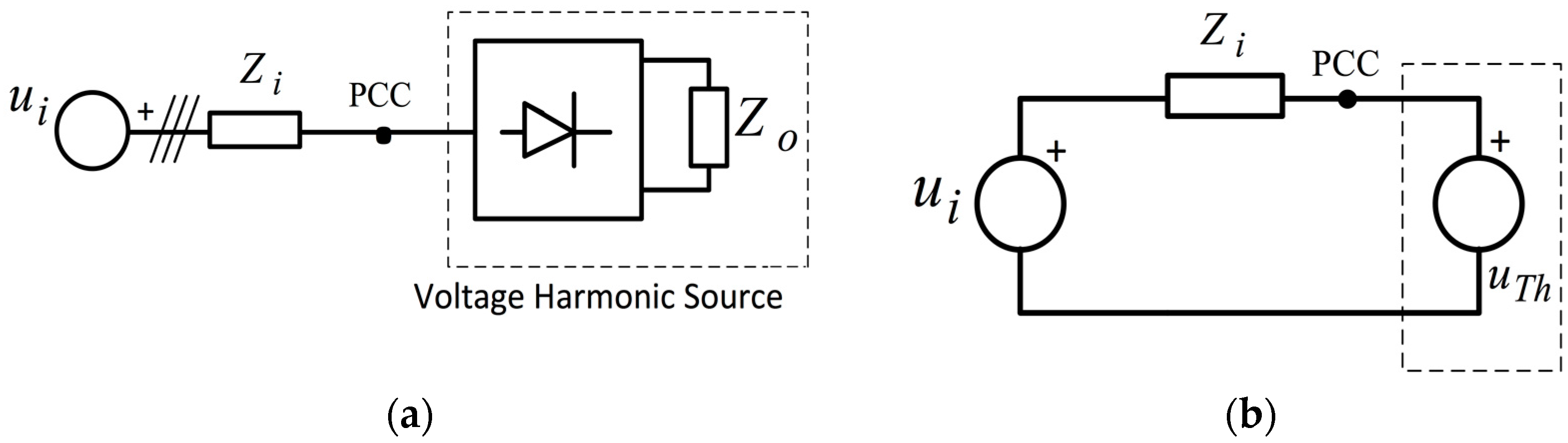
In order to show the validity of the energy conservation law stated in the above section, a numerical example is illustrated next. This theoretical applicaton case considers an example of a typical residential, commercial, and office load with harmonic voltage source behaviour, (see Section 3.2). As mentioned before, this kind of circuit is present in almost all residential, commercial, and industrial nonlinear loads, such as computers, video monitors, CCTV, electronic lamp ballasts, etc. The simplified equivalent circuit of these loads is assumed to be a diode rectifier with an output filter, as seen in Figure 6a,b.

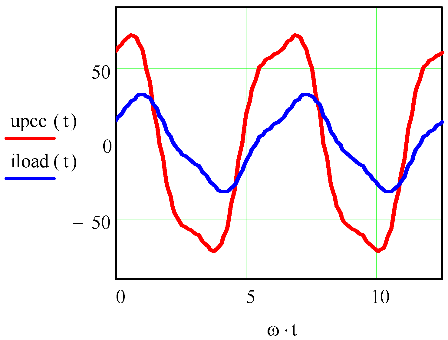
Figure 7 shows the instantaneous waveforms of the voltage and the load current, obtained by simulation at the PCC.

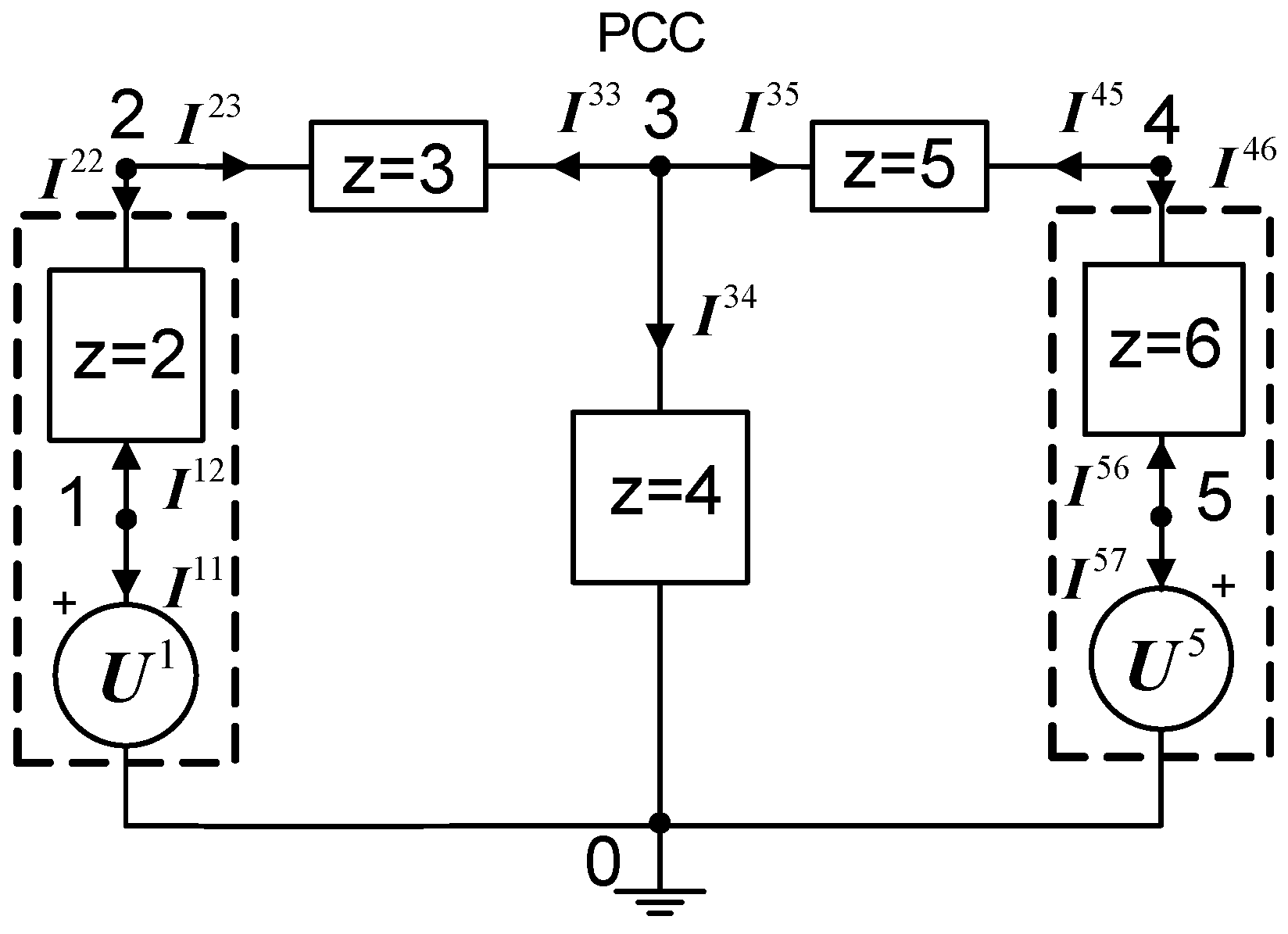
Conditioning the circuit of the Figure 6b, the equivalent circuit obtained, Figure 8, contains z (1,2…7)-elements and n = 1,2,...5 nodes.

In the proposed example, the instantaneous voltage sources at nodes 1 and 5 are given by

$$\begin{array}{ll}{u}^1(t)=220\sqrt{2}\sin (\omega t+\frac{\pi }{6})+5\sqrt{2}\sin (3\omega t+\frac{\pi }{3})& (V)\\ u^5(t)=100\sqrt{2}\sin (\omega t+\frac{\pi }{3})+25\sqrt{2}\sin (3\omega t-\frac{\pi }{6})& (V)\end{array}$$

In the new GCGA frequency domain framework their corresponding m-phasor $U^{\mathrm{n}}={\displaystyle \sum _{p\in \left\{1,3\right\}}{U}_{\mathrm{p}}^{\mathrm{n}}}$ are

$$\begin{array}{ll}{U}^1=U_1^1+U_3^1=220{\mathrm{e}}^{j30º}{\mathsf{\sigma }}_1+5{\mathrm{e}}^{j60º}{\mathsf{\sigma }}_3& (V)\\ U^5=U_1^5+U_3^5=100{\mathrm{e}}^{j60º}{\mathsf{\sigma }}_1+25{\mathrm{e}}^{-j30º}{\mathsf{\sigma }}_3& (V)\end{array}\}$$

(11)

and the resulting current m-phasors $I^{\mathrm{nz}}={\displaystyle \sum _{q\in \left\{1,3\right\}}{I}_{\mathrm{q}}^{\mathrm{nz}}}$ are given by

$$\begin{array}{ll}{I}^{11}=I_1^{11}+I_3^{11}=100.04{\mathrm{e}}^{-j133.90º}{\mathsf{\sigma }}_1+1.19{\mathrm{e}}^{-j30.96º}{\mathsf{\sigma }}_3=-I^{12}=I^{22}=-I^{23}=I^{33}& (A)\\ I^{34}=I_1^{34}+I_3^{34}=119.68{\mathrm{e}}^{j43.40º}{\mathsf{\sigma }}_1+2.25{\mathrm{e}}^{-j40.73º}{\mathsf{\sigma }}_3& (A)\\ I^{35}=I_1^{35}+I_3^{35}=20.31{\mathrm{e}}^{-j150.03º}{\mathsf{\sigma }}_1+3.43{\mathrm{e}}^{-j37.36º}{\mathsf{\sigma }}_3=I^{46}=I^{57}=-I^{45}=-I^{56}& (A)\end{array}\}$$

(12)

For each n-th node, and q-th harmonic, the equation of first Kirchhoff´s law can be rewritten in the following form:

$${\displaystyle \sum _{z=1}^Z{I}_{\mathrm{q}}^{\mathrm{nz}*}}=0$$

(13)

Multiplying (13) by the p-th voltage harmonic m-phasor in n-th node, $U_{\mathrm{p}}^{\mathrm{n}}$, the resulting equation still satisfies the null value,

$${\displaystyle \sum _{z=1}^Z{U}_{\mathrm{p}}^{\mathrm{n}}{I}_{\mathrm{q}}^{\mathrm{nz}*}}=0$$

(14)

where the sum is applied to all z-components connecting the n-th node.

The set (14) remains unaltered when all n-th nodes are considered,

$${\displaystyle \sum _{n=1}^N{\displaystyle \sum _{z=1}^Z{U}_{\mathrm{p}}^{\mathrm{n}}{I}_{\mathrm{q}}^{\mathrm{nz}*}}}=0$$

(15)

Equation (15) is the proposed generic expression of the power conservation law.

Applying (15), all the harmonic voltage sources and node-element harmonic currents are considered,

$$U_{\mathrm{p}}^1\left(I_{\mathrm{q}}^{11*}+I_{\mathrm{q}}^{12*}\right)+U_{\mathrm{p}}^2\left(I_{\mathrm{q}}^{22*}+I_{\mathrm{q}}^{23*}\right)+U_{\mathrm{p}}^3\left(I_{\mathrm{q}}^{33*}+I_{\mathrm{q}}^{34*}+I_{\mathrm{q}}^{35*}\right)+U_{\mathrm{p}}^4\left(I_{\mathrm{q}}^{45*}+I_{\mathrm{q}}^{46*}\right)+U_{\mathrm{p}}^5\left(I_{\mathrm{q}}^{56*}+I_{\mathrm{q}}^{57*}\right)=0$$

(16)

and grouping each associated z-element multivector-power,

$$\begin{array}{l}\underset{S_{\mathrm{pq}}^1}{\underbrace{U_{\mathrm{p}}^1{I}_{\mathrm{q}}^{11*}}}+\underset{S_{\mathrm{pq}}^2}{\underbrace{U_{\mathrm{p}}^1{I}_{\mathrm{q}}^{12*}+U_{\mathrm{p}}^2{I}_{\mathrm{q}}^{22*}}}+\underset{S_{\mathrm{pq}}^3}{\underbrace{U_{\mathrm{p}}^2{I}_{\mathrm{q}}^{23*}+U_{\mathrm{p}}^3{I}_{\mathrm{q}}^{33*}}}+\\ +\underset{S_{\mathrm{pq}}^4}{\underbrace{U_{\mathrm{p}}^3{I}_{\mathrm{q}}^{34*}}}+\underset{S_{\mathrm{pq}}^5}{\underbrace{U_{\mathrm{p}}^3{I}_{\mathrm{q}}^{35*}+U_{\mathrm{p}}^4{I}_{\mathrm{q}}^{45*}}}+\underset{S_{\mathrm{pq}}^6}{\underbrace{U_{\mathrm{p}}^4{I}_{\mathrm{q}}^{46*}+U_{\mathrm{p}}^5{I}_{\mathrm{q}}^{56*}}}+\underset{S_{\mathrm{pq}}^7}{\underbrace{U_{\mathrm{p}}^5{I}_{\mathrm{q}}^{57*}}}=0\end{array}$$

(17)

In general form

$$S_{\mathrm{pq}}={\displaystyle \sum _{z=1}^7{S}_{\mathrm{pq}}^{\mathrm{z}}=}{\displaystyle \sum _{z=1}^7{\displaystyle \sum _{n=1}^5{U}_{\mathrm{p}}^{\mathrm{n}}{I}_{\mathrm{q}}^{\mathrm{nz}*}}}=0$$

(18)

where the pq-th power component in a z-element is given by

$$S_{\mathrm{pq}}^{\mathrm{z}}=\underset{S_{\mathrm{pq}-\mathrm{Scalar}}}{\underbrace{\left({\mathrm{S}}_{11}^z+{\mathrm{S}}_{33}^z\right)}}{\mathsf{\sigma }}_0+\underset{S_{\mathrm{pq}-\mathrm{Bivector}}}{\underbrace{{\mathrm{S}}_{31}^z{\mathsf{\sigma }}_{31}}}=\underset{S_{\mathrm{pq}-\mathrm{Scalar}}}{\underbrace{\left({\mathrm{P}}^z+{\mathrm{jQ}}^z\right){\mathsf{\sigma }}_0}}+\underset{S_{\mathrm{pq}-\mathrm{Bivector}}}{\underbrace{{\mathrm{D}}_{31}^z{\mathsf{\sigma }}_{31}}}$$

(19)

From (17) and (19),

$$\begin{array}{l}Sources\{\begin{array}{l}{S}_{\mathrm{pq}}^{z=1}=\left(-21,145.66+6,110.64\mathrm{j}\right){\mathsf{\sigma }}_0+(473.69-131.94\mathrm{j}){\mathsf{\sigma }}_{31}\\ S_{\mathrm{pq}}^{z=7}=\left(-1,843.38-1,027.27\mathrm{j}\right){\mathsf{\sigma }}_0+(-210.16+99.56\mathrm{j}){\mathsf{\sigma }}_{31}\end{array}\\ \\ Loads\{\begin{array}{l}{S}_{\mathrm{pq}}^{z=2}=\left(10,009.72+30,0037.64\mathrm{j}\right){\mathsf{\sigma }}_0+(-1,448.01-509.07\mathrm{j}){\mathsf{\sigma }}_{31}\\ S_{\mathrm{pq}}^{z=3}=\left(10,009.72+60,052.70\mathrm{j}\right){\mathsf{\sigma }}_0+(-636.10+919.13\mathrm{j}){\mathsf{\sigma }}_{31}\\ S_{\mathrm{pq}}^{z=4}=28,679.2\mathrm{j}{\mathsf{\sigma }}_0+(1,072.39-110.25\mathrm{j}){\mathsf{\sigma }}_{31}\\ S_{\mathrm{pq}}^{z=5}=\left(848.46-3,747.53\mathrm{j}\right){\mathsf{\sigma }}_0+(395.16+15.62\mathrm{j}){\mathsf{\sigma }}_{31}\\ S_{\mathrm{pq}}^{z=6}=2,121.14{\mathsf{\sigma }}_0+(353.02-283.06\mathrm{j}){\mathsf{\sigma }}_{31}\end{array}\end{array}$$

(20)

According to (18), the global multivector apparent power is,

$$S={\displaystyle \sum _{p,q\in \left\{1,3\right\}}{S}_{\mathrm{pq}}=0}$$

(21)

From (19) and (21), when p = q it is possible to summarize the results expressed in (20) for those terms involving like frequency as $S_{Scalar-Sources}$ and $S_{Scalar-Loads}$. In this way,

$$\begin{array}{l}{S}_{Scalar-Sources}=\left(-29,989.05+5,083.37\mathrm{j}\right){\mathsf{\sigma }}_0(VA)\\ S_{Scalar-Loads}=\left(29,989.05-5,083.37\mathrm{j}\right){\mathsf{\sigma }}_0(VA)\end{array}\}\to S_{Scalar-Sources}+S_{Scalar-Loads}=0$$

(22)

where

$$\begin{array}{ll}{P}_{Sources}=P_{Loads}=29,989.05& (W)\\ Q_{Sources}=Q_{Loads}=5,083.37& (vad)\end{array}$$

(23)

where $\mathrm{P}$ and $\mathrm{Q}$ are the active and reactive powers defined in (6).

Similarly, when p ≠ q in (20), the summation of all cross-frequency terms are defined as $S_{Bivector-Sources}$ and $S_{Bivector-Loads}$:

$$\begin{array}{l}{S}_{Bivector-Sources}=D_{31-Sources}=\left(263.53-32.38\mathrm{j}\right){\mathsf{\sigma }}_{31}(vad)\\ S_{Bivector-Sources}=D_{31-Loads}=\left(-263.53+32.38\mathrm{j}\right){\mathsf{\sigma }}_{31}(vad)\end{array}\}\to D_{31-Sources}+D_{31-Loads}=0$$

(24)

where

$${\left|D_{31}\right|}_{Sources}={\left|D_{31}\right|}_{Loads}=265.51(vad)$$

(25)

and $D_{31}$ is the distortion bivector power defined in (6).

The proposed GCGA framework permits an easy geometric interpretation of the law of conservation of energy. It is possible to associate an Argand plane to each one of the considered basis or geometric objects: ${\mathsf{\sigma }}_0$ -plane or scalar complex plane and ${\mathsf{\sigma }}_{31}$ -plane or bivector complex plane (Figure 9). By this procedure, the quantities conservation problem reduces easily to real or imaginary components cancellation.

Note that the number of harmonics that can be considered depends only on computation constraints, because theoretically there are no limits due to the infinite dimension of the GCGA. The complex plane association extends to any geometric object, giving as a result a global conservation law by increasing the number of bivector planes.

It is remarkable that the proposed theory generalizes the Tellegen’s theorem for LTI (linear time-invariant) electric network operating in the AC steady state (often referred to in the European literature as Boucherot’s Theorem), to non-sinusoidal conditions. This is possible because of the natural additivity of the distortion bivector power in the GCGA framework. Thus, it can be stated that in non-sinusoidal, linear/nonlinear situations, not only both the sum of the active powers and the sum of reactive powers flowing into the branches are zero, but also the sum is null of distortion powers.

6. Conclusions

In this research, a new definition, interpretation and representation of electrical quantities such as voltage, current, and power terms are proposed based on GA framework. For this purpose a generalization of the classic Clifford algebra, which we have named “Generalized Complex Geometric Algebra” (GCGA), has been constructed. In this new framework a unified reformulation of power theory is provided. The proposed GCGA is consistent with Kirchhoff’s circuit laws, the principle of superposition and energy additivity, while Complex algebra circuit analysis framework is not. Particularly, this paper is aimed at yielding the following contributions:

• The traditional apparent power concept for industrial loads is unreliable: only in certain situations does it agree with the principle of conservation of energy, and as a result, it can lead to erroneous conclusion. This power concept must be revisited. The classical tools based simply on complex numbers are not enough to achieve this goal.
• In contrast to the classical concept of the apparent power, the proposed definition as a power multivector considers the net flow of all the power components present in industrial electric loads.
• The distinct nature of power components is easily differentiated in this algebra. This permits obtainment of a general proof of the principle of conservation energy for linear and nonlinear loads in non-sinusoidal conditions: the volt-amperes at the input terminal equals the sum of the volt-amperes at each load component.
• The proposed GCGA framework permits an easy geometric interpretation of the law of conservation of energy based on complex geometric objects.
• The distortion power achieves the additivity property.
• The multivector power theory generalizes the Tellegen´s theorem for LTI power systems operating in the AC non-sinusoidal steady state.

References

1. Wagner, V.E.; Balda, J.C.; Barnes, T.M.; Emannuel, A.E.; Ferraro, R.J.; Griffith, D.C.; Hartmann, D.P.; Horton, W.F.; Jewell, W.T.; McEachern, A.; et al. Effects of harmonics on equipment. IEEE Trans. Power Delivery 1993, 8, 672–680. [Google Scholar] [CrossRef]
2. Henderson, R.D.; Rose, P.J. Harmonics: The effects on power quality and transformers. IEEE Trans. Ind. Applicat. 1994, 30, 528–532. [Google Scholar] [CrossRef]
3. Budeanu, C.I. Puisances Reactives et Fictives; Instytut Romain de l´Energie: Bucharest, Romania, 1927. [Google Scholar]
4. Shepherd, W.; Zhakikhani, P. Suggested definition of reactive power for nonsinusoidal systems. Proc. Inst. Elect. Eng. 1972, 119, 1361–1362. [Google Scholar] [CrossRef]
5. Czarnecki, L.S. Considerations on the reactive power in non-sinusoidal situations. IEEE Trans. Instr. Meas. 1985, 34, 399–404. [Google Scholar] [CrossRef]
6. Sharon, D. Reactive power definitions and power factor improvement in nonlinear systems. Proc. IEE 1973, 120, 6. [Google Scholar] [CrossRef]
7. Ghassemi, F. New Apparent Power and Power Factor with Non-Sinusoidal waveforms. Power Eng. Soc. Winter Meet. 2000, 4, 2852–2857. [Google Scholar]
8. Slonim, M.A.; Van Wyk, J.D. Powers components in a system with sinusoidal and nonsinusoidal voltages and/or currents. Proc. Inst. Elect Eng. 1988, 135, 76–84. [Google Scholar] [CrossRef]
9. LaWhite, N.; Ilic, M.D. Vector Space Decomposition of Reactive Power for Periodic Nonsinusoidal Signals. IEEE Trans. Circuits Syst. 1997, 44, 4. [Google Scholar] [CrossRef]
10. Sommariva, A.M. Power Analysis of One-Ports Under Periodic Multi-Sinusoidal Operation. IEEE Trans. Circuits Syst. 2006, 53, 9. [Google Scholar] [CrossRef]
11. Castilla, M.; Bravo, J.C.; Ordoñez, M.; Montaño, J.C. Clifford Theory: A geometrical interpretation of multivectorial apparent power. IEEE Trans. Circuits Syst. 2008, 55, 10. [Google Scholar] [CrossRef]
12. Shepherd, W.; Zand, P. Energy Flow and Power Factor in Nonsinusoidal Circuits; Cambridge University Press: London, UK, 1979. [Google Scholar]
13. Castilla, M.; Bravo, J.C.; Ordoñez, M.; Montaño, J.C. An Approach to the multivectorial apparent power in terms of a generalized poynting multivector. Prog. Electromagnet. Res. 2009, 15, 401–422. [Google Scholar] [CrossRef]
14. Castilla, M.; Bravo, J.C.; Ordoñez, M.; Montaño, J.C. The geometric algebra as a power theory analysis Tool. Przeglad Elektrochniczny 2009, 1, 202–207. [Google Scholar]
15. Menti, A.; Zacharias, T.; Milias-Argitis, J. Geometric Algebra: A powerful tool for representing power under nonsinusoidal conditions. IEEE Trans. Circuits Syst. 2007, 54, 601–609. [Google Scholar] [CrossRef]
16. Castro-Núñez, M.; Castro-Puche, R. Advantages of geometric algebra over complex numbers in the analysis of Networks with nonsinusoidal Sources and Linear Loads. IEEE Trans. Circuits Syst. 2012, 59, 2056–2064. [Google Scholar] [CrossRef]
17. Clifford, W.K. On the classification of Geometric Algebras. In Mathematical Papers; Tucker, R., Ed.; Macmilliam: London, UK, 1882; pp. 397–405. [Google Scholar]
18. Doran, C.; Lasenby, A. Geometric Algebra for Physicists; Cambridge University Press: London, UK, 2003. [Google Scholar]
19. Ventkastesh, C.; Srikanth, D.; Siva Sarma, D.V.S.S.; Sidulu, M. Modelling of nonlinear loads and estimation of harmonic in industrial distribution system. In Proceedings of the Fifteenth National Power Systems Conference, Bombay, India, 16–18 December 2008.
20. Pomilio, J.A.; Deckmann, S.M. Characterization and compensation of harmonics and reactive Power of residential and commercial loads. IEEE Trans. Power Delivery 2007, 2, 2. [Google Scholar] [CrossRef]
21. Castilla, M.; Bravo, J.C.; Ordoñez, M. Geometric algebra: A multivectorial proof of Tellegen’s theorem in multiterminal networks. IET Circuits, Devices Syst. 2008, 2, 4. [Google Scholar] [CrossRef]
Figure 1. Basis sets of G3: scalar as point, vectors as directed line segments, bivectors as oriented planes, and trivector as oriented volume.
Symmetry 08 00092 g001
Figure 2. (a) Simplified three-phase thyristor rectifier. (b) Equivalent circuit.
Symmetry 08 00092 g002
Figure 3. (a) Simplified three phase diode rectifier and (b) Equivalent circuit.
Symmetry 08 00092 g003
Figure 4. Phase of a generic industrial building load.
Symmetry 08 00092 g004
Figure 5. z-element signs criteria.
Symmetry 08 00092 g005
Figure 6. (a,b) Load fed by rectifier and harmonic voltage source equivalent, both with shunt filter.
Symmetry 08 00092 g006
Figure 7. PCC distorted voltage and load current.
Symmetry 08 00092 g007
Figure 8. Conditioned equivalent circuit.
Symmetry 08 00092 g008
Figure 9. (a) σ 0 -plane: active and reactive power conservation; (b) σ 31 -plane: distortion power conservation.
Symmetry 08 00092 g009