A Recourse-Based Type-2 Fuzzy Programming Method for Water Pollution Control under Uncertainty

Abstract

In this study, a recourse-based type-2 fuzzy programming (RTFP) method is developed for supporting water pollution control of basin systems under uncertainty. The RTFP method incorporates type-2 fuzzy programming (TFP) within a two-stage stochastic programming with recourse (TSP) framework to handle uncertainties expressed as type-2 fuzzy sets (i.e., a fuzzy set in which the membership function is also fuzzy) and probability distributions, as well as to reflect the trade-offs between conflicting economic benefits and penalties due to violated policies. The RTFP method is then applied to a real case of water pollution control in the Heshui River Basin (a rural area of China), where chemical oxygen demand (COD), total nitrogen (TN), total phosphorus (TP), and soil loss are selected as major indicators to identify the water pollution control strategies. Solutions of optimal production plans of economic activities under each probabilistic pollutant discharge allowance level and membership grades are obtained. The results are helpful for the authorities in exploring the trade-off between economic objective and pollutant discharge decision-making based on river water pollution control.

1. Introduction

The trade-off between water pollution control and economic development is of great concern in many basins since it is essential to local sustainable development [1,2]. It is difficult to keep the economy growing under the utilization of water resources and the deterioration of environmental conditions [3,4]. Meanwhile, it is hard to promote human society improvement if the authorities excessively restrict economic development. Under such a contradictory situation, optimization techniques are proper to detect the economic and environmental impacts of alternative pollution control actions from a system point of view, and thus aid the authorities in formulating and adopting cost-effective water pollution plans and policies. However, water pollution control planning is governed by significant sources of uncertainty associated with different variables, and uncertainty is a non-negligible constituent of such a procedure [5]. There are significant uncertainties in not only how the system might develop, but also in how the system is expected to adjust when many system components are altered (e.g., pollutant discharge amount, cost/benefit coefficient and economic activity scale).

In water pollution control problems, values of associated parameters (e.g., cost/benefit coefficients) are usually determined via tests, experiences and expertises, while these methods may fail in determining accurate values, resulting in the parameters being described by fuzzy membership functions. Such deviations in subjective estimations can lead to fuzziness being inherent in the real-world decision problems (e.g., vagueness and/or impreciseness in the outcomes of a water pollution control sample), neglect of which can cause the solutions of problems deviating greatly from their true values. Fuzzy mathematic programming (FMP), based on fuzzy sets theory, can facilitate the analysis of system associated with uncertainties being derived from vagueness and imprecision [6,7]. FMP is capable of handling decision problems under fuzzy goal and constraints and tackling ambiguous coefficients in the objective function and constraints. Previously, a wide range of FMP methods were developed for water pollution control [8,9,10,11,12,13,14,15]. For example, Liu et al. [16] improved a two-stage fuzzy robust programming model for water pollution control to address fuzzy parameters, which were represented by possibility distributions on the left- and right-hand sides of the constraints. Tavakoli et al. [17] developed an interactive two-stage stochastic fuzzy programming method to handle uncertainties expressed as fuzzy boundary intervals (i.e., the lower- and upper-bounds of intervals are presented as possibility distributions). Ji et al. [18] enhanced an inexact left-hand-side chance-constrained fuzzy multi-objective programming approach to cope with fuzziness in the constraints and objectives. Generally, the conventional fuzzy programming methods could only tackle fuzzy uncertainty with precise membership grades, which may encounter difficulty when the membership grades are also obtained as fuzzy sets.

In many real-world situations, related data such as unit net benefits of economic activities and pollutant discharge allowances are often highly uncertain, which could not be handled by the conventional fuzzy programming methods. When it is challenging to identify the membership grade of a fuzzy set as crisp values (e.g., unit benefit), type-2 fuzzy sets (T2FS) can effectively determine the membership function through defying membership grades of T2FS are fuzzy sets within [0,1] [19,20,21,22]. In addition, membership functions cannot express uncertainties featured with randomness. Two-stage stochastic programming with recourse is effective for handling decision-making problems in which an examination of policy levels is desired and the system data is characterized by uncertainty [23]. Therefore, as an extension to the existing approaches, a recourse-based type-2 fuzzy programming (RTFP) method incorporating the concepts of type-2 fuzzy programming (TFP) within a two-stage stochastic programming with recourse (TSP) framework will be developed to address the above deficiencies. Then, the RTFP method will be applied to water pollution control in the Heshui River Basin in China. Results of optimal agriculture, industry, forestry, fishery, and livestock husbandry activities will be generated, which will be used for providing insight into the trade-off among system benefit, water pollution control, and sustainability.

2. Methodology

In water pollution control decision making problems, uncertainties may arise due to subjective estimation. For instance, decision makers may estimate the unit benefit from planting fruit/vegetable being [424.1, 575.6] × 10³ $/km² with additional information as the possibility of “the most possible unit benefit of 499.8 × 10³ $/km²” is 0.8, and the possibilities of ‘‘there is no possibility that the unit benefit is lower than 424.1 × 10³ $/km² or higher than 575.6 × 10³ $/km²” are 0.2 and 0.3, respectively. Under such a situation, unit benefit from planting fruit/vegetable should be described as type-2 fuzzy sets (T2FS). Thus, type-2 fuzzy programming (TFP) can be adopted to tackle such uncertainties, which can be presented as [24]:

$$\mathrm{Max}f=\tilde{C}X,$$

(1)

subject to:

$$\tilde{A}X\le B,$$

(2)

$$X\ge 0,$$

(3)

where $\tilde{C}\in {\left\{R\right\}}^{1\times n}$ and $\tilde{A}\in {\left\{R\right\}}^{m\times n}$ are vectors of T2FS. A type-2 fuzzy set $\tilde{C}$ in $X$ is a fuzzy set in which the membership function is also fuzzy (i.e., type-2 membership function). The $\tilde{C}$ defined on the universe of discourse $X$ is represented as [25]:

$$\tilde{C}=\{((x,u),{\mu }_{\tilde{C}}(x,u)):\forall x\in X,\forall u\in J_x\subseteq [0,1]\},$$

(4)

where $0\le {\mu }_{\tilde{C}}(x,u)\le 1$ is the type-2 membership function, $J_x\subseteq [0,1]$ is the primary membership of $x\in X$, which is the domain of the secondary membership function ${\mu }_{\tilde{C}}(x)$ so that all $u\in J_x$ are the primary membership grades of the point x. The secondary membership function of a triangular $\tilde{C}=(c_1,c_2,c_3,{\theta }_1,{\theta }_r)$ can be defined as:

$${\mu }_{\tilde{C}}(x)=\{\begin{array}{l}(\frac{x-c_1}{c_2-c_1}-{\theta }_1\frac{x-c_1}{c_2-c_1},\frac{x-c_1}{c_2-c_1},\frac{x-c_1}{c_2-c_1}+{\theta }_r\frac{x-c_1}{c_2-c_1}),\mathrm{if}x\in [c_1,\frac{c_1+c_2}{2}]\\ (\frac{x-c_1}{c_2-c_1}-{\theta }_1\frac{c_2-x}{c_2-c_1},\frac{x-c_1}{c_2-c_1},\frac{x-c_1}{c_2-c_1}+{\theta }_r\frac{c_2-x}{c_2-c_1}),\mathrm{if}x\in [\frac{c_1+c_2}{2},c_2]\\ (\frac{c_3-x}{c_3-c_2}-{\theta }_1\frac{x-c_2}{c_3-c_2},\frac{c_3-x}{c_3-c_2},\frac{c_3-x}{c_3-c_2}+{\theta }_r\frac{x-c_2}{c_3-c_2}),\mathrm{if}x\in [c_1,\frac{c_2+c_3}{2}]\\ (\frac{c_3-x}{c_3-c_2}-{\theta }_1\frac{c_3-x}{c_3-c_2},\frac{c_3-x}{c_3-c_2},\frac{c_3-x}{c_3-c_2}+{\theta }_r\frac{c_3-x}{c_3-c_2}),\mathrm{if}x\in [\frac{c_2+c_3}{2},c_2]\end{array},$$

(5)

where $c_1$, $c_2$, $c_3$ are real numbers and ${\theta }_1$; ${\theta }_r\in [0,1]$ are two parameters representing the spreads of primary membership grades of $\tilde{C}$.

One of the main limitations of the TFP method remains in its difficulty in coping with uncertainties described as probability distributions when the available historical data is sufficient (e.g., pollutant discharge allowances) [26,27,28]. Such a problem can be formulated as a two-stage stochastic programming with a recourse (TSP) model [23]. Through incorporating the TFP method within the TSP framework, a recourse-based type-2 fuzzy programming (RTFP) method can be formulated as follows:

$$\mathrm{Max}f={\displaystyle \sum _{j=1}^{n_1}{\tilde{c}}_j{x}_j}-{\displaystyle \sum _{j=1}^{n_2}{\displaystyle \sum _{s=1}^S{p}_s{\tilde{e}}_j{y}_{js}}},$$

(6)

subject to:

$${\displaystyle \sum _{j=1}^{n_1}{\tilde{a}}_{rj}{x}_j}\le {\tilde{b}}_r,r=1,2,\dots ,m_1,$$

(7)

$${\displaystyle \sum _{j=1}^{n_1}{a}_{tj}{x}_j}+{\displaystyle \sum _{j=1}^{n_2}{a}_{tj}^{\prime }{y}_{jts}}\le {\omega }_s,t=1,2,\dots ,m_2;s=1,2,\dots ,v,$$

(8)

$$x_j\ge 0,j=1,2,\dots ,n_2,$$

(9)

$${\mathrm{y}}_{js}\ge 0,j=1,2,\dots ,n_2;s=1,2,\dots ,v.$$

(10)

Decision variables are divided into two subsets: those that must be determined before the realizations of random variables are known, and those (recourse variables) that are determined after the realized random variables are disclosed. $x_j$ is the first-stage decision made before the random variable is observed, ${\omega }_s$ is the random variable with a probability level $p_s$ (i.e., the probability of realization of ${\omega }_s$, with $p_s>0$ and ${\displaystyle {\sum }_{s=1}^S{p}_s}=1$) [29], and $y_{js}$ is the second-stage adaptive decision, which depends on the realization of the random variable. ${\displaystyle \sum _{j=1}^{n_2}{\tilde{e}}_j{y}_{js}}$ denotes the second-stage cost function (${\tilde{e}}_j$ is cost coefficient of $y_{js}$). Inequality (4e) presents the relationship among $x_j$, $y_{js}$, and ${\omega }_s$.

An extra type reduction is needed to convert the output of T2FS into conventional fuzzy sets so that they can be defuzzified to give crisp outputs. Suppose that $h_1$, $h_2$, …, $h_i$ are the value of ${\tilde{c}}_{ij}$ (for at least one pair of $i\ne j$, define $h_i\ne h_j$) evaluated by $t$ different experts. The relative distances of $h_i$ are used to approximate the center. Values lying closer to the center are considered more important. Generally, the fuzzification of ${\tilde{c}}_{ij}$ can be represented as: (1) calculate the relative distance matrix $D=|d_{ij}{|}_{t\times t}$, where $d_{ij}=|h_i-h_j|$; (2) calculate the average of relative distances ${\overline{d}}_i={\displaystyle {\sum }_{i=1}^t{d}_{ij}/(t-1)}$; (3) introduce a pair-wise comparison $p_{ij}$ ($p_{ij}={\overline{d}}_j/{\overline{d}}_i$), and the pair-wise matrix $P=|p_{ij}{|}_{t\times t}$; (4) obtain the true-importance degree $w_i$ of $h_i$ ($w_j=1/{\displaystyle {\sum }_{j=1}^t{p}_{ij}}$); (5) assess the mode of m ($m={\displaystyle {\sum }_{i=1}^t{w}_i{h}_i}$) of the fuzzy number; (6) choose $s={\displaystyle {\sum }_{i=1}^t{w}_i|h_i-m|}$ to approximate the unknown mean deviation σ; (7) acquire the ratio of left spread to the right spread $\eta =(m-h^l)/(h^{\prime }-m)$, with $h^l={\displaystyle {\sum }_{i\in A}{w}_i{h}_i}/{\displaystyle {\sum }_{i\in A}{w}_i}$, $h^{\prime }={\displaystyle {\sum }_{i\in B}{w}_i{h}_i}/{\displaystyle {\sum }_{i\in B}{w}_i}$, $A=\left\{i\right|h_i<m,i\in I\}$, $B=\left\{i\right|h_i>m,i\in I\}$ and $I=\{1,2,\dots ,t\}$; (8) obtain $a=m-3(1+\eta )\eta \sigma /(1+{\eta }^2)$ and $b=m+3(1+\eta )\sigma /(1+{\eta }^2)$. The conventional fuzzy number $F=(a,m,b)$ of ${\tilde{c}}_{ij}$ can thus be acquired. Then, the defuzzification of T2FS can be conducted according to the critical value (CV)-based reduction method [30].

Suppose that $\tilde{c}$ is a triangular type-2 fuzzy variable with secondary possibility distribution function ${\mu }_{\tilde{c}}(x)$ (which represents a regular fuzzy variable). The method is introducing the CVs as representing values of the regular fuzzy variable ${\mu }_{\tilde{c}}(x)$, i.e., $C{V}^{*}[{\mu }_{\tilde{c}}(x)]$ (optimistic CV), $C{V}_{*}[{\mu }_{\tilde{c}}(x)]$ (pessimistic CV) and $CV[{\mu }_{\tilde{c}}(x)]$. Then, the corresponding fuzzy variables are derived using these CVs of the secondary possibilities:

$$\tilde{c}=\left(\begin{array}{ccc}{\alpha }_1& {\alpha }_2& {\alpha }_3\\ m& 1& n\end{array}\right),$$

(11)

where ${\alpha }_1$, ${\alpha }_2$, and ${\alpha }_3$ are primary membership grade of $\tilde{c}$, and m, 1, and n are corresponding secondary membership grades.

$$Pos(\tilde{c}\ge \alpha )=\underset{r\ge \alpha }{\sup }{\mu }_{\tilde{c}}(r)=\{\begin{array}{l}1\mathrm{if}0\le \alpha \le {\alpha }_2\\ n\mathrm{if}{\alpha }_2\le \alpha \le {\alpha }_3\\ 0\mathrm{if}{\alpha }_3\le \alpha \le 1\end{array},$$

(12)

$$Nec(\tilde{c}\ge \alpha )=1-\underset{r<\alpha }{\sup }{\mu }_{\tilde{c}}(r)=\{\begin{array}{l}1\mathrm{if}0\le \alpha \le {\alpha }_1\\ m\mathrm{if}{\alpha }_1\le \alpha \le {\alpha }_2\\ 0\mathrm{if}{\alpha }_2\le \alpha \le 1\end{array},$$

(13)

$$Cr\{\tilde{c}\ge \alpha \}=\frac{1}{2}(Pos(\tilde{c}\ge \alpha )+Nec(\tilde{c}\ge \alpha ))=\{\begin{array}{ll}1& \mathrm{if}0\le \alpha \le {\alpha }_1\\ \frac{1+m}{2}& \mathrm{if}{\alpha }_1\le \alpha \le {\alpha }_2\\ \frac{n}{2}& \mathrm{if}{\alpha }_2\le \alpha \le {\alpha }_3\\ 0& \mathrm{if}{\alpha }_3\le \alpha \le 1\end{array}.$$

(14)

Then, $C{V}^{*}[{\mu }_{\tilde{c}}(x)]$, $C{V}_{*}[{\mu }_{\tilde{c}}(x)]$ and $CV[{\mu }_{\tilde{c}}(x)]$ are defined as follows:

$$C{V}^{*}(\tilde{c})=\underset{\alpha \in [0,1]}{\sup }(\alpha \wedge Pos\{\tilde{c}\ge \alpha \}),$$

(15)

$$C{V}_{*}(\tilde{c})=\underset{\alpha \in [0,1]}{\sup }(\alpha \wedge Nes\{\tilde{c}\ge \alpha \}),$$

(16)

$$CV(\tilde{c})=\underset{\alpha \in [0,1]}{\sup }(\alpha \wedge Cr\{\tilde{c}\ge \alpha \}).$$

(17)

Finally, to obtain crisp values, centroid method (${\displaystyle {\sum }_{x}x{\mu }_{\tilde{c}}(x)}/{\displaystyle {\sum }_x{\mu }_{\tilde{c}}(x)}$) is used for these reduced conventional fuzzy variables. Generally, the detailed computational processes for solving the RTFP method can be summarized as follows:

Step 1.

Formulate the RTFP model.

Step 2.

Discrete probability distribution into several values with each corresponds to one probability.

Step 3.

Convert the output of T2FS into conventional fuzzy sets.

Step 4.

Conduct defuzzification of T2FS according to the critical value (CV)-based reduction method.

Step 5.

Run the RTFP model.

Step 6.

Obtain the optimal solutions of the objective function ($f$), first-stage decision variable ($x_j$), and second-stage decision variable ($y_{js}$).

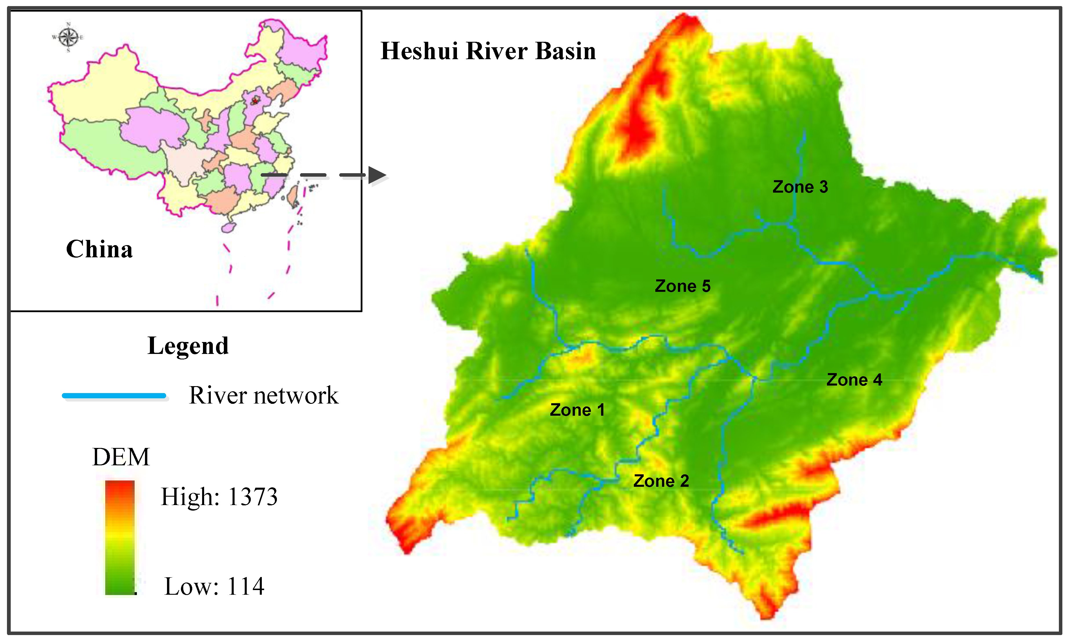
3. Case Study

Yongxin, a county of Jiangxi Province, is located in the southeast part of China (as shown in Figure 1). It ranges in longitude from 113.83° E to 114.31° E, and in latitude from 26.78° N to 27.23° N. It occupies a total area of around 2194.57 km², and the majority of the county (i.e., approximately 1800 km²) lies within the middle reaches of the Heshui River Basin [31]. The basin features subtropical monsoon humid climatic conditions (abundant rainfall and sunlight, and long frost-free periods) with an average annual precipitation of 1530.7 mm and an average annual temperature of 18.2 °C. The Heshui River has a total length of 225 km, with 77 km flowing within the borders of Yongxin County from west to east. The county mainly relies on the Heshui River to support its agriculture, industry, livestock husbandry, forestry, and fishery [32].

In the county, farmland, orchard, and woodland occupy15.2%, 0.6%, and 70.1% of the total land, receptively. Grassland accounts for 6.1% of the total area, most of which is in good condition and suitable for feeding a large number of livestock. Land for urban construction, traffic, and water conservancy facilities cover 3.4%, 0.4%, and 0.6% of the total land, respectively. Agriculture is traditionally the primary sector of the County. Paddy soil is the main cultivation soil type, and it is not only suitable for rice planting but can also be used for rapeseeds and other cash crops. Fruit orchards produce a variety of fruits such as pear, peach, orange and plum. Agriculture includes paddy, dry and vegetable/fruit farms. The main types of livestock raised in the County are hogs, cattle and poultry. Pork and beef account for around 75.5 and 13.2% of the total meat production, respectively. The second industrial sector in the county is mainly comprised of mining, manufacturing, construction, transportation and other industries. The area possesses more than 20 types of mineral deposits, and the mineral production was 315.0 thousand tonnes [32,33].

In the past twenty years, driven by poverty, authorities have given top priority to the booming economy in the local strategic plans [33]. According to the report of local government in 2016, the total population was approximately 53,139, and the net income per capita was 8520 Chinese yuan (approximately $1290). One major environmental issue in the study area is water pollution, which is mainly caused by excessive pollutant loadings from agriculture, forestry, fishery, and livestock husbandry, and industry. Water pollution problems pose great obstacles to sustainable development in the county; thus, it is essential to optimize economic structure from a systematic point of view. Based on field investigations and related literature, chemical oxygen demand (COD), total nitrogen (TN), total phosphorus (TP), and soil loss have been selected as the pollutant types to control water pollution. Five zones (zones 1 to 5) are chosen to control water pollution. After the first-stage decisions (i.e., planning targets of economic activities) are made, associated pollution, the amount of which is in proportion to the economic production, is discharged into the water body. Based on the calculation of discharged wastewater and the measurement of incoming water quality, the mitigation schemes can be determined as the second-stage decisions in order to meet the environmental standards. If the production targets of them are made too high, the additionally generated pollutants will have to be mitigated in a more expensive way or discharged/drained into the stream (leading to penalties from the government). Conversely, if the production targets are made too low, the system will encounter opportunity losses of economic income, leading to a reduced system benefit. The pollutant discharge allowances are highly uncertain, which are presented as probability distributions. Seven pollutant-discharge allowance levels are generated in association with different probabilities, which are identified as very-low, low, low-medium, medium, medium-high, high, and very-high, respectively. More uncertainties associated with cost/benefit coefficients may come from measurement errors and/or subjective judgment, and they can be expressed as T2FS. Therefore, the developed RTFP method can be adopted to plan water pollution control in the study area. The formulation of the RTFP model is presented as follows:

$$\begin{array}{cc}\hfill \mathrm{Max}{f}^{\pm }=& {\displaystyle \sum _{i=1}^{I_a}{\displaystyle \sum _{j=1}^J\tilde{B}{A}_{ij}^{}\cdot T{A}_{ij}^{}(+\mathrm{\Delta }T{A}_{ij}{u}_{ij})}}-{\displaystyle \sum _{i=1}^{I_a}{\displaystyle \sum _{j=1}^J{\displaystyle \sum _{h=1}^H{\displaystyle \sum _{k=2}^K{p}_h\cdot PE{A}_{ik}^{}\cdot \tilde{D}P{A}_{ijk}^{}\cdot X{A}_{ijhk}^{}}}}}\hfill \\ & +{\displaystyle \sum _{i=1}^{I_f}{\displaystyle \sum _{j=1}^J\tilde{B}{F}_{ij}^{}\cdot T{F}_{ij}^{}}}-{\displaystyle \sum _{i=1}^{I_f}{\displaystyle \sum _{j=1}^J{\displaystyle \sum _{h=1}^H{\displaystyle \sum _{k=1}^{K-1}{p}_h\cdot PE{F}_{ik}^{}\cdot \tilde{D}P{F}_{ijk}^{}\cdot X{F}_{ijhk}^{}}}}}\hfill \\ & +{\displaystyle \sum _{i=1}^{I_l}{\displaystyle \sum _{j=1}^J\tilde{B}{L}_{ij}^{}\cdot T{L}_{ij}^{}}}-{\displaystyle \sum _{i=1}^{I_l}{\displaystyle \sum _{j=1}^J{\displaystyle \sum _{h=1}^H{p}_h\cdot PE{L}_i^{}\cdot \tilde{D}P{L}_{ij}^{}\cdot X{L}_{ijh}^{}}}}\hfill \\ & {\displaystyle \sum _{i=1}^{I_i}{\displaystyle \sum _{j=1}^{J}T{I}_{ij}^{}}}-{\displaystyle \sum _{i=1}^{I_i}{\displaystyle \sum _{j=1}^J{\displaystyle \sum _{h=1}^H{p}_h\cdot PE{I}_i^{\pm }\cdot \tilde{D}P{I}_{ij}^{}\cdot X{I}_{ijh}^{}}}}\hfill \\ & +{\displaystyle \sum _{i=1}^{I_w}{\displaystyle \sum _{j=1}^J\tilde{B}{W}_{ij}^{}\cdot T{W}_{ij}^{}}}-{\displaystyle \sum _{i=1}^{I_i}{\displaystyle \sum _{j=1}^J{\displaystyle \sum _{h=1}^H{p}_h\cdot PE{W}_i^{}\cdot \tilde{D}P{W}_{ij}^{}\cdot X{W}_{ijh}^{}}}}\hfill \end{array}$$

(18)

(1)

COD discharge constraints:

$${\displaystyle \sum _{i=1}^{I_f}(T{F}_{ij}^{}-X{F}_{ijh}^{})\cdot CC{O}_{ij}^{}}\le PC{F}_{jh}^{},\forall j,h,$$

(19)

$${\displaystyle \sum _{i=1}^{I_i}(T{L}_{ij}^{}-X{L}_{ijh}^{})\cdot DP{L}_{ij}^{\pm }}\le PC{L}_{jh}^{},\forall j,h,$$

(20)

$${\displaystyle \sum _{i=1}^{I_i}(T{I}_{ij}^{}-X{I}_{ijh}^{})}\cdot DP{I}_{ij}^{\pm }\le PC{I}_{jh}^{},\forall j,h,$$

(21)

$$\begin{array}{l}{\displaystyle \sum _{j=1}^J[{\displaystyle \sum _{i=1}^{I_f}(T{F}_{ij}^{}-X{F}_{ijh}^{})\cdot CC{O}_{ij}^{}}+{\displaystyle \sum _{i=1}^{I_i}(T{L}_{ij}^{}-X{L}_{ijh}^{})\cdot DP{L}_{ij}^{}}}\\ +{\displaystyle \sum _{i=1}^{I_i}(T{I}_{ij}^{}-X{I}_{ijh}^{})}\cdot DP{I}_{ij}^{}]\le MC{L}_h^{},\forall h\end{array},$$

(22)

(2)

Phosphorus discharge constraints:

$${\displaystyle \sum _{i=1}^{I_a}(T{A}_{ij}^{}-X{A}_{ijh}^{})\cdot (S{L}_{ij}^{}\cdot A{P}_{ij}^{}+R{A}_{ij}^{}\cdot R{P}_{ij}^{})}\le PA{P}_{jh}^{},\forall j,h,$$

(23)

$${\displaystyle \sum _{i=1}^{I_f}(T{F}_{ij}^{}-X{F}_{ijh}^{})\cdot F{P}_{ij}^{\pm }}\le PF{P}_{jh}^{},\forall j,h,$$

(24)

$$\begin{array}{l}{\displaystyle \sum _{j=1}^J[{\displaystyle \sum _{i=1}^{I_a}(T{A}_{ij}^{}-X{A}_{ijh}^{})\cdot (S{L}_{ij}^{}\cdot A{P}_{ij}^{}+R{A}_{ij}^{}\cdot R{P}_{ij}^{})}}\\ +{\displaystyle \sum _{i=1}^{I_f}(T{F}_{ij}^{}-X{F}_{ijh}^{})\cdot F{P}_{ij}^{}}]\le MP{L}_h^{},\forall h\end{array},$$

(25)

(3)

Nitrogen discharge constraints:

$${\displaystyle \sum _{i=1}^{I_{}}(T{A}_{ij}^{}-X{A}_{ijh}^{})\cdot (S{L}_{ij}^{}\cdot A{N}_{ij}^{}+R{A}_{ij}^{}R{N}_{ij}^{})}\le PA{N}_{jh}^{},\forall j,h,$$

(26)

$${\displaystyle \sum _{i=1}^{I_f}(T{F}_{ij}^{}-X{F}_{ijh}^{})\cdot F{N}_{ij}^{}}\le PF{N}_{jh}^{},\forall j,h,$$

(27)

$$\begin{array}{l}{\displaystyle \sum _{i=1}^{I_a}(T{A}_{ij}^{}-X{A}_{ijh}^{})\cdot (S{L}_{ij}^{}\cdot A{N}_{ij}^{}+R{A}_{ij}^{}\cdot R{N}_{ij}^{})}\\ +{\displaystyle \sum _{i=1}^{I_f}(T{F}_{ij}^{}-X{F}_{ijh}^{})\cdot F{N}_{ij}^{}}\le MN{L}_h^{},\forall h\end{array},$$

(28)

(4)

Soil loss constraints:

$${\displaystyle \sum _{i=1}^{I_i}(T{A}_{ij}^{}-X{A}_{ijh}^{})\cdot S{L}_{ij}^{}}\le PS{L}_{jh}^{},\forall j,h,$$

(29)

$${\displaystyle \sum _{i=1}^{I_w}(T{W}_{ij}^{}-X{W}_{ijh}^{})\cdot DP{W}_{ij}^{}}\le PW{S}_{jh}^{},\forall j,h,$$

(30)

$$\begin{array}{l}{\displaystyle \sum _{j=1}^J[{\displaystyle \sum _{i=1}^{I_i}(T{A}_{ij}^{}-X{A}_{ijh}^{})\cdot S{L}_{ij}^{\pm }}}\\ +{\displaystyle \sum _{i=1}^{I_w}(T{W}_{ij}^{}-X{W}_{ijh}^{})\cdot DP{W}_{ij}^{}}]\le MS{L}_h^{},\forall h\end{array},$$

(31)

(5)

Water supply balance constraint:

$$\begin{array}{l}{\displaystyle \sum _{h=1}^H(}{\displaystyle \sum _{i=1}^{I_i}(T{A}_{ij}^{}-X{A}_{ijh}^{})\cdot W{A}_i^{}}+{\displaystyle \sum _{i=1}^{I_f}(T{F}_{ij}^{}-X{F}_{ijh}^{})\cdot W{F}_i^{}}\\ +{\displaystyle \sum _{i=1}^{I_l}(T{L}_{ij}^{}-X{L}_{ijh}^{})\cdot W{L}_i^{}}+{\displaystyle \sum _{i=1}^{I_i}(T{I}_{ij}^{}-X{I}_{ijh}^{})\cdot W{I}_i^{}}\\ +{\displaystyle \sum _{i=1}^{I_w}(T{W}_{ij}^{}-X{W}_{ijh}^{})\cdot W{W}_i^{}}]\le MAX{W}_j^{},\forall j\end{array},$$

(32)

(6)

Product demand constraints:

$$T{A}_{i\min }^{}\le {\displaystyle \sum _{j=1}^{J}T{A}_{ij}^{}}\le T{A}_{i\max }^{},\forall i,$$

(33)

$$T{F}_{i\min }^{}\le {\displaystyle \sum _{j=1}^{J}T{F}_{ij}^{}}\le T{F}_{i\max }^{},\forall i,$$

(34)

$$T{L}_{i\min }^{}\le {\displaystyle \sum _{j=1}^{J}T{L}_{ij}^{-}}\le T{L}_{i\max }^{},\forall i,$$

(35)

$$T{I}_{i\min }^{}\le {\displaystyle \sum _{j=1}^{J}T{I}_{ij}^{-}}\le T{I}_{i\max }^{},\forall i,$$

(36)

$$T{W}_{i\min }^{}\le {\displaystyle \sum _{j=1}^{J}T{W}_{ij}^{-}}\le T{W}_{i\max }^{},\forall i,$$

(37)

(7)

Technical constraints:

$$X{A}_{ijh}^{},X{F}_{ijh}^{},X{L}_{ijh}^{},X{I}_{ijh}^{},X{W}_{ijh}^{}\ge 0,\forall i,j,h.$$

(38)

The nomenclature of variables and parameters is provided at the end of this ariticle. The imprecise input parameters are investigated according to field surveys, statistical data [31], government reports [34], and related literature [32,33].

Table 1. Unit benefits of agriculture and livestock husbandry.

Zone	Agriculture
	Paddy Farm	Dry Farm	Fruit/Vegetable
Unit Net Benefit (103 $/km2)
Zone 1	(201.4, 272.6, 292.3; 0.2, 0.6)	(104.5, 148.4, 163.5; 0.2, 0.6)	(345.3, 457.4, 486.2; 0.2, 0.6)
Zone 2	(174.2, 219.6, 269.6; 0.3, 0.5)	(96.9, 130.3, 140.9; 0.3, 0.5)	(152.9, 205.9, 215.1; 0.3, 0.5)
Zone 3	(169.6, 231.7, 254.4; 0.4, 0.7)	(87.8, 112.1, 127.2; 0.4, 0.7)	(337.7, 472.6, 569.4; 0.4, 0.7)
Zone 4	(187.8, 265.1, 290.8; 0.4, 0.7)	(92.4, 118.1, 124.2; 0.4, 0.7)	(254.5, 343.4, 384.7; 0.4, 0.7)
Zone 5	(184.8, 245.4, 275.7; 0.5, 0.7)	(92.4, 122.7, 133.3; 0.5, 0.7)	(289.3, 390.8, 402.9; 0.5, 0.7)
Zone	Livestock Husbandry
	Pig	Cattle	Poultry
Unit Net Benefit ($/head)
Zone 1	(152.5, 166.3, 170.1; 0.4, 0.7)	(785.4, 892.4, 998.4; 0.4, 0.7)	(5.3, 6.2, 7.1; 0.4, 0.7)
Zone 2	(139.6, 151.2, 156.6; 0.5, 0.8)	(833.9, 933.6, 974.2; 0.5, 0.8)	(6.2, 6.8, 7.4; 0.5, 0.8)
Zone 3	(139.6, 159.6, 161.2, 0.4, 0.7)	(732.9, 831.1, 868.1; 0.4, 0.7)	(4.7, 6.9, 7.1; 0.4, 0.7)
Zone 4	(154.7, 172.2, 175.4; 0.3, 0.8)	(662.1, 734.9, 760.7; 0.3, 0.8)	(4.9, 6.7, 7.2; 0.3, 0.8)
Zone 5	(158.5, 168.7, 185.2; 0.4, 0.8)	(904.8, 984.2, 999.2; 0.4, 0.8)	(6.2, 7.1, 7.8; 0.4, 0.8)

presents unit benefit of agriculture and livestock husbandry, which are expressed as type-2 fuzzy sets.

Table 2. Pollutant allowances under different levels.

Pollutant	Level	Probability	Zone
			Zone 1	Zone 2	Zone 3	Zone 4	Zone 5
COD (103 kg)	Very-low	0.05	2453.5	496.4	3768.4	3284.2	2307.5
	Low	0.10	2469.8	499.3	3780.8	3298.5	2213.3
	Low-medium	0.20	2498.3	500.3	3792.4	3390.7	2309.8
	Medium	0.30	2523.5	502.5	3897.9	3469.3	2468.3
	Medium-high	0.20	2760.7	515.6	4506.2	3607.8	2647.8
	High	0.10	2984.4	535.5	4512.5	3812.9	2851.2
	Very-high	0.05	3286.2	578.7	4714.7	4214.2	3154.9
TN (103 kg)	Very-low	0.05	166.5	193.2	235.7	286.3	223.6
	Low	0.10	216.4	297.3	307.3	369.4	374.3
	Low-medium	0.20	266.5	401.4	379.5	451.8	526.8
	Medium	0.30	324.3	506.7	458.8	561.2	679.2
	Medium-high	0.20	381.4	614.4	544.3	683.3	836.2
	High	0.10	457.2	747.5	653.9	815.5	994.1
	Very-high	0.05	545.5	883.9	756.3	935.8	1168.7
TP (103 kg)	Very-low	0.05	24.2	31.1	35.6	43.2	39.9
	Low	0.10	34.4	52.0	50.0	59.5	70.5
	Low-medium	0.20	44.5	73.5	64.5	76.6	101.7
	Medium	0.30	55.0	94.6	81.0	93.6	132.2
	Medium-high	0.20	65.1	118.1	100.2	113.9	165.4
	High	0.10	79.5	142.6	114.8	134.3	200.3
	Very-high	0.05	93.2	166.1	130.4	152.6	231.6
Soil loss (103 t)	Very-low	0.05	97.3	92.5	133.4	168.5	61.7
	Low	0.10	92.4	93.6	134.2	169.5	63.0
	Low-medium	0.20	99.6	94.7	135.3	170.7	64.2
	Medium	0.30	100.3	98.9	140.6	176.0	71.5
	Medium-high	0.20	118.0	133.1	155.7	186.1	82.7
	High	0.10	133.1	140.4	165.9	201.3	89.9
	Very-high	0.05	133.2	140.5	171.6	274.4	91.9

Note: COD, Carbon oxygen demand; TN, Total nitrogen; TP, Total phosphorus.

provides pollutant allowances and the associated probabilities of occurrence.

4. Results Analysis and Discussion

Figure 2 represents the benefits under various pollutant discharge allowances and the system benefit, indicating that a higher allowance would correspond to a higher benefit. For instance, when the allowable pollutant discharge changes from very low to very high, the total benefit (i.e., sum of benefit of each activity) would be raise from $172.1 × 10⁶ to $195.7 × 10⁶. Decisions at a higher allowable pollutant discharge would lead to a higher system benefit, but the reliability in fulfilling the environmental requirements would decrease; on the contrary, decisions at a lower allowable pollutant discharge would lead to a decreasing of risk for violating the pollutant discharge constraints, but with a lower system benefit. It demonstrates a trade-off between environmental requirement violation risk and benefit due to the uncertainties existing in various system components. In practice, when the plan aims to a higher system benefit, the environmental requirements may not be adequately satisfied; contrarily, planning with a lower system benefit may guarantee that the requirements be met. Additionally, the benefit of agriculture activity would take the largest proportion in total benefit and would increase slightly with the raising of pollutant discharge allowances. Moreover, the benefit of fishery would be stable at a low level, approximately occupying 2.1% of the total benefit.

The water pollution control problem can simplified as a recourse-based fuzzy programming (RFP) problem by transforming the membership grades of T2FS into deterministic values. System benefit obtained from RFP ($180.8 × 10⁶) would be lower than that from RTFP ($191.1 × 10⁶). This is due to the fact that cost/benefit coefficients are handled by RFP, resulting in higher loss of uncertain information than that handled by RTFP. Figure 3 presents the optimal target and standard production scale of each activity under RFP and RTFP. Target of each activity discharge pollutant exceeds standards can be calculated through multiplying excess scale of economic activity (i.e., target—standard) by pollutant discharge rate. Results indicate that the excess planning scale of agricultural activity would be high. This may be attributed to their high crop yields and great selling prices. It is also depicted that the excess feeding size of livestock husbandry activity would also maintain high levels due to its high annual incomes. The excess outputs of industrial activity would also be significant since industry is promoted by the authority to push up the local income. Excess fishery and forestry activities would be low due to their limited planning lands. Furthermore, excess economic activities corresponding to RFP would be higher than that corresponding to RTFP. For instance, target of agricultural activity would be 180 ha in zone 1, while the standard production scale under RTFP and RFP would, respectively, be 156.4 ha and 148.5 ha corresponding to very-low level. Thus, excess agricultural activity would be 23.6 ha and 31.5 ha, respectively. It is revealed that the varied uncertain information would affect the water pollution control plans. Any simplifications may result in unreliable or misleading plans.

Figure 4 displays the excess pollutant discharges under different pollutant discharge allowance levels corresponding to RFP and RTFP. It is indicated that amounts of excess pollutant discharges would reduce with the increased levels. For instance, under RTFP, the amounts of excess soil loss, COD, TP, and TN discharges would be 52.3 × 10³, 152.1, 22.4, and 99.2 t under low pollutant discharge allowance level; in comparison, under high pollutant discharge allowance level, they would respectively decrease to 1.3 × 10³, 8.2, 7.2, 5.4 t. In general, results discover that a more restrictive pollution control would result in a higher excess pollutant discharge while a looser pollution control would bring on a lower excess pollutant discharge.

Figure 5 displays proportion of excess pollutant discharges under medium-high level. It is indicated that the excess soil loss, TN, and TP discharges of agriculture would account for about 97%, 88%, and 87% of the of the total discharge amounts, respectively. The high excess pollutants discharges are mainly related to its high targeted planning scale and discharge rates. The excess COD discharged from fishery would be high (accounting for 58% of the total excess discharge) due to its high COD discharge rate. In summary, the trade-off between agricultural income and pollution control (i.e., soil loss, TP, and TN discharges) would be of great concern for the local authority; fishery would be ceased due to its low benefit and high pollutant discharges.

Generally, compared with RTFP, RFP that tackles uncertainty in a single fuzzy set is not satisfactory to sufficiently reflect enough uncertain information in the decision-making process. Such a simplification may lead to unreliable or even misleading solutions. For instance, due to loss of the additional design degree of freedom, which is useful in water pollution control systems where input data are highly uncertain, economic coefficients (unit cost and unit benefit) treated by RFP are higher than that treated by RTFP. The higher economic coefficients lead to a lower system benefit, which may present unreliable decision support for local authorities. RTFP can tackle more complex uncertainty in terms of T2FS due to the extra degree of freedom. Moreover, solutions of economic activities scale and excess pollutant discharge also display that RTFP is more capable of balancing economic development and pollutant discharge control in the study area. Thus, RTFP is more enhanced in uncertainty reflection, as well as water pollution control.

5. Conclusions

In this study, a recourse-based type-2 fuzzy programming (RTFP) approach is developed for water pollution control planning. RTFP has incorporated the techniques of type-2 fuzzy programming and two-stage stochastic programming with recourse (TSP) within a general framework. RTFP can handle uncertainties presented as type-2 fuzzy sets (i.e., a fuzzy set in which the membership function is also fuzzy) and probability distributions. RTFP could provide benefit assessment for random pollutant discharge allowance levels through the two-stage framework. The results are helpful for the authorities in exploring the trade-off between economic objective and pollutant discharge decision-making based on river water pollution control.

The developed RTFP method has been demonstrated through its application to water pollution control of Heshui River Basin. Different levels that pollutant discharge allowances are assumed to be random and benefit/cost coefficients are specified as type-2 fuzzy sets have been investigated. Solutions for production scale of agriculture, livestock husbandry, industry, forestry, and fishery are generated. Several findings can be concluded: (i) results reveal that uncertainties in pollutant discharge allowance level have significant effects on the city’s future economic structure; (ii) constrained with low pollutant discharge allowance, the excess pollutant discharge would be high; (iii) the increased restriction of discharge would stimulate the basin taming the pace of economic growth; (iv) results also disclose that the benefit of agriculture activity would take the largest proportion in total benefit and would increase slightly with the raising of pollutant discharge allowances; and (v) system benefit is powerfully impressed by the pollutant discharge allowance level.

It is the first attempt to apply the RTFP method to water pollution control planning, and results indicate that (1) RTFP cannot only handle uncertainty expressed as T2FS, but also effectively cope with uncertainty described as probability distribution; (2) TFCP can help authorities to make trade-offs among environmental violation risk and system benefit. Nevertheless, there are also potential extensions of the proposed method. For example, RTFP has difficulty in addressing uncertainties that cannot be expressed as type-2 fuzzy sets or probability distributions; interval is a proper type to present such a kind of uncertainty. Furthermore, construction of T2FS membership function is usually based on experts’ subjective evaluation, which may also lead to high uncertainty. At present, there is no appropriate evaluation method except experts’ decisions. It is worthwhile to search for more effective methods to improve the method of constructing membership functions for T2FS, which can be helpful to reduce uncertainty.

References

- Pastori, M.; Udías, A.; Bouraoui, F.; Bidoglio, G. A multi-objective approach to evaluate the economic and environmental impacts of alternative water and nutrient management strategies in Africa. J. Environ. Inform. 2017, 29. [Google Scholar] [CrossRef]
- Steenbergen, R.D.J.M.; Gelder van, P.H.A.J.M.; Miraglia, S.; Vrouwenvelder, A.C.W.M. Safety, Reliability and Risk Analysis: Beyond the Horizon. In Proceedings of the 22nd Annual Conference on European Safety and Reliability (ESREL), Wroclaw, Poland, 14–18 September 2014; CRC Press-Taylor & Francis Group: Boca Raton, FL, USA, 2014; pp. 1115–1120. [Google Scholar]
- David, F.; Sandra, P. On the complementary nature of CGC-MS, CGC-FTIR, and CGC-AED for water pollution control. J. Sep. Sci. 2015, 14, 554–557. [Google Scholar] [CrossRef]
- Pietrucha-Urbanik, K.; Tchorzewska-Cieslak, B. Water Supply System Operation Regarding Consumer Safety Using Kohonen Neural Network; Steenbergen, R.D.J.M., van Gelder, P.H.A.J.M., Miraglia, S., Vrouwenvelder, A.C.W.M.T., Eds.; CRC Press: Boca Raton, FL, USA, 2013. [Google Scholar]
- Li, Y.P.; Zhang, N.; Huang, G.H.; Liu, J. Coupling fuzzy-chance constrained program with minimax regret analysis for water quality management. Stoch. Environ. Res. Risk Assess. 2014, 28, 1769–1784. [Google Scholar] [CrossRef]
- Jorba, L.; Adillon, R. A generalization of trapezoidal fuzzy numbers based on modal interval theory. Symmetry 2017, 9, 198. [Google Scholar] [CrossRef]
- Hu, B.; Bi, L.Q.; Dai, S.S. The orthogonality between complex fuzzy sets and its application to signal detection. Symmetry 2017, 9, 175. [Google Scholar] [CrossRef]
- Dimitrov, V.; Driankov, D.; Petrov, A. Fuzzy equations and their applications to water pollution control. IFAC Proc. 1977, 10, 369–371. [Google Scholar] [CrossRef]
- Chang, N.B.; Chen, H.W.; Shaw, D.G. Water pollution control in river basin by interactive fuzzy interval multiobjective programming. J. Environ. Eng. 1997, 123, 1208–1216. [Google Scholar] [CrossRef]
- Karmakar, S.; Mujumdar, P.P. Grey fuzzy optimization model for water quality management of a river system. Adv. Water Resour. 2006, 29, 1088–1105. [Google Scholar] [CrossRef]
- Singh, A.P.; Ghosh, S.K.; Sharma, P. Water quality management of a stretch of river Yamuna: An interactive fuzzy multi-objective approach. Water Resour. Manag. 2007, 21, 515–532. [Google Scholar] [CrossRef]
- Sakawa, M. Interactive fuzzy goal programming for multiobjective nonlinear problems and its application to water quality management. Electron. Commun. Jpn. 2010, 68, 49–56. [Google Scholar] [CrossRef]
- Chmielowski, W.Z. Fuzzy Control in Environmental Engineering; Springer International Publishing: Basel, Switzerland, 2016. [Google Scholar]
- Forio, M.A.E.; Mouton, A.; Lock, K. Fuzzy modelling to identify key drivers of ecological water quality to support decision and policy making. Environ. Sci. Policy 2017, 68, 58–68. [Google Scholar] [CrossRef]
- Maeda, S.; Kuroda, H.; Yoshida, K. A GIS-aided two-phase grey fuzzy optimization model for nonpoint source pollution control in a small watershed. Paddy Water Environ. 2016, 1–14. [Google Scholar] [CrossRef]
- Liu, M.; Nie, G.; Hu, M. An interval-parameter fuzzy robust nonlinear programming model for water quality management. J. Water Resour. Prot. 2013, 5, 12–16. [Google Scholar] [CrossRef]
- Tavakoli, A.; Nikoo, M.R.; Kerachian, R. River water quality management considering agricultural return flows: application of a nonlinear two-stage stochastic fuzzy programming. Environ. Monit. Assess. 2015, 187, 158. [Google Scholar] [CrossRef] [PubMed]
- Ji, Y.; Huang, G.; Sun, W. Water quality management in a wetland system using an inexact left-hand-side chance-constrained fuzzy multi-objective approach. Stoch. Environ. Res. Risk Assess. 2016, 30, 621–633. [Google Scholar] [CrossRef]
- Wu, D.R.; Tan, W.W. Computationally Efficient Type-reduction Strategies for a Type-2 Fuzzy Logic Controller. In Proceedings of the 14th IEEE International Conference on Fuzzy System, Reno, NV, USA, 25–25 May 2005; pp. 353–358. [Google Scholar]
- Cervantes, L.; Castillo, O. Type-2 fuzzy logic aggregation of multiple fuzzy controllers for airplane flight control. Inf. Sci. 2015, 324, 247–256. [Google Scholar] [CrossRef]
- Castillo, O.; Melin, P. A review on interval type-2 fuzzy logic applications in intelligent control. Inf. Sci. 2014, 279, 615–631. [Google Scholar] [CrossRef]
- Precup, R.E.; Angelov, P.; Costa, B.S.J.; Sayed-Mouchaweh, M. An overview on fault diagnosis and nature-inspired optimal control of industrial process applications. Comput. Ind. 2015, 74, 75–94. [Google Scholar] [CrossRef]
- Li, Y.P.; Huang, G.H.; Li, H.Z. A recourse-based interval fuzzy programming model for point-nonpoint source effluent trading under uncertainty. J. Am. Water Resour. Assoc. 2015, 50, 1191–1207. [Google Scholar] [CrossRef]
- Suo, C.; Li, Y.P.; Wang, C.X. A type-2 fuzzy chance-constrained programming method for planning Shanghai’s energy system. Int. J. Electr. Power Energy Syst. 2017, 90, 37–53. [Google Scholar] [CrossRef]
- Alcantud, J.C.R.; García-Sanz, M.D. Evaluations of infinite utility streams: Pareto Efficient and Egalitarian Axiomatics. Metroeconomica 2013, 64, 432–447. [Google Scholar] [CrossRef] [Green Version]
- Precup, R.E.; Sabau, M.C.; Petriu, E.M. Nature-inspired optimal tuning of input membership functions of Takagi-Sugeno-Kang fuzzy models for Anti-lock Braking Systems. Appl. Soft Comput. J. 2015, 27, 575–589. [Google Scholar] [CrossRef]
- Vrkalovic, S.; Teban, T.-A.; Borlea, I.-D. Stable Takagi-Sugeno fuzzy control designed by optimization. Int. J. Artif. Intell. 2017, 15, 17–29. [Google Scholar]
- Chen, Z.; Zhou, S.; Luo, J. A robust ant colony optimization for continuous functions. Expert Syst. Appl. 2017, 81, 309–320. [Google Scholar] [CrossRef]
- Tchórzewska-Cieślak, B.; Pietrucha-Urbanik, K.; Urbanik, M. Analysis of the gas network failure and failure prediction using the Monte Carlo simulation method. Eksploatacja i Niezawodnosc Maint. Reliab. 2016, 18, 254–259. [Google Scholar]
- Qin, R.; Liu, Y.K.; Liu, Z.Q. Methods of critical value reduction for type-2 fuzzy variables and their applications. J. Comput. Appl. Math. 2011, 235, 1454–1481. [Google Scholar] [CrossRef]
- Yongxin Bureau of Statistics Statistical Communiqué on the 2012 Economic and Social Development in Yongxin. Available online: http://old.yongxin.gov.cn/tjj/a/detail-7021.html (accessed on 28 October 2013).
- Huang, G.H.; Chen, B.; Qin, X.S.; Mance, E. An Integrated Decision Support System for Developing Rural Eco-Environmental Sustainability in the Mountain-River-Lake Region of Jiangxi Province, China; Final Report; United Nations Development Program: New York, NY, USA, 2006. [Google Scholar]
- Huang, G.H.; Qin, X.S.; Sun, W.; Nie, X.H.; Li, Y.P. An optimisation-based environmental decision support system for sustainable development in a rural area in China. Civ. Eng. Environ. Syst. 2009, 26, 65–83. [Google Scholar] [CrossRef]
- Statistics Bulletin of the National Economic and Social Development in Yongxin County. 2016. Available online: http://www.yongxin.gov.cn/doc/2017/04/25/52136.shtml (accessed on 25 April 2017).