Novel Integrated Multi-Criteria Model for Supplier Selection: Case Study Construction Company

Abstract

Supply chain presents a very complex field involving a large number of participants. The aim of the complete supply chain is finding an optimum from the aspect of all participants, which is a rather complex task. In order to ensure optimum satisfaction for all participants, it is necessary that the beginning phase consists of correct evaluations and supplier selection. In this study, the supplier selection was performed in the construction company, on the basis of a new approach in the field of multi-criteria model. Weight coefficients were obtained by DEMATEL (Decision Making Trial and Evaluation Laboratory) method, based on the rough numbers. Evaluation and the supplier selection were made on the basis of a new Rough EDAS (Evaluation based on Distance from Average Solution) method, which presents one of the latest methods in this field. In order to determine the stability of the model and the applicability of the proposed Rough EDAS method, an extension of the COPRAS and MULTIMOORA method by rough numbers was also performed in this study, and the findings of the comparative analysis were presented. Besides the new approaches based on the extension by rough numbers, the results are also compared with the Rough MABAC (MultiAttributive Border Approximation area Comparison) and Rough MAIRCA (MultiAttributive Ideal-Real Comparative Analysis). In addition, in the sensitivity analysis, 18 different scenarios were formed, the ones in which criteria change their original values. At the end of the sensitivity analysis, SCC (Spearman Correlation Coefficient) of the obtained ranges was carried out, confirming the applicability of the proposed approaches.

1. Introduction

Supplier selection, according to Soheilirad et al. [1], presents a very important issue in decision making about management, and assumes several qualitative and quantitative criteria. The importance of this process in companies is reflected through establishing the final price of the product. The price of the raw material, as the main part of the product, is very important in the final product [2,3]. Supplier selection is one of the important tasks for the management of the supply [4]. At the same time, the management and development of strategic relationship with suppliers is crucial for the achievement of competitive market leadership [5]. Taking into account the fact that supplier selection in the supply chain is a group decision made based on several criteria, according to Zolfani et al. [6], the managers are supposed to know the most suitable method for choosing the right supplier. This is of vital importance because the modern supply chains need to meet strict requirements, so the managers find it very difficult to choose the right evaluation for the potential suppliers. This will ensure efficient production and final price formation which will be competitive on the market. In order to maximize the business values of products and services, efficient strategy for supply chain management has become a key component for a large number of final customers as well [7].

When one considers the efficiency of the complete supply chain, it is impossible not to notice that, to a large degree, it depends on the correct choice of the supplier, because exactly this process represents one of the most important factors which has a direct impact on the company performance. By performing the correct evaluation and the right choice of the supplier, this subsystem of logistics can efficiently carry out assignments which refer to the company supply. The right suppliers can meet requirements and needs which are set in the subsystem of supply, and refer to the quality, price, quantity of goods, delivery deadline and other deadlines, flexibility, reliability etc. The searching for suppliers who can meet these requirements is a permanent and primary goal. In order to obtain the above mentioned, it is necessary to continuously collect and process data about suppliers, as well as to establish and maintain connections with them.

Despite numerous new models developed in MCDM, the question arises which method or approach to apply. The aim is to enable the decision makers to express their preferences as clearly as possible, and reduce the subjectivity and uncertainty which is always present in the process of decision making. Accordingly, this paper has developed a new approach using the advantages of rough numbers and the Evaluation based on Distance from Average Solution (EDAS) method. Rough numbers present modification of the traditional rough numbers and take care of the uncertainty in decision making. The uncertainty is always present in the process of the evaluation of the importance of alternatives or criteria. Rough numbers take care of such uncertainty through the possibility of the preference expression for each alternative or criteria. Such preferences are further converted in rough intervals, more precisely determining the preference. Fuzzy set theory, applied in a large number of research, recently faces the criticism, according to Saaty and Tran, (2007) [8] of fuzzyfication of one of the most used methods in this field, i.e., AHP method, to not give good results, and they recommend elimination of the uncertainty by application of intermediate values. Fuzzyfication of numbers, besides increasing the complexity of manipulation, also makes the derivation process more difficult, and often leads to less desirable, than desirable results [9]. The application of rough numbers in the field of decision making is not appropriate until the precise conditions are defined as to when it works well and when it does not. Saaty and Tran, (2007) [8] consider that such conditions cannot be found in the field of decision making. The uncertainty present in the process of decision making is also considered in [10], according to it plays a dominant role, and it requires adequate handling in order to make adequate decisions. More precise and objective expression of uncertainty processes is possible if one applies intuitionistic multiplicative preference relation (IMPR) [11], intuitionistic fuzzy set theory (IFS) [12,13], interval-valued intuitionistic fuzzy soft set (IVIF) [14] or rough set theory, proposed in this manuscript. Integration of rough numbers in MCDM methods gives the possibility to explore subjective and unclear evaluation of the experts and to avoid the assumptions, which is not the case when applying fuzzy theory [15]. Therefore, we can conclude that the application of rough numbers and the development of R’DEMATEL–R’EDAS approach have significant importance. The advantages of a novel approach have been presented for each method in the following sections of the manuscript.

This paper has several objectives. The first is the development of the methodology for the treatment of uncertainty in the field of multi-criteria decision making through presenting new Rough EDAS, Rough COPRAS and Rough MULTIMOORA algorithms. The second goal is the popularization of the idea of rough numbers (RN) through their use in decision making in real business and economy system. The third goal is the improvement of the methodology for the evaluation and choice of the supplier through the new approach in treatment of uncertainty based on rough numbers.

The paper is organized into several sections. In the introduction, the importance and the influence of the supplier on the complete supply chain is presented. The second section contains the literature review, where the criteria for the supplier selection are emphasized. Besides, the methods used for solving these problems in the supply chain, in particular, in the construction, are presented. In third section, we present Rough DEMATEL algorithm and novel Rough EDAS methods, which are the proposed models in this study. The fourth section describes supplier selection in the construction company based on the previously defined methods. In the fifth section, the sensitivity analysis is performed, where different sets with different criteria values are defined and used for checking the stability of the proposed model. Besides the sensitivity analysis, in the same section, the discussion of the obtained results is carried out. In addition, for the stability check of the obtained ranges, expansion of the COPRAS and MULTIMOORA methods based on rough numbers is performed. The sixth section is the conclusion with the guidelines for the future research.

2. Literature Review

Multi-criteria decision making (MCDM) is one of the process for finding the optimal alternative from all the feasible alternatives according to some criteria or attributes [16,17,18]. Making a model of multi-criteria decision making for supplier selection requires a previous detailed analysis of the criteria on which the evaluation will be based. Since the evaluation of the supplier presents an everyday process in different supply chains, it is necessary to provide adequate input parameters in model. The right choice of the set of the criteria and determination of their relative weight, according to Lima and Carpinetti [19], is of great importance for the coordination of decision regarding buying and the strategic goals of the company. According to Vonderembse and Tracey [20], most companies consider the application of the criteria for supplier selection to be a very important part of the complete process of supplier selection. Dickson is regarded as the pioneer in this field. In his study [21], he introduced a model for supplier selection on the basis of set of 23 criteria. Following this, different authors have tried to continue in the same direction, with certain modifications and improvements, so different studies in this field propose the use of different criteria [22,23,24,25,26,27].

Table 1. An overview of the most commonly used criteria in the process of supplier selection.

Criteria	References
Quality of material	[6,21,26,27,28,29,30,31,32,33,34,35,36,37,38,39,40,41,42,43,44,45,46,47,48,49]
Price of material	[6,21,26,27,28,29,30,31,33,34,35,36,37,38,39,40,42,43,44,45,46,47,48,49,50,51,52,53,54,55,56]
Certification of products	[26,31,40,42,44,50,52,57]
Delivery time	[21,26,27,28,29,30,31,33,34,35,36,37,38,39,40,42,43,44,45,46,47,48,49,51,53,54,55,56,58]
Reputation	[6,21,26,28,29,34,36,43,46,48,49,54,55,58,59,60]
Volume discounts	[37,40,42]
Warranty period	[21,26,31,35,37,40]
Reliability	[6,26,30,33,34,36,42,48,50,51,54,56,57,60]
Method of payment	[26,38,39,40,44,45,47,57]

gives an overview of the most commonly used criteria in the process of supplier selection.

An overview of the Table 1 shows that, regardless the constant changes and increasing use of the qualitative criteria, financial parameters, delivery, and quality present the criteria found in almost all research regarding supplier selection. This fact has been confirmed in the above-mentioned studies, where these parameters play an important role in decision making in the process of the evaluation of the supplier.

In construction business, planning of construction processes and effective management are extremely important for success [61]. Supplier selection, in any phase of the construction, presents very important part in this field [6]. Decision making in construction management is, according to Antuchevičiene et al. [62], always very complex and complicated, especially when more than one criterion is considered, which is often the case.

Decision making is one of the most important topics in various fields to make a right decision, so as to reach the final goal [63,64]. Therefore, the use of the MCDM method in the construction business is very popular, and helps in making extremely important decisions. According to Zavadskas et al. [65] and Tamošaitienė et al. [66], multi-criteria decision-making models are important tools in the construction management. In these kinds of studies, making decisions with as little subjectivity as possible and elimination of uncertainty is one of the main goals. This has been considered in [67], showing that uncertainty and imprecision are always present in the supplier selection process. Tamošaitienė et al. [48] have developed a hybrid model for supplier selection in the construction business which consists of three methods: AHP, ARAS, and Multiplicative Utility Function, while in the work of Izadikhah [68], TOPSIS method for a group decision making with Atanassov’s interval-valued intuition fuzzy numbers was used for the same purposes. The evaluation and supplier selection in Iran [69] have been carried out by combination of AHP and ANP methods. The evaluation of the supplier for the construction material can be performed by using Fuzzy Principal Component Analysis [38].

In the work of Fouladgaret et al. [70], the authors use a new hybrid model for selecting the most appropriate working strategy in construction company. This model implies the application of fuzzy ANP and fuzzy COPRAS methods. The strategy of the management of the construction companies was also a subject of the study in [71], where the application of SWOT analysis and AHP method chooses the adequate solution. The application of the classical AHP method in [72] provides contractor selection for the defined project, while in [73], the combination of AHP and Fuzzy ARAS determines construction site selection. The combination of AHP and ARAS methods is also used for the assessment of project managers in construction [61], while for determination of the importance of the criteria, AHP method is used [74]. Besides, MCDM methods are constantly applied in other fields [75,76,77].

The AHP method, in its traditional or fuzzy form, is the most commonly used method for supplier selection [48,78,79,80,81,82,83]. Despite that, it has recently faced frequent criticism and disapproval from different authors. Therefore, in this paper, the DEMATEL method is used for determining the weights of criteria in their rough form. The DEMATEL method, in the field of the supply chains, has already been used in several different studies [40,84,85,86,87,88,89,90]. The determination of the weight coefficients by using DEMATEL method have, so far, shown good results. In their study, Chang et al. [91] suggest to the other researchers to use this method as well, with certain improvements, because it is useful for making decisions which include complex criteria used in group decision making. Implementation and evaluation of the most important criteria for supplier selection in the green supply chain has been performed in [92]. The evaluation of the criteria for supplier selection by using a combination of DEMATEL and ANP method has been performed in the work of Sarkar et al. [93].

It is noticeable that the rough set theory is, today, very often used for decision making in different fields. In the paper [94], the authors use a rough TOPSIS approach for failure mode and effects analysis in uncertain environments. The combination of rough AHP and MABAC method proposed in [95,96,97], and is used in [98] for selection of medical tourism sites. The combination of interval rough AHP and GIS is proposed for flood hazard mapping [99]. Rough AHP and rough TOPSIS approach are also used in the work of Song et al. [100]. From its beginnings until nowadays, the theory of rough sets has evolved through solving many problems by using rough sets [101,102,103,104,105], and through the use of rough numbers as in [106,107], while in the work [5], the authors use a grey based rough set. Supplier selection can also be evaluated by using a new rough set approach which has been developed by Chai and Liu [108] and, according to the authors, provides stable results.

3. Methods

3.1. R’DEMATEL Method

DEMATEL method (Decision Making Trial and Evaluation Laboratory) is very suitable for design and the analysis of the structural model. This is achieved by defining the cause-and-effect relation between complex factors [95]. Cause-and-effect relations are obtained on the basis of the total direct and indirect influences transferred from one factor to the other, but also received from the other factors. The implementation of DEMATEL method explores interdependent factors and determines the level of this dependency. The method is based on the graph theory, and it ensures visual planning and problem solving. In this way the relative factors can be divided into cause-and-effect in order to gain a better insight into their mutual relations. This also provides a better understanding of the complex structure of this problem, relations between the factors, and relations between the structure level and influence of the factors [99].

In order to provide a comprehensive investigation of any incorrectness present in the group decision making, the DEMATEL method modification is carried out in this study by using rough numbers. In this way, the additional information for the determination of the uncertain intervals is not necessary. In the following text, we will explain the steps of the R’DEMATEL method.

Step 1: Expert analysis of the factors. Suppose that there exists m experts and n factors (criteria) which are observed, and each expert should determine the degree of the influence of the factor i on the factor j. Comparative analysis of the set of i-factor and j-factor observed from the e-expert is denoted by x_ij^e, where i = 1, 2, …, n; j = 1, 2, …, n. The value of each x_ij^e set takes one integer value of the following point scale: 0—no influence, 1—low influence, 2—moderate influence, 3—high influence, 4—very high influence. The response of the e-expert is expressed by the nonnegative matrix of the nxn range, whereas each element of the e-matrix in the expression X^e = [x^e_ij]_n×n presents integer nonnegative number x_ij^e, where 1 ≤ e ≤ m.

$$X^e={\left[\begin{array}{cccc}0& x_{12}^e& \cdots & x_{1n}^e\\ x_{21}^e& 0& \cdots & x_{2n}^e\\ ⋮& ⋮& \ddots & ⋮\\ x_{n1}^e& x_{n2}^e& \cdots & 0\end{array}\right]}_{nxn};1\le i,j\le n;1\le e\le m$$

(1)

where x_ij^e presents linguistic expressions from the previously defined linguistic scale used by the expert to present his comparison in the set of the criteria.

Thus, matrices X¹, X²,…, X^m are response matrices of the each of m experts. The diagonal elements of the response matrices of all experts take value zero because the same factors have no influence.

Step 2: Determination of the averaged response matrices of the experts. On the basis of the response matrix X^e = [x^e_ij]_n×n (1 ≤ e ≤ m) of all m experts, we obtain aggregate sequence matrix of experts X*.

$$X^{*}=\left[\begin{array}{c}{x}_{11}^1,x_{11}^2,\dots ,x_{11}^m{x}_{12}^1;x_{12}^2;\dots ;x_{12}^m,\dots ,x_{1n}^1;x_{1n}^2,\dots ,x_{1n}^m\\ x_{21}^1,x_{21}^2,\dots ,x_{21}^m{x}_{22}^1;x_{22}^2;\dots ;x_{22}^m,\dots ,x_{2n}^1;x_{2n}^2,\dots ,x_{2n}^m\\ \dots \dots \dots \dots \\ x_{n1}^1,x_{n1}^2,\dots ,x_{n1}^m{x}_{n2}^1;x_{n2}^2;\dots ;x_{n2}^m,\dots ,x_{nn}^1;x_{nn}^2,\dots ,x_{nn}^m\end{array}\right]$$

(2)

where $x_{ij}=\left\{x_{ij}^1,x_{ij}^2,\dots ,x_{ij}^m\right\}$ presents sequences defining relative importance of the criteria i in comparison with the criteria j. According to Zhu et al. (2015) [109], the sequence $x_{ij}^e$ (1 ≤ e ≤ m) is transformed into rough sequence $RN(x_{ij}^e)=\left[\underset{¯}{Lim}(x_{ij}^e),\overline{Lim}(x_{ij}^e)\right]$, where i presents the lower limit $\underset{¯}{Lim}(x_{ij}^e)$ and j the upper limit $\overline{Lim}(x_{ij}^e)$ of the rough sequence $RN(x_{ij}^e)$, respectively.

These rough sequences are defined in the matrix (2). With that, we obtain rough matrices X¹, X²,…, X^m (where m is the number of the experts). In this way, for the group of rough matrices X¹, X²,…, X^m on the position (ij) we obtain rough sequence $RN\left(x_{ij}\right)=\left\{\left[\underset{¯}{Lim}(x_{ij}^1),\overline{Lim}(x_{ij}^1)\right],\left[\underset{¯}{Lim}(x_{ij}^2),\overline{Lim}(x_{ij}^2)\right],\cdots ,\left[\underset{¯}{Lim}(x_{ij}^m),\overline{Lim}(x_{ij}^m)\right]\right\}$.

Applying the Expression (3) leads to the averaged rough sequence:

$$RN(z_{ij})=RN(x_{ij}^1,x_{ij}^2,\cdots ,x_{ij}^m)=\{\begin{array}{l}\underset{¯}{Lim}(z_{ij})=\frac{1}{m}{\displaystyle \sum _{e=1}^m{x}_{ij}^e}\\ \overline{Lim}(z_{ij})=\frac{1}{m}{\displaystyle \sum _{e=1}^m{x}_{ij}^e}\end{array}$$

(3)

where e presents e-expert ($e=1,2,\cdots ,m$) and $RN(z_{ij})$ presents rough sequence.

In this way, we obtained an averaged rough matrix of the response:

$$Z=\left[\begin{array}{cccc}0& RN(z_{12})& \cdots & RN(z_{1n})\\ RN(z_{21})& 0& \cdots & RN(z_{2n})\\ ⋮& ⋮& \ddots & ⋮\\ RN(z_{n1})& RN(z_{n2})& \cdots & 0\end{array}\right]$$

(4)

Matrix Z shows initial effects caused by factor j, as well as initial effects which factor j receives from other factors. Sum of each i-row of the matrix Z represents the total direct effect which i-factor has delivered to the other factors. Sum of each j-column of the matrix Z represents the total direct effect which j-column has delivered to the other factors.

Step 3: Normalize direct-relation matrix. From the matrix Z, the initial direct-relation matrix is estimated from the expression $D={\left[RN(d_{ij})\right]}_{n\times n}$ (17). So normalized, each element of the matrix D takes value between zero and one. Matrix D is obtained when each element $RN(z_{ij})$ of the matrix Z is divided by rough number $RN(s)$ (Expressions (5)–(8)).

$$D=\left[\begin{array}{cccc}0& RN(d_{12})& \cdots & RN(d_{1n})\\ RN(d_{21})& 0& \cdots & RN(d_{2n})\\ ⋮& ⋮& \ddots & ⋮\\ RN(d_{n1})& RN(d_{n2})& \cdots & 0\end{array}\right]$$

(5)

where $RN(d_{ij})$ is obtained using the Expression (18)

$$RN(d_{ij})=\frac{RN(z_{ij})}{s}=RN\left(\frac{\underset{¯}{Lim}(z_{ij})}{s},\frac{\overline{Lim}(z_{ij})}{s}\right)$$

(6)

where

$$s=\max \left({\displaystyle {\sum }_{j=1}^{n}RN(z_{ij})}\right)=\max \left({\displaystyle {\sum }_{j=1}^n\underset{¯}{Lim}(z_{ij}),{\displaystyle {\sum }_{j=1}^n\overline{Lim}(z_{ij})}}\right)$$

(7)

i.e.,

$$s=\max \left[\max \left({\displaystyle {\sum }_{j=1}^n\underset{¯}{Lim}(z_{ij})}\right),\max \left({\displaystyle {\sum }_{j=1}^n\overline{Lim}(z_{ij})}\right)\right]$$

(8)

Step 4: Determination of the total relation matrix. By using the Expressions (9) and (10), the total relation matrix ($T={\left[RN(t_{ij})\right]}_{n\times n}$) of the range nxn is estimated. Element $RN(t_{ij})$ represents the direct influence of the factor i on the factor j, whereas matrix T represents the total relations between each pair of factors.

Since each rough number consists of two sequences, i.e., lower and upper approximation, then the normalized matrix of the average perception $D={\left[RN(d_{ij})\right]}_{n\times n}$ can be divided into two sub-matrices, i.e., $D=\left[D^L,D^U\right]$, where $D^L={\left[\underset{¯}{Lim}(d_{ij})\right]}_{n\times n}$ and $D^U={\left[\overline{Lim}(d_{ij})\right]}_{n\times n}$. Moreover, $\underset{m\to \infty }{\lim }{\left(D^L\right)}^m=O$ and $\underset{m\to \infty }{\lim }{\left(D^U\right)}^m=O$ where $O$ presents zero matrix.

$$\begin{array}{l}\underset{m\to \infty }{\lim }\left(I+D^L+D^{2L}+\dots +D^{mL}\right)={\left(I-D^L\right)}^{-1}\\ and\\ \underset{m\to \infty }{\lim }\left(I+D^U+D^{2U}+\dots +D^{mU}\right)={\left(I-D^U\right)}^{-1}\end{array}\}$$

(9)

So, the total relation matrix T is obtained from the estimation of the following elements:

$$\begin{array}{l}{T}^L=\underset{m\to \infty }{\lim }\left(I+D^L+D^{2L}+\dots +D^{mL}\right)={\left(I-D^L\right)}^{-1}={\left[\underset{¯}{Lim}(t_{ij}^L)\right]}_{n\times n}\\ and\\ T^U=\underset{m\to \infty }{\lim }\left(I+D^U+D^{2U}+\dots +D^{mU}\right)={\left(I-D^U\right)}^{-1}={\left[\underset{¯}{Lim}(t_{ij}^U)\right]}_{n\times n}\end{array}\}$$

(10)

where $D^L={\left[\underset{¯}{Lim}(d_{ij})\right]}_{n\times n}$ and $D^U={\left[\overline{Lim}(d_{ij})\right]}_{n\times n}$

Sub-matrices $T^L$ and $T^{\text{'}U}$ together represent rough total relation matrix $T=\left(T^L,T^U\right)$. On the basis of the Expressions (9) and (10), one can obtain the rough total relation matrix:

$$T=\left[\begin{array}{cccc}RN(t_{11})& RN(t_{12})& \cdots & RN(t_{1n})\\ RN(t_{21})& RN(t_{22})& \cdots & RN(t_{2n})\\ ⋮& ⋮& \ddots & ⋮\\ RN(t_{n1})& RN(t_{n2})& \cdots & RN(t_{nn})\end{array}\right]$$

(11)

where $RN(t_{ij})=\left[\underset{¯}{Lim}(t_{ij}),\overline{Lim}(t_{ij})\right]$ is a rough number describing the indirect effects of the factor i on factor j. Then the matrix T describes mutual dependence of each pair of factors.

Step 5: Estimation of the sum of rows and columns of the total relation matrix T. In the total relation matrix T, the sum of rows and columns is represented by vectors R and C of range n × 1:

$$RN(R_i)={\left[{\displaystyle \sum _{j=1}^{n}RN(t_{ij})}\right]}_{n\times 1}={\left[{\displaystyle {\sum }_{j=1}^n{t}_{ij}^L},{\displaystyle {\sum }_{j=1}^n{t}_{ij}^U}\right]}_{n\times 1}$$

(12)

$$RN(C_i)={\left[{\displaystyle \sum _{i=1}^{n}RN(t_{ij})}\right]}_{1\times n}={\left[{\displaystyle {\sum }_{i=1}^n{t}_{ij}^L},{\displaystyle {\sum }_{i=1}^n{t}_{ij}^U}\right]}_{1\times n}$$

(13)

To effectively determine the “Prominence” and the “Relation”, the sum of rows R_i to the sum of columns C_i in the total relation matrix T need to be converted into the crisp forms $R_i^{crisp}$ and $C_i^{crisp}$ by applying Equations (14)–(16).

$$RN({\hat{R}}_i)=\left[\underset{¯}{Lim}({\hat{R}}_i),\overline{Lim}({\hat{R}}_i)\right]=\{\begin{array}{l}\underset{¯}{Lim}({\hat{R}}_i)=\frac{\underset{¯}{Lim}(R_i)-\underset{i}{\min }\left\{\underset{¯}{Lim}(R_i)\right\}}{\underset{i}{\max }\left\{\overline{Lim}(R_i)\right\}-\underset{i}{\min }\left\{\underset{¯}{Lim}(R_i)\right\}}\\ \overline{Lim}({\hat{R}}_i)=\frac{\overline{Lim}(R_i)-\underset{i}{\min }\left\{\underset{¯}{Lim}(R_i)\right\}}{\underset{i}{\max }\left\{\overline{Lim}(R_i)\right\}-\underset{i}{\min }\left\{\underset{¯}{Lim}(R_i)\right\}}\end{array}$$

(14)

where $\underset{¯}{Lim}(R_i)$ and $\overline{Lim}(R_i)$ represent the lower limit and upper limit of the rough number $RN(R_i)$, respectively; $\underset{¯}{Lim}({\hat{R}}_i)$ and $\overline{Lim}({\hat{R}}_i)$ are the normalized forms of $\underset{¯}{Lim}(R_i)$ and $\overline{Lim}(R_i)$.

After normalization, we obtain a total normalized crisp value:

$${\beta }_i=\frac{\underset{¯}{Lim}({\hat{R}}_i)\cdot \left\{1-\underset{¯}{Lim}({\hat{R}}_i)\right\}+\overline{Lim}({\hat{R}}_i)\cdot \overline{Lim}({\hat{R}}_i)}{1-\underset{¯}{Lim}({\hat{R}}_i)+\overline{Lim}({\hat{R}}_i)}$$

(15)

Finally, crisp form $R_i^{crisp}$ for $RN(R_i)$ is obtained by applying Equation (16):

$$R_i^{crisp}=\underset{i}{\min }\left\{\underset{¯}{Lim}(R_i)\right\}+{\beta }_i\cdot \left[\underset{i}{\max }\left\{\overline{Lim}(R_i)\right\}-\underset{i}{\min }\left\{\underset{¯}{Lim}(R_i)\right\}\right]$$

(16)

The value $R_i^{crisp}$ shows the total direct and indirect effects which criteria i has enabled to other criteria. The value $C_i^{crisp}$ shows the total direct and indirect effects which criteria j has obtained from other criteria. In the case when i = j then the expression ($R_i^{crisp}$ + $C_i^{crisp}$) represents the importance of the criteria, and the expression ($R_i^{crisp}$ − $C_i^{crisp}$) represents the intensity of the influence of the criteria in comparison to the others [85].

Step 6: Determination of the threshold value (α) and creation of the cause-and-effect relationship—CERD. The threshold value (α) is estimated as the average of the elements of the matrix T (17):

$$\alpha =\frac{{\displaystyle {\sum }_{i=1}^n{\displaystyle {\sum }_{j=1}^n\left[RN(t_{ij})\right]}}}{N}$$

(17)

where N presents the total number of the elements of matrix (11).

CERD is produced in order to visually present complex relations, and provide information about establishing the most important factors and the way they affect each other. Factors t_ij with values higher than a threshold value α, are chosen to present cause-and-effect relations.

Values of the elements of the matrix T, which have value higher than a threshold value are inserted and put in diagram. In CERD, x-axis is ($R_i^{crisp}$ + $C_i^{crisp}$), y-axis is ($R_i^{crisp}$ − $C_i^{crisp}$). These values are used to present relations between the two factors. When presenting the relations between factors, the arrow of the cause-and-effect relation is directed from the factor which has lower value than α, to the factor which has higher value than α. After determination of the criteria and presentation in CERD, in the next step, the weight coefficients of the criteria are estimated.

Step 7: Determination of the weight coefficients of the criteria. The weight coefficients of the criteria are obtained by using the Expression (18) [110]:

$$RN(W_j)=\{\begin{array}{l}\underset{¯}{Lim}(W_j)=\sqrt{{\left(\underset{¯}{Lim}(R_i)+\underset{¯}{Lim}(C_i)\right)}^2+{\left(\underset{¯}{Lim}(R_i)-\overline{Lim}(C_i)\right)}^2}\\ \overline{Lim}(W_j)=\sqrt{{\left(\overline{Lim}(R_i)+\overline{Lim}(C_i)\right)}^2+{\left(\overline{Lim}(R_i)-\underset{¯}{Lim}(C_i)\right)}^2}\end{array}$$

(18)

Normalization of the weight coefficients is performed by using the Expression (19):

$$RN(w_j)=\frac{RN(W_j)}{\underset{j}{\max }\left\{\underset{¯}{Lim}(W_j),\overline{Lim}(W_j)\right\}}$$

(19)

where $w_j$ represents the final weights of criteria [95].

3.2. Rough EDAS Method

EDAS (Evaluation based on Distance from Average Solution) method belongs to the group of newer methods of multi-criteria decision making. In a very short time, it has found its way through the wide application in solving engineering problems, as well as problems in business decision making. This method [111] has a number of extensions, and the extension by fuzzy logics [112] is performed exactly in the field of supply chain for supplier selection. Several studies have already been published in different fields, where this method has been applied in its traditional form or some other forms [113,114,115,116,117,118,119,120,121,122]. It resembles a very important support in decision making in everyday conflict situations. The estimation of the alternatives in this method is based on the measurements of the positive and negative deviations from the average solution, estimated on the basis of all criteria. In this study, the extension of EDAS method by rough numbers has been performed. After defining the problem and forming multi-criteria model which consists of n alternatives and m criteria, it is necessary to define the set of k experts who will be evaluating alternatives for each of the criteria. After formulating multi-criteria model of n alternative and m criteria with k experts, Rough EDAS consists of the following steps.

Step 1. Converting individual matrices into the group rough matrix. If each expert matrix is noted by k₁, k₂, …, k_n then the group rough matrix is obtained according to Zhai et al. [109]:

$$RGM=\left[\begin{array}{c}\left[x_{11}^L,x_{11}^U\right]\\ \left[x_{21}^L,x_{21}^U\right]\\ ⋮\\ \left[x_{m1}^L,x_{m1}^U\right]\end{array}\begin{array}{c}\left[x_{12}^L,x_{12}^U\right]\\ \left[x_{22}^L,x_{22}^U\right]\\ ⋮\\ \left[x_{m2}^L,x_{m2}^U\right]\end{array}\begin{array}{c}\cdots \\ \cdots \\ \ddots \\ \cdots \end{array}\begin{array}{c}\left[x_{1m}^L,x_{1m}^U\right]\\ \left[x_{2m}^L,x_{2m}^U\right]\\ ⋮\\ \left[x_{mm}^L,x_{mm}^U\right]\end{array}\right]$$

(20)

Step 2. Finding the average solution for all criteria as shown in (21):

$$\mathrm{RN}\left(\mathrm{AV}\right)={\left[{\mathrm{AV}}_{\mathrm{j}}^{\mathrm{L}};{\mathrm{AV}}_{\mathrm{j}}^{\mathrm{U}}\right]}_{1\mathrm{xm}}$$

(21)

based on the Equation (22):

$${\displaystyle \sum }_{i=1}^n\frac{X_{ij}}{n}=\left[\frac{X_{il}^L}{n};\frac{X_{il}^U}{n}\right]$$

(22)

Step 3. Determination of positive deviation RN(PDA) and negative deviation RN(NDA) from the average solution RN(AV) on the basis of all criteria by applying the Equations (23)–(24):

$$RN\left(PDA\right)={\left[PD{A}_{ij}^L;PD{A}_{ij}^U\right]}_{n\times m}$$

(23)

$$RN\left(NDA\right)={\left[ND{A}_{ij}^L;ND{A}_{ij}^U\right]}_{n\times m}$$

(24)

If the criterion belongs to the Benefit group, then RN(PDA) and RN(NDA) are estimated as follows:

$$RN\left(PDA\right)=\frac{\max \left(0, \left[X_{il}^L-A{V}_j^U;X_{il}^U-A{V}_j^L\right]\right)}{\left[A{V}_j^L;A{V}_j^U\right]}$$

(25)

$$RN\left(NDA\right)=\frac{\max \left(0, \left[A{V}_j^L-X_{il}^U;A{V}_j^U-X_{il}^L\right]\right)}{\left[A{V}_j^L;A{V}_j^U\right]}$$

(26)

If the criterion belongs to the Expenses group, then:

$$RN\left(PDA\right)=\frac{\max \left(0, \left[A{V}_j^L-X_{il}^U;A{V}_j^U-X_{il}^L\right]\right)}{\left[A{V}_j^L;A{V}_j^U\right]}$$

(27)

$$RN\left(NDA\right)=\frac{\max \left(0, \left[X_{il}^L-A{V}_j^U;X_{il}^U-A{V}_j^L\right]\right)}{\left[A{V}_j^L;A{V}_j^U\right]}$$

(28)

Since we are dealing with the rough numbers having upper and lower limit, often it can happen that lower limit of rough number has a negative value and upper positive, or, even that both values are less than zero. Since it is necessary to reduce these values to zero or positive values, the following equations then need to be applied:

$$ifPD{A}_{ij}^L+PD{A}_{ij}^U\le 0\to RN\left(PDA\right)=0$$

(29)

$$if PD{A}_{ij}^L+PD{A}_{ij}^U>0, and (PD{A}_{ij}^L>0; PD{A}_{ij}^U>0) then RN\left(PDA\right)=\left[PD{A}_{ij}^L;PD{A}_{ij}^U\right]$$

(30)

$$if PD{A}_{ij}^L+PD{A}_{ij}^U>0,but (PD{A}_{ij}^L<0; PD{A}_{ij}^U>0) then RN\left(PDA\right)=\left|PD{A}_{ij}^L;PD{A}_{ij}^U\right|$$

(31)

The same applies for RN(NDA).

Equations (29)–(31) include the following cases. If the sum of lower and upper limit (PDA) is less than zero, than rough number has zero value. If the sum of two limits is higher than zero, and lower and upper limit are higher than zero, than (PDA) stays constant (keeps its value). If the sum of two limits is higher than zero, but lower limit has negative value, than rough number (PDA) takes its absolute value, i.e., lower limit becomes positive value.

Step 4. Weighting of matrices RN(PDA) and RN(NDA) by using the equations:

$$\begin{gathered} V{P}_i={\left[v{p}_{ij}^L;v{p}_{ij}^U\right]}_{mxn} \\ v{p}_{ij}^L=w_J^L\times pd{a}_{ij}^L, i=1,2,\dots m,j \\ v{p}_{ij}^U=w_J^U\times pd{a}_{ij}^U, i=1,2,\dots m,j \end{gathered}$$

(32)

$$\begin{gathered} V{N}_i={\left[v{n}_{ij}^L;v{n}_{ij}^U\right]}_{mxn} \\ v{n}_{ij}^L=w_J^L\times nd{a}_{ij}^L, i=1,2,\dots m,j \\ v{n}_{ij}^U=w_J^U\times nd{a}_{ij}^U, i=1,2,\dots m,j \end{gathered}$$

(33)

where w_j^L and w_j^U are lower and upper limit of the criteria weight expressed as rough number.

Step 5. Determination of the sum of the previously weighted matrix:

$$RN(S{P}_i)=\left[s{p}_i^L;s{p}_i^U\right]={\displaystyle \sum }_{j=1}^m\left[v{p}_{ij}^L;v{p}_{ij}^U\right]$$

(34)

$$RN(S{N}_i)=\left[s{n}_i^L;s{n}_i^U\right]={\displaystyle \sum }_{j=1}^m\left[v{n}_{ij}^L;v{n}_{ij}^U\right]$$

(35)

Step 6. Normalization of RN(SP) and RN(SN) for all alternatives:

$$RN(NS{P}_i)=\frac{\left[s{p}_i^L;s{p}_i^U\right]}{max\left[s{p}_i^L;s{p}_i^U\right]}$$

(36)

$$RN(NS{N}_i)=1-\frac{\left[s{n}_i^L;s{n}_i^U\right]}{max\left[s{n}_i^L;s{n}_i^U\right]}$$

(37)

Step 7. Estimation of the values of all alternatives RN(ASi) and their ranging.

$$RN(A{S}_i)=\frac{1}{2}\left[NS{P}_i+NS{N}_i\right]$$

(38)

Alternative which has highest value presents the best solution.

4. Case Study

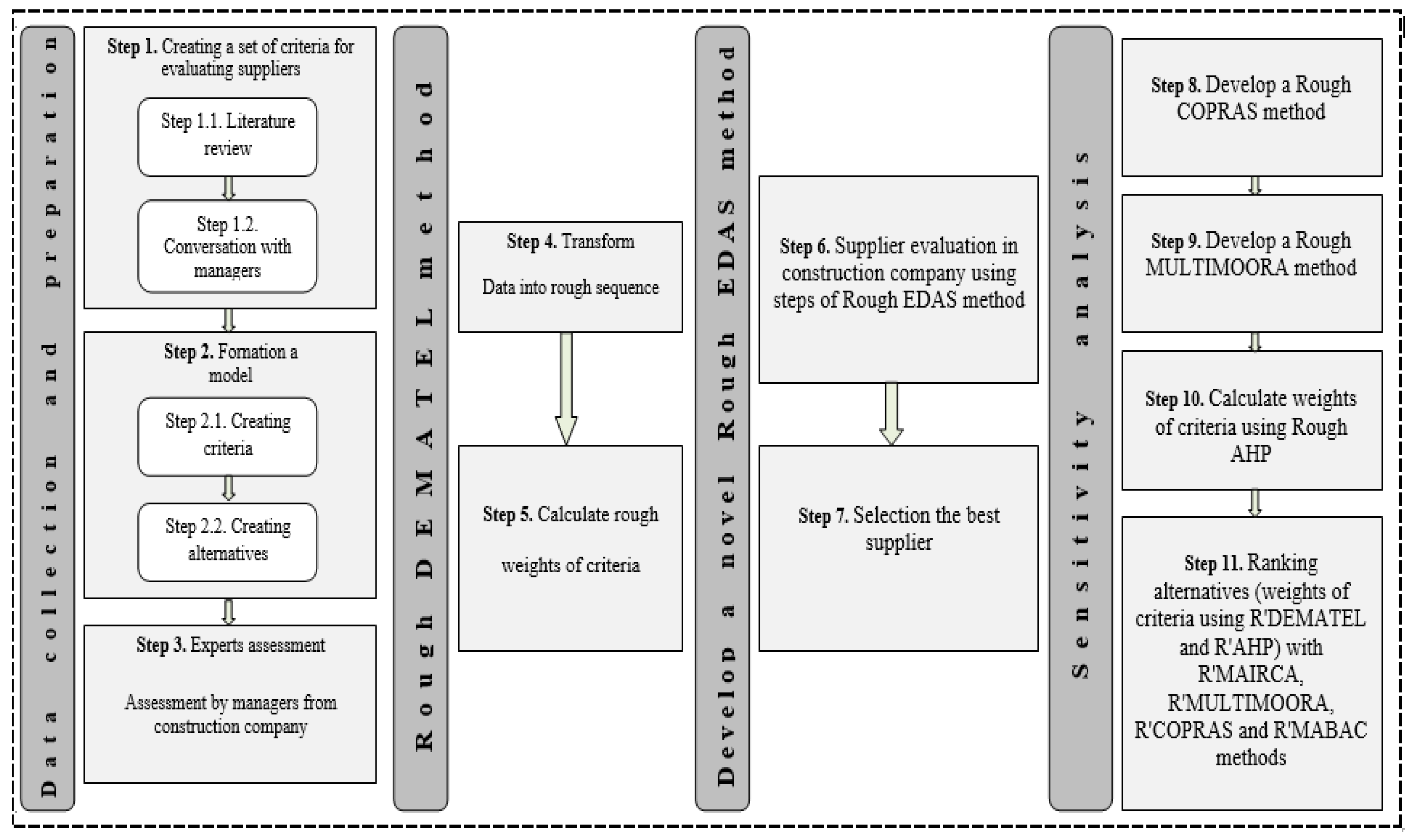
Supplier selection in the construction company was carried out on the basis of nine criteria presented in the Table 1: quality of the material, price of the material, certification of the products, delivery time, reputation, volume discounts, warranty period, reliability, and the method of payments. The second and the fourth criteria (the price of the material and delivery time) are the Expenses criteria, and the others are the Benefit criteria. Figure 1 shows the proposed model for the supplier selection in this study.

Figure 1 shows the proposed model for the supplier selection, which consists of 4 phases and 11 steps. The first phase assumes the collection and preparation of the date in three steps. The first step is defining the set of the criteria for evaluation of the supplier on the basis of the other studies in this field, and an interview with the managers with long-lasting experience on management functions in the supply business. Then, a multi-criteria model has been adopted, consisting of nine criteria and six alternatives evaluated by team of seven experts. The second phase of the model assumes the application of rough DEMATEL method for estimation of the relative weight of the criteria. The steps of this method are presented in detail in section Methods, and the procedure for the weight estimation is described in following. The third and the central phase of this study is development of a new novel Rough EDAS method used for evaluation and the best supplier selection. The last, fourth phase includes sensitivity analysis extended by two additional methods for multi-criteria decision making, COPRAS and MULTIMORA. Comparison of the obtained results and alternative ranges has been performed, applying the above-mentioned two methods, as well with the R’MAICA and R’MABAC, previously extended by rough numbers.

4.1. Estimation of the Criteria Weight by Applying R’DEMATEL Method

In this study, the team of seven experts took part in the process of determination of weight coefficients of criteria. The experts with the minimum of five-year experience in the supply chain management were chosen. After the interview with the experts, the collected data were processed, and the aggregation of the expert opinion was obtained. The collecting of data through the interview with the experts was carried out in the period from March 2017 until June 2017.

Step 1 Expert Analysis of the Factors

In the first step of application of DEMATEL method for the determination of the criteria, experts have used the point scale: 0—no influence, 1—very low influence, 2—low influence, 3—medium influence, 4—high influence, 5—very high influence. After the experts’ evaluation, seven matrices of dimensions 9 × 9 have been constructed, in order to compare the set of the criteria. This is presented in

Table 2. Experts’ comparison of the evaluation criteria.

E1										E2
	C1	C2	C3	C4	C5	C6	C7	C8	C9	C1	C2	C3	C4	C5	C6	C7	C8	C9
C1	0	5	5	5	2	4	4	4	3	0	5	5	4	3	5	4	4	3
C2	4	0	4	2	2	3	5	4	3	4	0	4	4	1	5	5	3	3
C3	4	3	0	3	3	4	2	4	3	4	1	0	5	3	5	3	4	3
C4	4	3	5	0	2	3	3	3	5	4	2	5	0	2	5	3	3	5
C5	5	4	5	4	0	4	5	5	3	5	3	5	5	0	5	5	5	3
C6	4	4	3	3	1	0	2	4	4	4	2	4	4	1	0	2	4	4
C7	4	4	3	4	2	4	0	5	5	4	2	4	5	2	5	0	5	5
C8	3	3	4	2	1	2	2	0	3	4	2	5	4	1	4	2	0	3
C9	3	3	4	2	2	2	3	3	0	3	1	4	3	2	4	3	3	0
…
E6										E7
	C1	C2	C3	C4	C5	C6	C7	C8	C9	C1	C2	C3	C4	C5	C6	C7	C8	C9
C1	0	5	4	4	3	5	5	5	2	0	5	5	4	4	4	4	5	3
C2	4	0	3	2	1	3	4	3	3	4	0	3	4	1	5	5	4	2
C3	5	3	0	3	3	3	2	3	3	4	3	0	5	4	5	2	4	2
C4	3	3	4	0	2	4	3	3	4	3	3	5	0	3	5	3	4	5
C5	3	4	4	4	0	3	4	3	4	5	4	5	5	0	5	5	4	3
C6	4	3	3	3	1	0	2	3	5	3	3	3	4	2	0	2	4	4
C7	5	3	3	4	2	3	0	3	5	4	3	3	5	2	4	0	5	4
C8	4	3	4	2	1	3	1	0	4	3	3	4	4	1	5	2	0	3
C9	3	3	4	2	1	3	3	5	0	2	3	5	3	1	5	3	4	0

.

Step 2 Determination of the matrix of the average response of the experts

On the basis of the response expert matrix (Table 2), matrix of the aggregated sequences of experts is constructed (2). By applying the matrix according to Zhai et al., [109], each of the shown sequences is transformed into rough sequence. So, for the sequence $x_{12}=\left\{5;5;4;4;4;5;5\right\}$ we get:

$$\underset{¯}{Lim}\left(4\right)=4.00,\overline{Lim}\left(4\right)=\frac{1}{7}\left(5+5+4+5+5+4+4\right)=4.57$$

$$\underset{¯}{Lim}\left(5\right)=\frac{1}{7}\left(5+5+4+5+5+4+4\right)=4.57,\overline{Lim}\left(5\right)=5.00$$

$$\underset{¯}{Lim}\left(4\right)=4.00,\overline{Lim}\left(4\right)=\frac{1}{7}\left(5+5+4+5+5+4+4\right)=4.57$$

On the basis of the obtained values, each sequence is transformed into rough sequence:

$$RN(x_{12}^1)=\left[4.57,5.00\right];$$

$$RN(x_{12}^2)=\left[4.57,5.00\right];$$

$$RN(x_{12}^3)=\left[4.00,4.57\right];$$

$$RN(x_{12}^4)=\left[4.00,4.57\right];$$

$$RN(x_{12}^5)=\left[4.00,4.57\right];$$

$$RN(x_{12}^6)=\left[4.57,5.00\right];$$

$$RN(x_{12}^7)=\left[4.57,5.00\right].$$

The obtained rough sequences present the uncertainty of the group of experts, which is the result of nonconformity in the criteria evaluation.

By applying the Expression (3), the averaging of the rough sequences is performed. Therefore, we obtain average rough sequence:

$$RN(z_{12})=\left[\underset{¯}{Lim}(z_{12}),\overline{Lim}(z_{12})\right]=\{\begin{array}{l}\underset{¯}{Lim}(z_{12})=\frac{4.57+4.57+4+4+4+4.57+4.57}{7}=4.33\\ \overline{Lim}(z_{12})=\frac{5+5+4.57+4.57+4.57+5+5}{7}=4.82\end{array}$$

In this way, we get the final rough sequence $RN(z_{12})=\left[4.33,4.82\right]$. The application of the described procedure for the other elements of the matrix of the aggregated sequence of the experts (2) provides the average rough matrix of the average responses (4):

$$Z=\left[\begin{array}{cccccc}\left[0.00,0.00\right]& \left[4.33,4.82\right]& \left[4.33,4.82\right]& \left[4.25,4.76\right]& ,\cdots ,& \left[2.33,2.82\right]\\ \left[3.74,3.98\right]& \left[0.00,0.00\right]& \left[3.18,3.67\right]& \left[2.92,4.08\right]& ,\cdots ,& \left[2.51,2.92\right]\\ \left[4.18,4.67\right]& \left[2.04,3.43\right]& \left[0.00,0.00\right]& \left[3.59,4.65\right]& ,\cdots ,& \left[2.74,2.98\right]\\ \left[3.25,3.76\right]& \left[2.56,3.19\right]& \left[4.67,4.97\right]& \left[0.00,0.00\right]& ,\cdots ,& \left[4.67,4.97\right]\\ \cdots & \cdots & \cdots & \cdots & \ddots & \cdots \\ \left[2.51,2.92\right]& \left[2.01,3.13\right]& \left[4.08,4.49\right]& \left[2.55,3.89\right]& ,\cdots ,& \left[0.00,0.00\right]\end{array}\right]$$

Step 3 Normalization of the group direct relation matrix

On the basis of the matrix Z, the elements of the initial direct-relation matrix are determined (5):

$$Z=\left[\begin{array}{cccccc}\left[0.00,0.00\right]& \left[0.12,0.16\right]& \left[0.12,0.15\right]& \left[0.12,0.15\right]& ,\cdots ,& \left[0.06,0.09\right]\\ \left[0.09,0.12\right]& \left[0.00,0.00\right]& \left[0.09,0.12\right]& \left[0.08,0.13\right]& ,\cdots ,& \left[0.07,0.09\right]\\ \left[0.11,0.15\right]& \left[0.06,0.11\right]& \left[0.00,0.00\right]& \left[0.10,0.15\right]& ,\cdots ,& \left[0.07,0.09\right]\\ \left[0.09,0.12\right]& \left[0.07,0.10\right]& \left[0.13,0.16\right]& \left[0.00,0.00\right]& ,\cdots ,& \left[0.13,0.16\right]\\ \cdots & \cdots & \cdots & \cdots & \ddots & \cdots \\ \left[0.07,0.09\right]& \left[0.06,0.1\right]& \left[0.11,0.14\right]& \left[0.07,0.12\right]& ,\cdots ,& \left[0.00,0.00\right]\end{array}\right]$$

The elements of the matrix Z are obtained from the Expression (6):

$$RN(d_{12})=\frac{RN(z_{12})}{s}=\left[\frac{4.56}{36.71},\frac{4.94}{36.71}\right]=\left[0.12,0.16\right]$$

where the value s is obtained from the Expression (8):

$$\begin{array}{cc}\hfill s& =\max \left[\max \left({\displaystyle {\sum }_{j=1}^n\underset{¯}{Lim}(z_{ij})}\right),\max \left({\displaystyle {\sum }_{j=1}^n\overline{Lim}(z_{ij})}\right)\right]\hfill \\ & =\max \left[\max \left(30.74;24.13;24.88;27.06;31.66;\cdots ;21.31\right),\max \left(35.10;28.76;30.37;30.55;36.71;\cdots ;27.72\right)\right]\hfill \\ & =\max [31.66;36.71]=36.71\hfill \end{array}$$

Step 4 Determination of the total relation matrix

The total relation matrix T (11) of the range 9 × 9 is determined from the expressions (9) and (10):

$$Z=\left[\begin{array}{cccccc}\left[0.242,2.903\right]& \left[0.306,2.814\right]& \left[0.368,3.210\right]& \left[0.344,3.313\right]& ,\cdots ,& \left[0.293,2.851\right]\\ \left[0.277,2.519\right]& \left[0.156,2.225\right]& \left[0.290,2.662\right]& \left[0.266,2.757\right]& ,\cdots ,& \left[0.255,2.387\right]\\ \left[0.303,2.689\right]& \left[0.219,2.461\right]& \left[0.219,2.717\right]& \left[0.289,2.935\right]& ,\cdots ,& \left[0.261,2.527\right]\\ \left[0.294,2.655\right]& \left[0.237,2.444\right]& \left[0.346,2.841\right]& \left[0.211,2.795\right]& ,\cdots ,& \left[0.320,2.568\right]\\ \cdots & \cdots & \cdots & \cdots & \ddots & \cdots \\ \left[0.234,2.4\right]& \left[0.191,2.226\right]& \left[0.286,2.582\right]& \left[0.235,2.648\right]& ,\cdots ,& \left[0.165,2.210\right]\end{array}\right]$$

Step 5 Determination of the sum of the rows and columns of the total relation matrix T

In the total relation matrix T, the sum of the rows and columns is presented by vectors R and C (Expressions (12) and (13)):

$$RN(R_i)=\left[\begin{array}{c}\left[2.740,25.844\right]\\ \left[2.190,21.469\right]\\ \left[2.278,22.797\right]\\ \left[2.424,22.705\right]\\ \left[2.841,27.027\right]\\ \left[2.122,20.699\right]\\ \left[2.522,23.897\right]\\ \left[1.935,19.686\right]\\ \left[1.939,20.628\right]\end{array}\right];RN(C_i)=\left[\begin{array}{c}\left[2.551,23.891\right]\\ \left[2.067,22.051\right]\\ \left[2.779,25.344\right]\\ \left[2.541,26.193\right]\\ \left[1.387,13.850\right]\\ \left[2.477,26.275\right]\\ \left[2.171,19.896\right]\\ \left[2.554,24.467\right]\\ \left[2.464,22.784\right]\end{array}\right]$$

In order to obtain the most reliable cause-and-effect relation between criteria and efficient production in CERD, rough values of vectors R and C are transformed into crisp values by using (14)–(16). By applying the Expression (26), the normalization of the vector R is performed:

$$RN({\hat{R}}_1)=\left[\underset{¯}{Lim}({\hat{R}}_1),\overline{Lim}({\hat{R}}_1)\right]=\{\begin{array}{l}\underset{¯}{Lim}({\hat{R}}_1)=\frac{2.740-1.935}{27.027-1.935}=0.032\\ \overline{Lim}({\hat{R}}_1)=\frac{25.844-2.740}{27.027-1.935}=0.953\end{array}$$

After normalization, by applying (15), a total normalized crisp value is obtained:

$${\beta }_1=\frac{\underset{¯}{Lim}({\hat{R}}_1)\cdot \left\{1-\underset{¯}{Lim}({\hat{R}}_1)\right\}+\overline{Lim}({\hat{R}}_1)\cdot \overline{Lim}({\hat{R}}_1)}{1-\underset{¯}{Lim}({\hat{R}}_1)+\overline{Lim}({\hat{R}}_1)}=\frac{0.032\cdot (1-0.032)+0.953\cdot 0.953}{1-0.032+0.953}=0.489$$

Finally, applying the Expression (16), crisp values of the vector $R_1^{crisp}$ are obtained:

$$R_1^{crisp}=\underset{i}{\min }\left\{\underset{¯}{Lim}(R_i)\right\}+{\beta }_1\cdot \left[\underset{i}{\max }\left\{\overline{Lim}(R_i)\right\}-\underset{i}{\min }\left\{\underset{¯}{Lim}(R_i)\right\}\right]=1.935+0.489\cdot (27.027-1.935)=14.201$$

In the similar way, crisp values of other vectors ($R_i^{crisp}$ and $C_i^{crisp}$) are obtained and shown in

Table 3. Crisp values of vectors $R_i^{crisp}$ and $C_i^{crisp}$.

Criterion	${\mathit{R}}_{\mathit{i}}^{\mathit{c}\mathit{r}\mathit{i}\mathit{s}\mathit{p}}$	${\mathit{C}}_{\mathit{i}}^{\mathit{c}\mathit{r}\mathit{i}\mathit{s}\mathit{p}}$	${\mathit{R}}_{\mathit{i}}^{\mathit{c}\mathit{r}\mathit{i}\mathit{s}\mathit{p}}$+${\mathit{C}}_{\mathit{i}}^{\mathit{c}\mathit{r}\mathit{i}\mathit{s}\mathit{p}}$	${\mathit{R}}_{\mathit{i}}^{\mathit{c}\mathit{r}\mathit{i}\mathit{s}\mathit{p}}$−${\mathit{C}}_{\mathit{i}}^{\mathit{c}\mathit{r}\mathit{i}\mathit{s}\mathit{p}}$
C1	14.201	12.939	27.141	1.262
C2	10.678	11.270	21.948	−0.592
C3	11.663	14.171	25.835	−2.508
C4	11.708	14.628	26.336	−2.920
C5	15.157	5.545	20.702	9.612
C6	10.105	14.642	24.747	−4.538
C7	12.624	9.870	22.495	2.754
C8	9.290	13.360	22.650	−4.070
C9	9.919	12.082	22.000	−2.163

.

Step 6 Determination of the threshold value (α) and creation of the cause-and-effect diagram

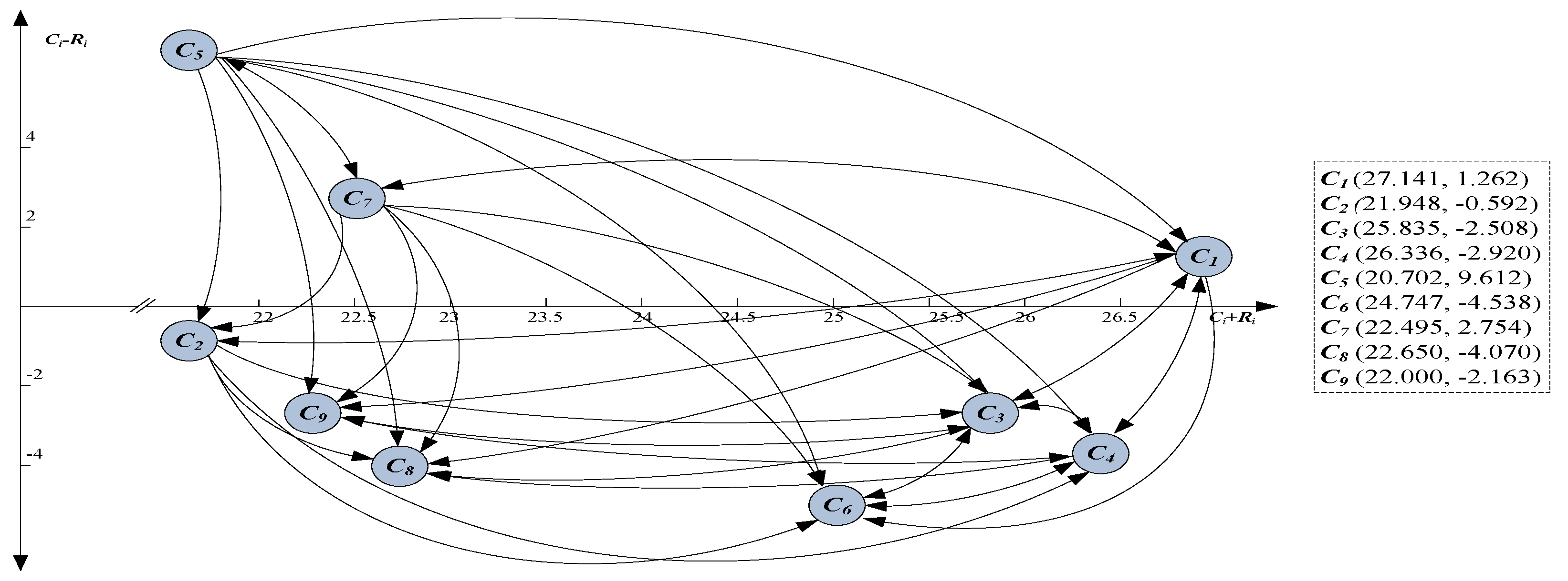
Before determination of the α value, conversion of the elements of the rough matrix T into crisp values was performed using Expressions (14)–(16). After obtaining the crisp values, the value of the α is obtained, $\alpha =1.3935$ (17). Then, α value is used for determination of the cause-and-effect relation between the evaluation criteria. Cause-and-effect relations are presented in CERD (Figure 2). In CERD, the complex relations are visually presented, and provide information about decision making, i.e., which criteria are the most important and how they affect each other. Criteria from the T matrix having values higher than the threshold value, α, are chosen to present cause-and-effect relations.

Step 7 Determination of the weight coefficients of the criteria

The weight coefficients of the criteria are estimated on the basis of the rough values of the vectors $RN(R_i)$ + $RN(C_i)$ and $RN(R_i)$ − $RN(C_i)$ which are defined in

Table 4. Rough values of vectors $RN(R_i)$ and $RN(C_i)$.

Criterion	$\mathit{R}\mathit{N}({\mathit{R}}_{\mathit{i}})$	$\mathit{R}\mathit{N}({\mathit{C}}_{\mathit{i}})$	$\mathit{R}\mathit{N}({\mathit{R}}_{\mathit{i}})$+$\mathit{R}\mathit{N}({\mathit{C}}_{\mathit{i}})$	$\mathit{R}\mathit{N}({\mathit{R}}_{\mathit{i}})$−$\mathit{R}\mathit{N}({\mathit{C}}_{\mathit{i}})$
C1	[2.740, 25.844]	[2.551, 23.891]	[5.292, 49.734]	[−21.150, 23.292]
C2	[2.190, 21.469]	[2.067, 22.051]	[4.257, 43.521]	[−19.861, 19.402]
C3	[2.278, 22.797]	[2.779, 25.344]	[5.057, 48.141]	[−23.067, 20.018]
C4	[2.424, 22.705]	[2.541, 26.193]	[4.964, 48.898]	[−23.770, 20.164]
C5	[2.841, 27.027]	[1.387, 13.850]	[4.228, 40.876]	[−11.008, 25.640]
C6	[2.122, 20.699]	[2.477, 26.275]	[4.599, 46.975]	[−24.153, 18.223]
C7	[2.522, 23.897]	[2.171, 19.896]	[4.693, 43.793]	[−17.374, 21.725]
C8	[1.935, 19.686]	[2.554, 24.467]	[4.488, 44.153]	[−22.532, 17.133]
C9	[1.939, 20.628]	[2.464, 22.784]	[4.403, 43.412]	[−20.845, 18.164]

.

By applying the Expressions (30) and (31), the values of the weight coefficients have been obtained:

$$RN(W_1)=\{\begin{array}{l}\underset{¯}{Lim}(W_1)=\sqrt{{\left(\underset{¯}{Lim}(R_1)+\underset{¯}{Lim}(C_1)\right)}^2+{\left(\underset{¯}{Lim}(R_1)-\overline{Lim}(C_1)\right)}^2}=\sqrt{{\left(2.740+2.551\right)}^2+{\left(2.740-23.891\right)}^2}=21.80\\ \overline{Lim}(W_1)=\sqrt{{\left(\overline{Lim}(R_1)+\overline{Lim}(C_1)\right)}^2+{\left(\overline{Lim}(R_1)-\underset{¯}{Lim}(C_1)\right)}^2}=\sqrt{{\left(25.844+23.891\right)}^2+{\left(25.844-2.551\right)}^2}=54.92\end{array}$$

Thus, we obtain rough weight vectors:

$$RN\left(W_j\right)=\left[\begin{array}{l}\left[21.802,54.918\right]\\ \left[20.313,47.650\right]\\ \left[23.615,52.138\right]\\ \left[24.282,52.893\right]\\ \left[11.792,48.253\right]\\ \left[24.587,50.385\right]\\ \left[17.997,48.885\right]\\ \left[22.975,47.361\right]\\ \left[21.305,47.059\right]\end{array}\right]$$

By applying the Expression (31), additive normalization of the obtained rough weight vectors is performed. In other words, rough weight coefficients are down to the interval [0, 1]:

$$RN(w_1)=\left[\frac{\underset{¯}{Lim}(W_1)}{\underset{j}{\max }\left\{\underset{¯}{Lim}(W_j),\overline{Lim}(W_j)\right\}},\frac{\overline{Lim}(W_1)}{\underset{j}{\max }\left\{\underset{¯}{Lim}(W_j),\overline{Lim}(W_j)\right\}}\right]=\left[\frac{21.80}{54.92},\frac{54.92}{54.92}\right]=\left[0.397,1.00\right]$$

Thus, we obtain rough normalized values of the weight coefficients of the criteria:

$$RN\left(w_j\right)=\left[\begin{array}{l}\left[0.397,1.000\right]\\ \left[0.370,0.868\right]\\ \left[0.430,0.949\right]\\ \left[0.442,0.963\right]\\ \left[0.215,0.879\right]\\ \left[0.448,0.917\right]\\ \left[0.328,0.890\right]\\ \left[0.418,0.862\right]\\ \left[0.388,0.857\right]\end{array}\right]$$

4.2. Supplier Selection Using Rough EDAS Method

After obtaining the weight values of the criteria, the expert team performed evaluation of the alternatives which is shown in

Table 5. Evaluation of the alternatives based on the criteria of seven experts.

E1										E2
	C1	C2	C3	C4	C5	C6	C7	C8	C9	C1	C2	C3	C4	C5	C6	C7	C8	C9
A1	7	1	3	9	1	3	5	3	3	9	1	3	7	9	7	5	9	7
A2	7	3	7	9	3	5	5	5	3	7	3	9	5	7	7	5	7	5
A3	5	7	7	5	7	7	7	5	7	3	9	7	1	5	5	7	5	5
A4	5	3	3	5	7	3	9	5	5	3	7	3	1	5	3	7	5	5
A5	5	9	9	3	7	5	9	5	7	3	9	9	1	5	5	9	5	5
A6	3	7	7	3	5	3	3	3	3	5	7	7	3	5	5	3	5	3
E3										E4
	C1	C2	C3	C4	C5	C6	C7	C8	C9	C1	C2	C3	C4	C5	C6	C7	C8	C9
A1	3	1	1	9	1	3	3	1	3	5	3	3	9	3	1	3	1	1
A2	3	3	5	9	3	5	5	3	1	5	1	5	7	5	3	1	1	3
A3	5	3	3	7	7	3	5	3	3	7	5	5	7	5	5	3	3	5
A4	5	5	1	7	5	5	3	3	5	7	3	3	5	5	3	3	3	3
A5	5	5	5	5	9	7	5	5	5	3	5	7	5	7	7	3	5	5
A6	3	7	3	5	3	3	3	3	7	5	5	5	5	3	5	3	5	7
E5										E6
	C1	C2	C3	C4	C5	C6	C7	C8	C9	C1	C2	C3	C4	C5	C6	C7	C8	C9
A1	7	1	1	9	3	7	5	7	7	5	3	3	9	1	5	3	5	5
A2	7	3	7	9	5	7	5	9	5	5	3	7	9	1	3	5	5	5
A3	5	7	5	5	9	9	7	9	7	5	5	7	7	9	7	5	7	3
A4	5	5	1	5	9	9	9	9	9	3	3	3	7	7	5	3	5	5
A5	5	9	9	1	9	5	9	9	9	7	5	9	7	9	7	5	7	3
A6	3	7	7	3	7	7	3	7	3	5	5	7	7	1	5	3	5	5
E7
	C1	C2	C3	C4	C5	C6	C7	C8	C9
A1	5	3	3	9	1	5	3	5	7
A2	5	3	7	9	1	7	5	5	5
A3	5	5	7	7	9	7	5	7	5
A4	5	3	3	7	7	5	3	5	7
A5	5	5	9	7	9	3	5	7	7
A6	5	5	7	7	1	5	3	5	7

.

Step 1 Conversion of individual matrices into group rough matrix

After computing alternatives by the expert team and converting linguistic values intonumerical, it is necessary to translate individual matrices of all experts into group matrix by applying the matrix according to Zhai et al. [109]. The example of the group matrix elements evaluation is presented in

Table 6. Group rough matrix.

	A1	A2	A3	A4	A5	A6
C1	[4.72, 7.03]	[4.74, 6.37]	[4.48, 5.52]	[4.00, 5.43]	[4.00, 5.43]	[3.65, 4.63]
C2	[1.37, 2.35]	[2.47, 2.96]	[4.72, 7.03]	[3.35, 4.99]	[5.73, 7.69]	[5.65, 6.63]
C3	[2.02, 2.84]	[6.00, 7.43]	[5.01, 6.65]	[2.02, 2.84]	[7.39, 8.83]	[5.39, 6.83]
C4	[8.47, 8.96]	[7.39, 8.83]	[4.37, 6.60]	[4.12, 6.33]	[2.56, 5.67]	[3.72, 5.73]
C5	[1.44, 4.26]	[2.22, 4.95]	[6.27, 8.28]	[5.63, 7.26]	[7.01, 8.65]	[3.05, 5.78]
C6	[3.05, 5.78]	[4.09, 5.91]	[4.97, 7.28]	[3.67, 5.88]	[4.74, 6.37]	[4.00, 5.43]
C7	[3.37, 4.35]	[3.94, 4.92]	[4.74, 6.37]	[3.77, 6.78]	[5.11, 7.78]	[3.00, 3.00]
C8	[2.54, 6.38]	[3.39, 6.61]	[4.22, 6.95]	[4.05, 6.03]	[5.35, 6.99]	[4.00, 5.43]
C9	[3.26, 6.12]	[3.01, 4.65]	[4.09, 5.91]	[4.57, 6.65]	[4.72, 7.03]	[3.93, 6.07]

.

$${\tilde{x}}_{11}=\left\{7,9,3,5,7,5,5\right\}$$

$$\underset{¯}{Lim}\left(3\right)=3.00,\overline{Lim}\left(3\right)=\frac{1}{7}\left(7+9+3+5+7+5+5\right)=5.86$$

$$\underset{¯}{Lim}\left(5\right)=\frac{1}{4}\left(3+5+5+5\right)=4.50, \overline{Lim}\left(5\right)=\frac{1}{6}\left(7+9+5+7+5+5\right)=6.33$$

$$\underset{¯}{Lim}\left(7\right)=\frac{1}{6}\left(7+3+5+7+5+5\right)=5.33, \overline{Lim}\left(7\right)=\frac{1}{3}\left(7+9+7\right)=7.67$$

$$\underset{¯}{Lim}\left(9\right)=\frac{1}{7}\left(7+9+3+5+7+5+5\right)=5.86, \overline{Lim}\left(9\right)=9.00$$

$$RN(x_{11}^1)=RN(x_{11}^5)=\left[5.33;7.67\right];RN(x_{11}^2)=\left[5.86;9.00\right]; RN(x_{11}^3)=\left[3.00;5.86\right]; RN(x_{11}^4)= RN(x_{11}^6)=RN(x_{11}^7)=\left[4.50;6.33\right];$$

$$x_{11}^L=\frac{x_{11}^1+x_{11}^2+x_{11}^s+x_{11}^4+x_{11}^5+x_{11}^6+x_{11}^7}{S}=\frac{5.33+5.86+3.00+4.50+5.33+4.50+4.50}{7}=4.72$$

$$x_{11}^U=\frac{x_{11}^1+x_{11}^2+x_{11}^s+x_{11}^4+x_{11}^5+x_{11}^6+x_{11}^7}{S}=\frac{7.67+9.00+5.86+6.33+7.67+6.33+6.33}{7}=7.03$$

Step 2 Evaluation of the average solution compared to all criteria

The average solution compared to all criteria is obtained after applying Equation (22):

$$RN\left(AV\right)\left[\begin{array}{c}\left[3.66,5.74\right]\\ \left[3.33,5.28\right]\\ \left[3.98,5.90\right]\\ \left[4.38,7.02\right]\\ \left[3.66,6.53\right]\\ \left[3.50,6.11\right]\\ \left[3.42,5.53\right]\\ \left[3.36,6.40\right]\\ \left[3.37,6.07\right]\end{array}\right]$$

Step 3 Evaluation of the positive deviation RN(PDA) and negative deviation RN(NDA) from the average solution compared to all criteria

In order to obtain the values of the positive deviation RN(PDA) (23), shown in

Table 7. Values of the positive deviation from average solution.

PDA	A1		A2		A3		A4		A5		A6
C1	0.18	0.92	0.17	0.74	0.22	0.51	0.30	0.49	0.30	0.49	0.00	0.00
C2	0.19	1.17	0.07	0.84	0.00	0.00	0.32	0.58	0.00	0.00	0.00	0.00
C3	0.00	0.00	0.02	0.87	0.15	0.67	0.00	0.00	0.25	1.22	0.09	0.72
C4	0.00	0.00	0.00	0.00	0.32	0.61	0.28	0.66	0.18	1.02	0.19	0.75
C5	0.00	0.00	0.00	0.00	0.04	1.26	0.14	0.98	0.07	1.36	0.00	0.00
C6	0.00	0.00	0.33	0.69	0.19	1.08	0.00	0.00	0.22	0.82	0.00	0.00
C7	0.00	0.00	0.00	0.00	0.14	0.86	0.32	0.98	0.08	1.28	0.00	0.00
C8	0.00	0.00	0.47	0.96	0.34	1.07	0.37	0.79	0.16	1.08	0.00	0.00
C9	0.00	0.00	0.00	0.00	0.33	0.75	0.25	0.97	0.22	1.09	0.35	0.80

, and the negative deviation RN(NDA) (24) from the average solution RN(AV), shown in

Table 8. Values of the negative deviation from average solution.

NDA	A1		A2		A3		A4		A5		A6
C1	0.00	0.00	0.00	0.00	0.00	0.00	0.00	0.00	0.00	0.00	0.17	0.57
C2	0.00	0.00	0.00	0.00	0.11	1.11	0.00	0.00	0.09	1.31	0.07	0.99
C3	0.19	0.98	0.00	0.00	0.00	0.00	0.19	0.98	0.00	0.00	0.00	0.00
C4	0.21	1.05	0.05	1.02	0.00	0.00	0.00	0.00	0.00	0.00	0.00	0.00
C5	0.09	1.39	0.20	1.18	0.00	0.00	0.00	0.00	0.00	0.00	0.32	0.95
C6	0.37	0.87	0.00	0.00	0.00	0.00	0.39	0.70	0.00	0.00	0.32	0.60
C7	0.17	0.63	0.27	0.47	0.00	0.00	0.00	0.00	0.00	0.00	0.08	0.74
C8	0.47	1.15	0.00	0.00	0.00	0.00	0.00	0.00	0.00	0.00	0.32	0.71
C9	0.45	0.83	0.21	0.91	0.00	0.00	0.00	0.00	0.00	0.00	0.00	0.00

, compared to all criteria, it is necessary to apply the Equations (25)–(31), and take care if criteria belong to the Expenses or Benefit type. The procedure for the Benefit type evaluation is as follows:

First, it is necessary to apply the Equation (25). Since it is the first criterion which belongs to Benefit type and first alternative, it is necessary to calculate the difference between alternative one on criterion one and the average solution for the first criterion:

$$\left[X_{il}^L-A{V}_j^U;X_{il}^U-A{V}_j^L\right]=\left[4.72-5.74;7.03-3.66\right]=\left[-1.02;3.37\right]$$

In this case, the lower limit of the obtained rough number has negative value and it is necessary to apply the Equation (31) and then rough number $\left[-1.02;3.37\right]$ goes to its positive value $\left[1.02;3.37\right]$. After that, it is necessary that the obtained absolute value is divided by the average solution on first criterion (25):

$$\frac{\left[1.02;3.37\right]}{\left[3.66;5.74\right]}=\left[\frac{1.02}{5.74};\frac{3.37}{3.66}\right]=\left[0.18;0.92\right]$$

For example, for the value of alternative one compared to third criterion, evaluating the difference between that value and average solution, both negative values of rough number are obtained (for upper and lower limit).By applying the Equation (29), values of rough number will be equal to zero.

On the other hand, for the value of alternative five compared to third criterion, both positive values of rough number are obtained (for upper and lower limit). And according to the Equation (30), they keep the same value.

Evaluation of the RN(PDA) value for the Expenses type of the criteria is performed in the same way, except that at the beginning, it is necessary to define the deviation of the average solution from the alternative value of the criteria discussed in Equation (27). Evaluation of the RN(NDA) value is performed in the same way, only Equations (26) and (28)–(31) are applied.

Step 4 Weighting of the matrices RN(PDA) and RN(NDA)

By adopting the fourth step of the Rough EDAS method, i.e., Equation (32), the weighted matrix for the positive deviation from the average value VPi is obtained, and is presented in

Table 9. Weighted matrix VPi for the positive deviation.

VPI	A1		A2		A3		A4		A5		A6
C1	0.07	0.92	0.07	0.74	0.09	0.51	0.12	0.49	0.12	0.49	0.00	0.00
C2	0.07	1.02	0.03	0.73	0.00	0.00	0.12	0.50	0.00	0.00	0.00	0.00
C3	0.00	0.00	0.01	0.82	0.07	0.64	0.00	0.00	0.11	1.16	0.04	0.68
C4	0.00	0.00	0.00	0.00	0.14	0.58	0.12	0.64	0.08	0.98	0.09	0.73
C5	0.00	0.00	0.00	0.00	0.01	1.11	0.03	0.86	0.02	1.20	0.00	0.00
C6	0.00	0.00	0.15	0.63	0.08	0.99	0.00	0.00	0.10	0.75	0.00	0.00
C7	0.00	0.00	0.00	0.00	0.05	0.77	0.10	0.88	0.03	1.14	0.00	0.00
C8	0.00	0.00	0.20	0.83	0.14	0.92	0.15	0.68	0.07	0.93	0.00	0.00
C9	0.00	0.00	0.00	0.00	0.13	0.65	0.10	0.83	0.09	0.93	0.14	0.69

.

By applying the Equation (33), weighted matrix for the negative deviation from the average value is obtained and is presented in

Table 10. Weighted matrix VNi for the negative deviation.

VNI	A1		A2		A3		A4		A5		A6
C1	0.00	0.00	0.00	0.00	0.00	0.00	0.00	0.00	0.00	0.00	0.07	0.57
C2	0.00	0.00	0.00	0.00	0.04	0.97	0.00	0.00	0.03	1.14	0.03	0.86
C3	0.08	0.93	0.00	0.00	0.00	0.00	0.08	0.93	0.00	0.00	0.00	0.00
C4	0.09	1.01	0.02	0.98	0.00	0.00	0.00	0.00	0.00	0.00	0.00	0.00
C5	0.02	1.22	0.04	1.03	0.00	0.00	0.00	0.00	0.00	0.00	0.07	0.84
C6	0.17	0.80	0.00	0.00	0.00	0.00	0.17	0.64	0.00	0.00	0.14	0.55
C7	0.06	0.56	0.09	0.41	0.00	0.00	0.00	0.00	0.00	0.00	0.02	0.66
C8	0.20	0.99	0.00	0.00	0.00	0.00	0.00	0.00	0.00	0.00	0.14	0.61
C9	0.18	0.72	0.08	0.78	0.00	0.00	0.00	0.00	0.00	0.00	0.00	0.00

.

Step 5 Determination of the Sum of the Previously Weighted Matrix

By adopting the step five, six, and seven, i.e., the Equations (34)–(38), the final results are obtained and are presented in

Table 11. Results and ranging of the alternatives.

	SPi	SNi	NSPi	NSNi	ASi	Rank
A1	[0.14, 1.94]	[0.79, 6.23]	[0.02, 3.20]	[0.87, −6.89]	−1.40	5
A2	[0.45, 3.76]	[0.24, 3.21]	[0.06, 6.21]	[0.96, −3.07]	2.08	4
A3	[0.70, 6.16]	[0.04, 0.97]	[0.09, 10.17]	[0.99, −0.22]	5.52	2
A4	[0.74, 4.88]	[0.26, 1.57]	[0.10, 8.06]	[0.96, −0.99]	4.07	3
A5	[0.61, 7.57]	[0.03, 1.14]	[0.08, 12.49]	[0.99, −0.44]	6.56	1
A8	[0.26, 2.10]	[0.46, 4.09]	[0.03, 0.28]	[0.93, −4.19]	−1.48	6

. Step 5 summarizes values of the previously weighted matrices RN(SPi) (34), RN(NPi) (35).

$$RN\left(SPi\right)=\left[\begin{array}{c}\left[0.14,1.94\right]\\ \left[0.45,3.76\right]\\ \left[0.70,6.16\right]\\ \left[0.74,4.88\right]\\ \left[0.61,7.57\right]\\ \left[0.26,2.10\right]\end{array}\right];\mathrm{RN}\left(\mathrm{SNi}\right)=\left[\begin{array}{c}\left[0.79,6.23\right]\\ \left[0.24,3.21\right]\\ \left[0.04,0.97\right]\\ \left[0.26,1.57\right]\\ \left[0.03,1.14\right]\\ \left[0.46,4.09\right]\end{array}\right]$$

Step 6  Normalization of the RN(SP) and RN(NP) values for all the alternatives

By applying the Equation (36)

$$RN(NS{P}_1)=\frac{\left[s{p}_1^L;s{p}_1^U\right]}{max\left[s{p}_5^L;s{p}_5^U\right]}=\left[\frac{0.14}{7.67};\frac{1.94}{0.61}\right]=\left[0.02;3.20\right]$$

and (37)

$$RN(NS{N}_1)=1-\frac{\left[s{n}_1^L;s{n}_1^U\right]}{max\left[s{n}_1^L;s{n}_1^U\right]}=1-\left[\frac{0.79}{6.23};\frac{6.23}{0.79}\right]=\left[0.87;-6.89\right]$$

normalized values are obtained, and are presented in Table 11.

Step 7 Estimation of all RN(ASi) alternatives values and their ranging

By applying the Equation (38), the values RN(ASi) are obtained and are presented in Table 11. In the final, seventh step, the ranging towards the falling series of numbers was performed as well. The highest value presents the best solution, whereas the lowest value is the worst solution.

Alternative five, according to the results, presents the best choice.

5. Sensitivity Analysis and Discussion

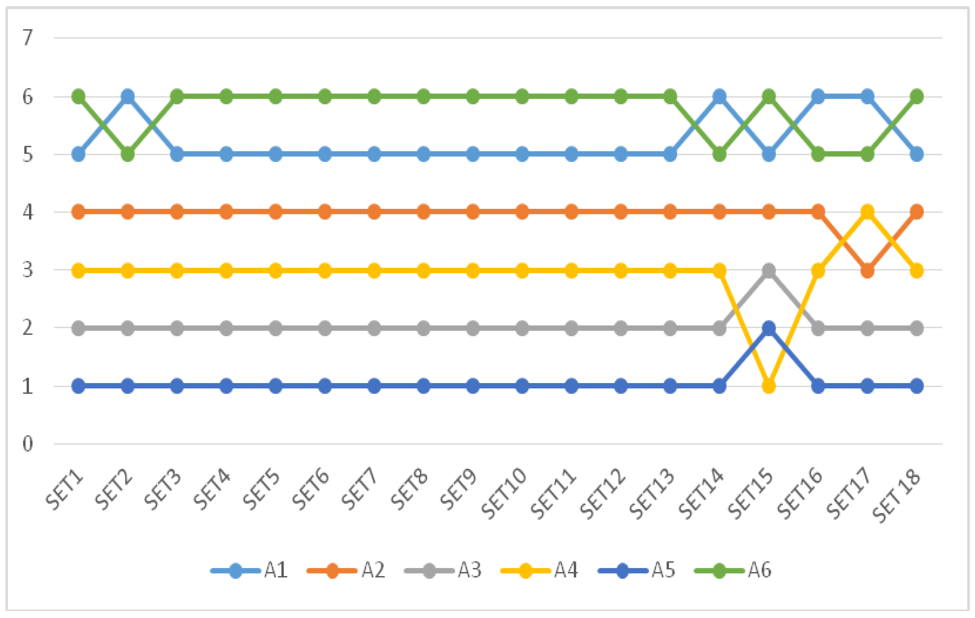
In order to determine the stability of the obtained results, sensitivity analysis has been performed. In the first part, it assumes the change of the criteria weight through 18 different sets. In the first nine sets, the value of each criterion is reduced by 16%, while the value of the rest is increased by 2%, respectively. In the tenth set, the first, the third, and the fourth criteria are reduced by 12%, and the rest are increased by 6%, while in the eleventh set of values, the same criteria are reduced by 24%, and the rest are increased by 12%. Since the ranges of the alternatives have not considerably changed through previously formed sets, the next sets present more significant change of the criteria weigh value expressed in percentage. Thus, in the 12th set, the first, the third, the fourth and the sixth criteria are decreased by 20%, while the remaining five are increased by 16%, while in the 13th set, the first and the fourth criteria are decreased by even 35%, and the rest are decreased by 10%. The second and the seventh criteria in the 14th set are reduced by 28%, while the rest are increased by 8%. The 15th set is based on the five criteria in total, because the first, third, fourth and sixth have been assigned zero values, and the values of the rest of the criteria stay constant. In the 16th set, all criteria have the same importance, while the lower and the upper limit of rough number is also equal. Then the second, the fifth, and the seventh criteria in the 17th set have been assigned zero values, and the rest stay constant. The last, 18th set has the same values of all criteria (assigned maximum value of the first criterion in the basic calculation). In Figure 3, the ranges of the alternatives of all sets have been presented.

In Figure 3, the range of alternatives through formed sets has been presented and, as one can see, alternative five presents the best choice in 17 of the 18 formed scenarios. Only in the 15th set, when the individual criteria are eliminated, does it take the second position. The same is true for alternative two, which takes the third position only in the 17th set, while in other scenarios is in the fourth position. Besides the stability shown in the first part of the sensitivity analysis, the comparison of the proposed model with the other hybrid multi-criteria models has also been performed. The hybrid models used for the comparison of the results are shown in

Table 14. The comparative analysis of the ranges by applying different approaches.

Alternative	R’D-R-MAIRCA			R’D-R-MULTIMOORA			R’D-R-COPRAS			R’D-R-MABAC			R’D-R-EDAS
	Value		Rank	Value		Rank	Value		Rank	Value		Rank	Value		Rank
A1	−0.243	1.540	6	0.778	4.055	6	63.32	83.67	6	−9.508	8.469	6	0.892	−3.690	5
A2	−0.324	1.449	4	0.962	4.392	3	79.70	87.89	3	−9.053	8.875	4	1.021	3.139	4
A3	−0.543	1.394	2	1.059	5.080	2	88.60	93.74	2	−8.779	9.968	2	1.086	9.949	2
A4	−0.402	1.454	3	0.858	4.406	4	78.93	88.10	4	−9.079	9.263	3	1.057	7.073	3
A5	−0.696	1.332	1	1.150	5.402	1	100.00	100.00	1	−8.470	10.73	1	1.075	12.053	1
A6	−0.170	1.463	5	0.933	4.137	5	77.23	78.93	5	−9.123	8.106	5	0.960	−3.913	6
Alternative	R’A-R-MAIRCA			R’A-R-MULTIMOORA			R’A-R-COPRAS			R’A-R-MABAC			R’A-R-EDAS
	Value		Rank	Value		Rank	Value		Rank	Value		Rank	Value		Rank
A1	0.024	0.628	3	0.711	2.103	4	90.72	100.00	3	−2.638	2.919	3	0.759	0.255	5
A2	0.115	0.595	5	0.796	1.991	5	93.58	91.70	5	−2.470	2.466	5	1.056	2.312	4
A3	0.064	0.568	2	0.928	2.320	2	98.60	92.26	2	−2.334	2.721	2	1.205	4.461	2
A4	0.075	0.599	4	0.810	2.151	3	94.25	92.67	4	−2.489	2.668	4	1.148	3.928	3
A5	0.034	0.560	1	0.966	2.420	1	100.00	95.39	1	−2.295	2.872	1	1.195	4.844	1
A6	0.225	0.650	6	0.820	1.982	6	83.13	80.28	6	−2.746	1.915	6	0.879	−1.461	6

* R’D-R-MAIRCA (Rough DEMATEL rough MAIRCA); R’D-R-MULTIMOORA (Rough DEMATEL rough MULTIMOORA); R’D-R-COPRAS (Rough DEMATEL rough COPRAS); R’D-R-EDAS (Rough DEMATEL rough EDAS); R’A-R-MAIRCA (Rough AHP rough MAIRCA); R’A-R-MULTIMOORA (Rough AHP rough MULTIMOORA); R’A-R-COPRAS (Rough AHP rough COPRAS); R’A-R-MABAC (Rough AHP rough MABAC);R’A-R-EDAS (Rough AHP rough EDAS).

. In order to validate the proposed model for determination of the criteria weight, besides R’DEMATEL method, Rough AHP method [123] has been applied as well. AHP model is chosen for the comparison, since this is the method in which literature has already been used for the ranging of alternatives and determination of the criteria weight [109].

For experts’ comparison of criteria sets in Rough AHP method, the same experts as in Rough DEMATEL method participated. After the experts’ evaluation of criteria, by applying Saaty’s scale, seven matrices of comparison of dimensions 9 × 9 were constructed in criteria sets. This is shown in

Table 12. Experts’ comparison of the criteria.

E1										E2
	C1	C2	C3	C4	C5	C6	C7	C8	C9	C1	C2	C3	C4	C5	C6	C7	C8	C9
C1	1	4	9	7	8	3	6	5	2	1	3	8	6	7	2	5	4	2
C2	0.25	1	5	3	4	0.50	3	2	0.33	0.33	1	5	3	4	0.500	3	2	0.33
C3	0.11	0.20	1	0.33	0.50	0.16	0.25	0.33	0.12	0.12	0.20	1	0.33	0.500	0.16	0.25	0.33	0.12
C4	0.14	0.33	3	1	2	0.25	0.50	0.33	0.16	0.16	0.33	3	1	2	0.25	0.500	0.33	0.16
C5	0.12	0.25	2	0.50	1	0.20	0.33	0.25	0.14	0.14	0.25	2	0.500	1	0.20	0.33	0.25	0.14
C6	0.33	2	6	4	5	1	3	3	0.50	0.500	2	6	4	5	1	3	3	0.500
C7	0.16	0.33	4	2	3	0.33	1	0.50	0.25	0.20	0.33	4	2	3	0.33	1	0.500	0.25
C8	0.20	0.50	3	3	4	0.33	2	1	0.33	0.25	0.500	3	3	4	0.33	2	1	0.33
C9	0.50	3	8	6	7	2	4	3	1	0.50	3	8	6	7	2	4	3	1
…
E6										E7
	C1	C2	C3	C4	C5	C6	C7	C8	C9	C1	C2	C3	C4	C5	C6	C7	C8	C9
C1	1	4	9	5	8	3	6	5	2	1	3	8	5	7	2	5	4	3
C2	0.25	1	5	2	4	0.50	3	2	0.33	0.33	1	6	3	4	0.50	4	2	1
C3	0.11	0.20	1	0.25	0.50	0.16	0.25	0.33	0.12	0.12	0.16	1	0.25	0.50	0.16	0.33	0.25	0.20
C4	0.20	0.50	4	1	4	0.33	2	1	0.25	0.20	0.33	4	1	3	0.33	1	0.50	0.33
C5	0.12	0.25	2	0.25	1	0.20	0.33	0.25	0.14	0.14	0.25	2	0.33	1	0.20	0.33	0.25	0.25
C6	0.33	2	6	3	5	1	3	3	0.50	0.50	2	6	3	5	1	3	2	2
C7	0.16	0.33	4	0.50	3	0.33	1	0.50	0.25	0.20	0.25	3	1	3	0.33	1	0.50	0.33
C8	0.20	0.50	3	1	4	0.33	2	1	0.33	0.25	0.50	0.25	2	4	0.50	2	1	0.50
C9	0.50	3	8	4	7	2	4	3	1	0.33	1	5	3	4	0.50	3	2	1

.

By applying the expressions according to Zhai et al., [109], each of presented sequences is transformed in rough sequence. The example of the group matrix elements evaluation is presented in

Table 13. Group rough matrix.

	A1	A2	A3	A4	A5	A6
C1	[1, 1]	[2.78, 3.49]	[7.78, 8.49]	[5.51, 6.22]	[7.08, 7.49]	[2.08, 2.49]
C2	[0.3, 0.38]	[1, 1]	[5.18, 5.99]	[2.78, 3.83]	[4.18, 4.99]	[0.42, 0.63]
C3	[0.12, 0.13]	[0.17, 0.19]	[1, 1]	[0.29, 0.33]	[0.51, 0.63]	[0.16, 0.17]
C4	[0.16, 0.18]	[0.28, 0.38]	[3.08, 3.49]	[1, 1]	[2.18, 2.99]	[0.23, 0.29]
C5	[0.14, 0.14]	[0.2, 0.24]	[1.74, 1.98]	[0.36, 0.47]	[1, 1]	[0.18, 0.20]
C6	[0.42, 0.49]	[1.78, 2.49]	[6.04, 6.53]	[3.53, 4.51]	[5.06, 5.8]	[1, 1]
C7	[0.19, 0.22]	[0.26, 0.32]	[3.74, 3.98]	[1.35, 1.92]	[3.02, 3.26]	[0.31, 0.33]
C8	[0.23, 0.29]	[0.39, 0.49]	[2.27, 2.94]	[2.19, 2.91]	[3.74, 3.98]	[0.34, 0.38]
C9	[0.50, 1.08]	[2.19, 3.52]	[7.17, 8.22]	[4.66, 6.15]	[6.19, 7.45]	[1.34, 2.23]

.

$$\underset{¯}{Lim}\left(2\right)=2.00, \overline{Lim}\left(2\right)=\frac{1}{7}\left(4+3+2+3+3+4+3\right)=3.14$$

$$\underset{¯}{Lim}\left(3\right)=\frac{1}{5}\left(3+2+3+3+3\right)=2.80,\overline{Lim}\left(3\right)=\frac{1}{6}\left(4+3+3+3+4+3\right)=3.33$$

$$\underset{¯}{Lim}\left(4\right)=\frac{1}{7}\left(4+3+2+3+3+4+3\right)=3.14, \overline{Lim}\left(4\right)=4.00$$

$$RN(x_{12}^1)=RN(x_{12}^6)=\left[3.14;4.00\right];RN(x_{12}^2)=RN(x_{12}^4)=RN(x_{12}^5)=RN(x_{12}^7)=\left[2.80;3.33\right]; RN(x_{12}^3)=\left[2.00;3.14\right]$$

$$x_{12}^L=\frac{x_{12}^1+x_{12}^2+x_{12}^s+x_{12}^4+x_{12}^5+x_{12}^6+x_{12}^7}{S}=\frac{3.14+2.80+2.00+2.80+2.80+3.14+2.80}{7}=2.78$$

$$x_{12}^U=\frac{x_{12}^1+x_{12}^2+x_{12}^s+x_{12}^4+x_{12}^5+x_{12}^6+x_{12}^7}{S}=\frac{4.00+3.33+3.14+3.33+3.33+4.00+3.33}{7}=3.49$$

After defining group rough matrix (Table 13), it is necessary to define geometric middle of upper and lower limit of group matrix of criteria, i.e., geometric middle of rows is calculated. From the obtained matrix maximum value, the upper limit is chosen, and all other values are divided by that one. In that way, we obtain the final values of the criteria weight:

$$w_j\left[\begin{array}{c}\left[0.837,1.000\right]\\ \left[0.354,0.462\right]\\ \left[0.066,0.073\right]\\ \left[0.132,0.176\right]\\ \left[0.083,0.093\right]\\ \left[0.495,0.610\right]\\ \left[0.173,0.196\right]\\ \left[0.229,0.269\right]\\ \left[0.636,0.880\right]\end{array}\right]$$

For ranging of alternatives, the following methods were used: R’MAIRCA [104], R’MULTIMOORA (extended in this research), R’COPRAS (extended in this research), R’MABAC [98]. Combining rough AHP and rough DEMATEL, which were used for the evaluation of the criteria weight with R’MAIRCA, R’MULTIMOORA, R’Ctable

OPRAS, R’MABAC and R’EDAS models, ten hybrid models were developed (in total), which are shown in Table 14. The same input data were used for all models which assumes criteria weight obtained from R’DEMATEL and R’AHP, and the same values from the group matrix by R’EDAS method (Table 5).

As already mentioned in Section 3.1 of the paper, DEMATEL method is very suitable for the design and analysis of the structural model. This is achieved by defining the cause-and-effect relation between complex factors [95]. Cause-and-effect relations are obtained on the basis of the total direct and indirect influences transferred from one factor to the other, but also received from the other factors. The implementation of DEMATEL method explores interdependent factors and determines the level of this dependency. The method is based on the graph theory, and it ensures visual planning and problem solving. In this way, the relative factors can be divided into cause-and-effect, in order to gain a better insight into their mutual relations. This also provides a better understanding of the complex structure of this problem, relations between the factors, and relations between the structure level and influence of the factors [99]. Based on all of the above, DEMATEL gives more objective insight into weight coefficient values. Besides, the proposed modification of the DEMATEL using RN makes it possible to take into account doubts that occur during the expert evaluation of criteria, thus bridging the existing gap in the methodology in the treatment of uncertainty based on RN. In Section 3.2, one of the reasons for using EDAS method is given: mathematical apparatus which assumes evaluation of alternatives on the basis of positive and negative deviations from the average solution. Such model presents very important support in making decisions in everyday conflict situations. Therefore, in a very short time, EDAS method has found its way in wide application in engineering and business problems. This method [111] has a number of extensions, and the extension by fuzzy logics [114] is performed exactly in the field of supply chain for supplier selection. Several studies have already been published in different fields, where this method has been applied in its traditional form or some other forms [113,114,115,116,117,118,119,120,121,122]. Besides the mentioned advantages of EDAS method, we can point to additional advantages important for this paper: (1) stability of the solution on change of nature and character of the criteria; (2) provides well-structured analytical frame for ranging of alternatives; (3) the number of steps stays the same no matter of the number of criteria; (4) very useful in the case of large number of alternatives and criteria; (5) applicable for the qualitative and quantitative type of criteria; (6) provides the possibility of the stability analysis of the model regarding weight factor interval change.

Some of the advantages mentioned for the EDAS model are also present in the three other multi-criteria models (MABAC, COPRAS and MULTIMOORA) used for the validation of the research results. According to the research of Pamučar and Ćirović (2015), MABAC, COPRAS and MULTIMOORA belong to the group of multi-criteria models providing stable solutions no matter of change of nature and character of criteria. Besides, they offer: (1) very well structured analytical frame for ranging of alternatives; (2) the number of steps stays the same no matter of the number of criteria; (3) applicable even when the information of certain attributes is missing; (4) provides ranging of alternatives in coordinate scales without normalization process; (5) the possibility of using the limit value for obtaining the preferences; (6) can be used for both qualitative and quantitative type of the criteria and offers the possibility of the stability analysis regarding the weight coefficients change. Taking all this into account, we can conclude that these models are very credible and have wide application in solving a number of multi-criteria problems.

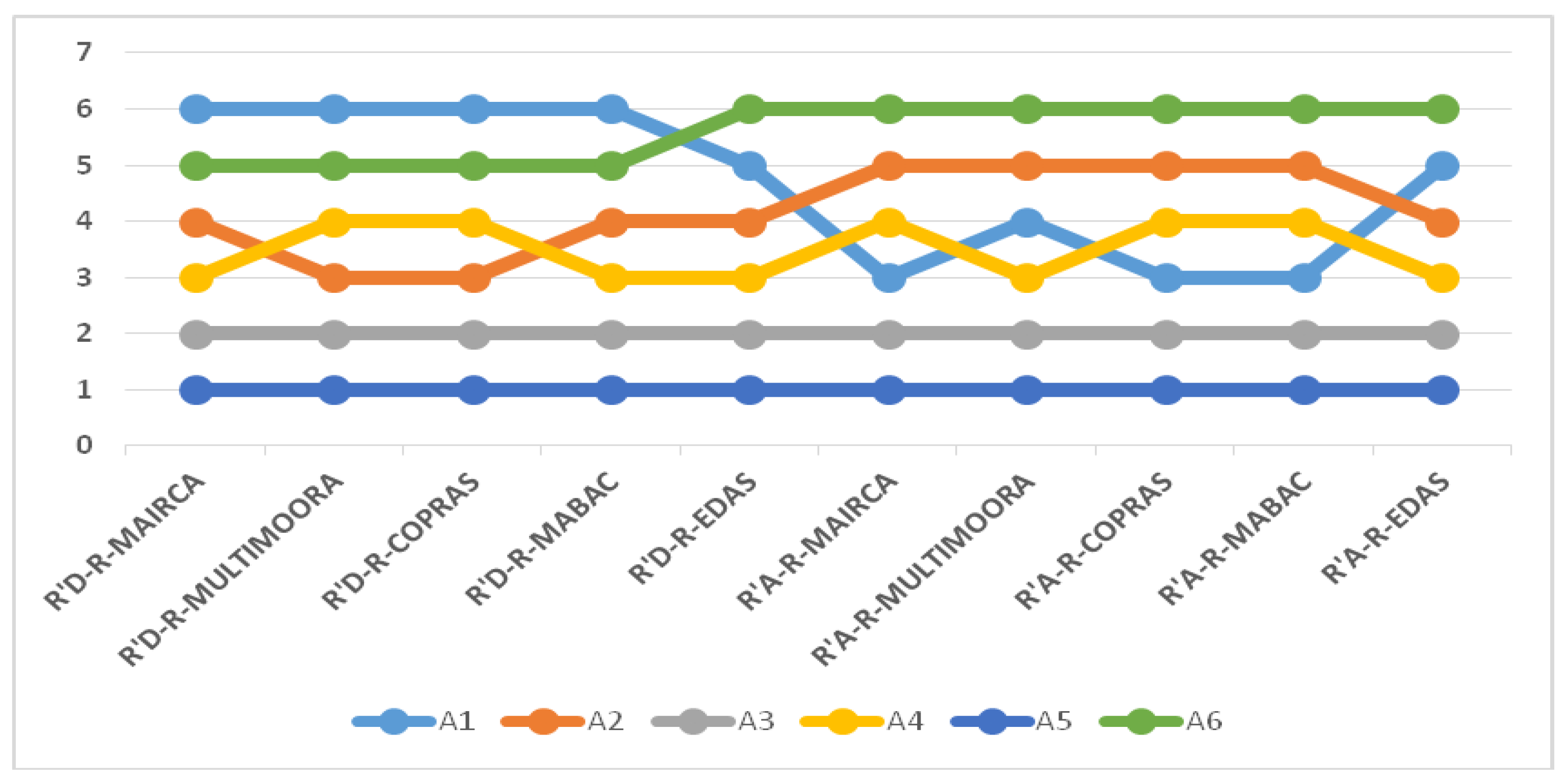
Ranges of alternatives and the values of multi-criteria functions of hybrid models are shown in Table 14. In Figure 4, the changes of the ranges of hybrid models are graphically presented.

Figure 4 shows that alternative five turned out to be the best choice in all 10 models, adequately verifying the proposed model. Alternative A3 is also in all formulated models in the same position—second place. In other alternatives, certain differences are present, as well as dependence from the model applied. Alternative one has the largest variation of all, because it appeared in the last position four times, two times in the fifth position, three times in the third position, and once at the fourth position. Alternative six is, in all models, placed in the fifth or sixth place. Alternative two varies from third to fifth place, and alternative four is in third and fourth place in half of the cases.

For the statistical comparison of the ranges, Spirman coefficient of correlation was used (r_k). The comparison of the ranges was performed through mutual comparison of all 10 hybrid models (

Table 15. Correlation of the ranges of tested models.

Methods	R’D-R-MAI RCA	R’D-R-MULTI MOORA	R’D-R-COP RAS	R’D-R-MA BAC	R’D-R- EDAS	R’A-R-MA IRCA	R’A-R-MULTI MOORA	R’A-R-COP RAS	R’A-R-MA BAC	R’A-R- EDAS	Average
R’D-R-MAIRCA	1.000	0.943	0.943	1.000	0.943	0.657	0.829	0.657	0.657	0.943	0.857
R’D-R-MULTIMOORA	-	1.000	1.000	0.943	0.886	0.600	0.714	0.600	0.600	0.886	0.803
R’D-R-COPRAS	-	-	1.000	0.943	0.886	0.600	0.714	0.600	0.600	0.886	0.779
R’D-R-MABAC	-	-	-	1.000	0.943	0.657	0.829	0.657	0.657	0.943	0.812
R'D-R-EDAS	-	-	-	-	1.000	0.829	0.943	0.829	0.829	1.000	0.905
R’A-R-MAIRCA	-	-	-	-	-	1.000	0.943	1.000	1.000	0.829	0.954
R’A-R-MULTIMOORA	-	-	-	-	-	-	1.000	0.943	0.943	0.943	0.957
R’A-R-COPRAS	-	-	-	-	-	-	-	1.000	1.000	0.829	0.943
R’A-R-MABAC	-	-	-	-	-	-	-	-	1.000	0.829	0.915
R’A-R-EDAS	-	-	-	-	-	-	-	-	-	1.000	1.000
Overall average											0.893

).

Regarding Table 15, one can notice a good correlation of ranges between the considered approaches, since the total average value of r_k is 0.893. The least values of the correlation are obtained by comparison of the ranges R’A-R-MAIRCA model with R’D-R-MAIRCA, R’D-R-MULTIMOORA, R’D-R-COPRAS, and R’D-R-MABAC models, where the obtained values of r_k are 0.657, 0.600, 0.600, and 0.657, respectively. The similar values are also obtained by comparison of R’A-R-COPRAS and R’A-R-MABAC with R’A-R-MAIRCA, R’D-R-MULTIMOORA, R’D-R-COPRAS, and R’D-R-MABAC models. These variations in r_k values arise from application of different approaches for estimation of the weight coefficients. So, the obtained values of the weight coefficients have further influenced the changes in the ranges of the observed models. Therefore, in further analysis, we grouped the models using the same approaches for evaluation of the weight coefficients (R’AHP and R’DEMATEL) and analyzed their mutual correlation. So, for R’AHP model we obtain average r_k = 0.951, while for R’DEMATEL model, we obtain r_k> = 0.962. Taking into account that all values of r_k in the frame of approaches (R’AHP and R’DEMATEL) are considerably higher than 0.8, as well as the average value of r_k is 0.893, we can conclude that there is a very high correlation of the ranges, and that the proposed model has been confirmed.

6. Conclusions

A very important aspect for objective decision making in multi-criteria models is taking into account the uncertainty and imprecision. What often happens are difficulties in presenting information, regarding the attributes of some decisions, through very precise (correct) numerical values. These difficulties are the consequence of certain doubts in decision making, as well as the complexity and uncertainty of many real factors. In this paper, R’DEMATEL–R’EDAS model has been presented. It provides the quantification of the imprecision in group decision making by applying rough numbers. The main idea is based on the interval approach, which assumes application of interval numbers for the presentation of the attribute value. The advantages for the application of rough numbers are numerous. Rough numbers use exclusively intern findings for the presentation of the attribute value. In this way, subjectivity and assumptions are eliminated, since they can considerably influence the attribute value and the final choice of the alternative. In the application of rough numbers, instead of additional/external parameters, only the given data are used. In this way, the uncertainties already present in the date are used, which has considerable influence on the objectivity of the decision-making process. One of the additional advantages of using rough numbers is their application on the sets with small amounts of data, for which traditional statistical models are not suitable.

The application of rough numbers in multi-criteria decision making is presented through the R’DEMATEL and R’EDAS hybrid model. The case study for the evaluation of the supplier in the construction company has been performed. This study shows that rough numbers can be efficiently applied in multi-criteria decision-making models, and can very well handle the doubts appearing in decision making. Another important part of this paper is presenting new R’DEMATEL and R’EDAS models, developed by the authors, which is a contribution to the present MCDM literature. The hybrid R’DEMATEL–R’EDAS model provides objective aggregation of experts’ decisions and takes into account subjectivity and uncertainty present in group decision making. Besides, two new approaches have been introduced based on the combination of MCDM and rough numbers: COPRAS and Rough MULTIMOORA. Development of these models additionally contributes to the literature considering theoretical and practical aspects of multi-criteria techniques.

Besides the general contribution in the field of MCDM, the proposed models help in the field of the supplier selection in the supply chains. It is shown that R’DEMATEL–R’EDAS model enables evaluation of the supplier, despite the imprecision and lack of quantitative information present in decision making process. In this way, the evaluation methodology and the supplier selection in the construction company is improved. To our knowledge, there is no application of such or similar approaches in the literature.

Since our approach is new and not much explored yet, future research will be in the direction of the application of rough numbers in the traditional models for estimation of the weight coefficients (for example, BestWorst Method). Also, one of the future aspects will be the integration of rough numbers in fuzzy numbers, and application of fuzzy-rough numbers in MCDM. This would considerably improve the exploitation of uncertainty and subjectivity always present in the decision-making process.

References

- Soheilirad, S.; Govindan, K.; Mardani, A.; Zavadskas, E.K.; Nilashi, M.; Zakuan, N. Application of data envelopment analysis models in supply chain management: A systematic review and meta-analysis. Ann. Oper. Res. 2017, 1–55. [Google Scholar] [CrossRef]
- Bai, C.; Sarkis, J. Integrating sustainability into supplier selection with grey system and rough set methodologies. Int. J. Prod. Econ. 2010, 124, 252–264. [Google Scholar] [CrossRef]
- Ramanathan, R. Supplier selection problem: Integrating DEA with the approaches of total cost of ownership and AHP. Supply Chain Manag. Int. J. 2007, 12, 258–261. [Google Scholar] [CrossRef]
- Zhong, L.; Yao, L. An ELECTRE I-based multi-criteria group decision making method with interval type-2 fuzzy numbers and its application to supplier selection. Appl. Soft Comput. 2017, 57, 556–576. [Google Scholar] [CrossRef]
- Bai, C.; Sarkis, J. Evaluating supplier development programs with a grey based rough set methodology. Expert Syst. Appl. 2011, 38, 13505–13517. [Google Scholar] [CrossRef]
- Zolfani, S.H.; Chen, I.S.; Rezaeiniya, N.; Tamošaitienė, J. A hybrid MCDM model encompassing AHP and COPRAS-G methods for selecting company supplier in Iran. Technol. Econ. Dev. Econ. 2012, 18, 529–543. [Google Scholar] [CrossRef]
- Cox, A.; Ireland, P. Managing construction supply chains: The common sense approach. Eng. Constr. Archit. Manag. 2002, 9, 409–418. [Google Scholar] [CrossRef]
- Saaty, T.L.; Tran, L.T. On the invalidity of fuzzifying numerical judgments in the Analytic Hierarchy Process. Math. Comput. Model. 2007, 46, 962–975. [Google Scholar] [CrossRef]
- Wang, Y.M.; Luo, Y.; Hua, Z. On the extent analysis method for fuzzy AHP and its applications. Eur. J. Oper. Res. 2008, 186, 735–747. [Google Scholar] [CrossRef]
- Garg, H.; Arora, R. Generalized and group-based generalized intuitionistic fuzzy soft sets with applications in decision-making. Appl. Intell. 2017, 1–14. [Google Scholar] [CrossRef]
- Garg, H. Generalized interaction aggregation operators in intuitionistic fuzzy multiplicative preference environment and their application to multicriteria decision-making. Appl. Intell. 2017, 1–17. [Google Scholar] [CrossRef]
- Garg, H. Some Picture Fuzzy Aggregation Operators and Their Applications to Multicriteria Decision-Making. Arab. J. Sci. Eng. 2017, 42, 5275–5290. [Google Scholar] [CrossRef]
- Garg, H. Confidence levels based Pythagorean fuzzy aggregation operators and its application to decision-making process. Comput. Math. Organ. Theory 2017, 23, 546–571. [Google Scholar] [CrossRef]
- Garg, H.; Arora, R. A nonlinear-programming methodology for multi-attribute decision-making problem with interval-valued intuitionistic fuzzy soft sets information. Appl. Intell. 2017, 1–16. [Google Scholar] [CrossRef]
- Lee, C.; Lee, H.; Seol, H.; Park, Y. Evaluation of new service concepts using rough set theory and group analytic hierarchy process. Expert Syst. Appl. 2012, 39, 3404–3412. [Google Scholar] [CrossRef]
- Garg, H. A new generalized improved score function of interval-valued intuitionistic fuzzy sets and applications in expert systems. Appl. Soft Comput. 2016, 38, 988–999. [Google Scholar] [CrossRef]
- Garg, H. A novel accuracy function under interval-valued pythagorean fuzzy environment for solving multicriteria decision making problem. J. Intell. Fuzzy Syst. 2016, 31, 529–540. [Google Scholar] [CrossRef]
- Garg, H. Generalized Pythagorean Fuzzy Geometric Aggregation Operators Using Einstein t-Norm and t-Conorm for Multicriteria Decision-Making Process. Int. J. Intell. Syst. 2017, 32, 597–630. [Google Scholar] [CrossRef]
- Lima-Junior, F.R.; Carpinetti, L.C.R. A multicriteria approach based on fuzzy QFD for choosing criteria for supplier selection. Comput. Ind. Eng. 2016, 101, 269–285. [Google Scholar] [CrossRef]
- Vonderembse, M.A.; Tracey, M. The impact of supplier selection criteria and supplier involvement on manufacturing performance. J. Supply Chain Manag. 1999, 35, 33–39. [Google Scholar] [CrossRef]
- Dickson, G.W. An analysis of vendor selection and the buying process. J. Purch. 1966, 2, 5–17. [Google Scholar] [CrossRef]
- Teeravaraprug, J. Outsourcing and vendor selection model based on Taguchi loss function. Songklanakarin J. Sci. Technol. 2008, 30, 523–530. [Google Scholar]
- Liao, C.N. Supplier selection project using an integrated Delphi, AHP and Taguchi loss function. Probstat Forum 2010, 3, 118–134. [Google Scholar]
- Parthiban, P.; Zubar, H.A.; Garge, C.P. A multi criteria decision making approach for suppliers selection. Procedia Eng. 2012, 38, 2312–2328. [Google Scholar] [CrossRef]
- Mehralian, G.; Rajabzadeh Gatari, A.; Morakabati, M.; Vatanpour, H. Developing a suitable model for supplier selection based on supply chain risks: An empirical study from Iranian pharmaceutical companies. Iran. J. Pharm. Res. 2012, 11, 209–219. [Google Scholar] [PubMed]
- Cristea, C.; Cristea, M. A multi-criteria decision making approach for supplier selection in the flexible packaging industry. MATEC Web Conf. 2017, 94, 06002. [Google Scholar] [CrossRef]
- Fallahpour, A.; Olugu, E.U.; Musa, S.N. A hybrid model for supplier selection: Integration of AHP and multi expression programming (MEP). Neural Comput. Appl. 2017, 28, 499–504. [Google Scholar] [CrossRef]
- Weber, C.A.; Current, J.R.; Benton, W.C. Vendor selection criteria and methods. Eur. J. Oper. Res. 1991, 50, 2–18. [Google Scholar] [CrossRef]
- Tam, M.C.; Tummala, V.R. An application of the AHP in vendor selection of a telecommunications system. Omega 2001, 29, 171–182. [Google Scholar] [CrossRef]
- Muralidharan, C.; Anantharaman, N.; Deshmukh, S.G. A multi-criteria group decision making model for supplier rating. J. Supply Chain Manag. 2002, 38, 22–33. [Google Scholar] [CrossRef]
- Simpson, P.M.; Siguaw, J.A.; White, S.C. Measuring the performance of suppliers: An analysis of evaluation processes. J. Supply Chain Manag. 2002, 38, 29–41. [Google Scholar] [CrossRef]
- Kannan, V.R.; Choon Tan, K. Buyer-supplier relationships: The impact of supplier selection and buyer-supplier engagement on relationship and firm performance. Int. J. Phys. Distrib. Logist. Manag. 2006, 36, 755–775. [Google Scholar] [CrossRef]
- Gencer, C.; Gürpinar, D. Analytic network process in supplier selection: A case study in an electronic firm. Appl. Math. Model. 2007, 31, 2475–2486. [Google Scholar] [CrossRef]
- Chan, F.T.; Kumar, N. Global supplier development considering risk factors using fuzzy extended AHP-based approach. Omega 2007, 35, 417–431. [Google Scholar] [CrossRef]
- Guo, X.; Yuan, Z.; Tian, B. Supplier selection based on hierarchical potential support vector machine. Expert Syst. Appl. 2009, 36, 6978–6985. [Google Scholar] [CrossRef]
- Lee, A.H. A fuzzy supplier selection model with the consideration of benefits, opportunities, costs and risks. Expert Syst. Appl. 2009, 36, 2879–2893. [Google Scholar] [CrossRef]
- Wang, W.P. A Fuzzy linguistic computing approach to supplier selection. Appl. Math. Model. 2010, 34, 3130–3141. [Google Scholar] [CrossRef]
- Lam, K.C.; Tao, R.; Lam, M.C.K. A material supplier selection model for property developers using fuzzy principal component analysis. Autom. Constr. 2010, 19, 608–618. [Google Scholar] [CrossRef]
- Balezentis, A.; Balezentis, T. An innovative multi-criteria supplier selection based on two-tuple MULTIMOORA and hybrid data. Econ. Comput. Econ. Cybern. Stud. Res. 2011, 45, 37–56. [Google Scholar]
- Raut, R.D.; Bhasin, H.V.; Kamble, S.S. Evaluation of supplier selection criteria by combination of AHP and fuzzy DEMATEL method. Int. J. Bus. Innov. Res. 2011, 5, 359–392. [Google Scholar] [CrossRef]
- Zeydan, M.; Çolpan, C.; Çobanoğlu, C. A combined methodology for supplier selection and performance evaluation. Expert Syst. Appl. 2011, 38, 2741–2751. [Google Scholar] [CrossRef]
- Jamil, N.; Besar, R.; Sim, H.K. A Study of Multicriteria Decision Making for Supplier Selection in Automotive Industry. J. Ind. Eng. 2013, 2013, 841584. [Google Scholar] [CrossRef]
- Kilic, H.S. An integrated approach for supplier selection in multi-item/multi-supplier environment. Appl. Math. Model. 2013, 37, 7752–7763. [Google Scholar] [CrossRef]
- Uygun, Ö.; Kaçamak, H.; Ayşim, G.; Şimşir, F. Supplier selection for automotive industry using multi-criteria decision making techniques. Tojsat Online J. Sci. Technol. 2013, 3, 126–137. [Google Scholar]
- Hruška, R.; Průša, P.; Babić, D. The use of AHP method for selection of supplier. Transport 2014, 29, 195–203. [Google Scholar] [CrossRef]
- Özbek, A. Supplier Selection with Fuzzy. Tojsat J.Econ. Sustain. Dev. 2015, 6, 114–125. [Google Scholar]
- Stević, Ž.; Tanackov, I.; Vasiljević, M.; Novarlić, B.; Stojić, G. An integrated fuzzy AHP and TOPSIS model for supplier evaluation. Serbian J. Manag. 2016, 11, 15–27. [Google Scholar] [CrossRef]
- Tamošaitienė, J.; Zavadskas, E.K.; Šileikaitė, I.; Turskis, Z. A novel hybrid MCDM approach for complicated supply chain management problems in construction. Procedia Eng. 2017, 172, 1137–1145. [Google Scholar] [CrossRef]
- Wang, T.K.; Zhang, Q.; Chong, H.Y.; Wang, X. Integrated Supplier Selection Framework in a Resilient Construction Supply Chain: An Approach via Analytic Hierarchy Process (AHP) and Grey Relational Analysis (GRA). Sustainability 2017, 9, 289. [Google Scholar] [CrossRef]
- Birgün Barla, S. A case study of supplier selection for lean supply by using a mathematical model. Logist. Inf. Manag. 2003, 16, 451–459. [Google Scholar] [CrossRef]
- Wang, G.; Huang, S.H.; Dismukes, J.P. Product-driven supply chain selection using integrated multi-criteria decision-making methodology. Int. J. Prod. Econ. 2004, 91, 1–15. [Google Scholar] [CrossRef]
- Ting, S.C.; Cho, D.I. An integrated approach for supplier selection and purchasing decisions. Supply Chain Manag. 2008, 13, 116–127. [Google Scholar] [CrossRef]
- Sawik, T.; Single, V.S. Multiple objective supplier selection in make to order environment. Omega 2010, 38, 203–212. [Google Scholar] [CrossRef]
- Yücenur, G.N.; Vayvay, Ö.; Demirel, N.Ç. Supplier selection problem in global supply chains by AHP and ANP approaches under fuzzy environment. Int. J. Adv. Manuf. Technol. 2011, 56, 823–833. [Google Scholar] [CrossRef]
- Rezaei, J.; Fahim, P.B.; Tavasszy, L. Supplier selection in the airline retail industry using a funnel methodology: Conjunctive screening method and fuzzy AHP. Expert Syst. Appl. 2014, 41, 8165–8179. [Google Scholar] [CrossRef]
- Büyüközkan, G.; Göçer, F. Application of a new combined intuitionistic fuzzy MCDM approach based on axiomatic design methodology for the supplier selection problem. Appl. Soft Comput. 2017, 52, 1222–1238. [Google Scholar] [CrossRef]
- Hudymáčová, M.; Benková, M.; Pócsová, J.; Škovránek, T. Supplier selection based on multi-criterial AHP method. Acta Montan. Slovaca 2010, 15, 249–255. [Google Scholar]
- Lin, H.T.; Chang, W.L. Order selection and pricing methods using flexible quantity and fuzzy approach for buyer evaluation. Eur. J. Oper. Res. 2008, 187, 415–428. [Google Scholar] [CrossRef]
- Ellram, L.M. The supplier selection decision in strategic partnerships. J. Purch. Mater. Manag. 1990, 26, 8–14. [Google Scholar] [CrossRef]
- Çebi, F.; Bayraktar, D. An integrated approach for supplier selection. Logist. Inf. Manag. 2003, 16, 395–400. [Google Scholar] [CrossRef]
- Zavadskas, E.K.; Vainiūnas, P.; Turskis, Z.; Tamošaitienė, J. Multiple criteria decision support system for assessment of projects managers in construction. Int. J. Inf. Technol. Decis. Mak. 2012, 11, 501–520. [Google Scholar] [CrossRef]
- Antuchevičiene, J.; Zavadskas, E.K.; Zakarevičius, A. Multiple criteria construction management decisions considering relations between criteria. Technol. Econ. Dev. Econ. 2010, 16, 109–125. [Google Scholar] [CrossRef]
- Garg, H. Generalized Intuitionistic Fuzzy Entropy-Based Approach for Solving Multi-attribute Decision-Making Problems with Unknown Attribute Weights. Proc. Natl. Acad. Sci. India Sect. A Phys. Sci. 2017, 1–11. [Google Scholar] [CrossRef]
- Garg, H. Generalized intuitionistic fuzzy interactive geometric interaction operators using Einstein t-norm and t-conorm and their application to decision making. Comput. Ind. Eng. 2017, 101, 53–69. [Google Scholar] [CrossRef]
- Zavadskas, E.K.; Turskis, Z.; Tamošaitiene, J. Risk assessment of construction projects. J. Civ. Eng. Manag. 2010, 16, 33–46. [Google Scholar] [CrossRef]
- Tamošaitienė, J.; Zavadskas, E.K.; Turskis, Z. Multi-criteria risk assessment of a construction project. Procedia Comput. Sci. 2013, 17, 129–133. [Google Scholar] [CrossRef]
- Yao, M.; Minner, S. Review of multi-supplier inventory models in supply chain management: An update. SSRN Electron. J. 2017. [Google Scholar] [CrossRef]
- Izadikhah, M. Group decision making process for supplier selection with TOPSIS method under interval-valued intuitionistic fuzzy numbers. Adv. Fuzzy Syst. 2012, 2012, 407942. [Google Scholar] [CrossRef]
- Eshtehardian, E.; Ghodousi, P.; Bejanpour, A. Using ANP and AHP for the supplier selection in the construction and civil engineering companies; case study of Iranian company. KSCE J. Civ. Eng. 2013, 17, 262–270. [Google Scholar] [CrossRef]
- Fouladgar, M.M.; Yazdani-Chamzini, A.; Zavadskas, E.K.; Haji Moini, S.H. A new hybrid model for evaluating the working strategies: Case study of construction company. Technol. Econ. Dev. Econ. 2012, 18, 164–188. [Google Scholar] [CrossRef]
- Zavadskas, E.K.; Turskis, Z.; Tamosaitiene, J. Selection of construction enterprises management strategy based on the SWOT and multi-criteria analysis. Arch. Civ. Mech. Eng. 2011, 11, 1063–1082. [Google Scholar] [CrossRef]
- Erdogan, S.A.; Šaparauskas, J.; Turskis, Z. Decision Making in Construction Management: AHP and Expert Choice Approach. Procedia Eng. 2017, 172, 270–276. [Google Scholar] [CrossRef]
- Turskis, Z.; Lazauskas, M.; Zavadskas, E.K. Fuzzy multiple criteria assessment of construction site alternatives for non-hazardous waste incineration plant in Vilnius city, applying ARAS-F and AHP methods. J. Environ. Eng. Landsc. Manag. 2012, 20, 110–120. [Google Scholar] [CrossRef]
- Zavadskas, E.K.; Vilutienė, T.; Turskis, Z.; Šaparauskas, J. Multi-criteria analysis of Projects’ performance in construction. Arch. Civ. Mech. Eng. 2014, 14, 114–121. [Google Scholar] [CrossRef]
- Petković, D.; Madić, M.; Radovanović, M.; Gečevska, V. Application of the performance selection index method for solving machining MCDM problems. FU Mech. Eng. 2017, 15, 97–106. [Google Scholar]
- Ristić, M.; Manić, M.; Mišić, D.; Kosanović, M.; Mitković, M. Implant material selection using expert system. FU Mech. Eng. 2017, 15, 133–144. [Google Scholar]
- Stefanović-Marinović, J.; Troha, S.; Milovančević, M. An application of multicriteria optimization to the two-carrier two-speed planetary cear trains. FU Mech. Eng. 2017, 15, 85–95. [Google Scholar]
- Eraslan, E.; Atalay, K.D. A Comparative holistic fuzzy approach for evaluation of the chain performance of suppliers. J. Appl. Math. 2014, 2014, 109821. [Google Scholar] [CrossRef]
- Liao, C.N.; Fu, Y.K.; Wu, L.C. Integrated FAHP, ARAS-F and MSGP methods for green supplier evaluation and selection. Technol. Econ. Dev. Econ. 2016, 22, 651–669. [Google Scholar] [CrossRef]
- Saad, S.M.; Kunhu, N.; Mohamed, A.M. A fuzzy-AHP multi-criteria decision-making model for procurement process. Int. J. Logist. Syst. Manag. 2016, 23, 1–24. [Google Scholar] [CrossRef]
- Bali, S.; Amin, S.S. An analytical framework for supplier evaluation and selection: A multi-criteria decision making approach. Int. J. Adv. Oper. Manag. 2017, 9, 57–72. [Google Scholar]
- Kabi, A.A.; Hussain, M.; Khan, M. Assessment of supplier selection for critical items in public organisations of Abu Dhabi. World Rev. Sci. Technol. Sustain. Dev. 2017, 13, 56–73. [Google Scholar] [CrossRef]
- Secundo, G.; Magarielli, D.; Esposito, E.; Passiante, G. Supporting decision-making in service supplier selection using a hybrid fuzzy extended AHP approach: A case study. Bus. Process Manag. J. 2017, 23, 196–222. [Google Scholar] [CrossRef]
- Yang, J.L.; Tzeng, G.H. An integrated MCDM technique combined with DEMATEL for a novel cluster-weighted with ANP method. Expert Syst. Appl. 2011, 38, 1417–1424. [Google Scholar] [CrossRef]
- Gharakhani, D. The evaluation of supplier selection criteria by fuzzy DEMATEL method. J. Basic Appl. Sci. Res. 2012, 2, 3215–3224. [Google Scholar]
- Ho, L.H.; Feng, S.Y.; Lee, Y.C.; Yen, T.M. Using modified IPA to evaluate supplier’s performance: Multiple regression analysis and DEMATEL approach. Expert Syst. Appl. 2012, 39, 7102–7109. [Google Scholar] [CrossRef]
- Hsu, C.W.; Kuo, T.C.; Chen, S.H.; Hu, A.H. Using DEMATEL to develop a carbon management model of supplier selection in green supply chain management. J. Clean. Prod. 2013, 56, 164–172. [Google Scholar] [CrossRef]
- Lin, R.J. Using fuzzy DEMATEL to evaluate the green supply chain management practices. J. Clean. Prod. 2013, 40, 32–39. [Google Scholar] [CrossRef]
- Mangla, S.; Kumar, P.; Barua, M.K. An evaluation of attribute for improving the green supply chain performance via DEMATEL method. Int. J. Mech. Eng. Robot. Res. 2014, 1, 30–35. [Google Scholar]
- Wu, K.J.; Tseng, M.L.; Chiu, A.S.; Lim, M.K. Achieving competitive advantage through supply chain agility under uncertainty: A novel multi-criteria decision-making structure. Int. J. Prod. Econ. 2017, 190, 96–107. [Google Scholar] [CrossRef]
- Chang, B.; Chang, C.W.; Wu, C.H. Fuzzy DEMATEL method for developing supplier selection criteria. Expert Syst. Appl. 2011, 38, 1850–1858. [Google Scholar] [CrossRef]
- Iirajpour, A.; Hajimirza, M.; Alavi, M.G.; Kazemi, S. Identification and evaluation of the most effective factors in green supplier selection using DEMATEL method. J. Basic Appl. Sci. Res. 2012, 2, 4485–4493. [Google Scholar]
- Sarkar, S.; Lakha, V.; Ansari, I.; Maiti, J. Supplier Selection in Uncertain Environment: A Fuzzy MCDM Approach. In Proceedings of the First International Conference on Intelligent Computing and Communication; Springer; Singapore, 2017; pp. 257–266. [Google Scholar]
- Song, W.; Ming, X.; Wu, Z.; Zhu, B. A rough TOPSIS approach for failure mode and effects analysis in uncertain environments. Qual. Reliab. Eng. Int. 2014, 30, 473–486. [Google Scholar] [CrossRef]
- Pamučar, D.; Ćirović, G. The selection of transport and handling resources in logistics centers using Multi-Attributive Border Approximation area Comparison (MABAC). Expert Syst. Appl. 2015, 42, 3016–3028. [Google Scholar] [CrossRef]
- Gigović, L.; Pamučar, D.; Božanić, D.; Ljubojević, S. Application of the GIS-DANP-MABAC multi-criteria model for selecting the location of wind farms: A case study of Vojvodina, Serbia. Renew. Energy 2017, 103, 501–521. [Google Scholar] [CrossRef]
- Pamučar, D.; Petrović, I.; Ćirović, G. Modification of the Best-Worst and MABAC methods: A novel approach based on interval-valued fuzzy-rough numbers. Expert Syst. Appl. 2017, 91, 89–106. [Google Scholar] [CrossRef]
- Roy, J.; Chatterjee, K.; Bandhopadhyay, A.; Kar, S. Evaluation and selection of Medical Tourism sites: A rough AHP based MABAC approach. arXiv, 2016; arXiv:1606.08962. [Google Scholar]
- Gigović, L.; Pamučar, D.; Bajić, Z.; Drobnjak, S. Application of GIS-Interval Rough AHP Methodology for Flood Hazard Mapping in Urban Areas. Water 2017, 9, 360. [Google Scholar] [CrossRef]
- Khoo, L.-P.; Zhai, L.-Y. A prototype genetic algorithm enhanced rough set-based rule induction system. Comput. Ind. 2001, 46, 95–106. [Google Scholar] [CrossRef]
- Zou, Z.; Tseng, T.L.B.; Sohn, H.; Song, G.; Gutierrez, R. A rough set based approach to distributor selection in supply chain management. Expert Syst. Appl. 2011, 38, 106–115. [Google Scholar] [CrossRef]
- Nauman, M.; Nouman, A.; Yao, J.T. A three-way decision making approach to malware analysis using probabilistic rough sets. Inf. Sci. 2016, 374, 193–209. [Google Scholar] [CrossRef]
- Liang, D.; Xu, Y.; Liu, D. Three-way decisions with intuitionistic fuzzy decision-theoretic rough sets based on point operators. Inf. Sci. 2017, 375, 183–201. [Google Scholar] [CrossRef]
- Pamučar, D.; Mihajlović, M.; Obradović, R.; Atanasković, P. Novel approach to group multi-criteria decision making based on interval rough numbers: Hybrid DEMATEL-ANP-MAIRCA model. Expert Syst. Appl. 2017, 88, 58–80. [Google Scholar] [CrossRef]
- Tiwari, V.; Jain, P.K.; Tandon, P. Product design concept evaluation using rough sets and VIKOR method. Adv. Eng. Inf. 2016, 30, 16–25. [Google Scholar] [CrossRef]
- Shidpour, H.; Cunha, C.D.; Bernard, A. Group multi-criteria design concept evaluation using combined rough set theory and fuzzy set theory. Expert Syst. Appl. 2016, 64, 633–644. [Google Scholar] [CrossRef]
- Chai, J.; Liu, J.N. A novel believable rough set approach for supplier selection. Expert Syst. Appl. 2014, 41, 92–104. [Google Scholar] [CrossRef]
- Zhu, G.N.; Hu, J.; Qi, J.; Gu, C.C.; Peng, J.H. An integrated AHP and VIKOR for design concept evaluation based on rough number. Adv. Eng. Inf. 2015, 29, 408–418. [Google Scholar] [CrossRef]
- Zhai, L.Y.; Khoo, L.P.; Zhong, Z.W. A rough set based QFD approach to the management of imprecise design information in product development. Adv. Eng. Inf. 2009, 23, 222–228. [Google Scholar] [CrossRef]
- Gigović, L.; Pamučar, D.; Lukić, D.; Marković, S. Application of the GIS-Fuzzy DEMATEL MCDA model for ecotourism development site evaluation: A case study of “Dunavski ključ”, Serbia. Land Use Policy 2016, 58, 348–365. [Google Scholar] [CrossRef]
- Keshavarz Ghorabaee, M.; Zavadskas, E.K.; Olfat, L.; Turskis, Z. Multi-Criteria Inventory Classification Using a New Method of Evaluation Based on Distance from Average Solution (EDAS). Informatica 2015, 26, 435–451. [Google Scholar] [CrossRef]
- Keshavarz Ghorabaee, M.; Zavadskas, E.K.; Amiri, M.; Turskis, Z. Extended EDAS Method for Fuzzy Multi-criteria Decision-making: An Application to Supplier Selection. Int. J. Comput. Commun. Control 2016, 11, 358–371. [Google Scholar] [CrossRef]
- Turskis, Z.; Juodagalvienė, B. A novel hybrid multi-criteria decision-making model to assess a stairs shape for dwelling houses. J. Civ. Eng. Manag. 2016, 22, 1078–1087. [Google Scholar] [CrossRef]
- Stević, Ž.; Tanackov, I.; Vasiljević, M.; Vesković, S. Evaluation in logistics using combined AHP and EDAS method. In Proceedings of the XLIII International Symposium on Operational Research, Belgrade, Serbia, 20–23 September 2016; pp. 309–313. [Google Scholar]
- Keshavarz Ghorabaee, M.; Amiri, M.; Olfat, L.; Khatami Firouzabadi, S.A. Designing a multi-product multi-period supply chain network with reverse logistics and multiple objectives under uncertainty. Technol. Econ. Dev. Econ. 2017, 23, 520–548. [Google Scholar] [CrossRef]
- Kahraman, C.; Keshavarz Ghorabaee, M.; Zavadskas, E.K.; Cevik Onar, S.; Yazdani, M.; Oztaysi, B. Intuitionistic fuzzy EDAS method: An application to solid waste disposal site selection. J. Environ. Eng. Landsc. Manag. 2017, 25, 1–12. [Google Scholar] [CrossRef]
- Keshavarz Ghorabaee, M.; Amiri, M.; Zavadskas, E.K.; Turskis, Z. Multi-criteria group decision-making using an extended EDAS method with interval type-2 fuzzy sets. E+M Ekon. Manag. 2017, 20, 48–68. [Google Scholar]
- Ecer, F. Third-party logistics (3PLs) provider selection via Fuzzy AHP and EDAS integrated model. Technol. Econ. Dev. Econ. 2017, 1–20. [Google Scholar] [CrossRef]
- Peng, X.; Liu, C. Algorithms for neutrosophic soft decision making based on EDAS, new similarity measure and level soft set. J. Intell. Fuzzy Syst. 2017, 32, 955–968. [Google Scholar] [CrossRef]
- Keshavarz Ghorabaee, M.; Amiri, M.; Zavadskas, E.K.; Turskis, Z.; Antucheviciene, J. A new hybrid simulation-based assignment approach for evaluating airlines with multiple service quality criteria. J. Air Transp. Manag. 2017, 63, 45–60. [Google Scholar] [CrossRef]
- Zavadskas, E.K.; Cavallaro, F.; Podvezko, V.; Ubarte, I.; Kaklauskas, A. MCDM Assessment of a Healthy and Safe Built Environment According to Sustainable Development Principles: A Practical Neighborhood Approach in Vilnius. Sustainability 2017, 9, 702. [Google Scholar] [CrossRef]
- Trinkūnienė, E.; Podvezko, V.; Zavadskas, E.K.; Jokšienė, I.; Vinogradova, I.; Trinkūnas, V. Evaluation of quality assurance in contractor contracts by multi-attribute decision-making methods. Econ. Res.-Ekon. Istraž. 2017, 30, 1152–1180. [Google Scholar] [CrossRef]
- Song, W.; Ming, X.; Wu, Z. An integrated rough number-based approach to design concept evaluation under subjective environments. J. Eng. Des. 2013, 24, 320–341. [Google Scholar] [CrossRef]
Figure 1.
Proposed model for the supplier selection.
Figure 2.
Cause-and-effect relations between criteria—CERD.
Figure 3.
Ranking of alternatives through the scenario.
Figure 4.
Alternative ranges in combination of R’DEMATEL and R’AHP.