Time Series Seasonal Analysis Based on Fuzzy Transforms

Abstract

We define a new seasonal forecasting method based on fuzzy transforms. We use the best interpolating polynomial for extracting the trend of the time series and generate the inverse fuzzy transform on each seasonal subset of the universe of discourse for predicting the value of an assigned output. In the first example, we use the daily weather dataset of the municipality of Naples (Italy) starting from data collected from 2003 to 2015 making predictions on mean temperature, max temperature and min temperature, all considered daily. In the second example, we use the daily mean temperature measured at the weather station “Chiavari Caperana” in the Liguria Italian Region. We compare the results with our method, the average seasonal variation, Auto Regressive Integrated Moving Average (ARIMA) and the usual fuzzy transforms concluding that the best results are obtained under our approach in both examples. In addition, the comparison results show that, for seasonal time series that have no consistent irregular variations, the performance obtained with our method is comparable with the ones obtained using Support Vector Machine- and Artificial Neural Networks-based models.

1. Introduction

Time series forecasting methods are quantitative techniques that analyze historical data of a variable for predicting its values. Traditional forecasting methods [1,2,3,4,5,6,7] use statistical techniques to estimate the future trend of a variable starting from numerical datasets. Many time series data contain seasonal patterns that have regular, repetitive and predictable changes that happen sequentially in a period of time which could be a year, a season, a month, a week, etc.

Different approaches have been developed to deal with trend and seasonal time series. Traditional approaches, such the moving average method, additive and multiplicative models, Holt-Winters exponential smoothing, etc. [3,4,5,7], use statistical methods for removing the seasonal components: they decompose the series into trend, seasonal, cyclical and irregular components [8]. Other statistical approaches are based on the Box–Jenkins model, called Autoregressive Integrated Moving Average (ARIMA) [3,5,7,9]. In the first phase of ARIMA, an auto-correlation analysis is performed for verifying if the series is non-stationary. Then, the series is transformed into a stationary series formed by the differences between the value at the actual moment and the value at the previous moment.

The main limitation of the seasonal ARIMA model is the fact that the process is considered to be linear. Many soft computing models have been presented in the literature for capturing nonlinear characteristics in seasonal time series, e.g., Support Vector Machine (SVM) [10,11] used for wind speed prediction [12], air quality forecasting [13], and rainfall forecasting [14]. SVM utilizes a kernel function to transform the input variables into a multi-dimensional feature space, and then the Lagrange multipliers are used for finding the best hyperplane to model the data in the feature space. The main advantage of an SVM method is that that the solution is unique and there are no risk to move towards local minima, but some problems remain as the choice of the kernel parameters which influences the structure of the feature space, affecting the final solution. Another method is based on an Artificial Neural Network (ANN) [8,15,16,17]. The most widely used ANN architectures for forecasting problems are given by multi-layer Feed Forward Network (FNN) architectures [18,19], where the input nodes are given by the successive observations of the time series; that is, target y_t is a function of the values y_t−1, y_t−2, …, y_t−p, where p is the number of input nodes.

A variation of FNN is the Time Lagged Neural Network (TLNN) architecture [20,21], where the input nodes are the time series values at some particular lags. For example, in a time series having the month as seasonal period, the neural network used for forecasting the parameter value at the time t can contain input nodes corresponding to the lagged values at the time t − 1, t − 2, .., t − 12. The key point is that an ANN can be considered a nonlinear auto-regression model. ANNs are inherently nonlinear and can accurately model complex characteristics in data patterns with respect to linear approaches such as ARIMA models. One of the main problems in the ANN forecasting models is the selection of appropriate network parameters. This operation is crucial since it strongly affects the final results. Furthermore, the presence of a high number of network parameters in the model can produce overtraining of data, giving rise to incorrect forecasting solutions.

To reduce the problems present in the SVM and ANN approaches, some authors have recently developed some hybrid models, e.g., genetic algorithms and tabu search (GA/TS) [11] and the Modified Firefly Algorithm (MFA).

In [22], a Discrete Wavelet Transform (DWT) algorithm is used to decompose the time series into linear and nonlinear components. Afterwards, the ARIMA and the ANN models are used to forecasting separately the two components.

In [23], the authors present four seasonal forecasting models: an adaptive ANN model that uses a genetic algorithm for evolving the ANN topology and the back-propagation parameter called ADANN (Automatic Design of Artificial Neural Networks), a SVM seasonal forecasting model and two hybrid ANN and SVM models based on linguistic fuzzy rules. The authors compare the four methods with the traditional ARIMA method, showing that the results under the four methods are comparable with the ones obtained using ARIMA. The best results are obtained by using the ADANN algorithm based on linguistic fuzzy rules but ANN-based methods are complex to manage and require more computational effort.

Various fuzzy modeling approaches are proposed in literature and applied in different fields for data analysis and knowledge exploring (for examples, see [24,25,26,27]).

To overcome the high computational complexity and the heavy dependence on the input parameters of the ANN models, a soft computing forecasting method based on fuzzy transforms [28] (for short, F-transforms) is presented in [29]. This method was applied to the North Atlantic Oscillation (NAO) data time series. The results are better than the ones obtained using the well known Wang–Mendel method [30] and Local Linear Wavelet Neural Network (LLWNN) techniques.

F-transforms are a powerful flexible method to be applied in various domains such as image compression [31], detection of attribute dependencies in data analysis [32] and extraction of the trend cycle of time series [33].

Strictly speaking, in [29], a forecasting index is calculated with respect to the data of the training set: if this index is smaller than or equal to an assigned threshold, the algorithm is stopped; otherwise, it is iterated by taking a finer fuzzy partition of the variable domain.

When a fuzzy partition is settled, the algorithm controls that the training dataset is sufficiently dense with respect to the fuzzy partition; that is, each fuzzy set of the fuzzy partition has at least a non-zero membership degree in some point.

Here, we give a forecasting method based on F-transforms for seasonal time series analysis called Time Series Seasonal F-transform (TSSF). We give a partition of the time series dataset into seasonal pattern components. A seasonal pattern is related to a fixed period of the time series fluctuations: the seasonality is set on a fixed period such as year, month, week, etc. In the TSSF model, we assume that the different components affect the time series. We use the best polynomial fit for estimating the trend of the time series. After de-trending the data by subtracting the trend from the time series dataset, we find a fuzzy partition of the dataset into seasonal subsets to which we apply the F-transforms by checking that the chosen partition is optimal for the density of the training data. In [29,32], the authors have developed this process: in particular, four forecasting indexes are proposed for assessing the quality of the results: Mean Absolute Deviation (MAD), Mean Absolute Percentage Error (MAPE), Root Mean Square Error (RMSE) and Mean Absolute Deviation Mean (MADMEAN). An optimal fuzzy partition is found by calculating the corresponding RMSE and MADMEAN: if at least one of the two indices does not exceed a respective threshold, then the process stops and the given fuzzy partition is considered optimal.

1.1 TSSF Method for Forecasting Analysis

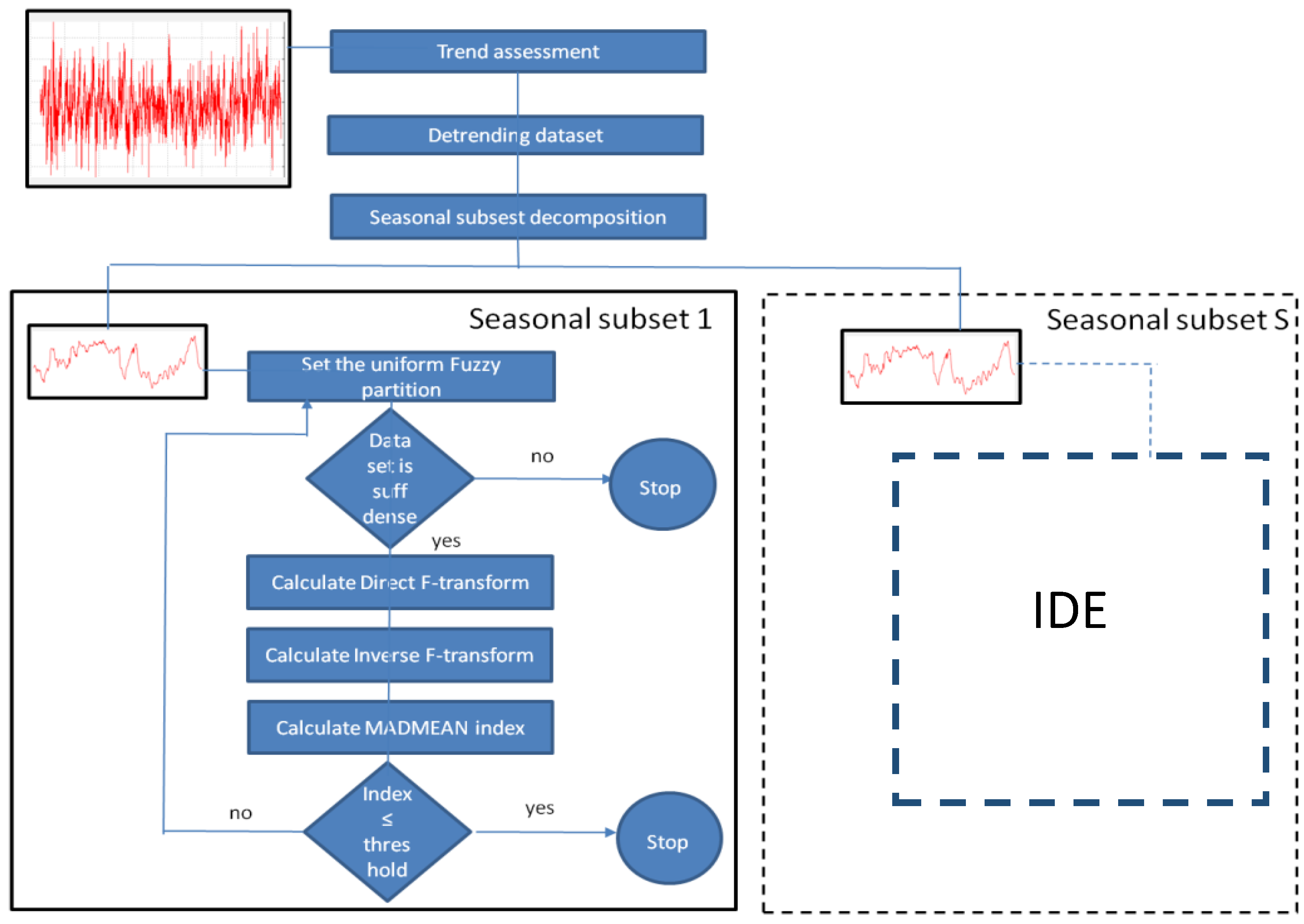
In the TSSF method, we essentially adopt the same procedure, but we prefer to use the MADMEAN index because this index is more robust than other forecasting indexes, as proven in [34]. We emphasize that the dimension of the optimal fuzzy partition can vary with the seasonal subset. In Figure 1, the TSSF method is synthetized in detail.

In the assessment phase, the best polynomial fit is applied for determining the trend in the training data. After de-trending the dataset, the time series is decomposed into S seasonal subsets to which the F-transform forecasting iterative method is applied. Initially, a coarse grained uniform fuzzy partition is fixed. If the subset is not sufficiently dense with respect to the fuzzy partition, the F-transform sub-process applied on the seasonal subset stops, else the MADMEAN index is calculated and, if it is greater than an assigned threshold, the F-transform sub-process is iterated considering a finer uniform fuzzy partition. The output is given by the inverse F-transforms obtained for each seasonal subset at the end of the corresponding sub-process.

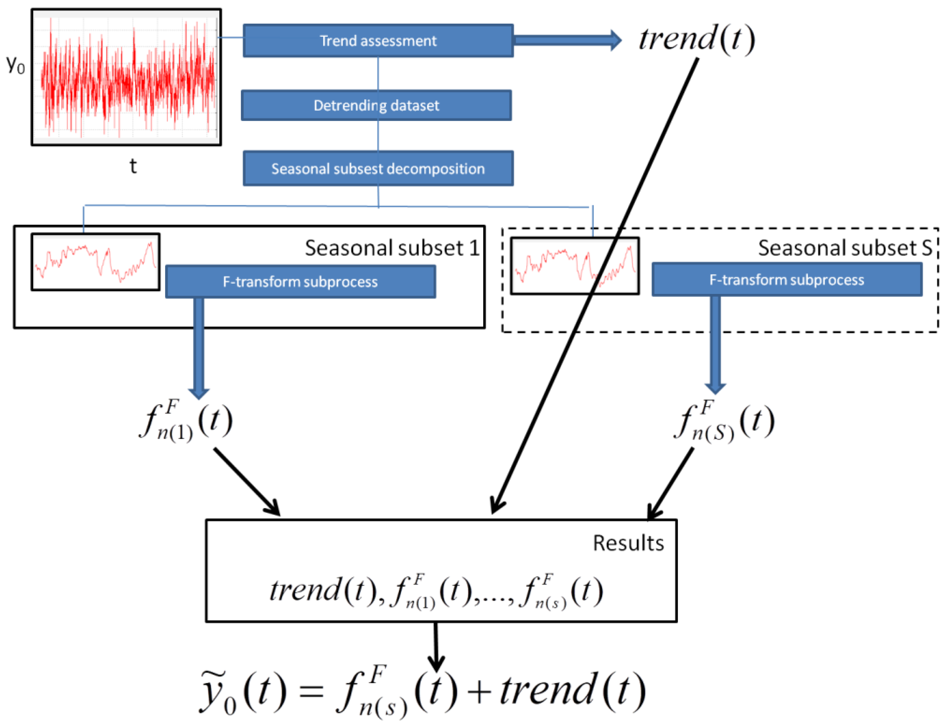
To forecast a value of a parameter y₀ at the time t, we calculate the sth seasonal subset of cardinality n(s), in which the time t is inserted. Then, we consider the sth inverse F-transform $f_{n(s)}^F(t)$. The forecasted value of the parameter is given by the formula $f_{n(s)}^F(t)+trend(t)$, where trend(t) is the value of the polynomial trend at the time t. Figure 2 illustrates the application of the TSSF for forecasting analysis.

For sake of completeness, we recall the concept of F-transform in Section 2. Section 3 contains the F-transform-based prediction method. In Section 4, we describe our TSSF method applied on the climate dataset of Naples (Italy) (www.ilmeteo.it/portale/archivio-meteo/Napoli) whose results are given in Section 5 that contain also comparisons with average seasonal variation, ARIMA and the traditional prediction F-transform methods. Section 6 reports the conclusions.

2. Direct and Inverse F-Transform

Following the definitions and notations of [28], let n ≥ 2 and x₁, x₂, …, x_n be points of [a,b], called nodes, such that x₁ = a < x₂ < … < x_n = b. The family of fuzzy sets A₁, …, A_n: [a,b] → [0,1], called basic functions, is a fuzzy partition of [a,b] if the following hold:

-

A_i(x_i) = 1 for every i =1,2, …,n;

-

A_i(x) = 0 if x $\notin$ [x_i−1,x_i+1] for i = 2, …,n − 1;

-

A_i(x) is a continuous function on [a,b];

-

A_i(x) strictly increases on [x_i−1, x_i] for i = 2, …, n and strictly decreases on [x_i,x_i+1] for i = 1, …, n − 1;

-

A₁(x) +…+ A_n(x) = 1 for every x $\in$ [a,b].

The fuzzy sets {A₁(x),…,A_n(x)} form an uniform fuzzy partition if n ≥ 3 and x_i = a + h∙(i − 1), where h = (b − a)/(n − 1) and i = 1, 2, …, n (that is the nodes are equidistant);

-

A_i(x_i − x) = A_i(x_i + x) for every x $\in$ [0,h] and i = 2, …, n − 1;

-

A_i+1(x) = A_i(x − h) for every x $\in$ [x_i, x_i+1] and i = 1,2, …, n − 1.

Here, we are only interested in the discrete case, i.e., for functions f defined on the set P of points p₁, ..., p_m of [a,b]. If P is sufficiently dense with respect to the given partition {A₁, A₂, …, A_n}, i.e., for each i $\in$ {1,…,n} there exists an index j $\in$ {1,…,m} such that A_i(p_j) > 0, we define {F₁, F₂, …, F_n} as the discrete direct F-transform of f with respect to {A₁, A₂, …, A_n}, where F_i is given by

$$F_i=\frac{{\displaystyle \sum _{j=1}^{m}f(p_j)A_i(p_j)}}{{\displaystyle \sum _{j=1}^m{A}_i(p_j)}}$$

(1)

for i = 1, …, n. Similarly we define the discrete inverse F-transform of f with respect to {A₁, A₂, …, A_n} by setting

$$f_n^F(p_j)={\displaystyle \sum _{i=1}^n{F}_i}{A}_i(p_j)$$

(2)

for every j $\in$ {1, …, m}. We can extend the above concepts to functions in k (≥2) variables. In the discrete case, we assume that the function f(x₁,x₂, …, x_k) is defined on m points p_j = (p_j1, p_j2, …, p_jk) $\in$ [a₁,b₁] × [a₂,b₂] × … × [a_k,b_k] for j = 1,…,m. We say that P = {(p₁₁, p₁₂, …, p_1k), …, (p_m1, p_m2, …,p_mk)} is sufficiently dense with respect to the fuzzy partitions

$$\left\{A_{11},A_{12},\dots ,A_{1n_1}\right\},\dots ,\left\{A_{k1},A_{k2},\dots ,A_{k{n}_k}\right\}$$

(3)

of [a₁,b₁], …, [a_k,b_k], respectively, if for each k-tuple {h₁, …, h_k} $\in$ {1, …, n₁} × … × {1, …, n_k}, there exists a point p_j = (p_j1, p_j2, …, p_jk) in P, j = 1, …, m, such that $A_{1h_1}(p_{j1})\cdot \dots \cdot A_{k{h}_k}(p_{jk})>0$.

In this case, we define the (h₁,h₂,…,h_k)-th component $F_{h_1{h}_2\dots h_k}$ of the discrete direct F-transform of f with respect to the basic Function (3) as

$$F_{h_1{h}_2\dots h_k}=\frac{{\displaystyle \sum _{j=1}^{m}f(p_{j{1}_{}},p_{j2},\dots p_{j{k}_{}})\cdot A_{1h_1}(p_{j1})\cdot A_{2h_2}(p_{j2})\cdot \dots \cdot A_{k{h}_k}(p_{jk})}}{{\displaystyle \sum _{j=1}^m{A}_{1h_1}(p_{j1})\cdot A_{2h_2}(p_{j2})\cdot \dots \cdot A_{k{h}_k}(p_{jk})}}$$

(4)

Now, we define the discrete inverse F-transform of f with respect to the Function (3) to be the following function by setting for each point p_j = (p_j1, p_j2,…,p_jk) $\in$ [a₁,b₁] × … × [a_k,b_k]:

$$f_{n_1\dots n_k}^F\left(p_{j1},....,p_{jk}\right)={\displaystyle \sum _{h_1=1}^{n_1}{\displaystyle \sum _{h_2=1}^{n_2}\dots {\displaystyle \sum _{h_k=1}^{n_k}{F}_{h_1{h}_2\dots h_k}\cdot A_{1h_1}}}}\left(p_{j1}\right)\dots A_{k{h}_k}\left(p_{jk}\right)$$

(5)

for j = 1, …, m. The following theorem holds [28]:

Theorem 1.

Let f(x₁,x_2,…,x_k) be given on the set of points P = {(p₁₁,p₁₂, …, p_1k) ,(p₂₁, p₂₂, …, p_2k), …,(p_m1, p_m2, …, p_mk)} $\in$ [a₁,b₁] × [a₂,b₂] × … × [a_k,b_k]. Then, for every ε > 0, there exist k integers n₁ = n₁(ε), …, n_k = n_k(ε) and k related fuzzy partitions (3) of [a₁,b₁], …, [a_k,b_k], respectively, such that the set P is sufficiently dense with respect to them and for every p_j = (p_j1, p_j2, …, p_jk) in P, j = 1, …, m, the following inequality holds:

$$\left|f\left(p_{j1},\dots ,p_{jk}\right)-f_{n_1\dots n_k}^F\left(p_{j1},\dots ,p_{jk}\right)\right|<\epsilon .$$

(6)

3. F-Transform Forecasting Method

We now describe the F-transform forecasting algorithm presented in [29]. Let M be assigned input–output pairs data (x^(j), y^(j)) in the following form:

$$\begin{array}{l}(x^{(1)},y^{\left(1\right)})=(x_1^{(1)},\dots ,x_i^{(1)}\dots ,x_n^{(1)},y^{\left(1\right)})\\ \dots \\ (x^{(j)},y^{\left(j\right)})=(x_1^{(j)},\dots ,x_i^{(j)}\dots ,x_n^{(j)},y^{\left(j\right)})\\ \dots \\ (x^{(M)},y^{\left(M\right)})=(x_1^{(M)},\dots ,x_i^{(M)},\dots ,x_n^{(M)},y^{\left(M\right)})\end{array}$$

(7)

for j = 1, 2, …, M. The task is to generate a fuzzy rule-set from the M pairs (x^(j), y^(j)) to determine a mapping f from the input-space Rⁿ into the output-space R. We assume that the $x_i^{(1)},\dots ,x_i^{(j)},\dots ,x_i^{(M)}$ lie in $\left[x_i^{-},x_i^{+}\right]$ for every i = 1, …, n, and y⁽¹⁾, y⁽²⁾, …, y^(M) in [y⁻,y⁺]. The F-transform forecasting method calculates a function $y=f(x_1,\dots ,x_n)$, which approximates the data. Similar to in [32], we create a partition of n_i fuzzy sets for each domain $[x_i^{-},x_i^{+}]$, hence we construct the respective direct and inverse F-transforms (Equations (3) and (4)) to estimate an approximation of f. We illustrate this forecasting method in the following steps:

(1)

Give a uniform partition composed by n_i fuzzy sets (n_i ≥ 3) $\left\{A_{i1},\dots ,A_{ini}\right\}$ of the domain $[x_i^{-},x_i^{+}]$ of each variable x_i, i = 1, …, n. If $x_{i1},\dots ,x_{is},\dots ,x_{i{n}_i}$ are the nodes of each interval $[x_i^{-},x_i^{*}]$, each function A_is is defined in the following way for s = 1, …, n_i:

$$\begin{array}{l}{A}_{i1}(x)=\{\begin{array}{ll}0.5\cdot (1+\cos \frac{\pi }{s_i}(x-x_{i1}))& \mathrm{if}\mathrm{x}\in [x_{i1},x_{i2}]\\ 0& \mathrm{otherwise}\end{array}\\ A_{is}(x)=\{\begin{array}{ll}0.5\cdot (1+\cos \frac{\pi }{s_i}(x-x_{is}))& \mathrm{if}x\in [x_{i(s-1)},x_{i(s+1)}]\\ 0& \mathrm{otherwise}\end{array}\\ A_{i{n}_i}(x)=\{\begin{array}{ll}0.5\cdot (1+\cos \frac{\pi }{s_i}(x-x_{i(n_i-1)}))& \mathrm{if}x\in [x_{i(n_i-1)},x_{i{n}_i}]\\ 0& \mathrm{otherwise}\end{array}\end{array}$$

(8)

where $x_{i1}=x_i^{-}$, $x_{i{n}_i}=x_i^{+}$, $s_i=\left(x_i^{+}-x_i^{-}\right)/(n_i-1)$ and $x_{is}=x_i^{-}+s_i\cdot (s-1)$.

(2)

If the dataset is not sufficiently dense with respect to the fuzzy partition, i.e., if there exists a variable x_i and a fuzzy set A_is of the corresponding fuzzy partition such that $A_{is}(x_i^{(r)})=0$ for each r = 1, …, M, the process stops otherwise calculate the n₁∙n₂∙…∙n_k components of the direct F-transform of f with Equation (3) by setting k = n, $p_{j1}=x_1^{(j)}$, …, $p_{jn}=x_n^{(j)}$ and $y(j)=f(x_1^{(j)},x_2^{(j)},\dots ,x_n^{(j)})$, obtaining the following quantity:

$$F_{h_1{h}_2\dots h_n}=\frac{{\displaystyle \sum _{j=1}^M{y}^{(j)}\cdot A_{1h_1}(x_1^{(j)})\cdot \dots \cdot A_{n{h}_n}(x_n^{(j)})}}{{\displaystyle \sum _{j=1}^M{A}_{1h_1}(x_1^{(j)})\cdot \dots \cdot A_{n{h}_n}(x_n^{(j)})}}$$

(9)

(3)

Calculate the discrete inverse F-transform as

$$f_{n_1\dots n_n}^F\left(x_1^{(j)},....,x_n^{(j)}\right)={\displaystyle \sum _{h_1=1}^{n_1}{\displaystyle \sum _{h_2=1}^{n_2}\dots {\displaystyle \sum _{h_n=1}^{n_n}{F}_{h_1{h}_2\dots h_n}\cdot A_{1h_1}(x_1^{(j)})\cdot \dots \cdot A_{n{h}_n}(x_n^{(j)})}}}$$

(10)

to approximate the function f.

(4)

Calculate the forecasting index as

$$MADMEAN=\frac{{\displaystyle \sum _{j=1}^M|f_{n_1{n}_2\dots n_n}^F(x_1^{(j)},\dots ,x_n^{(j)})-y^{(j)}|}}{{\displaystyle \sum _{j=1}^M{y}^{(j)}}}$$

(11)

If Equation (11) is less or equal to an assigned threshold, then the process stops; otherwise, a finer fuzzy partition is taken and the process restarts from the step 2.

In [29], four forecasting indices, RMSE, MAPE, MAD, MADMEAN, were proposed, but we prefer to use MADMEAN, which is the best one in terms of accuracy, as proven in [34].

4. TSSF Method

We consider time series of data formed from observations of an original parameter y₀ measured at different times. The dataset is formed by M measure pairs as $\left(t^{(0)},y_0^{(0)}\right),\left(t^{(1)},y_0^{(1)}\right),\dots ,\left(t^{(M)},y_0^{(M)}\right)$.

Our aim is to evaluate seasonal fluctuations of a time series by using the F-transform method. First, we use a polynomial fitting for calculating the trend of the phenomenon with respect to the time. Afterwards, we subtract the trend from the data obtaining a new dataset of the fluctuations y^(j), being $y^{(j)}=y_0^{(j)}-trend(t^{(j)})$. After de-trending the dataset, we use a partition into S subsets, being S considered as seasonal period. Each subset represents the seasonal fluctuation with respect to the trend.

The seasonal data subset is composed by M_s pairs, expressing the fluctuation measures of the parameter y₀ at different times: (t⁽¹⁾, y⁽¹⁾), (t⁽²⁾, y⁽²⁾) .... (t^(M_s⁾, y^(M_s⁾), where y^(j) is given by the original measure $y_0^{(j)}$ at the time t^(j) minus the trend calculated at that time. The formulae of the corresponding one-dimensional directed and inverse F-transforms, considering n basic functions, are given as

$$F_h=\frac{{\displaystyle \sum _{j=1}^{M_S}{y}^{(j)}\cdot A_h(t^{(j)})}}{{\displaystyle \sum _{j=1}^{M_S}{A}_h(t^{(j)})}}$$

(12)

$$f_n^F(t)={\displaystyle \sum _{h=1}^n{F}_h\cdot A_h(t)}$$

(13)

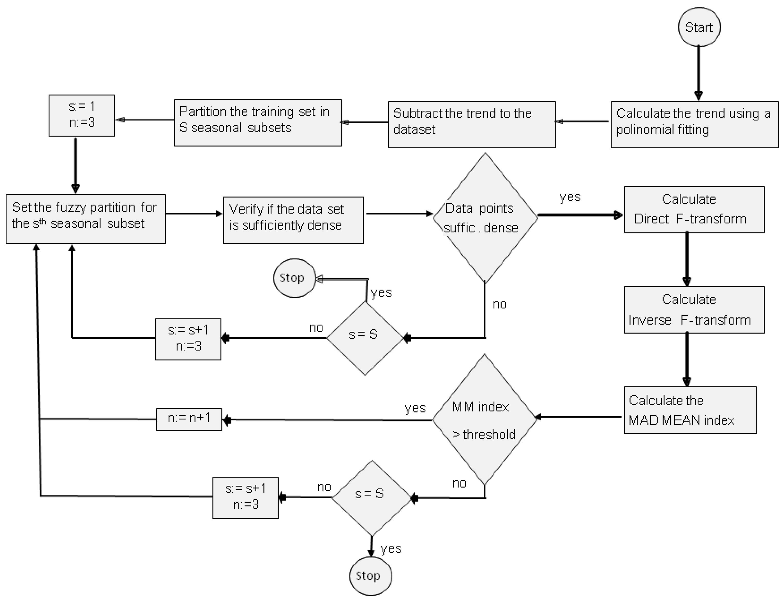
respectively. The inverse F-transform (13) approximates the seasonal fluctuation at the time t. In our method, we start with three basic functions and verify that the subset of data is sufficiently dense with respect to this fuzzy partition. After calculating the directed and inverse F-transform with Equations (12) and (13), respectively, we calculate the (MADMEAN)_s index for the sth fluctuation subset of data given as

$${(\mathrm{MADMEAN})}_s=\frac{{\displaystyle \sum _{j=1}^{M_s}\left|f_n^F(t_{}^{(j)})-y^{(j)}\right|}}{{\displaystyle \sum _{j=1}^{M_s}{y}^{(j)}}}$$

(14)

If Equation (14) is greater than an assigned threshold, than the process is iterated considering a fuzzy partition of dimension n:= n + 1; otherwise, the iteration process stops. Our algorithm is illustrated in Figure 3.

For the sth fluctuation subset, we obtain the inverse F-transform by using the following n(s) basic functions:

$$f_{n(s)}^F(t)={\displaystyle \sum _{h=1}^{n(s)}{F}_h\cdot A_h(t)}$$

(15)

For evaluating the value of the parameter y₀ at the time t in the sth seasonal period, we add to $f_{n(s)}^F(t)$ the trend calculated at the time t, i.e., trend(t), obtaining the following value:

$${\tilde{y}}_0(t)=f_{n(s)}^F(t)+trend(t)$$

(16)

For evaluating the accuracy of the results, we can use the MADMEAN index given by

$$\mathrm{MADMEAN}=\frac{{\displaystyle \sum _{j=1}^M\left|{\tilde{y}}_0(t^{(j)})-y_0^{(j)}\right|}}{{\displaystyle \sum _{j=1}^M{y}_0^{(j)}}}$$

(17)

For sake of completeness, we describe also the values of the above-cited indices:

-

Root Mean Square Error (RMSE) is defined as:

$$\mathrm{RMSE}={\left(\frac{{\displaystyle \sum _{j=1}^M{\left({\tilde{y}}_0(t^{(j)})-y_0^{(j)}\right)}^2}}{M}\right)}^{1/2}$$

(18)

-

Mean Absolute Percentage Error (MAPE) is defined as:

$$\mathrm{MAPE}=\left[\frac{1}{M}{\displaystyle \sum _{j=1}^M\left|\frac{{\tilde{y}}_0(t^{(j)})-y_0^{(j)}}{y_0^{(j)}}\right|}\right]\times 100$$

(19)

-

Mean Absolute Deviation (MAD) is defined as:

$$\mathrm{MAD}=\frac{{\displaystyle \sum _{j=1}^M\left|{\tilde{y}}_0(t^{(j)})-y_0^{(j)}\right|}}{M}$$

(20)

The TSSF algorithm is schematized in Appendix A. To evaluate the MADMEAN threshold, we consider a pre-processing phase in which we apply the k-cross-validation technique to control the presence of over-fitting in the learning data. We set a seasonal subset and we apply a random partition in k folds. The union of k − 1 subsets is used as training set and the other subset is used as validation set. Then we consider a fuzzy partition with n = 3 and apply Equation (17) to the training set calculating the MADMEAN index; then we apply Equation (18) to the validation test to calculate the RMSE index. We repeat this process for all the k folds, obtaining the mean MADMEAN and RMSE indexes as

$$\mathrm{MADMEAN}(n)=\frac{{\displaystyle \sum _{i=1}^k{\mathrm{MADMEAN}}_i(n)}}{k}$$

(21)

$$\mathrm{RMSE}(n)=\frac{{\displaystyle \sum _{i=1}^k{\mathrm{RMSE}}_i(n)}}{k}$$

(22)

where MADMEAN(n) and RMSE(n) are the mean MADMEAN and RMSE using the fuzzy partition size n, respectively.

We repeat this process using many values of n. Then, we plot in a graph the RMSE(n) by varying n. The threshold value is set as the mean MADMEAN obtained in correspondence of the value n for which there is a plateau in the RMSE graph.

In next section, we present the results of tests in which the TSSF algorithm is applied to seasonal time series. In our tests, we apply the pre-processing phase described below in which we partition the dataset in k folds, setting k = 10. Comparisons are pointed out with respect to ARIMA, the F-transform methods and SVM and ADANN proposed in [23].

5. Experiments on Time Series Data

In a first experiment, we use a dataset composed from climate data (mean, maximum and minimum temperature, pressure, speed of the wind, etc., measured every day) of Naples (Italy) collected at the webpage: www.ilmeteo.it/portale/archivio-meteo/Napoli. The following main climate parameters are measured every thirty minutes: Min temperature (°C), Mean temperature (°C), Max temperature (°C), Dew point (°C), Mean humidity (%), Mean view (km), Mean wind speed (km/h), Max wind speed (km/h), Gust of wind (km/h), Mean pressure on sea level (mb), Mean pressure (mb), and Millimeters of rain (mm).

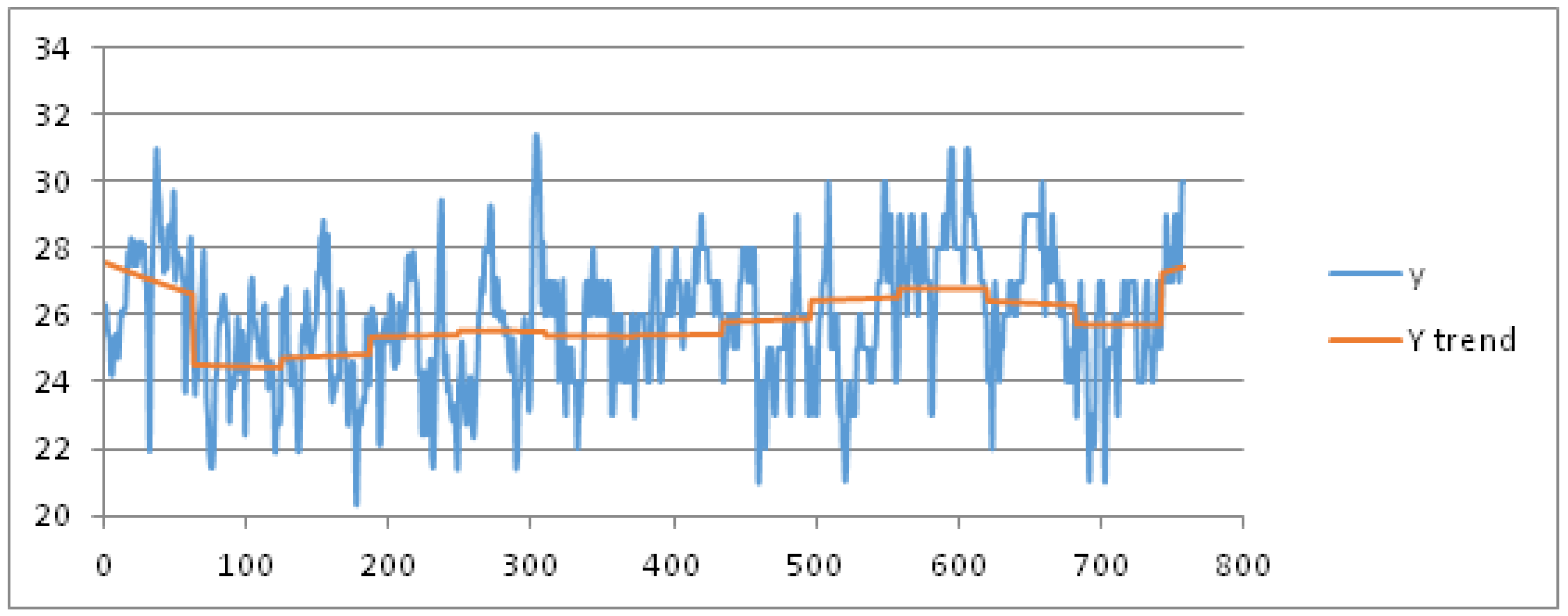
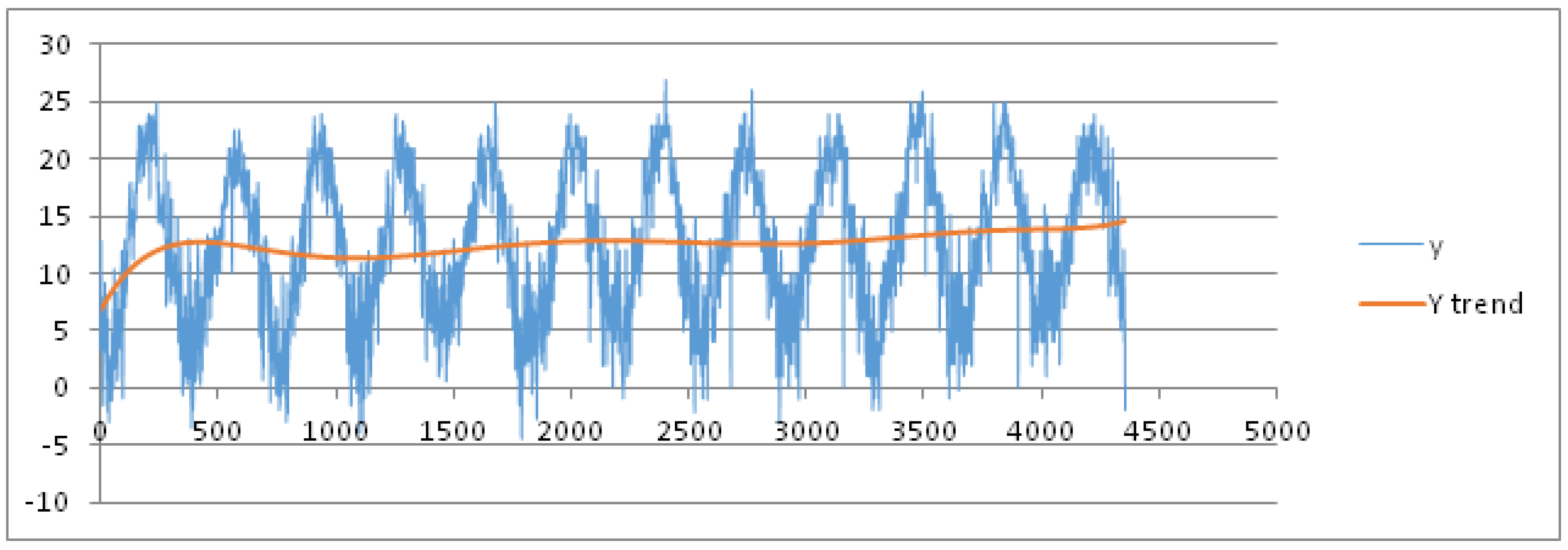
For sake of brevity, we limit the results for the parameters mean, max and min temperature. As training dataset, we consider these data recorded in the months July and August from 1 July 2003 to 16 August 2015, hence for 806 days represented as abscissas (via a number ID) in Figure 4 and Figure 5, respectively. The daily mean and max temperature is represented on the ordinate axis in Figure 4 and Figure 5, respectively. We obtain the best fit polynomial of nine degree ($y={\displaystyle \sum _{i=1}^9{a}_i}\cdot x^i$) (red color in Figure 4 and Figure 5) whose coefficients are given in Appendix B.

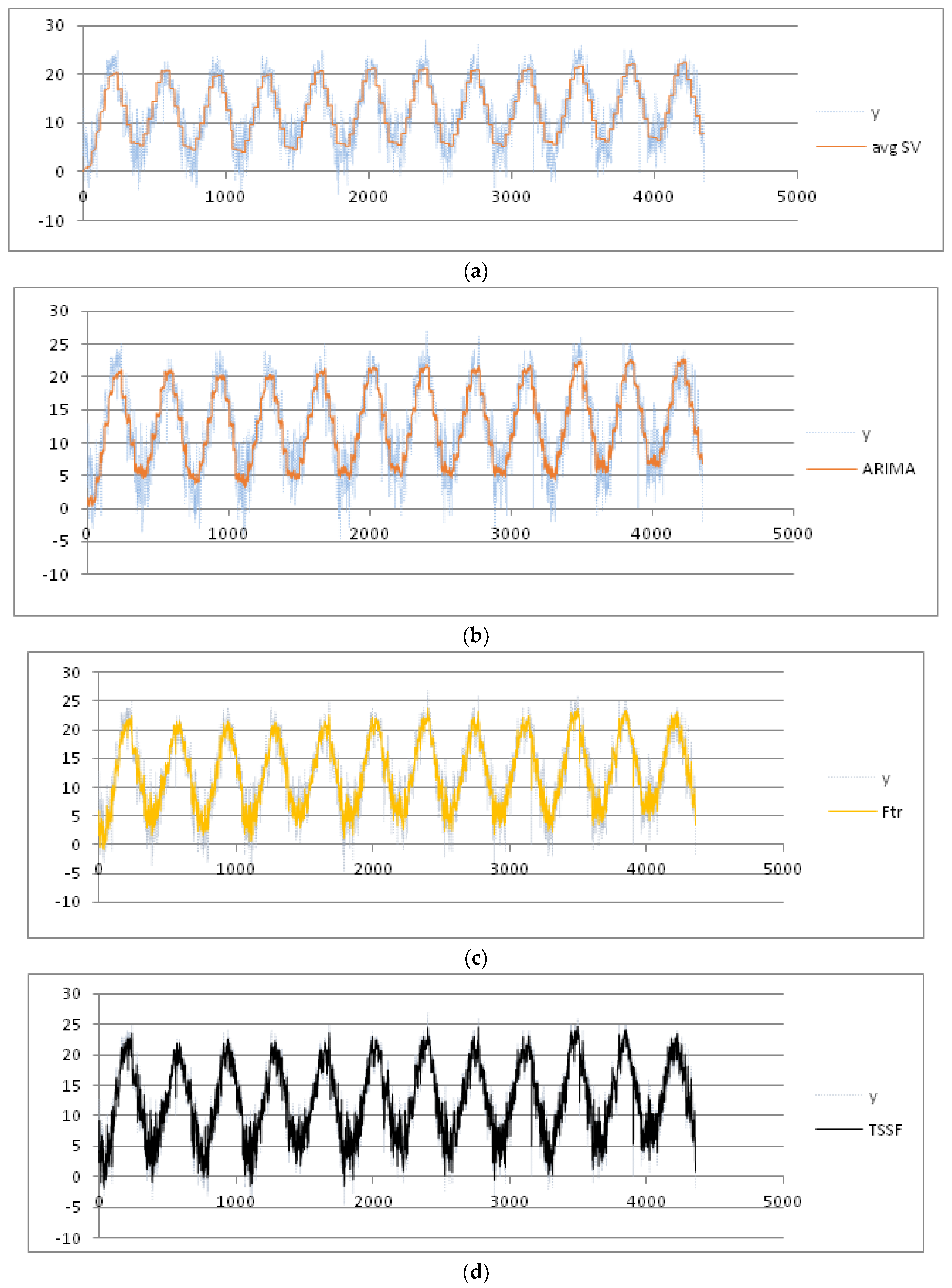
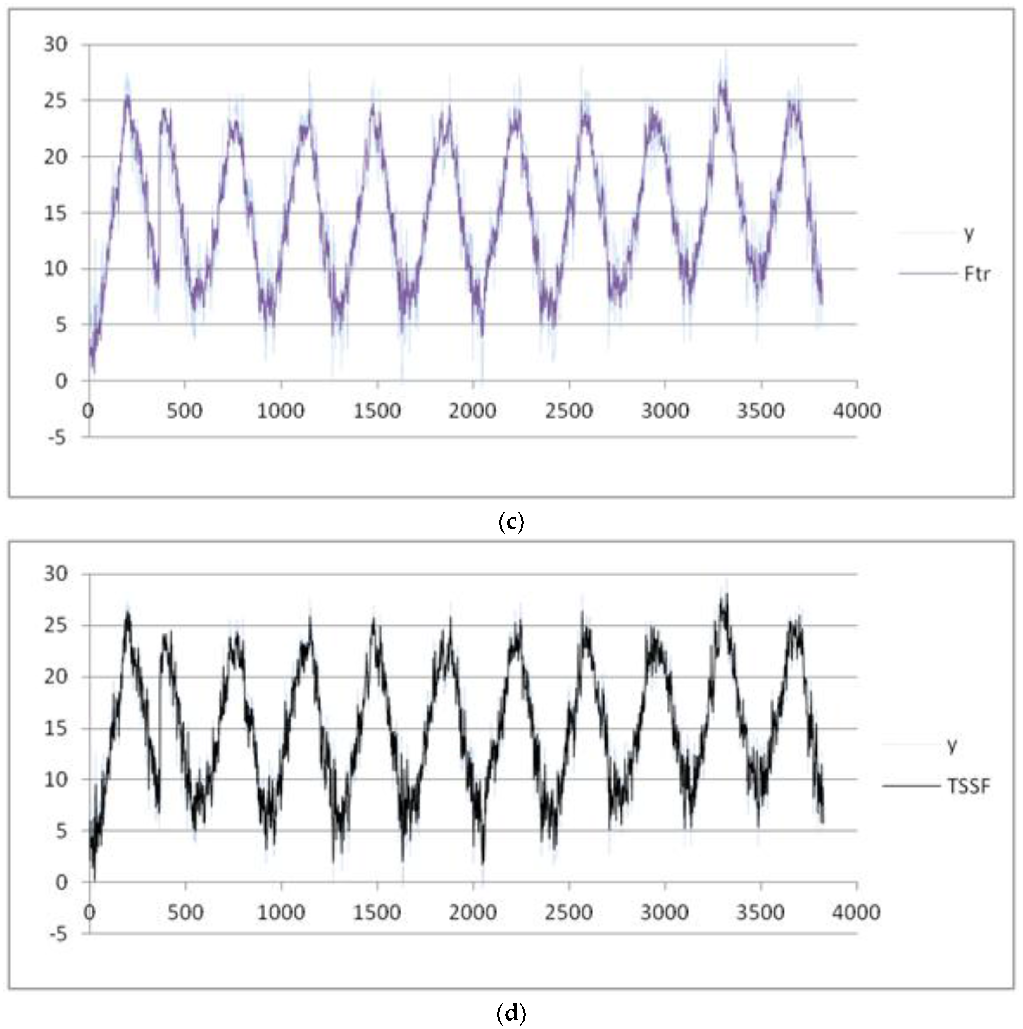
We consider the week as seasonal period, partitioning the data set into nine seasonal subsets: Week 27 (1 July) to Week 36 (31 August). After applying the pre-processing phase, we set the threshold of the MADMEAN index to the value 5. Then, we apply the TSSF algorithm to the daily mean and max temperature. We also give the results of the other three methods, plotted in Figure 6a–d and Figure 7a–d , respectively:

(1)

Average seasonal variation method [3] (labeled as avgSV): This method calculates the mean seasonal variation for each seasonal period and adds the mean seasonal variation to the trend value.

(2)

Seasonal ARIMA method: In our experiments, we used the forecasting tool ForecastPro [35]. As highlighted in [23], this tool is well known for ensuring the best performance in the use of forecasting ARIMA models.

(3)

F-transform prediction method [29]: This is applied to the complete dataset (labeled as F-transforms).

In

Table 1. RMSE, MAPE, MAD, and MADMEAN indices for the mean temperature.

Forecasting Method	RMSE	MAPE	MAD	MADMEAN
avgSV	1.78	5.60%	1.42	5.50
ARIMA	1.55	4.89%	1.24	4.80
F-transforms	1.61	4.96%	1.28	5.05
TSSF	1.37	4.29%	1.09	4.22

, we show the four indices obtained using the four methods. The best results for the mean temperature are obtained using the TSSF method, with a MADMEAN of 4.22.

In

Table 2. RMSE, MAPE, MAD and MADMEAN indices for the max temperature.

Forecasting Method	RMSE	MAPE	MAD	MADMEAN
avgSV	2.21	5.74%	1.74	5.70
ARIMA	1.93	5.03%	1.53	4.99
F-transforms	1.98	5.17%	1.56	5.13
TSSF	1.76	4.57%	1.39	4.53

, we show the four indexes obtained using the four methods. The best results for the max temperature are obtained using TSSF, with a MADMEAN of 4.53.

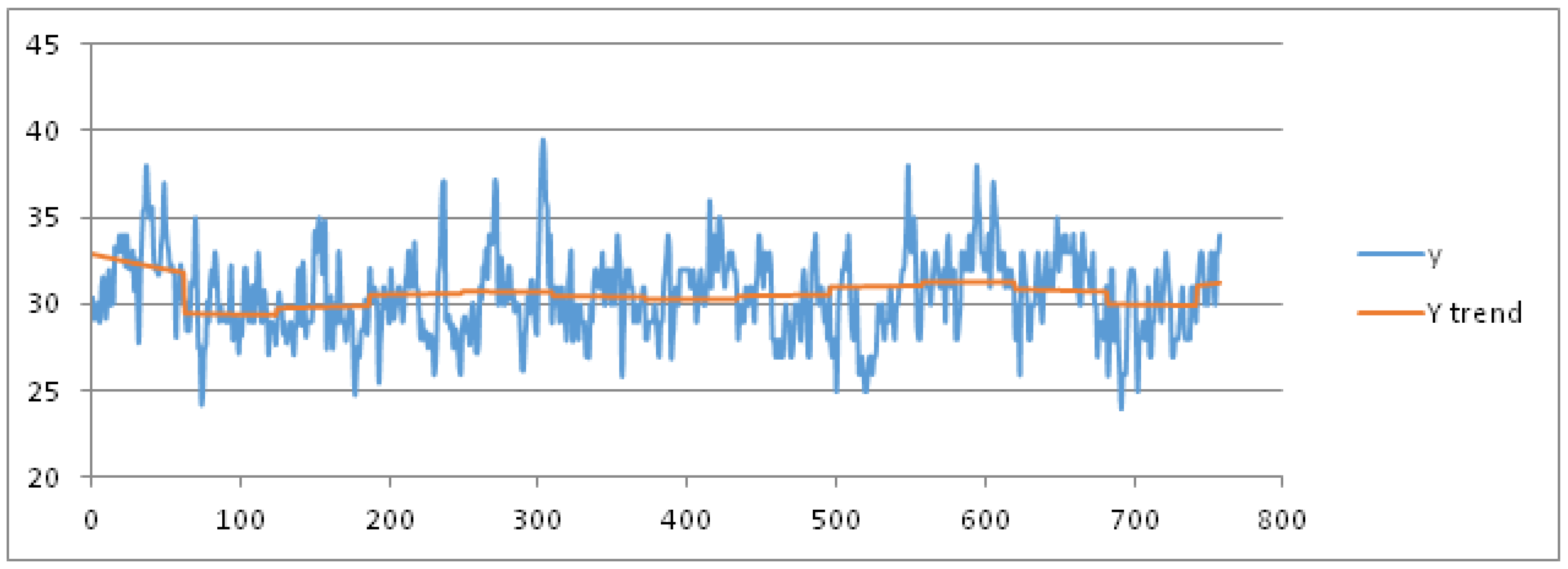
We now present the results of other experiments in which the variation of the min temperature is explored during the years. We assume the month as seasonal period: the training dataset is formed by all the measures recorded from 1 January 2003 to 31 December 2015. It is partitioned into 12 seasonal subsets corresponding to 12 months of a year. After applying the pre-processing phase, we set the threshold of the MADMEAN index to the value 6. In Figure 8, we show the data and the trend obtained using a best fit polynomial of nine degree (see Appendix A).

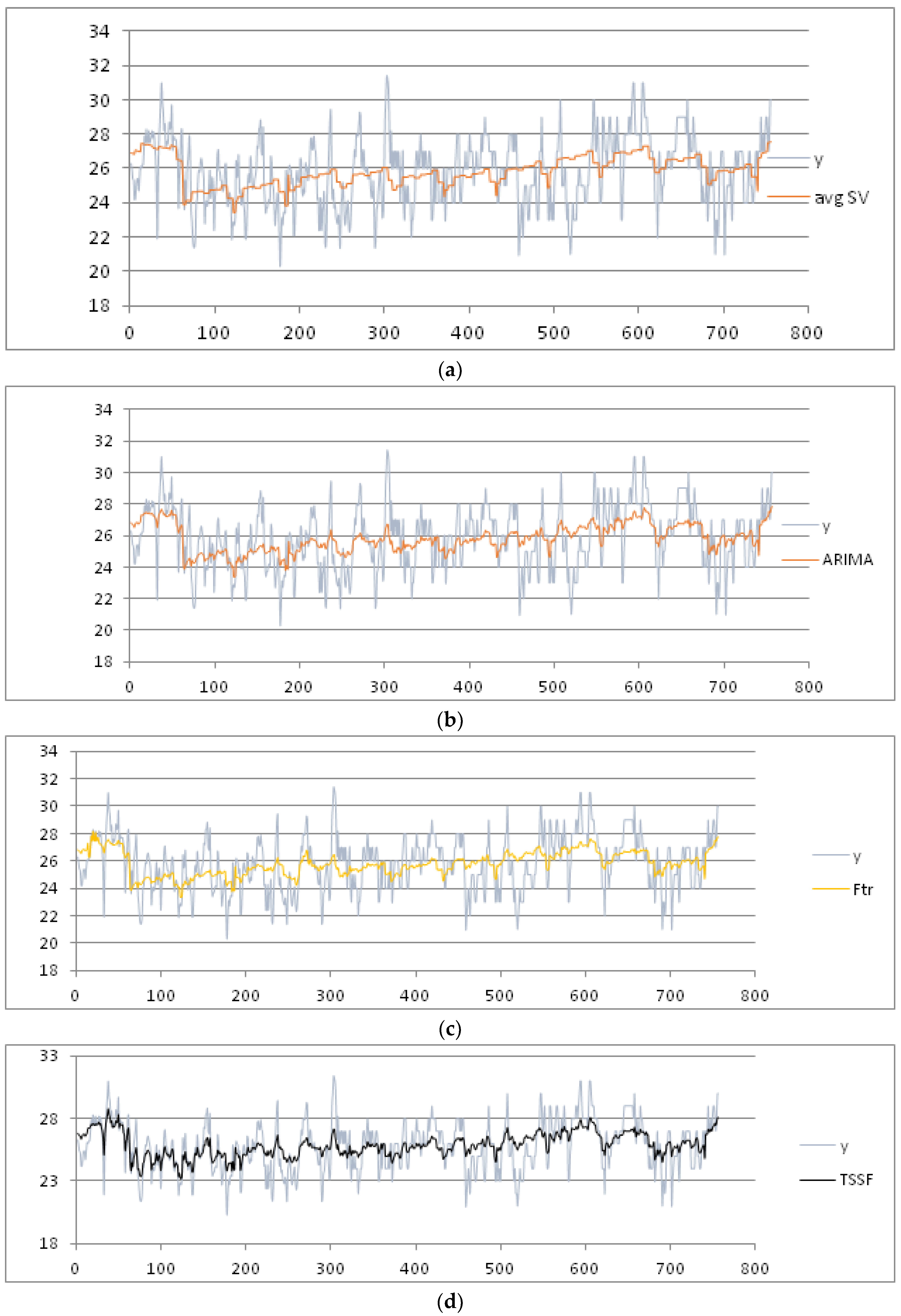
As we can observe in Figure 8, the seasonality of the data seems to be more evident than in the two previous examples. In Figure 9a–d, we plot the final results using the four forecasting methods.

In

Table 3. RMSE, MAPE, MAD and MADMEAN indices for the min temperature.

Forecasting Method	RMSE	MAPE	MAD	MADMEAN
avgSV	2.97	-	2.34	18.66
ARIMA	1.25		0.97	7.46
F-transforms	1.56	-	1.09	8.73
TSSF	0.87	-	0.66	5.26

, we show the indices obtained using the four methods. MAPE is not measurable because there are measures of min temperature equal to 0.00. The best results for the min temperature are obtained using the TSSF, with a MADMEAN of 5.26.

The results in Table 3 show that the TSSF is more efficient when the seasonality of the data is more pointed, such as the mean temperature time series. To test the reliability of the forecasting results obtained using the four forecasting methods, we have considered test datasets containing the measure of the analyzed parameter in a next time period and calculating the RMSE obtained with respect to the forecasted values. For the mean and max temperature parameters, we use a test dataset formed by the mean and max daily temperatures measured in the temporal interval 17 August 2015–31 August 2015. For the min temperature parameter, we use a test dataset formed by the min daily temperatures measured in the temporal interval 1 January 2015–31 August 2015. We apply the test datasets, measuring the RMSE obtained using the four methods. In addition, we also show the RMSE calculated by applying the SVM and ADANN algorithms proposed in [23], as shown in

Table 4. RMSE measured by using six different methods for the mean, max, min temperature.

Parameter	Training Dataset Dimension	Test Dataset Dimension	Seasonal Period	RMSE
				avgSV	ARIMA	F-transf.	TSSF	SVM	ADANN
Temp. mean	757	15	Week	1.83	1.58	1.62	1.39	0.88	0.87
Temp. max	757	15	Week	2.20	1.92	1.99	1.68	1.31	1.26
Temp. min	4354	212	Month	2.90	1.27	1.54	0.94	0.96	1.01

.

These results confirm that the performances obtained using the TSSF algorithm are better than the ones obtained using the avgSV, ARIMA and F-transform methods: the most reliable results are obtained for the third parameter, in which the seasonality is more regular. In addition, the performance obtained by applying SVM and ADANN algorithms to the first two time series improve those obtained by adopting the TSSF algorithm, but, in the third case, where the time series has best regularity, RMSE obtained using the TSSF, SVM and ADANN algorithms are indeed comparable.

We repeated these comparison tests by using other climatic datasets. For brevity, we show the results obtained by analyzing the trend of the daily mean temperature measured at the weather station Chiavari Caperana in the Italian Region Liguria; the data can be downloaded at the website (http://www.cartografiarl.regione.liguria.it/SiraQualMeteo/script/PubAccessoDatiMeteo.asp) of the webpage “Ambiente in Liguria”.

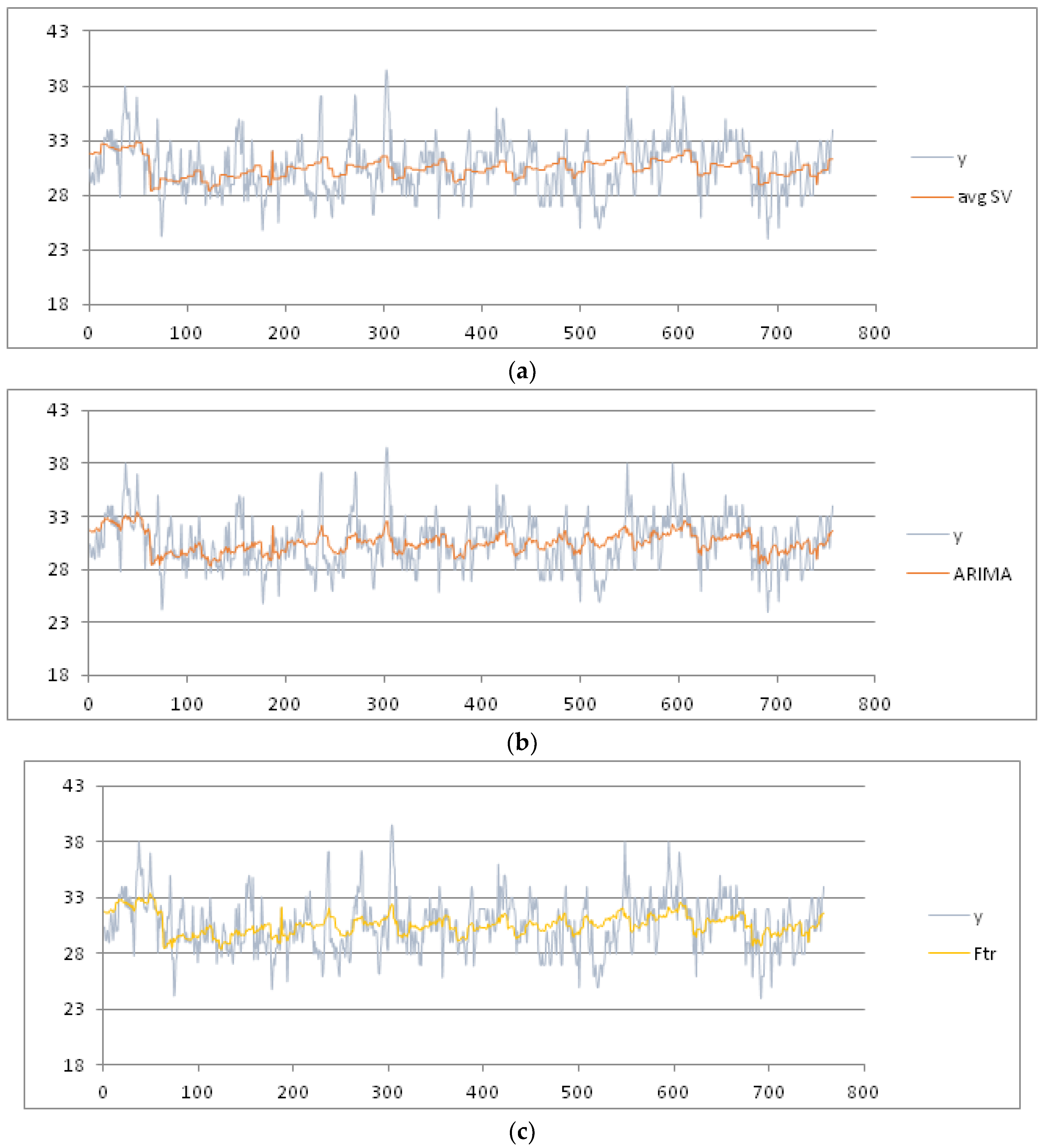
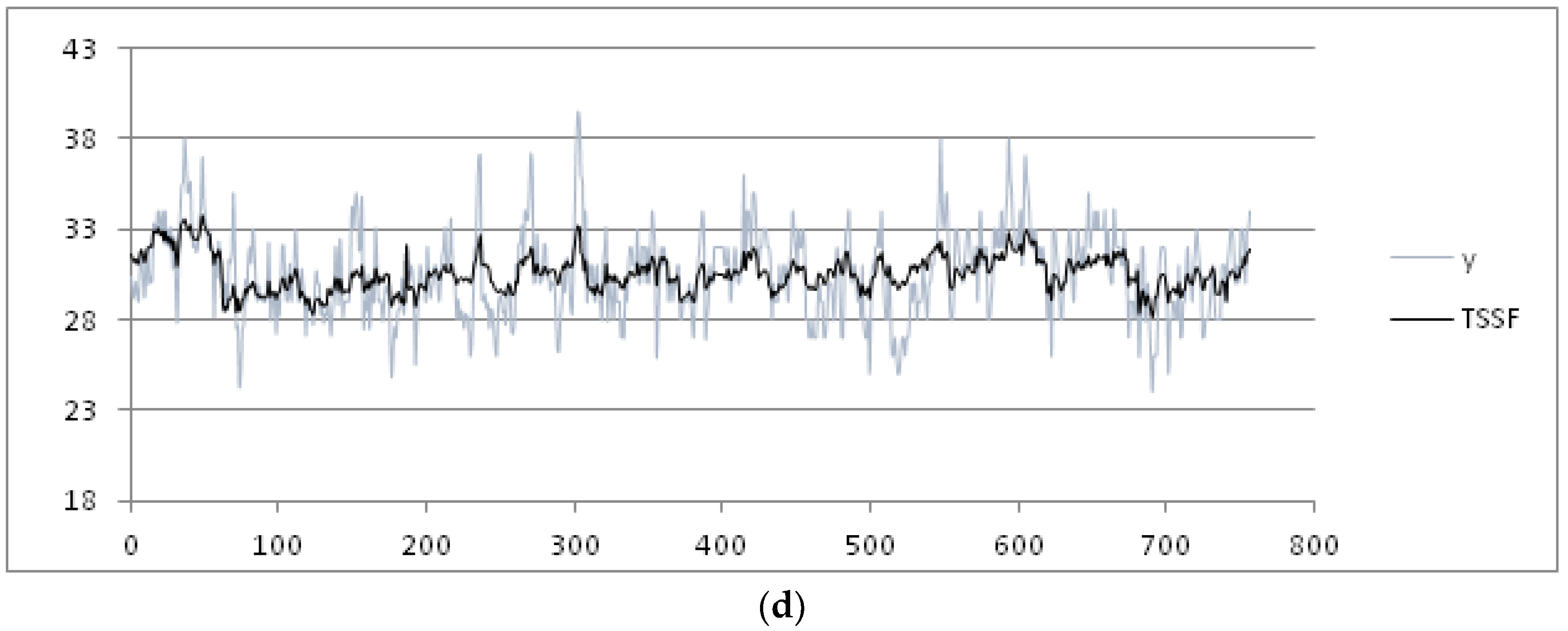
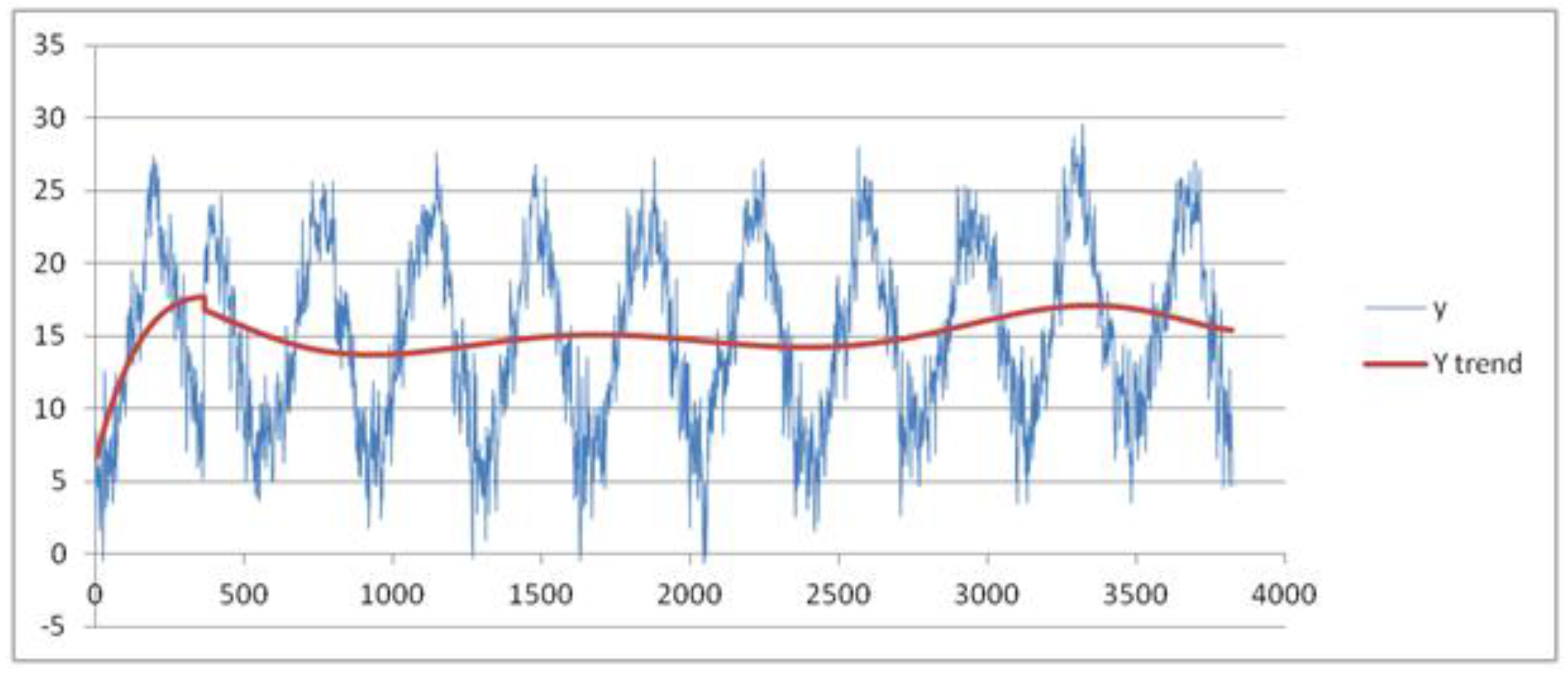
The analyzed data concern the measures (°C) of the daily mean temperature during the period 1 January 2006–31 December 2016. The month is considered as the seasonal period; the dataset is partitioned into 12 seasonal subsets corresponding to the 12 months of a year. After applying the pre-processing phase, we set the threshold of the MADMEAN index to the value 5.2.

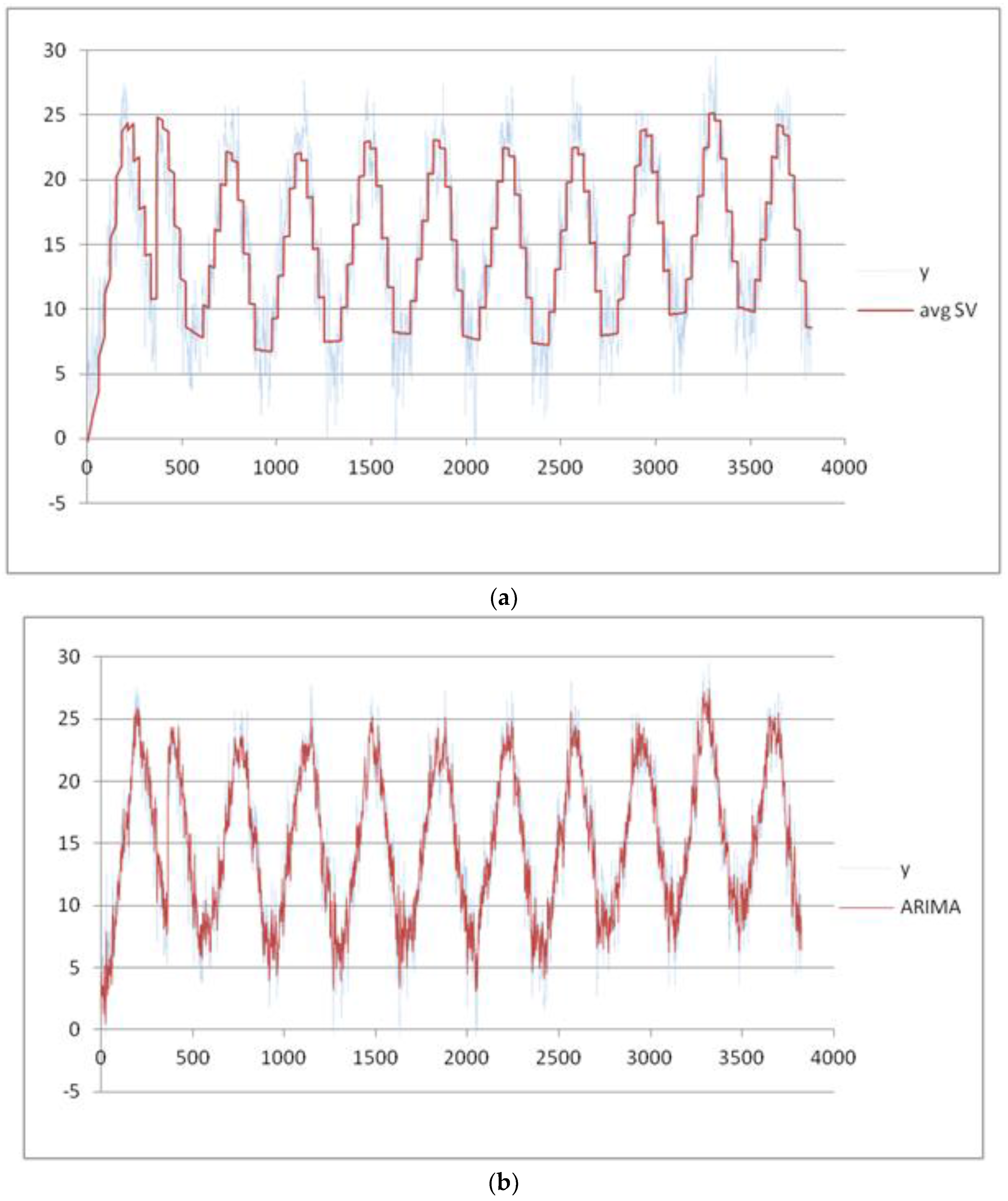
In Figure 10, we show the data and the trend obtained using a best fit polynomial of nine degree (see Appendix A and Appendix B). In Figure 11a–d, the results obtained using the four methods are plotted.

In

Table 5. RMSE, MAPE, MAD, MADMEAN indices for the mean temperature (Chiavari-Caperana weather station).

Forecasting Method	RMSE	MAPE	MAD	MADMEAN
avgSV	2.87	27.74%	2.14	16.19
ARIMA	1.13	12.37%	0.89	5.95
F-transforms	1.38	15.18%	1.10	7.30
TSSF	0.73	7.96%	0.58	3.83

, we show the four indexes obtained using the four methods. The best results for the mean temperature are obtained using TSSF, with a MADMEAN of 3.83.

The results in Table 5 confirm the ones obtained for the min temperature parameters in the weather dataset of Naples (Table 3): the TSSF gives better results than the ARIMA and F-transform algorithms, and is more efficient when the seasonality of the data is more regular. To test the reliability of the results obtained in Table 5, we have considered a test dataset containing the measure of the daily mean temperature during the period 1 January 2017–19 March 2017 and calculating the RMSE obtained with respect to the forecasted values. In

Table 6. RMSE in six methods for the mean temperature (Chiavari-Caperana weather station).

Parameter	Training Dataset Dimension	Test Dataset Dimension	Seasonal Period	RMSE
				avgSV	ARIMA	F-transf.	TSSF	SVM	ADANN
Temp. mean	3822	78	Month	2.85	1.15	1.40	0.85	0.88	0.87

, we show the RMSE measured in the ix methods for each parameter.

The results in Table 6 confirm that the performances obtained using the TSSF algorithm are better than the ones obtained using the avgSV, ARIMA and F-transform methods. Moreover, the performance of the TSSF algorithm is comparable with the ones obtained using the SVM and ADANN algorithms, as the time series shows a regular seasonality.

In

Table 7. RMSE in six methods for the mean temperature in various stations in Genova district (Italy).

Station	RMSE
	avgSV	ARIMA	F-transf.	TSSF	SVM	ADANN
Alpe Gorreto	2.98	1.20	1.49	0.84	0.81	0.83
Campo Ligure	2.74	1.09	1.34	0.76	0.71	0.76
Barbagelata	3.25	1.30	1.57	0.89	0.84	0.90
Camogli	3.39	1.38	1.68	0.95	0.88	0.86
Campo ligure	3.02	1.20	1.49	0.83	0.77	0.79
Carlasco	2.91	1.15	1.42	0.80	0.77	0.76
Chiavari	2.78	1.12	1.39	0.78	0.73	0.77
Genova Bolzaneto	2.95	1.16	1.41	0.81	0.77	0.75
Genova Pegli	3.34	1.29	1.64	0.94	0.89	0.88
Panesi	3.20	1.29	1.56	0.87	0.84	0.83
Rapallo	2.71	1.08	1.33	0.75	0.78	0.84
Rovegno	2.94	1.18	1.45	0.82	0.82	0.80
Tigliolo	3.06	1.24	1.52	0.85	0.80	0.85
Viganego	3.17	1.28	1.57	0.88	0.82	0.83

, we show the tests results obtained for the mean temperature using the seasonal datasets of the daily mean temperature measured by other stations in the district of Genova; the data were downloaded from the Liguria Region webpage “Ambiente in Liguria”. In each experiment, the season parameter is given by the month of the year.

Table 7 confirms the results of Table 6. The performances of the TSSF algorithm are better than the ones obtained using the avgSV, ARIMA and F-trasform methods and comparable with the ones obtained with the SVM and ADANN algorithms: the reason for this is that none of the time series in Table 7 has significant irregular variations.

6. Conclusions

We present a new method based on F-transforms for seasonal forecasting. The goal was to adapt the F-transform based forecasting method in [29] for the analysis of seasonal times series, improving its performances with respect to other known methods. Usually, ARIMA model has lower performance than models based on ANN and SVM, but these models are complex to manage: for instance, the choice of the input parameters often affects the reliability of the final results. Our results show that the TFSS method improves the performances of ARIMA, avgSV and F-transform forecasting methods. In addition, for time series in which the seasonality of the data is more regular, the performance obtained using the TFSS algorithm is comparable with the one obtained with SVM and ADANN models.

In future works, we shall try to improve TSSF for the management of time series that also contain irregular variations, comparing it with other soft computing algorithms.