Reconstructing Damaged Complex Networks Based on Neural Networks

Abstract

Despite recent progress in the study of complex systems, reconstruction of damaged networks due to random and targeted attack has not been addressed before. In this paper, we formulate the network reconstruction problem as an identification of network structure based on much reduced link information. Furthermore, a novel method based on multilayer perceptron neural network is proposed as a solution to the problem of network reconstruction. Based on simulation results, it was demonstrated that the proposed scheme achieves very high reconstruction accuracy in small-world network model and a robust performance in scale-free network model.

1. Introduction

Complex networks have received growing interest from various disciplines to model and study the network topology and interaction between nodes within a modeled network [1,2,3]. One of the important problems that are actively studied in the area of network science is the robustness of a network under random failure of nodes and intentional attack on the network. For example, it has been found that scale-free networks are more robust compared to random networks against random removal of nodes, but are more sensitive to targeted attacks [4,5,6]. Furthermore, many approaches have been proposed to optimize conventional networks against random failure and intentional attack compared to the conventional complex networks [7,8,9,10]. However, these approaches have been mainly concentrated on designing network topology based on various optimization techniques to minimize the damage to the network. So far, no work has been reported on techniques to repair and recover the network topology after the network has been damaged. Numerous solutions have been proposed on reconstruction of spreading networks based on spreading data [11,12,13], but the problem on the reconstruction of damaged networks due to random and targeted attacks has not been addressed before.

Artificial neural networks (NNs) have been applied to solve various problems in complex systems due to powerful generalization abilities of NNs [14]. Some of the applications where NNs have been successfully used are radar waveform recognition [15], image recognition [16,17], indoor localization [18,19], and peak-to-average power reduction [20,21]. In this paper, we propose a novel network reconstruction method based on the NN technique. To the best of our knowledge, this work is the first attempt to recover the network topology after the network has been damaged and also the first attempt to apply NN technique for complex network optimization. We formulate the network reconstruction problem as an identification of a network structure based on a much reduced amount of link information contained in the adjacency matrix of the damaged network. The problem is especially challenging due to (1) very large number of possible network configurations on the order of $2^{N^2}$, where N is the number of nodes and (2) very small number of node interaction information due to node removals. We simplify the problem by the following assumptions (1) average number of real connections of a network is much smaller than all the possible link configurations and (2) link information of M undamaged networks are available. Based on these assumptions, we chose the multiple-layer perceptron neural network (MLPNN), which is one of the frequently used NN techniques, as the basis of our method. We evaluate the performance of the proposed method based on simulations in two classical complex networks (1) small-world network and (2) scale-free networks, generated by Watts and Strogatz model and Barabási and Albert model, respectively.

The rest of the paper is organized as follows. Section 2 describes the small-world network model and scale-free network, followed by the network damage model. In Section 3, we propose the reconstruction method based on NN technique. In Section 4, we present the numerical results of the proposed method, and conclusions are given Section 5.

2. Model

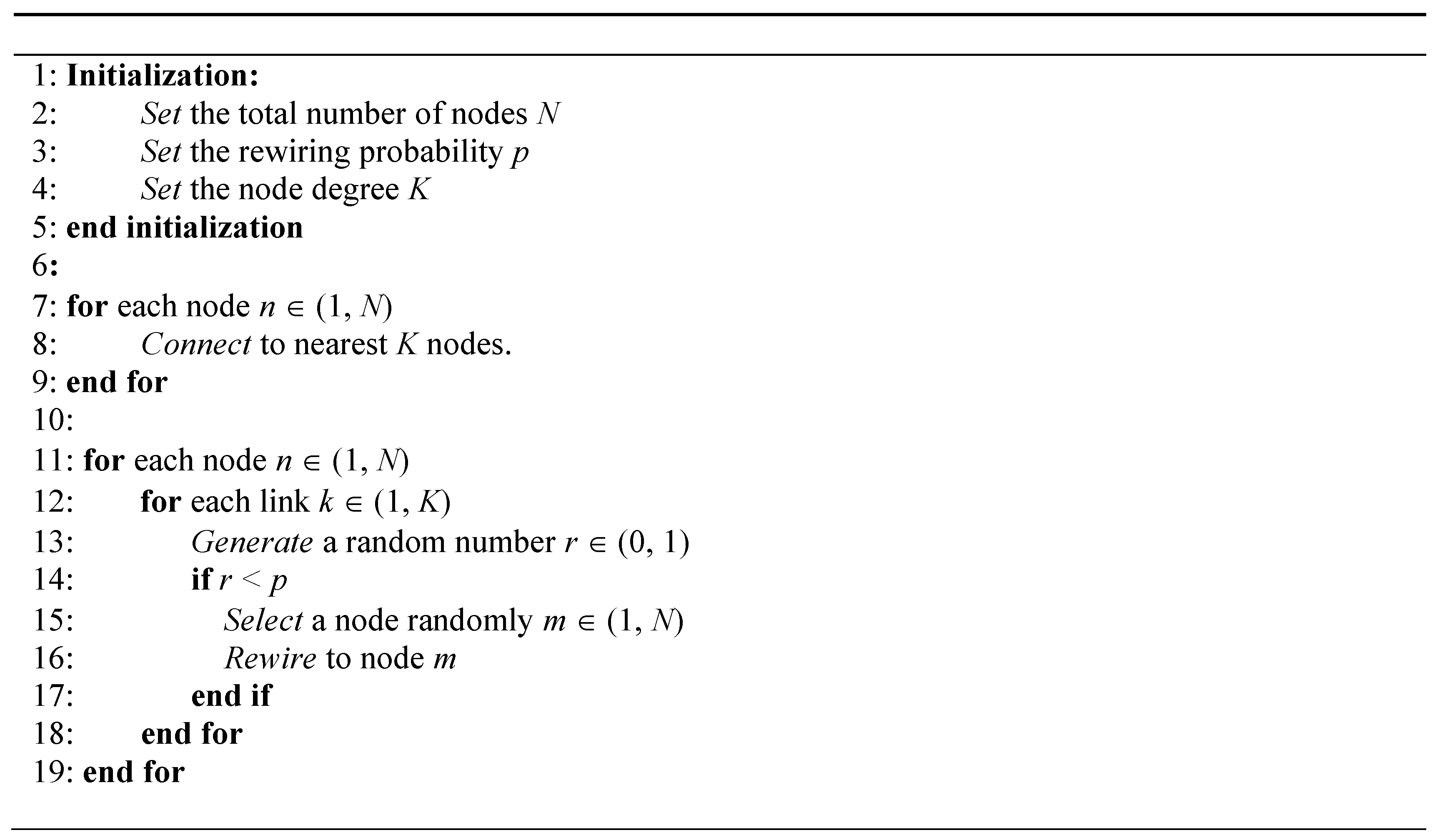
2.1. Small-World Network

Small-world network is an important network model with low average path length and high clustering coefficient [22,23,24]. Small-world networks have homogeneous network topology with a degree distribution approximated by the Poisson distribution. A small-world network is created based on a regular lattice such a ring of N nodes, where each node is connected to J nearest nodes. Next, the links are randomly rewired to one of N nodes in the network with probability p. The rewiring process is repeated for all the nodes n = 1 … N. By controlling the rewiring probability p, the network will interpolate between a regular lattice (p = 0) to a random network (p = 1). Figure 1 shows the detailed algorithm for small-world network construction in pseudocode format.

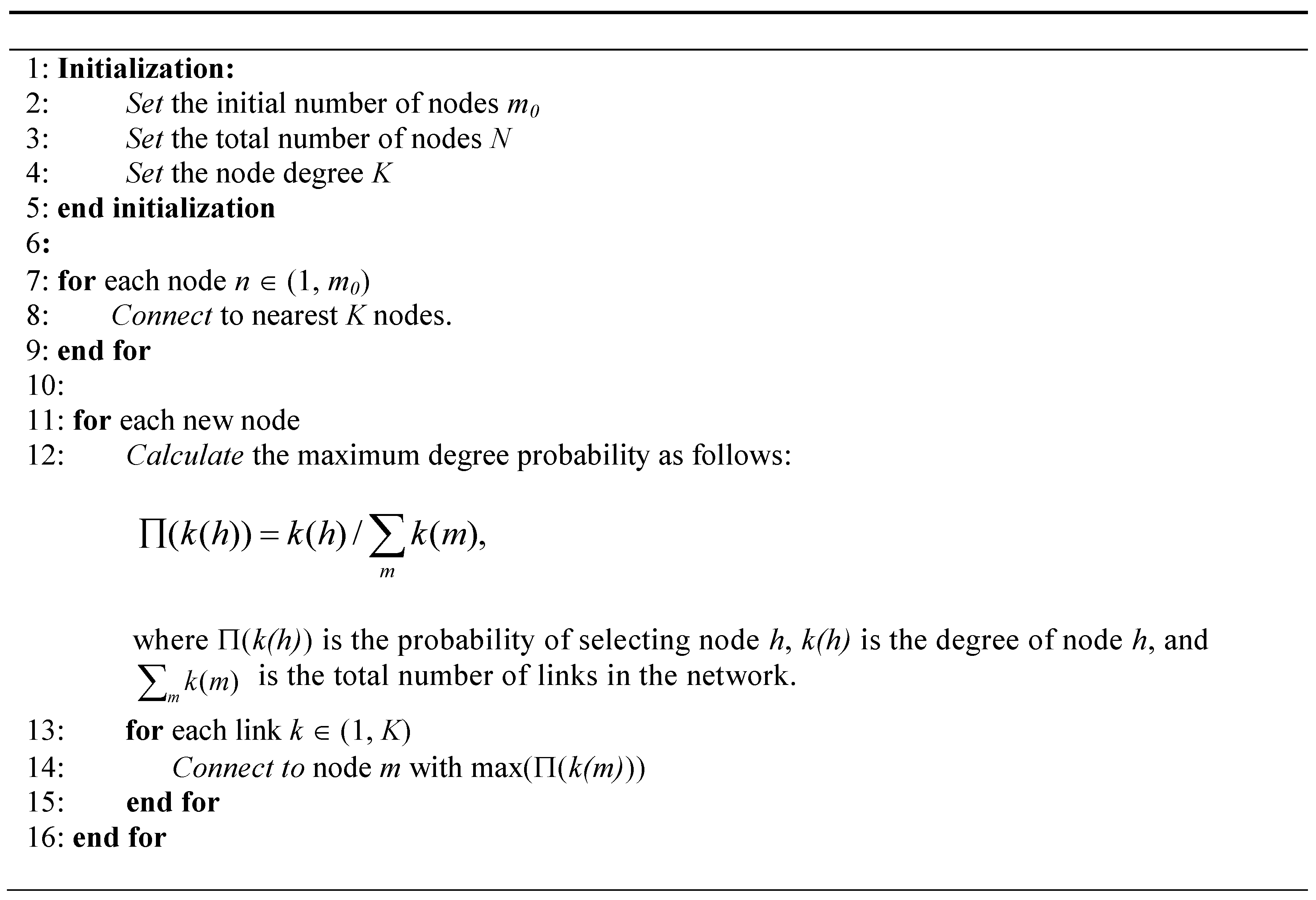
2.2. Scale-Free Network

Scale-free networks, such as Barabási and Albert (BA) network, are evolving networks that have degree distribution following power-law model [4,5,6]. Scale-free networks consist of a small number of nodes with very high degree of connections and rest of the nodes with low degree connections. A scale-free network starts the evolution process with a small number of m₀ nodes. Next, a new node is introduced to the network and attaches to m existing nodes with high degree k. The process consisting of new node introduction and preferential attachment is repeated until a network with N = t + m₀ nodes has been constructed. Figure 2 shows the detailed algorithm for scale-free network construction in pseudocode format.

2.3. Network Damage Model

We simulate the damage process on complex networks by considering the random attack model. In the random attack model, nodes are randomly selected and removed. Note that when a node is removed, all the links connected to that node are also removed [25]. To evaluate the performance of the proposed reconstruction method, the difference in the number of links between the original network and the reconstructed network is used and represented as probability of reconstruction error, P_RE, that is defined as follows:

$$P_{RE}=\frac{N_{L,diff}}{N_L}\hspace{0.17em},$$

(1)

where N_L is the total number of existing links in the complex network that were damaged due to random attack and N_L,diff is the total number of links in the reconstructed network that are different from the links in the original network before any node removal. For example, let us assume that the number of nodes N = 4 and the node pair set in the original network is equal to E_o = {(1, 2), (1, 4), (2, 3), (3, 4)}. If the reconstructed network has node pair set as E_r = {(1, 2), (1, 3), (1, 4), (2, 3)}, then N_L,diff = 2 and N_L = 4, giving us P_RE = 0.5. Note that the estimated links in the reconstructed network that were not in the original network, in additions to links that were not reproduced, are all counted as errors.

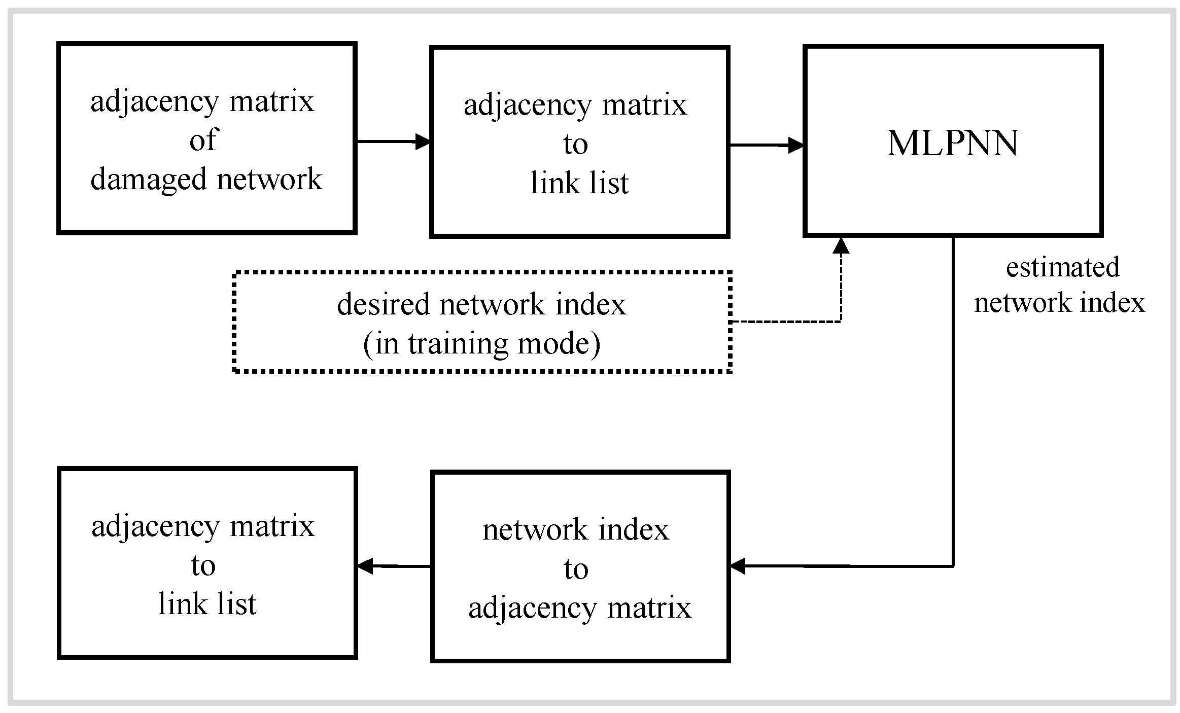
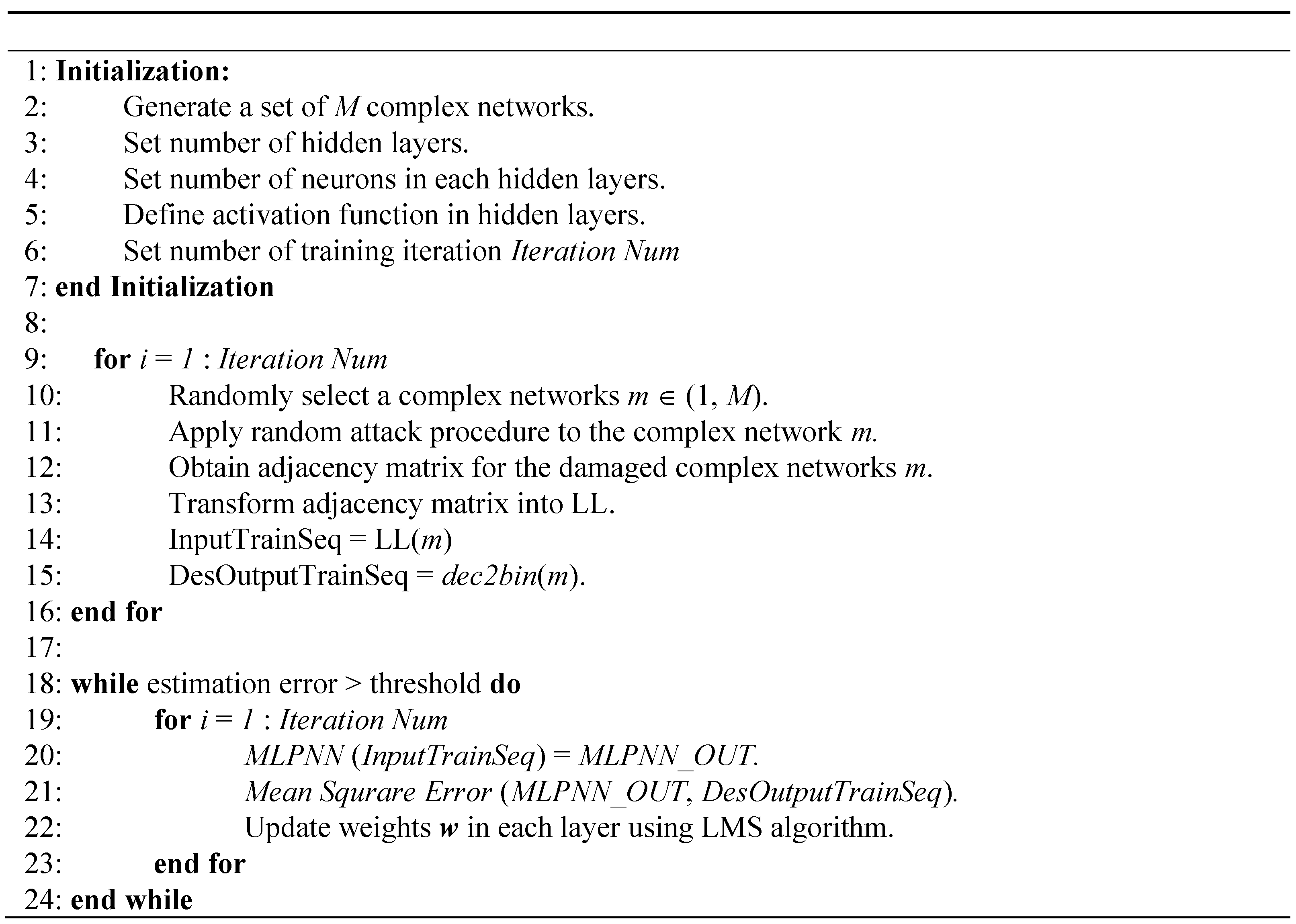
3. Reconstruction Method

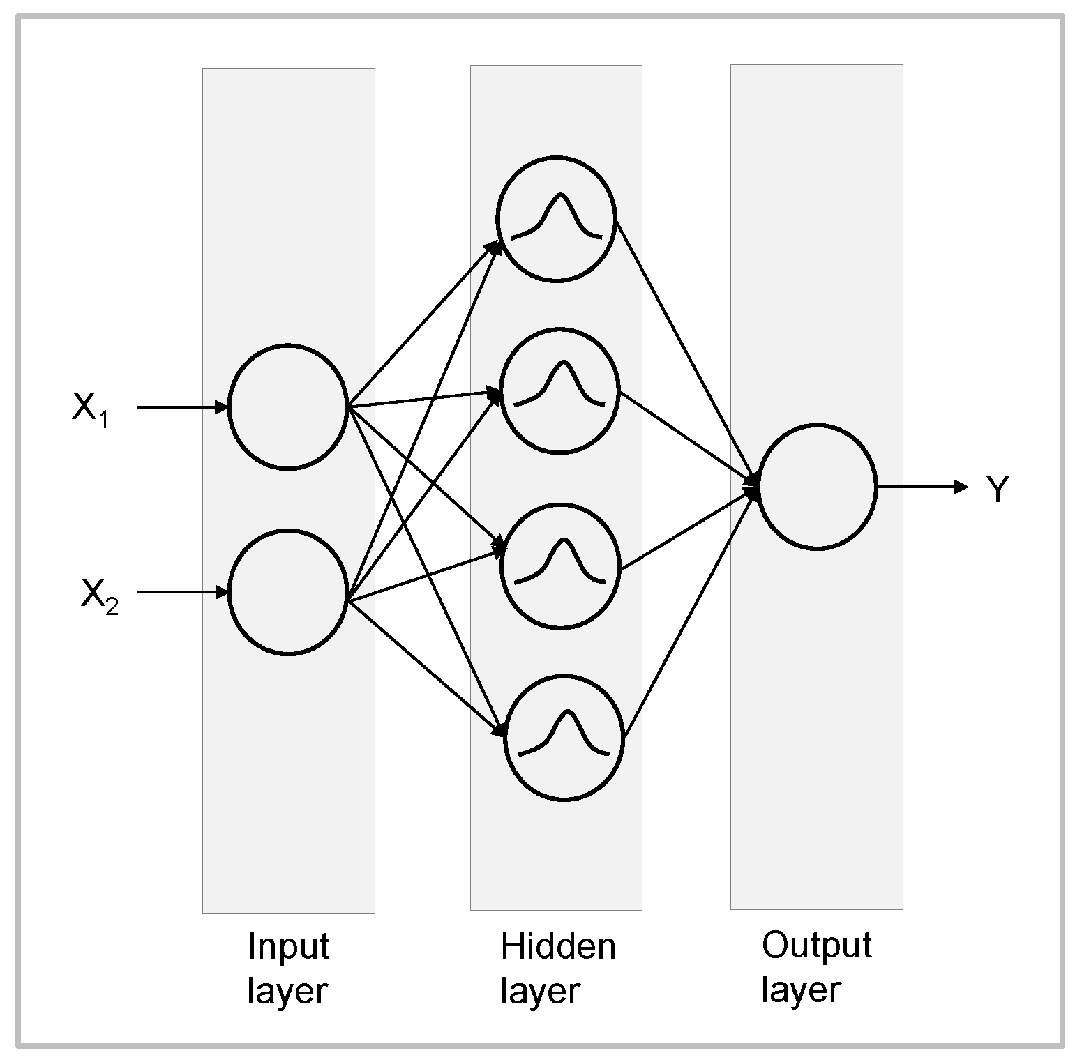
3.1. Neural Network Model

Neural networks are important tools that are used for system modeling with good generalization properties. We propose to use MLPNN employing backpropagation based supervised learning in this work. A MLPNN has three types of layers: An input layer, an output layer, and multiple hidden layers in between the input and output layer as shown in Figure 3. The input layer receives input data and is passed to the neurons or units in the hidden layer. The hidden layer units are nonlinear activation function of the weighted sum of inputs from the previous layer. The output of the jth unit in the hidden layer O(j) can be represented as [26]

$$A(j)={\displaystyle \sum _{i=1}^{m}w(j,i)}\hspace{0.17em}O(i)\hspace{0.17em}-U(j),$$

(2)

$$O(j)=\Im (A(j))\hspace{0.17em}=\frac{1}{1+e^{-A(j)}},$$

(3)

where A(j) is the activation input to jth hidden layer unit, w(i, j) is the weights from unit i to j, O(j) is the input to unit j, U(j) is the threshold of unit j, and ℑ (•) is a nonlinear activation function such as sigmoid function, as shown in Equation (3), hardlimit function, radial basis function, and triangular function. The number of units in the output layer is equal to the dimension of the desired output data format. The weights on the network connections are adjusted using training input data and desired output data until the mean square error (MSE) between them are minimized. To implement the MPLNN, the feedforwardnet function provided by the MATLAB Neural Network Toolbox was utilized. Additionally, the MPLNN weights were trained using the Levenberg-Marguardt algorithm [27].

3.2. Neural Network Based Method

To reconstruct the network topology of a damaged complex network due to random attack, we apply MLPNN as a solution to solve the complex network reconstruction problem. One of the key design issues in MLPNN is the training process of weights on the network connections such that the MLPNN is successfully configured to reconstruct damaged networks. Usually, a complex network topology is represented by an adjacency matrix describing interactions of all the nodes in the network. However, an adjacency matrix is inappropriate as training input data for MLPNN training process due to its complexity. Thus, we define a link list (LL) that contains binary elements representing existence of node pairs among all possible combination of node pairs $\left(\begin{array}{l}N\\ 2\end{array}\right)$, where N is the number of nodes in the network. For example, for a network with N = 4, possible node pair set is equal to, E = {(1, 2), (1, 3), (1, 4), (2, 3), (2, 4), (3, 4)}. If a network to be reconstructed has four nodes and four links given by E = {(1, 2), (1, 4), (2, 3), (3, 4)}, then LL = [1 0 1 1 0 1], where 1 s represents the existence of the four specific links among six possible ones. To obtain the training input data, M networks are damaged by randomly removing f percent of N nodes in a network. As shown in Figure 4, the proposed method consists of the following modules: Adjacency matrix of damaged network input module, adjacency matrix to link list transformation module, MLPNN module, and network index to adjacency matrix transformation module. In the second module, the adjacency matrices of the damaged networks are pre-processed into LLs that can be entered into the MLPNN. Note that the input dimension of the MLPNN is equal to the dimension of the training input data format. Thus, input dimension of the MLPNN is equal to $\left(\begin{array}{l}N\\ 2\end{array}\right)$. As for the desired output data, which is the output of the MLPNN module, binary sequence numbers are used to represent the indices of the original complex networks that have been damaged. The number of MLPNN output will depend on the number of training networks used to train the MLPNN. For example, eight binary outputs will be sufficient to represent 256 complex networks. Based on the training input data and desired output data, representing network topology of different complex networks, the goal of the MLPNN is to be able to identify, reconstruct, and produce node pair information of the original network, among numerous networks used to train the neural network. The detailed training algorithm of MLPNN is described in Figure 5.

4. Performance Evaluations

4.1. Simulation Environment

We study and evaluate the proposed reconstruction method based on the probability of reconstruction error P_RE described in Section 2. For the network damage model, we assume random attack process, where nodes are randomly removed with attached links. The MLPNN used in our method has two hidden layers with 64 neurons in the first layer and four neurons in the second layer. The nonlinear activation function in the hidden layer is chosen to be triangular activation function. The number of inputs to the MLPNN depends on the number of nodes in the network. To train and test the MLPNN, using complex networks with N = 10, N = 30, and N = 50, the number of inputs are set equal to the possible number of node pair combinations, which are 45, 435, and 1225, respectively. As for the number of outputs, eight are chosen to represent maximum number of 256 complex networks. The training input and output data patterns are randomly chosen from LL of M damaged complex networks with different percentage f of failed nodes out of total N nodes and corresponding indices of the complex networks.

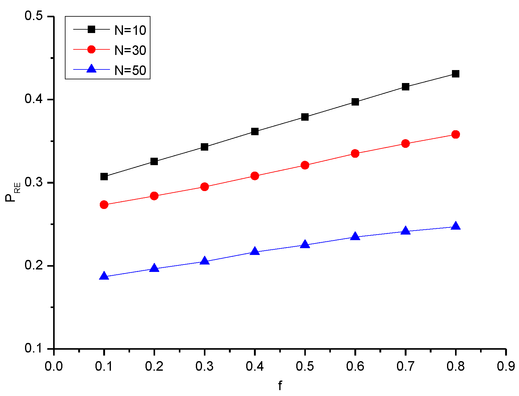
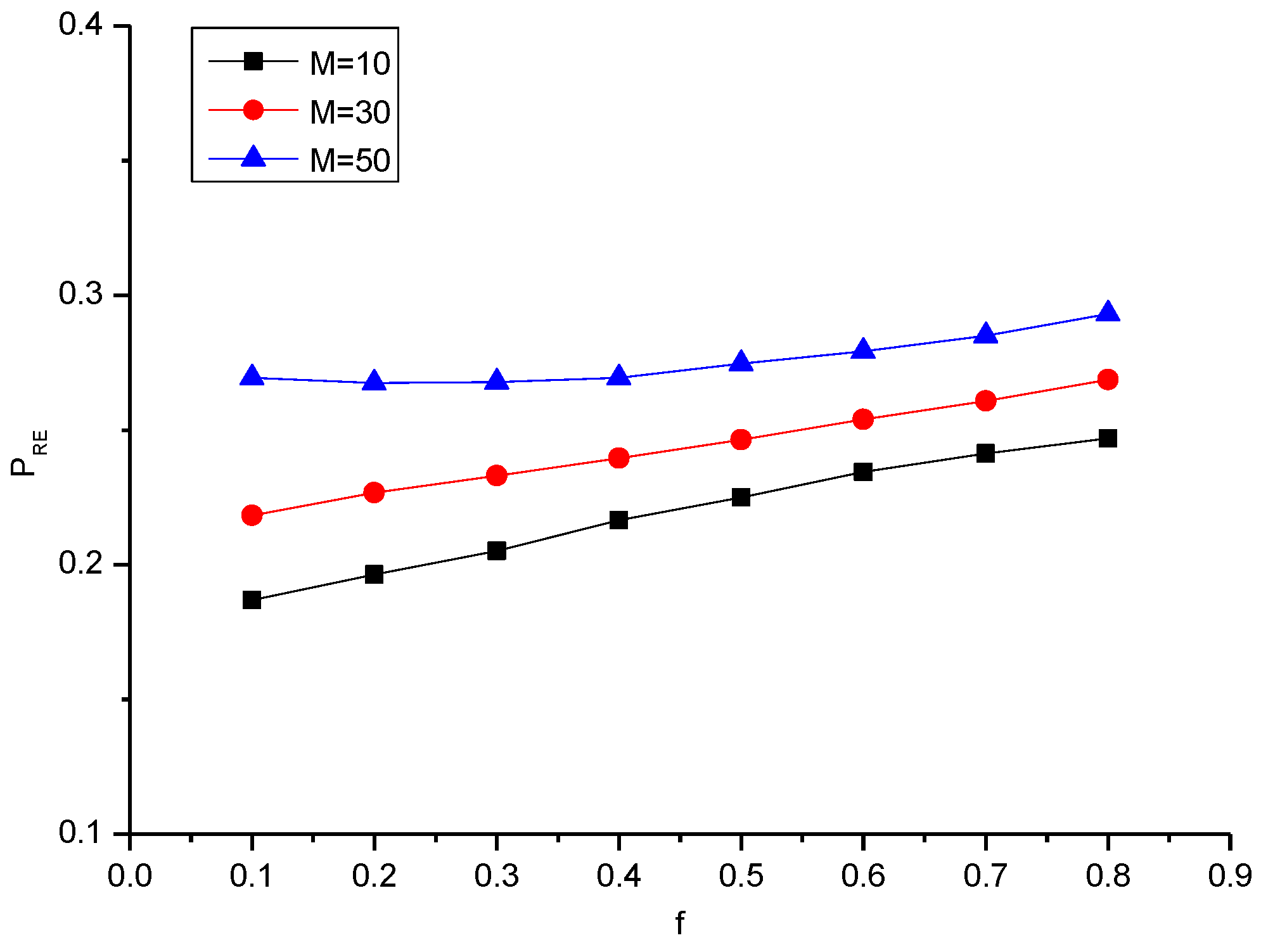
4.2. Small-World Network

To evaluate the performance of the proposed method in small-world network model, the network is implemented based on the algorithm described in Figure 1. Figure 6 and

Table 1. Probability of reconstruction error for small-world networks with N = 10, N = 30, N = 50, M = 10, and p = 0.15.

N/f	0.1	0.2	0.3	0.4	0.5	0.6	0.7	0.8
10	0.307	0.325	0.343	0.361	0.379	0.397	0.415	0.431
30	0.273	0.284	0.295	0.308	0.321	0.335	0.347	0.358
50	0.186	0.196	0.205	0.216	0.225	0.234	0.241	0.246

shows the reconstruction error probability as a function of percentage of random node failure f. Furthermore, we study the influence of the number of node on the network reconstruction performance with N = 10, N = 30, and N = 50. The initial degree K of the network is set to two and the links are randomly rewired with probability p = 0.15. One can see that with the increase in the number of node failures, the reconstruction performance deteriorates for all different N, but for f = 0.1, P_RE is less than 0.35 and for f = 0.5, P_RE is less than 0.5. In another words, the proposed method can reconstruct almost close to 70% of the network topology for 10% node failures and more than 60% of the network topology for 50% node failures. Note that lower reconstruction error probability is observed for larger number of nodes. The reason for this results is due to the higher dimension of input data to the MLPNN, e.g., 1225 for N = 50. Furthermore, from the figure, we observe that P_RE is less than what one might expect for the case where most of the nodes are destroyed, e.g., f = 0.7. This phenomenon is due to the large number of overlap in the node connections in LL among the M damaged networks due to small rewiring probability p. To study how the rewiring probability affects the reconstruction accuracy, simulations are performed with p = 0.3, p = 0.5, and p = 0.7, as shown in Figure 7 and

Table 2. Probability of reconstruction error for small-world networks with p = 0.3, p = 0.5, p = 0.7, M = 10, and N = 50.

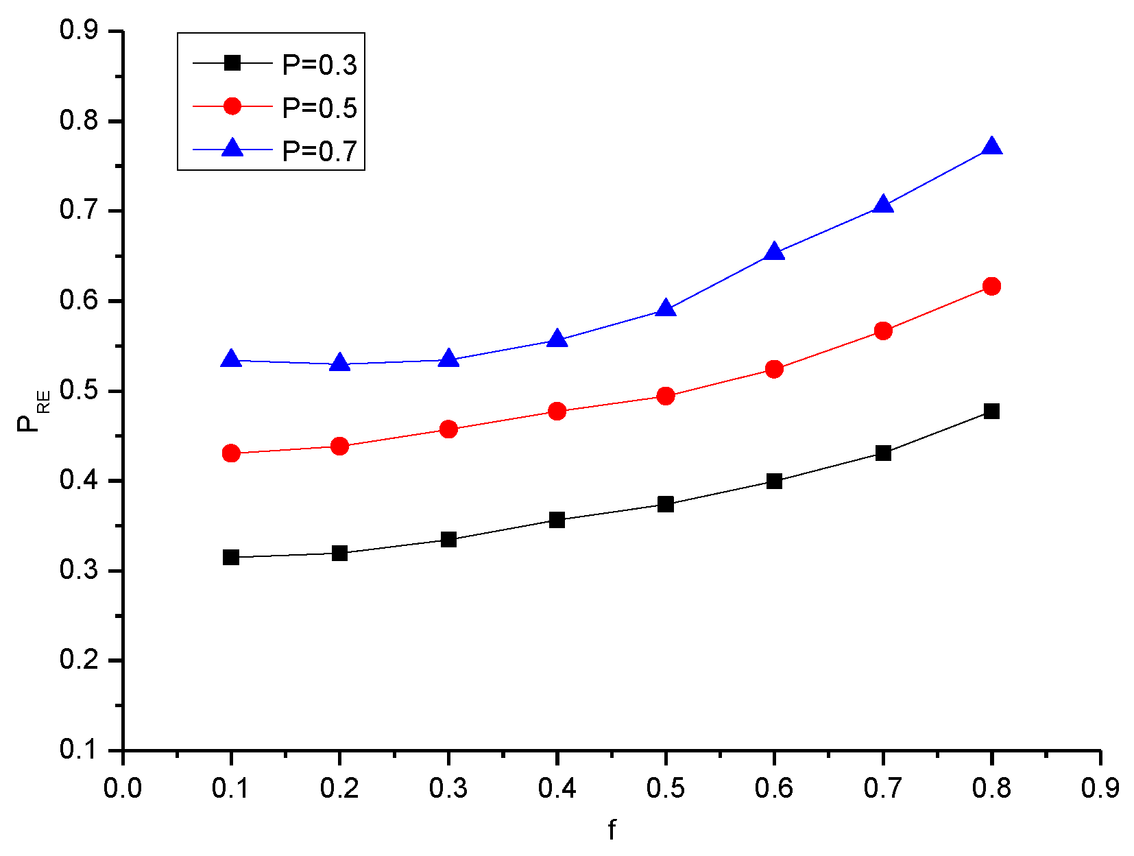
P/f	0.1	0.2	0.3	0.4	0.5	0.6	0.7	0.8
0.3	0.315	0.319	0.334	0.356	0.373	0.399	0.431	0.477
0.5	0.430	0.438	0.457	0.477	0.494	0.524	0.566	0.616
0.7	0.534	0.529	0.534	0.556	0.590	0.653	0.705	0.770

. From the figure, we can see that there is a significant deterioration in performance in reconstruction accuracy with increase in rewiring probability p. This is because the small-world network topology becomes increasingly disordered with increase in rewiring probability and results in decrease in ability of the proposed method to reproduce the original network topology.

However, even in the case of high rewiring probability p = 0.5, 50% of links can be successfully estimated. In Figure 8 and

Table 3. Probability of reconstruction error for small-world networks with M = 10, M = 30, M = 50, N = 50, and p = 0.15.

M/f	0.1	0.2	0.3	0.4	0.5	0.6	0.7	0.8
10	0.186	0.196	0.205	0.216	0.225	0.234	0.241	0.246
30	0.218	0.226	0.233	0.239	0.246	0.253	0.260	0.268
50	0.26	0.267	0.267	0.269	0.274	0.279	0.285	0.293

, we study the influence of the number of networks M that were used to train and test the MLPNN on the reconstruction performance. The number of nodes N is assumed to be 50 and the rewiring probability p is set to 0.5. It can be observed from the figure that there is a small degradation in performance with increase in M, but, P_RE remains less than 0.3.

4.3. Scale-Free Network

The proposed method is also evaluated in scale-free network model that is generated using the algorithm described in Figure 2. Figure 9 and

Table 4. Probability of reconstruction error for scale-free networks with N = 10, N = 30, N = 50, M = 10, and m₀ = 2.

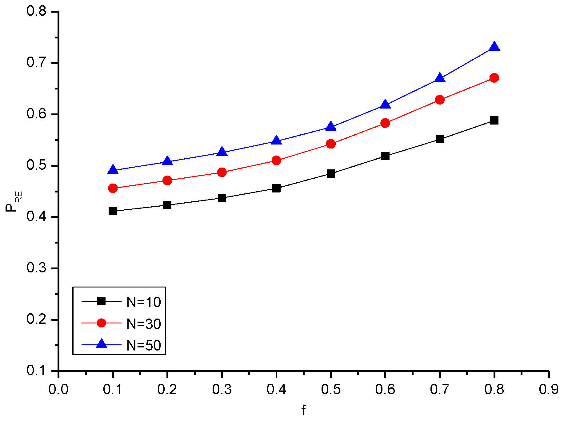
N/f	0.1	0.2	0.3	0.4	0.5	0.6	0.7	0.8
10	0.411	0.423	0.437	0.455	0.484	0.518	0.551	0.588
30	0.455	0.471	0.487	0.510	0.542	0.582	0.628	0.671
50	0.490	0.507	0.525	0.547	0.575	0.618	0.669	0.730

compares the reconstruction error probability for different number of nodes N = 10, N = 30, and N = 50. The initial number of nodes m₀ was set to two and the node degree K = 2 for the preferential attachment process. Figure 9 shows that the reconstruction accuracy in scale-free network model is significantly lower compared to the small-world network. The reason for the poor performance is that the network topologies of M scale-free networks are more complex compared to the small-world network models. Furthermore, the links in LL between the M damaged networks do not overlap as much as in the small-world network models. In Figure 10 and

Table 5. Probability of reconstruction error for scale-free networks with M = 10, M = 30, M = 50, N = 30, and m₀ = 2.

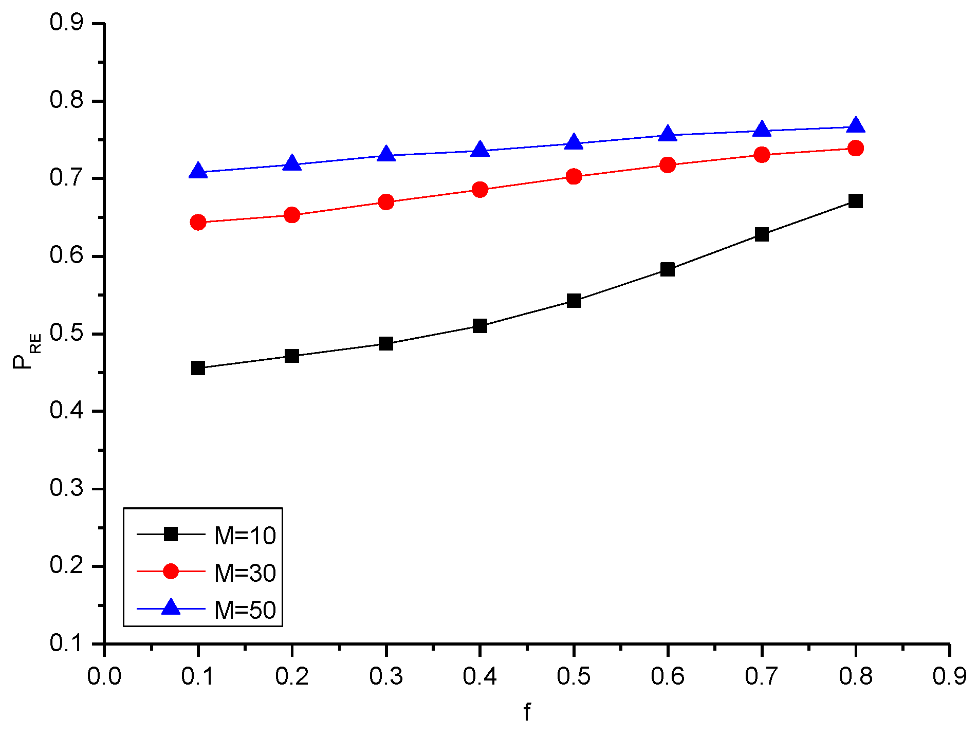
M/f	0.1	0.2	0.3	0.4	0.5	0.6	0.7	0.8
10	0.455	0.471	0.487	0.510	0.542	0.582	0.628	0.671
30	0.643	0.652	0.669	0.685	0.702	0.717	0.730	0.738
50	0.708	0.718	0.729	0.735	0.745	0.755	0.761	0.766

, the reconstruction error probability performance with N = 30 and m₀ = 2, for different number of networks M = 10, M = 30, and M = 50, is shown. Compared to the small-world network environment, the reconstruction error probability values are quite high even in low percentage of node failures for M = 30 and M = 50. Due to the complex topology of the scale-free network model, increase in M affects the link estimation ability of the MLPNN. Finally, Figure 11 and

Table 6. Probability of reconstruction error for scale-free networks with m₀ = 2, m₀ = 3, m₀ = 4, N = 30, and M = 10.

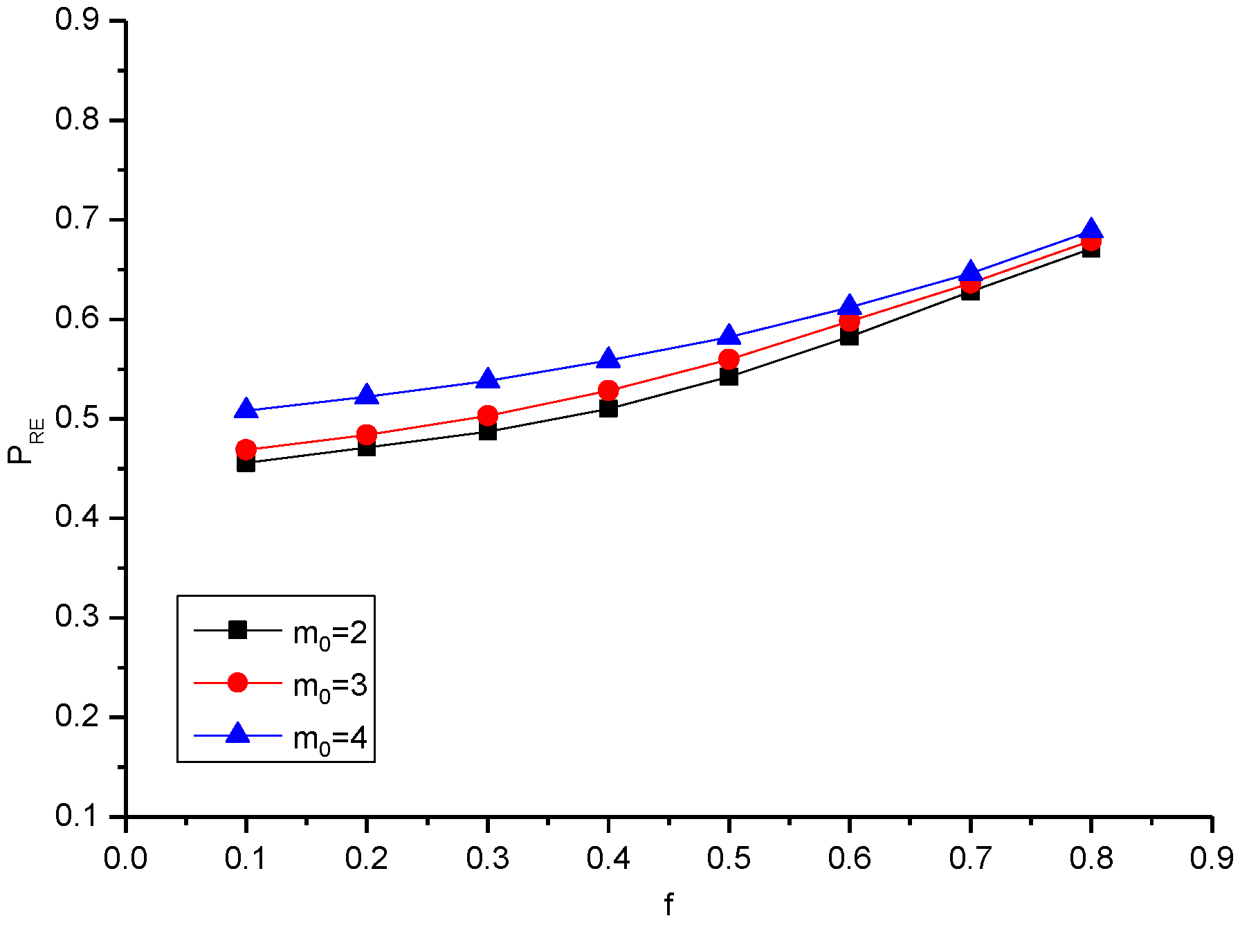
mo/f	0.1	0.2	0.3	0.4	0.5	0.6	0.7	0.8
2	0.455	0.471	0.487	0.510	0.542	0.582	0.628	0.671
3	0.468	0.483	0.503	0.528	0.559	0.597	0.636	0.679
4	0.508	0.522	0.530	0.558	0.582	0.612	0.646	0.689

shows the reconstruction accuracy performance with different initial number of nodes in constructing scale-free network model. One can observe that there is a small difference in reconstruction performance for high percentage of node failures, regardless of the initial number of nodes. This is because the link estimation difficulty is almost equal to the MLPNN, even if they have different degree distributions, when the number of hubs remains the same in scale-free networks.

5. Conclusions

In this paper, we proposed a new method that efficiently reconstructs the topology of the damaged complex networks based on NN technique. To the best of our knowledge, our proposed method is the first known attempt in the literature to recover the network topology after the network has been damaged and also the first known application of the NN technique for complex network optimization. The main purpose of our work was to design a NN solution based on known damaged network topology for accurate reconstruction. The proposed reconstruction method was evaluated based on the probability of reconstruction error in small-world network and scale-free network models. From simulation results, the proposed method was able to reconstruct around 70% of the network topology for 10% node failures for small-world networks and around 50% of the network topology for 10% node failures for scale-free networks. Important topics that need to be considered in the future work is to develop a new link list that can represent both unidirectional and bidirectional link information and various performance metric needs to be developed that can be used to provide deeper understanding on the network reconstruction performance.

References

- Wang, X.F.; Chen, G. Complex networks: Small-world, scale-free and beyond. IEEE Circuits Syst. Mag. 2003, 3, 6–20. [Google Scholar] [CrossRef]
- Newman, M. Networks: An Introduction; Oxford University Press: Oxford, UK, 2010. [Google Scholar]
- Sohn, I. Small-world and scale-free network models for IoT systems. Mob. Inf. Syst. 2017, 2017. [Google Scholar] [CrossRef]
- Barabási, A.; Albert, R. Emergence of scaling in random networks. Science 1999, 286, 509–512. [Google Scholar] [PubMed]
- Albert, R.; Barabási, A. Statistical mechanics of complex networks. Rev. Mod. Phys. 2002, 74, 47–97. [Google Scholar] [CrossRef]
- Barabási, A.L. Scale-free networks: A decade and beyond. Science 2009, 325, 412–413. [Google Scholar] [CrossRef] [PubMed]
- Crucitti, P.; Latora, V.; Marchiori, M.; Rapisarda, A. Error and attack tolerance of complex networks. Phys. A Stat. Mech. Appl. 2004, 340, 388–394. [Google Scholar] [CrossRef]
- Tanizawa, T.; Paul, G.; Cohen, R.; Havlin, S.; Stanley, H.E. Optimization of network robustness to waves of targeted and random attacks. Phys. Rev. E 2005, 71, 1–4. [Google Scholar] [CrossRef] [PubMed]
- Schneider, C.M.; Moreira, A.A.; Andrade, J.S.; Havlin, S.; Herrmann, H.J. Mitigation of malicious attacks on networks. Proc. Natl. Acad. Sci. USA 2011, 108, 3838–3841. [Google Scholar] [CrossRef] [PubMed]
- Ash, J.; Newth, D. Optimizing complex networks for resilience against cascading failure. Phys. A Stat. Mech. Appl. 2007, 380, 673–683. [Google Scholar] [CrossRef]
- Clauset, A.; Moore, C.; Newman, M.E.J. Hierarchical structure and the prediction of missing links in networks. Nature 2008, 453, 98–101. [Google Scholar] [CrossRef] [PubMed]
- Guimerà, R.; Sales-Pardo, M. Missing and spurious interactions and the reconstruction of complex networks. Proc. Natl. Acad. Sci. USA 2010, 106, 22073–22078. [Google Scholar] [CrossRef] [PubMed]
- Zeng, A. Inferring network topology via the propagation process. J. Stat. Mech. Theory Exp. 2013. [Google Scholar] [CrossRef]
- Haykin, S. Neural Networks: A Comprehensive Foundation; Macmillan: Basingstoke, UK, 1994. [Google Scholar]
- Zhang, M.; Diao, M.; Gao, L.; Liu, L. Neural networks for radar waveform recognition. Symmetry 2017, 9. [Google Scholar] [CrossRef]
- Lawrence, S.; Giles, C.L.; Tsoi, A.C.; Back, A.D. Face recognition: A convolutional neural-network approach. IEEE Trans. Neural Netw. 1997, 8, 98–113. [Google Scholar] [CrossRef] [PubMed]
- Lin, S.H.; Kung, S.Y.; Lin, L.J. Face recognition/detection by probabilistic decision-based neural network. IEEE Trans. Neural Netw. 1997, 8, 114–132. [Google Scholar] [PubMed]
- Fang, S.H.; Lin, T.N. Indoor location system based on discriminant-adaptive neural network in IEEE 802.11 environments. IEEE Trans. Neural Netw. 2008, 19, 1973–1978. [Google Scholar] [CrossRef] [PubMed]
- Sohn, I. Indoor localization based on multiple neural networks. J. Inst. Control Robot. Syst. 2015, 21, 378–384. [Google Scholar] [CrossRef]
- Sohn, I. A low complexity PAPR reduction scheme for OFDM systems via neural networks. IEEE Commun. Lett. 2014, 18, 225–228. [Google Scholar] [CrossRef]
- Sohn, I.; Kim, S.C. Neural network based simplified clipping and filtering technique for PAPR reduction of OFDM signals. IEEE Commun. Lett. 2015, 19, 1438–1441. [Google Scholar] [CrossRef]
- Watts, D.; Strogatz, S. Collective dynamics of ‘small-world’ network. Nature 1998, 393, 440–442. [Google Scholar] [CrossRef] [PubMed]
- Kleinberg, J.M. Navigation in a small world. Nature 2000, 406, 845. [Google Scholar] [CrossRef] [PubMed]
- Newman, M.E.J. Models of the small world. J. Stat. Phys. 2000, 101, 819–841. [Google Scholar] [CrossRef]
- Holme, P.; Kim, B.J.; Yoon, C.N.; Han, S.K. Attack vulnerability of complex networks. Phys. Rev. E 2002, 65, 1–14. [Google Scholar] [CrossRef] [PubMed]
- Johnson, J.; Picton, P. How to train a neural network: An introduction to the new computational paradigm. Complexity 1996, 1, 13–28. [Google Scholar] [CrossRef]
- Marquardt, D.W. An algorithm for least-squares estimation of nonlinear parameters. J. Soc. Ind. Appl. Math. 1963, 11, 431–441. [Google Scholar] [CrossRef]