Graph Cellular Automata with Relation-Based Neighbourhoods of Cells for Complex Systems Modelling: A Case of Traffic Simulation


Department of Computer Science, West Pomeranian University of Technology, 52 Żołnierska Str., 71-210 Szczecin, Poland
Symmetry 2017, 9(12), 322; https://doi.org/10.3390/sym9120322
Submission received: 5 December 2017
/
Revised: 5 December 2017
/
Accepted: 17 December 2017
/
Published: 19 December 2017
Abstract
:A complex system is a set of mutually interacting elements for which it is possible to construct a mathematical model. This article focuses on the cellular automata theory and the graph theory in order to compare various types of cellular automata and to analyse applications of graph structures together with cellular automata. It proposes a graph cellular automaton with a variable configuration of cells and relation-based neighbourhoods (r–GCA). The developed mechanism enables modelling of phenomena found in complex systems (e.g., transport networks, urban logistics, social networks) taking into account the interaction between the existing objects. As an implementation example, modelling of moving vehicles has been made and r–GCA was compared to the other cellular automata models simulating the road traffic and used in the computer simulation process.
1. Introduction
Cellular automata (CA), described by cell structure, rules and possible states, are mathematical models functioning as a modelling environment for discrete systems. Works on CA development were started in the 1940s by John von Neumann and Stanisław Ulam and then classified and discussed by Wolfram [1].
CA development led to the creation of many types and implementations of both homogeneous and nonhomogeneous, structurally dynamic [2,3], asynchronous automata designed to explore the processes taking place in the real world [4,5], and graph automata, nonhomogeneous on the grounds of the different cardinality of the neighbourhood of individual cells [6,7,8].
The CA-related literature analysis has led to the conclusions presented in Table 1.
CA utilizing graphs for describing neighbourhood models have inspired the author to go beyond the spatial analysis and GIS systems. A task has been set to generalize CA so as to allow for system modelling in virtual spaces (e.g., transport networks, connection networks, etc.). In this article, a structurally dynamic relative neighbourhood cellular automaton is described. In order to define it, after a short presentation of the CA definition, a reconfigurable graph acting as a tool for describing the modelled objects (system elements) and their relative neighbourhoods will be discussed. Next, a graph cellular automaton (r–GCA) will be presented, along with the possibilities of its implementation in defined systems, as sets of the same type related objects.
As a computational example, traffic simulations will be demonstrated along with a comparison of the efficiency of the developed structure with the other CA models of traffic dynamics.
2. Related Work
Cellular automata (CA) [9,10,11] are models of physical systems where time and space are discrete and interactions are local. They have been used as models for complex systems and have also been applied to different kind of problems [12,13,14,15,16,17]. As Toffoli and Margolus wrote, CA are the computer scientist’s counterpart to the physicist’s concept of “field” [18]. Researchers have attempted to classify CA both in the general aspect [1,19,20] and directed to certain criteria [21,22].
Many authors use CA to model and simulate selected phenomena associated with various areas of life, i.e., mathematics, physics, engineering and transport. Besides these applications, the lattice grid of cellular automata has been providing a by-product interface to generate graphical contents for digital art creation. Javid et al. [23] indicate that one important aspect of cellular automata is symmetry, detecting of which is often a difficult task and computationally expensive. Authors present a swarm intelligence algorithm as a tool to identify points of symmetry in the cellular automata-generated patterns.
In the classic sense, CA are a network of cells that are adjacent to each other and exhibit some interactions. In this case, the definition of neighbourhood is very straightforward. The most usual types of neighbourhood definition are known as Von Neumann and Moore neighbourhoods, which consider some or all of the cells adjacent to a given cell. These neighbourhoods can also be extended using a radius around the central cell. Another kind of neighbourhood was proposed by Hoffmann et al. [24], where the cell state consists of a data field and additional pointers. Via these pointers, each cell has read access to any other cell in the cell field, and the pointers may be changed from generation to generation. Compared to the classical CA the neighbourhood is dynamic and differs from cell to cell.
The problem of neighbourhood becomes more complex in irregular spaces, such as in subjects connected to adaptability of urban spaces or land use change [25,26,27,28,29]. For example, Dahal and Chow [30] proposed neighbourhood definition based on topological relations and the extended neighbourhood, in which the entire study area is considered the neighbourhood of every urban parcel. O’Sullivan in [8] presented a new type of a dynamic spatial model: graph cellular automaton (graph-CA). The author has shown that a graph cellular automaton with specific structural properties defined in the relations between the subsets of cells is a useful generalisation of the traditional cellular automaton. Moreover, the author argues that deriving a graph cellular automaton both from a graph and from formalism of a cellular automaton enables simultaneous application of well-developed methods of describing the model structure and the process dynamics. Geospatial division of land plots served as an example. With the aim of realistic representation of the land use, the authors of the article [31] presented a prototype of the method based on graph cellular automata. The method effectiveness was checked using the example of one of the dynamically developing municipalities of Madrid. The authors have shown that the graph structures applied to describe the districts of varied surfaces operate within reasonable computation time.
Roka [32] presents generalisation of cellular automata to the cellular automata specified in Cayley graphs. Several sufficient conditions were provided for a cellular automaton to be able to be stimulated by a one-way cellular automaton which has the same basic graph. Unfortunately, the works on OCA (one-way Cellular Automaton) have not been fully completed.
An interesting approach was proposed in [33]. The authors checked the impact of the topology variation on the dynamic behaviour of the system with local updates of the rules. One-dimension, binary cellular automata were implemented on graphs showing different topologies via formulation of two sets of degree-dependant rules, out of which each contains one parameter. The authors observed that the graph topology changes cause transitions between various dynamic domains without a formal change in the update rule. The article discusses implications in the context of information transmission in complex network systems.
Another application was presented in [34], where a graph-based cellular automaton was developed in order to simulate the surface flows on the plains. As opposed to the classical cellular automata represented by a network of cells, the presented model is served by a graph structure which ensures more flexibility in order to describe the complex geographic domains of different scales. The model computes the flow of water between the adjacent cells on the basis of hydraulic equations assigned to the arcs of the graph. Comparing the results of the hydraulic measurements taken during flood events has shown a perfect compliance of the presented model. The earlier works in that regard were implemented by the authors using classical cellular automata [35].
Many other CA implementations based on graphs have been made [36,37,38,39,40] but these implementations are not directed at studying the relationship between CA cells.
The algorithm, based on the graph cellular automaton concept, was proposed in [41] for solving the lifetime coverage problem (MLCP) in wireless sensor networks (WSN). The authors recommend that the discussed algorithm should have all the advantages of the located algorithm, i.e., exclusively on the basis of knowing the neighbours, it may reorganise the WSN, preserving the required coverage ratio, and thus extending the life of the WSN. The simulation results are the first in the series and they show that the developed algorithm obtains results that are similar to those generated by the centralised algorithm in relation to lifetime (q) metric.
The graph-CA-based approach to the analysis of social networks and connections between users who are far away but close in the relationship of common friends, common interests, etc. is presented in [42]. Empirical studies were based on data sets from social platforms, which confirmed effectiveness of the proposed solution.
As can be inferred from the above, many attempts have been made to connect the graph theory with the cellular automata theory. Usefulness of such a concept has been proved for many applications. However, none of these studies has been continued in the field of traffic modeling. The neighbourhood is still treated here as a physical neighbourhood of the two closest cells of the CA. However, besides direct dependence, we can also observe an indirect dependence. For example, a vehicle being far (several vehicles) in front of the analysed vehicle will suddenly slow down or suddenly stop, and knowledge of this could reach the analyzed vehicle earlier than only through the direct dependence of subsequent vehicles (in fact, sometimes several vehicles are involved in the collision). Another example, the light at the intersection changes to red. Previous models react sequentially by braking individual vehicles. In fact, the driver in the queue of vehicles approaching the intersection sees the changing signaling light and reacts a bit earlier, e.g., through further idling, which may lead to fuel economy and thus to reduce environmental pollution. Therefore, it is worth taking up the extension of existing models with the idea of a dependency neighbourhood (hereinafter referred to as the relational neighbourhood) to make the simulation more realistic.
This article formalises the research conducted by the author with the aim of developing a graph cellular automaton for modelling and simulation of complex systems, with special focus on traffic simulation. The author introduced the concept of relation-based neighbourhoods graph-based CA (r-GCA). This concept helps in the modeling of processes whose elements are interdependent despite the lack of physical dependence (mutual proximity).
3. Proposed Approach
The chapter is divided into the following parts. First, the idea of the classical CA was outlined, followed by the elements leading to development of graph cellular automaton with relation-based neighbourhoods, varying over time. On that basis, as an example of application, a model of a graph cellular automaton for traffic modelling was developed. The experimental research regarding the model is shown in the next chapter.
3.1. Classic Definition of Cellular Automata
Classic CA defined as CA = (, , ) is described by [43]:
- Cell grid in d-dimensional space (d ≥ 1);
- Automaton state, dependent on sets of states of individual cells;
- rule defining cell state at time t + 1 dependent on the state of this cell and its neighbourhood at time t;
- Classic (homogenous) CA is characterized by:
- ○
- identical set of states for each cell;
- ○
- identical set of rules (identical for the entire grid;
- ○
- automaton grid not changing over time;
- ○
- identical neighbourhood diagram for the entire grid.
If at least one of the aforementioned characteristics is not true, a CA is not classic, or, in other words, it is nonhomogeneous.
3.2. Graph Changing over Time
In order to define a relative neighbourhood cellular automaton, a formal description of neighbourhoods in graphs will be presented. An additional virtue of the described graph is the dynamic cell configuration.
Let us consider a directed weighted graph:
defined by a set of nodes (hereinafter vertices) , edges , set of weights K and edge weight function α.
Edges E of graph are defined as a Cartesian square:
while , which dictates that a graph is not a directed graph.
Function α (weight function) defines weights of edges of graph :
where or, more generally speaking, . Weights are values that indicate the significance of the connection between the vertices. In systems where there are many vertices connected to each other, not all have the same priority. For example, in the real world, crossing the road from one city to another may require a certain amount of time or energy; in the virtual world (in social networks) users have different “friends” but the user does not have the same relationship with each of them.
The neighbourhood of vertex is a set of vertices connected to vertex by edges from set of graph . Neighborhood of a directed graph comprises a sum of sets of neighborhoods connected by out-edges and in-edges of vertex :
where ,
A sets of weights of in-edges and out-edges of a graph for neighbourhoods are a sets of such edge weights or that belong to a set of weights and at the same time the edge that is described by the weight belongs to the set of edges of the graph . They can be defined as:
A neighbourhood can be defined by a neighbourhood matrix and weights of directed edges can be written as a weight matrix. Matrices are structures that can be easily implemented in the form of a computer program and they can store the information. If the graph has n vertices, the neighbourhood matrix of n x n size is built as presented:
where for , for .
For this graph, weighted neighbourhood matrix of n x n size includes weight coefficients of individual edges of the directed graph:
where , , .
The number of neighbours of vertex is defined by its degree: ) = ||. A vertex can be isolated in , when ) = 0. If ) = 1, then the vertex is called a leaf of the graph. Minimal and maximal degrees of graph are defined as:
3.3. Change of Graph Structure
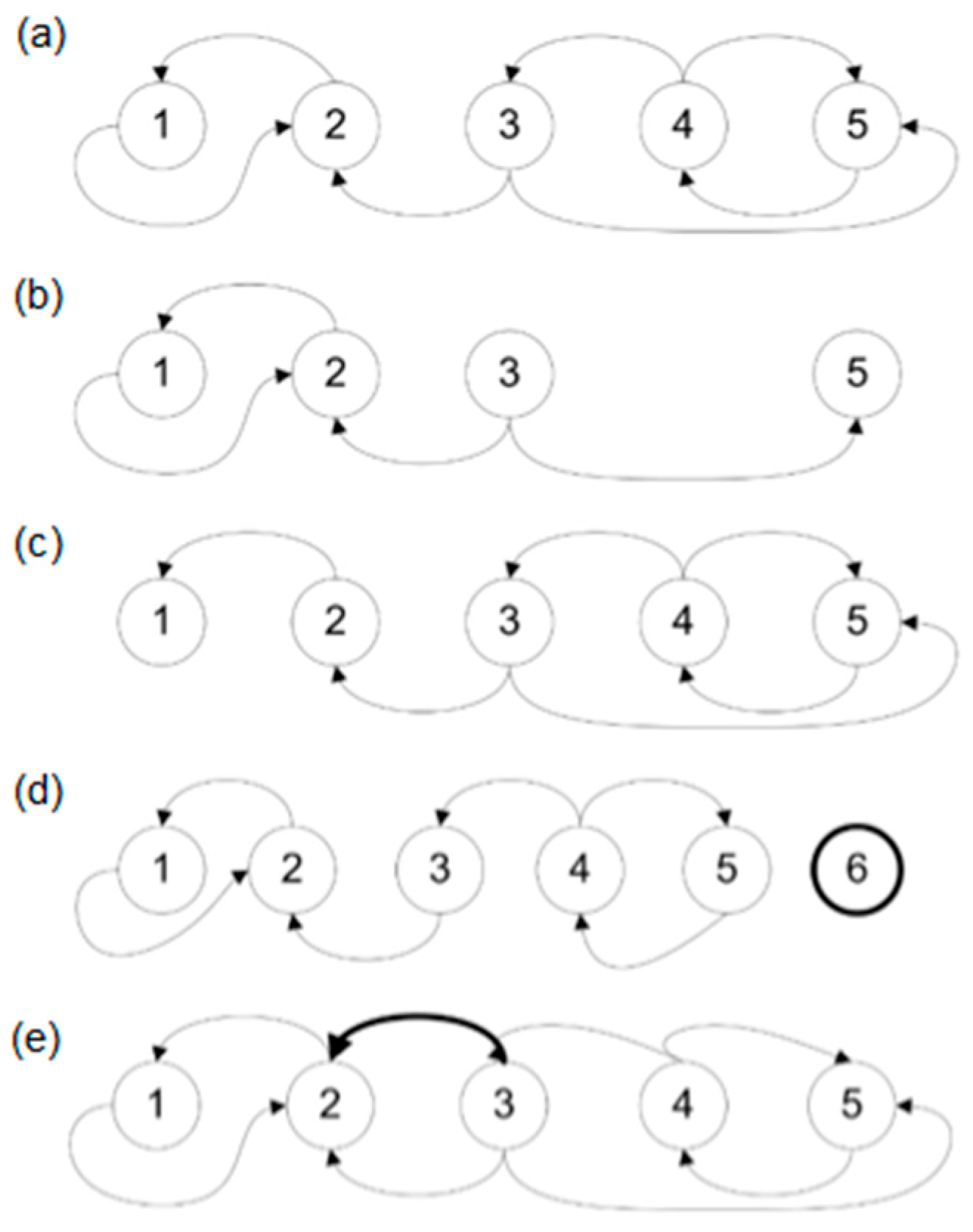
In this part, the possible graph transformations have been described. All transformations are shown in Figure 1 and defined in the following subsections. In complex systems, the structure of the graph describing the system is constantly changing, hence the need to perform operations related to removing the graph edges, deleting the graph vertices, and adding edges and vertices to the graph.
3.3.1. Removing Vertices from Graph
Removing vertices from graph results in an induced subgraph . The subgraph is a graph whose vertices set is a subset of the set of vertices of graph , and the set of edges consists of all edges of graph whose ends belong to the set of vertices of the newly formed graph. The set of vertices of this subgraph cannot be empty. Let us define a function allowing for the removal of vertices accordingly:
where is the difference between the set of all vertices of the graph and the set of deleted vertices and is the set of all edges of the vertices of graph that have not been removed:
Removal of vertices results in simultaneous removal of related edges. If , then .
3.3.2. Removing Edges from Graph
Removing edges from graph G results in an induced subgraph .
Let us define a function allowing for the removal of edges :
where is the difference between the set of all edges of the graph and the set of deleted edges :
On the level of vertex it is possible to define a local edge removal function as (a):
where or (b):
where .
3.3.3. Adding Vertices to Graph
Let us define a function allowing for the addition of vertices :
where is the sum of the set of all vertices of the graph and the set of added vertices :
This operation does not create edges, so the new vertices are isolated in .
3.3.4. Adding Edges
Let us define a function allowing for the addition of edges :
For the set, the addition of vertices to graph can be written as:
On the level of vertex it is possible to define a local edge addition function as (a):
where or (b):
where .
Among the aforementioned functions, global transformations can be found causing changes of the entire directed graph:
- —removing vertices defined by set;
- —removing edges defined by set;
- —adding vertices defined by set;
- —adding edges defined by set.
Local transformations related to the changes of graph edges:
- —removing out-edge ;
- —removing in-edge ;
- —adding out-edge ;
- —adding in-edge .
3.3.5. Reconfigurability of Graph over Time
A change of global graph configuration can be defined by a function of global graph reconfiguration:
which is defined as a combination of few functions dependent on each other:
so:
where is a set of vertices deleted from graph , is a set of vertices added to graph , and are sets of edges, respectively, deleted and added to graph . If then . If for each t and t + 1 an equation is true, then the graph is not reconfigurable over time.
When the configuration of the graph changes, a new graph is created which may differ from the previous one by the number of vertices, edges, and weights. This kind of reconfiguration of the graph constitutes the basis for the neighbourhood in the following new graph cellular automaton.
3.4. Relative Neighbourhood Structurally Dynamic Graph Cellular Automaton
Let us define a structurally dynamic relative neighbourhood graph cellular automaton (r–GCA), as:
where:
- d—dimension in a d-dimensional space (d ≥ 1) representing cell grid;
- —activity state of an automaton, dependent on the set of activity states of individual cells;
- —state of automaton, dependent on the set of states of individual cells;
- —directed weighted graph defined above;
- is a function defining the state of automaton cell at time t + 1 dependent on the state of this cell and its neighborhood at time t;
- is a global rule defining the conditions of activation or deactivation of cellular automaton cells and the rules of graph reconfiguration (defines sets of added and removed by vertices and edges of graph G), depends on the automaton state (states of all cells);
- is a function of reconfiguration of graph and cells activation/deactivation based on conditions set by .
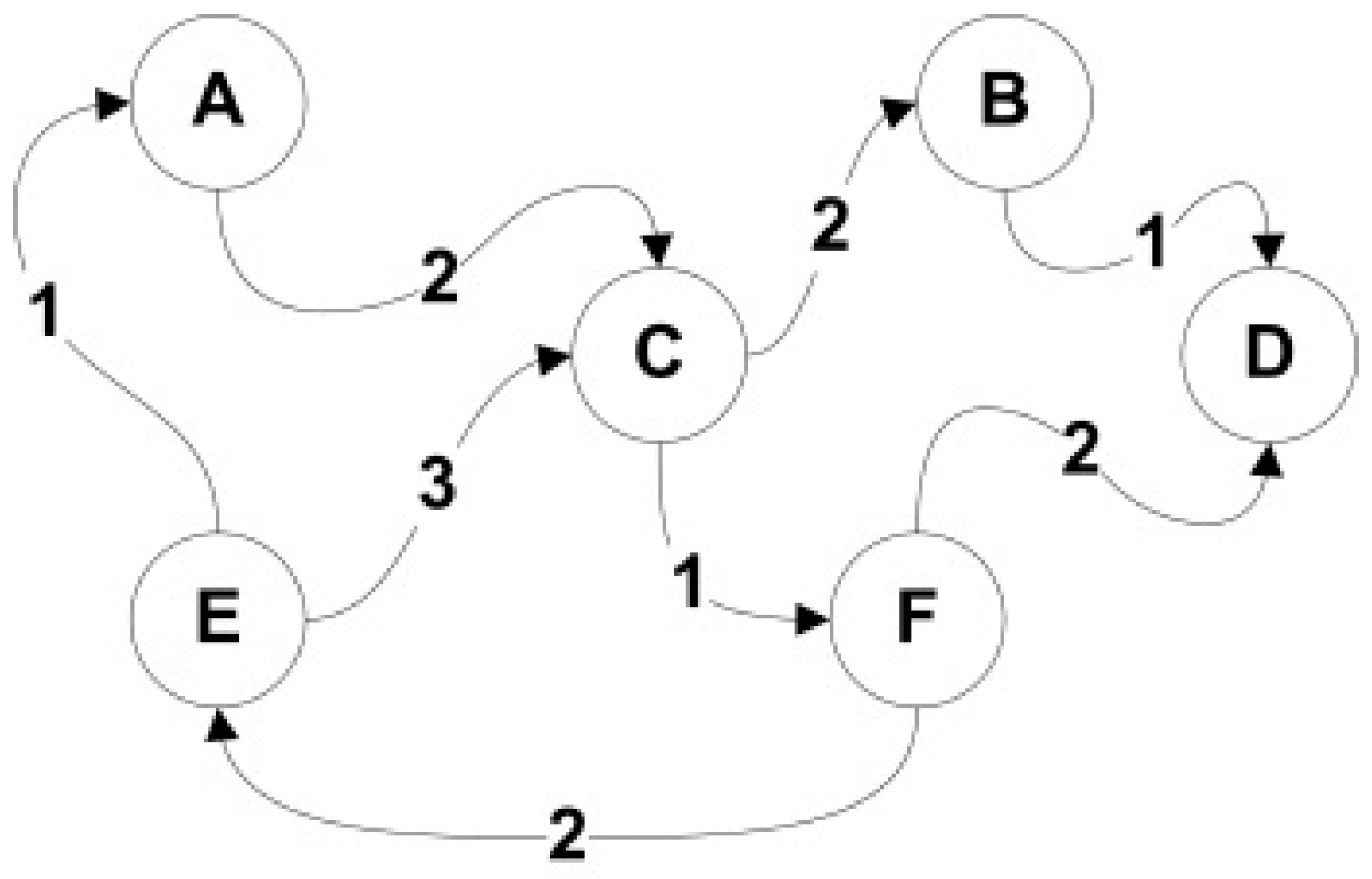
The automaton is defined by a directed weighted graph and automaton state (at time t), which means that each graph vertex corresponds to one automaton cell. A cell neighbourhood of this cellular automaton is defined by graph edges belonging to the vertex set, meaning for every neighborhood exists, described by out-edges and in-edges of this vertex. Figure 2 presents the example of graph .
Local rule depends on the state of cell described by a graph and states of adjacent cells defined by neighborhood and the influence of those neighborhoods expressed by weights of graph edges describing each individual neighbourhood of .
In general:
The proposed model, unlike the classical CA, uses a dynamically changing relational neighbourhood. The classically-understood neighbourhood in CA is the relationship between cells located in a direct environment in a d-dimensional space (CA cells grid). It is related to the regular arrangement of the CA cell in the space. In such CA, the state of the cell is influenced by neighbouring cells in its environment, eg von Neumann or Moore’s neighbourhood.
In the case of r–GCA, the dimension d no longer has the same meaning as in the classical CA, but it is still relevant for model implementation, e.g., in Field-Programmable Gate Array (FPGA) structures or in the form of a computer program. In the proposed r–GCA, this kind of neighbourhood is called a physical neighbourhood and defines the structure of the regular cell grid selected at the implementation stage. Contrary to the classical CA, a defined neighbourhood does not affect the state of a given cell. In the proposed r–GCA, the cell state is also determined on the basis of its state and the states and relationships of neighbouring cells, but in this case the neighbourhood is defined by graph. The neighbourhood has logical character: relationships belong to a set of relations (corresponding to the weights of the graph’s edge) and are not dependent on the position of the cells in the cell grid. Due to its nature, the logical connection is called the relational neighbourhood.
Specifically, such a relation can be:
- any relation between objects represented by graph vertices (e.g., interdependence of vehicles on the road, interdependence of members of a project team in a computer project, relations between people in this group or types of relations between people connected to a social network);
- the distance between objects represented by graph vertices;
So, unlike in case of regular neighbourhood homogeneous cellular automata, in the presented approach there are two types of neighbourhood:
- physical—automaton cell neighbourhood in d-dimensional space;
- logical—a set of relative neighbourhoods defined by a reconfigurable graph (which allows for modeling a system of dynamic number of objects).
For example, the relations of objects of the modelled system using r–GCA and described by the graph which was presented in Figure 2 correspond to the six cells (A, B, ..., F) of this automaton. These may be any cells from the d-dimensional grid of cells (e.g., from the two-dimensional grid of the CA shown in Figure 3). In this case, we deal with three types of relations defined by weights from the set .
A dynamic number of system objects can be modelled with r–GCA thanks to the activation and deactivation mechanisms of individual cells. In d space, only the cells corresponding to graph vertices are active:
Activity of automaton depends on the set of activity states of individual cells.
Compared to the homogeneous (classic) cellular automata, here the rule is present as well, related to the cell structure configuration and neighbourhood. The initial cell structure configuration can change over time through:
- activation of inactive cells (which equals to addition of related vertices to the graph);
- deactivation of cells (which equals to removal of graph vertices and edges connected to them);
- adding or removing graph edges, which results in creation or removal of neighbourhood relations.
3.5. Representation in the Computer
The most popular methods of representing graphs in the computer memory include the neighbourhood matrix, incidence matrix and neighbourhood list. The above-mentioned methods share one common feature: tables which are used for recording the data on the vertices and the edges between them.
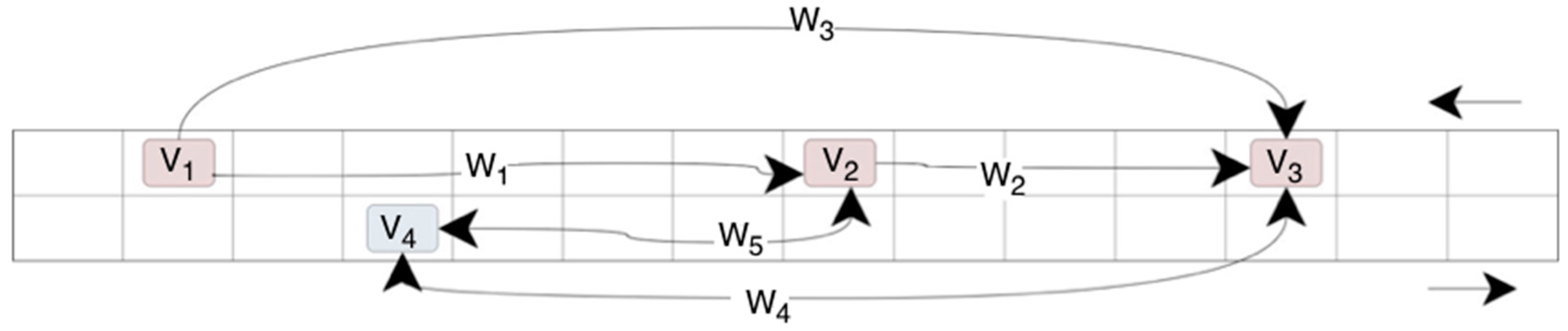
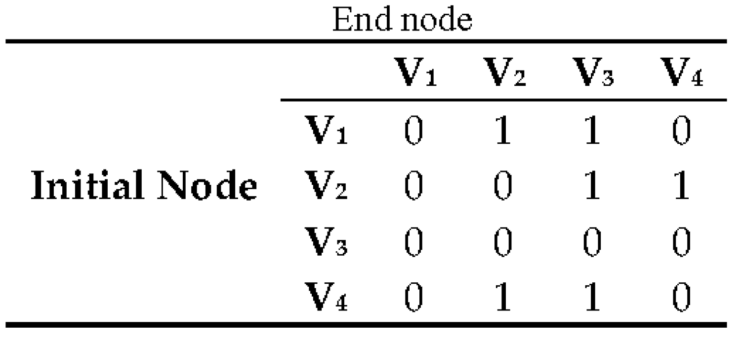
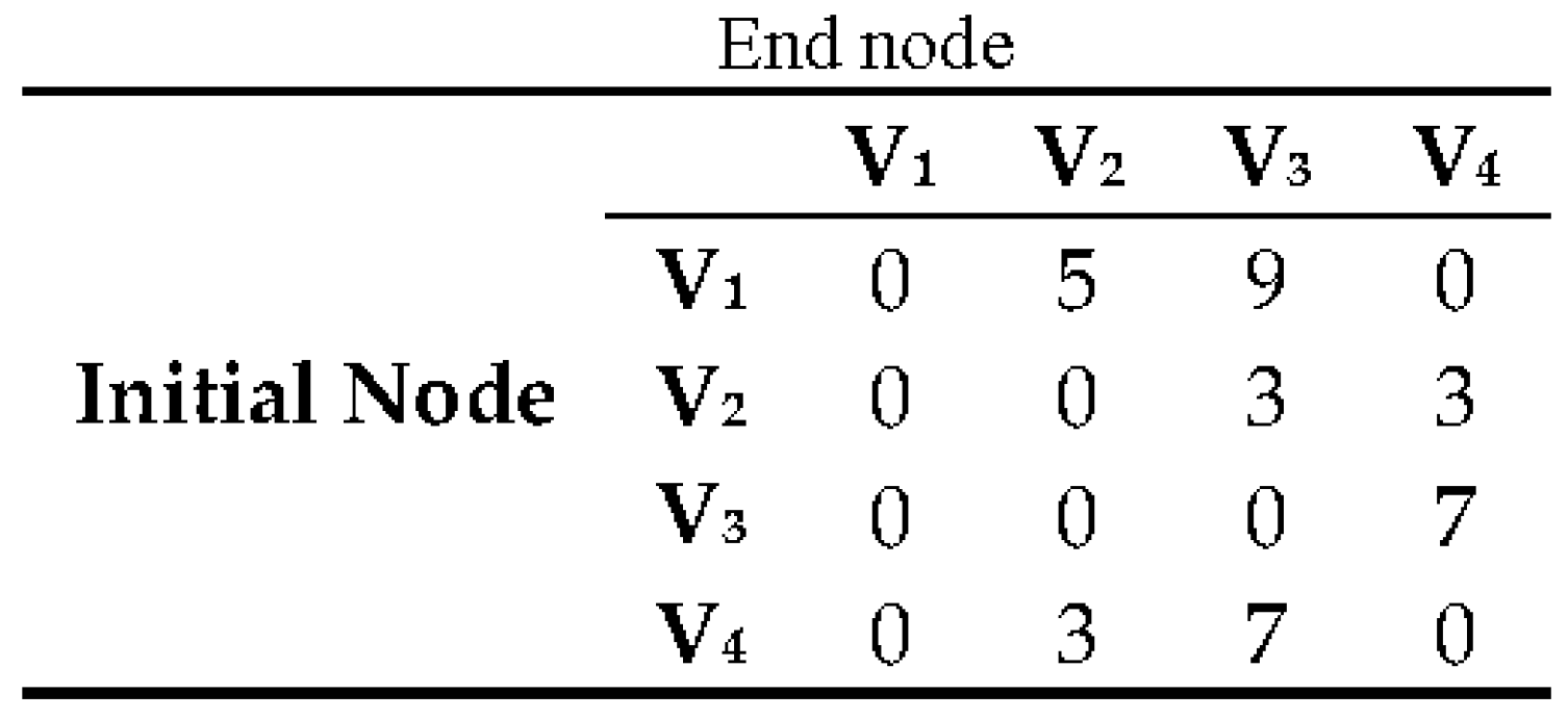
The neighbourhood matrix [44] is a square matrix, whose grade indicates the number of graph vertices. The lines correspond the initial vertices, and columns—the end vertices of the graph. Figure 4 presents a graph consisting of three vertices , two edges and . Edge does not exist: it was shown only to demonstrate the mapping in the neighbourhood matrix. Simultaneously, this figure is an example of a directed graph (if there is an edge from vertex to there is no edge in the opposite direction), therefore it is possible to express the dependence with symbols:
where: —neighbourhood matrix, —matrix line, —matrix column.
In order to check if there is an edge between vertex and it is necessary to check in the neighbourhood matrix if there is value 1 in line and column . If so, the edge exists. The complexity class for matrix with vertices is fixed and amounts to whereas its drawback is the class of memory occupancy class which is . A lot of significant information can be derived from the neighbourhood matrix (Figure 4), for example, the vertex grade in the directed graph, which can be done by summing up a given line. Vertices and are connected if .
In the proposed approach, the neighbourhood matrix and matrix of weights (presented in next part) were used in order to describe the situation in the dynamic vehicle traffic on a two-way street.
4. The Case Study—Traffic Simulation
4.1. Existing Traffic Models
In 1992, Nagel and Schreckenberg [45] developed a model of traffic dynamics in the form of a cellular automaton. The authors formulated a stochastic discrete cellular automaton model for one-lane roads, divided into parts of 7.5 m long (hereinafter referred to as CA cells). The developed microscopic model assumes that time and space are discretized and that through low computational complexity the model can be used to model large numbers of vehicles [46].
The single lane model (N-Sch) can clearly express the vehicle traffic flow situation in the same direction one-lane, but this model has the limitation of not including overtaking and this model proved that a strictly deterministic model is not realistic. Researchers began work on other models [47,48,49,50,51] and two-lane traffic model [52] and later on traffic heterogeneity [53,54]. However, in the case of the two-line model, the lack of stochasticity causes strange behaviors of the group of vehicles on one of the two lanes. When individual vehicles do not get to maximum speed, the whole group changes lanes, and this happens several times until the group of vehicles is diluted or when the whole group passes alongside other vehicles. Rickert et al. [55] have introduced the stochasticity into the two-lane rule set and thus the effective number of lane changes has been reduced. The simulation revealed that the effect of stochasticity is also important in the asymmetric free–flow case. Rickert et al. have assumed two kinds of criteria (incentive and safety) as a symmetric rule set for traffic flow with cars which change lanes. Chowdhury and Wolf [56] proposed the STCA (symmetric two-lane cellular automata) traffic flow model with two kinds of vehicles. The lane-changing rules can be symmetric or asymmetric with respect to the lanes and to the cars [57]. The symmetric model is interesting for theoretical considerations whereas the asymmetric model is more realistic. In general, it seems that the approach to multi lane traffic using simple discrete models is a useful one for understanding fundamental relations between microscopic rules and macroscopic measurements.
The main basis of the lane-changing rule in STCA traffic flow model is that the lane-changing distance must be fixed. However, this is not appropriate in the actual traffic flow. Based on the STCA model, a new F-STCA (flexible STCA) model was proposed which is a cellular automata traffic flow model based on the safe lane-changing rule [58,59]. This model considers the influence of the rear vehicle in the adjacent lane and can simulate the actual traffic flow situation a bit better. However, in actual traffic flow, when the driver decides to change lanes, he should not only consider the influence from the rear vehicle in the adjacent lane, but also consider the influence from the front vehicle in the adjacent lane. Xu and Zhang [60] have proposed model based on an improved safe lane-changing distance constraint rule. However, the risk value of lane-changing is only for specific circumstances; it is not universal. Xu and Xu [61] have considered the possible conflict between the lane-changing vehicle and the rear vehicle or front vehicle in the adjacent lane and they presented a symmetric same direction two-lane traffic flow model (hereinafter referred to as X-STCA).
The N-Sch model proved to be a powerful and simple road traffic simulation tool and it began various modifications and extensions [62,63,64,65,66,67,68,69,70,71], but all these new solutions are based on direct neighbourhood (neighbouring, closest cells) and they are focused mostly on one-way roads.
4.2. Traffic Model on the Basis of a Graph Cellular Automaton
The author proposes a solution that preserves the idea presented in above-mentioned models based on the N-Sch model but with a different representation. The dependencies resulting from the earlier CA are maintained, but a graph representation has been used to better map the neighborhood dependency. Vehicles are represented as graph nodes and the relationships between vehicles are represented as neighbourhood matrix and matrix of weights. Such representation implies the ability to continue using the already developed mechanisms such as the traveling salesman problem or vehicle routing problem.
To understand the idea of the presented approach, a fragment of a two-way road with moving vehicles is presented (Figure 5). The interdependence of the vehicles was shown by means of arrows and presented in the form of a graph in Figure 6. If the edge between the graph vertices has arrowheads on both ends, both vehicles interact. If the edge between the vertices has one arrowhead, then the vehicle (the vertex without an arrowhead) affects the other vehicle (the vertex with an arrowhead). Therefore, the edge with one arrowhead will be a fragment of a directed graph, and the edge with two arrowheads will be a fragment of an undirected graph.
In the further part, a neighbourhood matrix and a matrix of weights were created. The matrix of weights contains information on the distances between the interdependent vehicles. The distances are measured in the CA cells. Neighbours of a given vehicle are the vehicles located in front of it in the same lane, as well as the vehicles in the other lane moving in the opposite direction. Moreover, a rule was established that the vehicles which have already passed each other no longer affect one another.
As for the example shown in Figure 5 and Figure 6, the matrices of neighbourhood and weights take the form presented in Figure 7 and Figure 8.
The simulation of the vehicle traffic is based on the analysis of the neighbourhood matrix (Figure 7) and the matrix of weights (Figure 8).
The individual stages of the transition function, in the developed model for two-way traffic motion, are presented by means of a description and the general mathematical formulas. The function is understood to be a function of changing the state of CA cell (from t to t + 1) depending on the state of neighbours. In this case, this function is implemented in the following steps:
- Acceleration—if the vehicle did not reach maximum velocity and the weight of the vehicle in front of it is greater than its velocity, and also than the maximum velocity—then it can increase its velocity. This stage of the model can be presented as follows:
- ○
- if then , where the symbol is a value assignment operation, is a car velocity, is a maximum possible velocity, is a weight of the vehicle in front of analyzed one, on the same lane of road.
- Overtaking—if the vehicle was not able to accelerate due to the preceding vehicle and its velocity was less than the maximum velocity, and the vehicles approaching from the opposite direction (on the other lane) are at a far distance:
- ○
- if then the car can start overtaking (a procedure “overtake”), where W is a relation neibourhood (from matrix of weights) of car being on another lane of the road and going from the opposite; —a number of lanes of analysed vehicles and for the opposite one; i,l are number of CA cells of the analysed vehicle and for the opposite one.
- ○
- The procedure “overtake” consists of few stages: analysis of weights from the matrix of weights for analyzed vehicles, lane changing (), acceleration (above step) and overtaking of vehicle or vehicles and return to the original lane ().
- ○
- The computations necessary for overtaking include establishing the weights of the vehicles located in front of the given vehicle and searching for the smallest weight in the opposite lane. In the first place, an analysis of the opposite lane is performed. The weights on the lane in front of the vehicle are sorted from the smallest to the greatest. Figure 9 presents the aim of sorting the weights in the context of a possibility to overtake any individual vehicles. Vehicle could overtake the vehicles driving in front of it. The analysis of weights enables checking the possibility of overtaking as many vehicles as possible. In case there is no such possibility, possible spaces between the vehicles are searched for.
- Braking—if the vehicle cannot accelerate, it cannot overtake, and if there are other vehicles in front of it, then it is forced to decrease its speed;
- ○
- if then , where is the nearest neighbour in the front of vehicle on the lane .
- Random events—each vehicle may (at some probability) decrease its velocity without a reason found in front of the vehicle (random reduction of speed by 1):
- ○
- if then , where is a probability of random event and is a random variable uniformly distributed over (0,1).
- Shifting—each of above steps additionally includes moving the vehicle to a new position: .
Let us consider from Equation (23) for the traffic case. Generally, it is a global rule defining the conditions of activation or deactivation of cellular automaton cells and the rules of graph reconfiguration (defines sets of added and removed by vertices and edges of graph G. In the analysed case, it can be understood as a collection of possible modifications of the situation on the road. The situation on the road changes over time. Vehicles appear on the road from the side roads, they leave the road to park or to other roads, they overtake each other, they brake and accelerate, they come closer or separate from each other, etc. Thus, each motion generates a need for changes in the graph describing the area and the vehicles in that area. This need to change is set over time (each iteration). The list of graph modifications (needs) specified by is than processed by function .
Thus, the function can be understood as all possible modifications of graph which were described in Section 3.3.1, Section 3.3.2, Section 3.3.3, Section 3.3.4 and Section 3.3.5.
The model presented above is unique due to the use of a relational neighborhood for the first time. The novelty is the inclusion of dependencies in the graph (neighborhood matrix and weight matrix) in the analysis of vehicle traffic, in particular in the overtaking procedure. Existing models have a lane change function, but they do not overtake several vehicles at the same time. In reality, however, such behaviors can be noticed and, to make the simulation process more realistic in the developed model, such behavior can be mapped based on the relational neighborhood.
4.3. Experimental Results
The stochastic nature of road traffic and its complexity allows for the application of a graph cellular automaton with relation-based neighbourhoods. The interdependence of vehicles travelling on the road is considerable and not always direct (many times, the interdependence is indirect due to other traffic participants separated from one another by several vehicles). Additionally, the traffic dynamics are considerable and require continuous reconfiguration of the model, in this case the graph structure. It is worth mentioning that the graph structure is used to describe the situation on the road, and the idea of the cellular automaton has contributed to application of simple transformation rules. In order to verify correctness of the model, the values were compared against those obtained in the course of road traffic simulations based on a classical cellular automaton.
The verification experiments (Figures 11–14) were run for the probability of a random event at the level of 0.3 and for varied road lengths expressed as a quantity of CA cells, and different numbers of vehicles. The number of vehicles was changed within the range from 50 to 1000, whereas the road length was changed within the range from 50 to 1000 CA cells. The simulations for each of the initial settings were run 20 times, and the average result was presented in Figures 11–14 which presents the comparative studies for the developed model (r–GCA) and the other CA models. Simulation 1 describes the case of 50 vehicles on a road 375 m long (50 cells), Simulation 2 involves 50 vehicles on a road of 500 cells (3750 m), simulation 3–500 vehicles and a road of 500 CA cells (3750 m), Simulation 4–500 vehicles, with a road of 1000 CA cells (7500 m), Simulation 5–1000 vehicles, with a road of 1000 CA cells (7500 m).
The experimental studies were performed using a computer with the following parameters: Intel Core 2 Duo T7500 (2.2 GHz) 4 MB, FSB 800 MHz, 4096 MB DDR2, 667 MHz SO-DIMM (2 × 2048 MB), SSD with SATA II. The developed software consists of two modules—the computation module and the visualisation module. The visualisation module is used for presenting the results of the computation module and communication with the user. The visualisation module was implemented in the library Allegro 5. The whole code was written in C++ using the Microsoft Visual Studio 2015 suite. The graph cellular automaton model (r–GCA) and other models were implemented in the computation module.
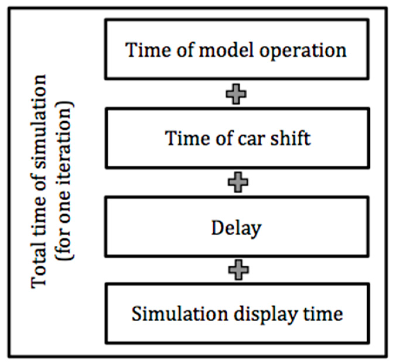
The simulation operation time is explained in Figure 10. Differentiation between the individual elements was useful for the purposes of detailed comparison of the analysed models. The total time of one iteration of the simulation consists of the time of the model operation (recomputing the vehicles positions, creating the graph, etc.), the time needed for the vehicle shift, the processor lag (forcing a break in the processor operation so as to reduce the operation temperature and thus to increase the simulation effectiveness) and the time of displaying elements on the computer screen. The operation lag was set to be 0.0025 s, which enabled the most fluent simulation.
Figure 11 and Figure 12 show the comparison of the vehicles’ average speeds in the simulation process for various road lengths and different numbers of vehicles. All models obtained comparable values, which is a correct comparative result showing that the developed model does not diverge from the other traffic models.
A slight difference may be noticed in Figure 12, in which the developed r–GCA model caused the simulated vehicles to obtain greater maximum speeds. This was due to the more realistic overtaking stage, in which a greater space in front of the vehicle is analysed (r–GCA model), as opposed other models where only the direct neighbourhood was analysed.
Then, the simulation operation times were compared. Figure 13 shows the comparative results of the total simulation operation time, where the other models were shown to work faster, particularly in the case of simulations involving a large number of vehicles (above 500). This is due to the time-consuming graph creation and transformation in the process of the overtaking and passing stage analysis.
The other times (displaying time, vehicle shift time, etc.) are practically the same for various analysed cases and, to a large degree, they depend on the applied IT technologies.
The question arises of what can be done to shorten the calculation time in the developed model. Analysing all nodes in the dependency graph contributes to many calculations. Thinking about the development of the software, we can consider developing a method for selecting those nodes that are dependent and make calculations for these nodes. Another solution might be to try to parallelize the calculation mechanism. However, these are engineering techniques and are not the subject of this article.
The above studies showed the characteristics of the developed model in application to traffic modeling. The next step is the research carried out on a specific example of the road shown in Figure 14.
The study concerns the analysis of the impact of speed limits on the capacity of a pointed road. The experiment was carried out for various possible vehicle speeds. Currently, 70 km/h is allowed on the road. The traffic simulation was carried out for speeds of 30, 50, 70 and 90 km/h.
The analysis of the obtained results allows the formulation of the conclusion that the speed limit does not have a significant impact on the number of vehicles that can overcome the tested road within one hour (Table 2). However, the average travel time of this road changes due to the speed changing.
Figure 15 shows the change of the average number of vehicles on the road between individual intersections. The results show that the lower permitted maximum speed prevents vehicles from passing a section of road between adjacent intersections during one cycle of traffic lights. This translates directly into a decrease in traffic flow and the occurrence of congestion. Increasing the speed limit above 70 km, however, does not bring tangible benefits, which allows us to state that the existing speed limit for the test section is correctly determined.
The developed model has contributed to a better consideration of vehicles appearing at subsequent intersections and a more realistic presentation of braking vehicles due to the change of lights.
5. Interpretation of the Results and Future Works
This article presents a novel approach to the understanding of graph cellular automata. It was shown that relation-based neighbourhoods enabled the modelling of the phenomena in environments that can be described by means of graphs. Moreover, the mechanism of activation and deactivation of r–GCA cells made it possible to model the systems with varying numbers of objects over time. This enables changing the modelling paradigm making use of CA—from space-modelling to modelling of objects and their states on the basis of relations taking place between them.
The relation-based neighbourhood was presented in the context of road traffic and the overtaking mechanism. The developed traffic model made it possible to obtain greater speeds for individual vehicles due to the more detailed analysis of the road traffic situation and more realistic possibility to overtake vehicles (several vehicles at once instead of the approach applied in classical cellular automata, where, after overtaking a single vehicle, a check was made whether there was a possibility to overtake another one). Therefore, the road traffic simulation proved to be more realistic, and the road traffic itself was more fluent.
The developed model of road traffic is one of the applications of a relation-based graph cellular automaton. There are many other possible applications of the developed structure in complex systems modelling:
- Modelling of pedestrian traffic, ship traffic, air traffic, from the point of view of the moving objects, and not the space taken up by them;
- Modelling of economic relations between entities (where interdependence is most often a relation not connected with the closeness of the entities);
- Modelling of relations and behaviours of social media portals users (a community, especially young people, more and more often focus on mutual relationships in the net rather than on relationships in the real world).
Generally, r–GCA can be used to model systems consisting of elements (objects) of the same type. In particular, several classes of objects would require modification of r–GCA to work with heterogeneous cell types or to use one set of states as the sum of sets of cell states of different types.
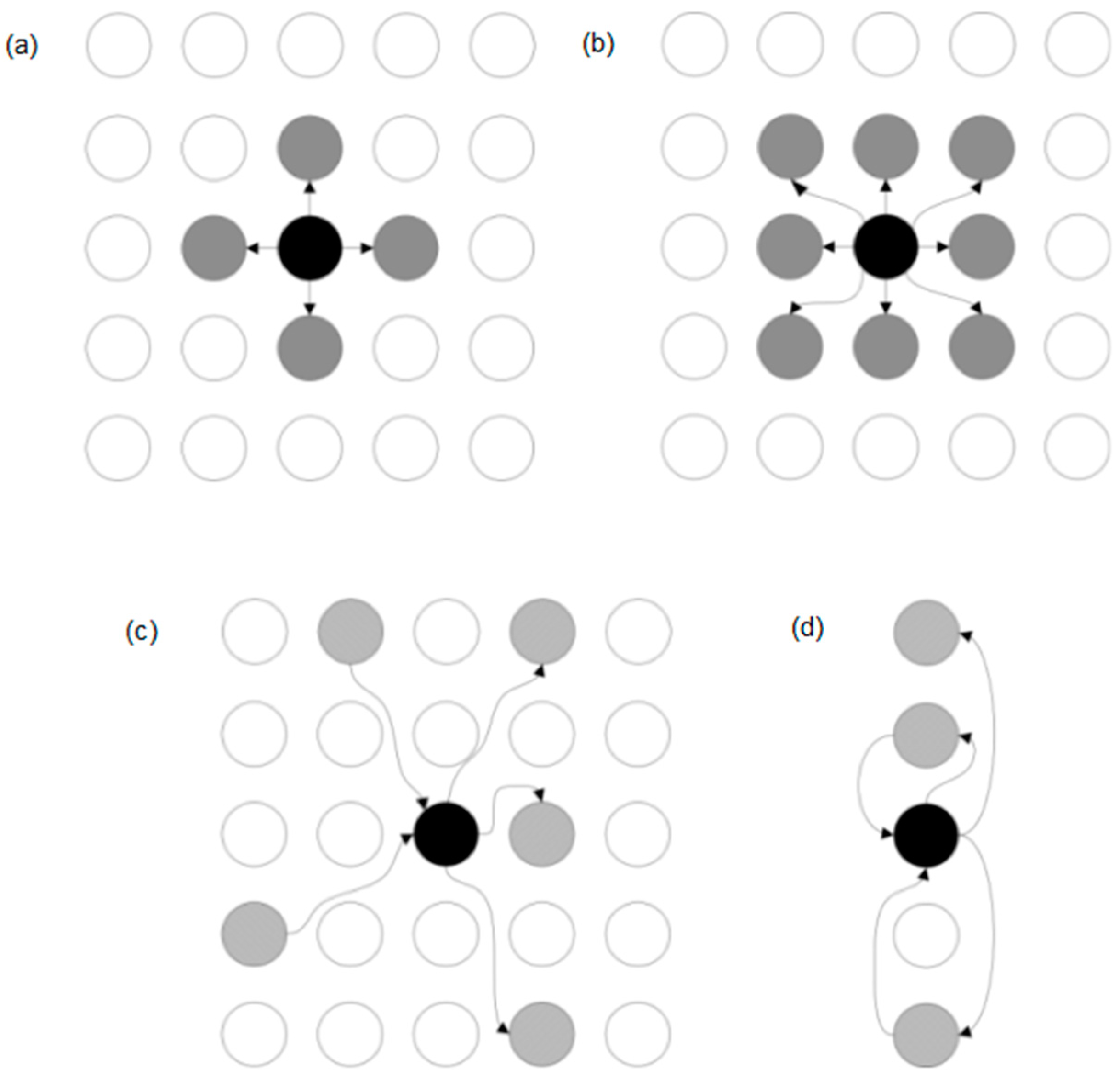
A sample interpretation of mutual relation-based connections is presented in Figure 16. The presentation ignores the weights of the arcs, which may correspond to the relations defined in a specific r–GCA automaton.
The analysis of the obtained graphs shows that realistic traffic simulation is an asymmetrical phenomenon. Symmetry in the graph is visible only in some special cases, when the graph represents the traffic determined in time (not changing) and when there is a very small number of vehicles on the road.
The use of r–GCA removes the limitations of classical CA associated with the modeling of spatially distributed objects (having a fixed number of neighbours arranged in regular neighbourhoods, on which the state of the currently considered cell depends). The proposed machine enables modeling in the relational and logical space—where the neighbourhood corresponds to the relationships in the considered model.
Therefore, r–GCA should be considered as a mechanism that enables us to obtain a different level of realism in modelling phenomena in the real world compared to classical CA.
Further works in this regard will be focused on modelling of phenomena that are relation-based, both in the real and virtual world. Additionally, the works will involve the hardware side supporting the computations.
6. Conclusions
The graph cellular automaton (r–GCA) proposed in this article enables the modelling of complex systems, defined as a set of interacting objects (the system elements). If objects are of the same type (homogeneous), and the system structure specifies the relations between them, such a system seems to be appropriate for modelling, with the use of the proposed automaton.
Compared to classical automata, where cells usually correspond to objects neighbouring in the d-dimension space (e.g., adjacent land plots, elements of a two-dimensional grid representing surface area, and three-dimensional grid representing volume), r–GCA enable modelling the following phenomena:
- In d-dimensional space (if the neighbourhood specified by a graph is defined in such a way so as to correspond to the neighbourhood in classical CA, e.g., Moore’s or von Neumann’s neighbourhood);
- In virtual or relation-based space—where neighbourhood does not correspond to the relation of the cells location in the space, but it is relation-based.
In order to demonstrate the usefulness of the developed automaton, the first study of this kind was performed to compare the classical traffic model to a graph cellular automaton adapted to simulate road traffic. It was shown that the developed model enabled comparable modelling and simulation of road traffic. However, the graph structures proved to be more demanding in terms of processor operation time. Nevertheless, taking into account the progressive development of computer hardware and compilers that optimize the code, as well as the rules that parallelise the computations, the extended processor operation time may be substantially shortened in the next implementations.
Acknowledgments
I would like to express my particular appreciation to Grzegorz Hołowiński for his professional support in the area of graph structures, and to Artur Kos for his invaluable help regarding the software for the developed model.
Conflicts of Interest
The author declares no conflict of interest.
References
- Wolfram, S. A New Kind of Science; Wolfram Media: Champaign, IL, USA, 2002. [Google Scholar]
- Ilachinsky, A.; Halpern, P. Structurally Dynamic Cellular Automata. Complex Syst. 1987, 1, 503–527. [Google Scholar]
- Alonso-Sanz, R. A Structurally Dynamic Cellular Automaton with Memory in the Triangular Tessellation. Complex Syst. 2007, 17, 1–15. [Google Scholar]
- Bersini, H.; Detours, V. Asynchrony induces stability in cellular automata based models. In Artificial Life IV: Proceedings of the Fourth International Workshop on the Synthesis and Simlulation of Living Systmes, Cambridge, MA, USA; MIT Press: Cambridge, MA, USA, 1994; pp. 382–387. [Google Scholar]
- Cornforth, D.; Green, D.G.; Newth, D.; Kirley, M. Do Artificial Ants March in Step? Ordered Asynchronous Processes and Modularity, Biological Systems. In Proceedings of the 18th International Conference on Artificial Life, Sydney, Australia, 9–13 December 2002; Standish, B., Abbass, A., Eds.; pp. 28–32. [Google Scholar]
- Couclelis, H. From cellular automata to urban models: New principles for model development and implementation. Environ. Plan. B Plan. Des. 1997, 24, 165–174. [Google Scholar] [CrossRef]
- Takeyama, M.; Couclelis, H. Map dynamics: Integrating cellular automata and GIS through Geo–Algebra. Int. J. Geogr. Inf. Sci. 1997, 11, 73–91. [Google Scholar] [CrossRef]
- O’Sullivan, D. Graph-cellular automata: A generalised discrete urban and regional model. Environ. Plan. B Plan. Des. 2001, 28, 687–705. [Google Scholar] [CrossRef]
- Neumann, J.V. Theory of Self-Reproducing Automata; University of Illinois Press: Champaign, IL, USA, 1966. [Google Scholar]
- Wolfram, S. Computation theory of cellular automata. Commun. Math. Phys. 1984, 96, 15–57. [Google Scholar] [CrossRef]
- Wolfram, S. Universality and complexity in cellular automata. Physica D 1984, 10, 1–35. [Google Scholar] [CrossRef]
- Gutowitz, H. Cellular automata and the sciences of complexity, part I. Complexity 1996, 1, 16–22. [Google Scholar] [CrossRef]
- Gutowitz, H. Cellular automata and the sciences of complexity, part II. Complexity 1996, 1, 29–35. [Google Scholar] [CrossRef]
- Nandi, S.; Kar, B.K.; Chaudhuri, P.P. Theory and applications of cellular automata in cryptography. IEEE Trans. Comput. 1994, 43, 1346–1357. [Google Scholar] [CrossRef]
- Seredynski, F.; Bouvry, P.; Zomaya, A.Y. Cellular automata computations and secret key cryptography. Parallel Comput. 2004, 30, 753–766. [Google Scholar] [CrossRef]
- Georgoudas, I.; Sirakoulis, G.C.; Scordilis, E.; Andreadis, I. A cellular automaton simulation tool for modelling seismicity in the region of Xanthi. Environ. Model. Softw. 2007, 22, 1455–1464. [Google Scholar] [CrossRef]
- Petrica, L. FPGA Optimized Cellular Automaton Random Number Generator. J. Parallel Distrib. Comput. 2017, 111, 251–259. [Google Scholar] [CrossRef]
- Toffoli, T.; Margolus, N. Cellular Automata Machines: A New Environment for Modeling; MIT Press: Cambridge, MA, USA, 1987. [Google Scholar]
- Wuensche, A. Classifying cellular automata automatically. Complexity 1999, 4, 47–66. [Google Scholar] [CrossRef]
- Sutner, K. Classification of cellular automata. Encycl. Complex. Syst. Sci. 2009, 3, 755–768. [Google Scholar]
- Gilman, R.H. Classes of linear automata. Ergod. Theory Dyn. Syst. 1987, 7, 105–118. [Google Scholar] [CrossRef]
- Cattaneo, G.; Formenti, E.; Margara, L. Topological definitions of deterministic chaos. In Cellular Automata; Springer: Dordrecht, The Netherlands, 1999; pp. 213–259. [Google Scholar]
- Javid, M.A.J.; Alghamdi, W.; Ursyn, A.; Zimmer, R.; al-Rifaie, M.M. Swarmic approach for symmetry detection of cellular automata behaviour. Soft Comput. 2017, 21, 5585–5599. [Google Scholar] [CrossRef]
- Hoffmann, R.; Völkmann, K.P.; Waldschmidt, S. GCA: Global Cellular Automata GCA. A Flexible Parallel Model. In International Conference on Parallel Computing Technologies; Springer: London, UK, 2001; pp. 66–73. [Google Scholar]
- Barredo, J.I.; Kasanko, M.; McCormick, N.; Lavalle, C. Modelling dynamic spatial processes: Simulation of urban future scenarios through cellular automata. Landsc. Urban Plan. 2003, 64, 145–160. [Google Scholar] [CrossRef]
- Stevens, D.; Dragićević, S. A GIS-based irregular cellular automata model of land-use change. Environ. Plan. B Plan. Des. 2007, 34, 708–724. [Google Scholar] [CrossRef]
- Santé, I.; García, A.M.; Miranda, D.; Crecente, R. Cellular automata models for the simulation of real-world urban processes: A review and analysis. Landsc. Urban Plan. 2010, 96, 108–122. [Google Scholar] [CrossRef]
- Triantakonstantis, D.; Mountrakis, G. Urban growth prediction: A review of computational models and human perceptions. J. Geogr. Inf. Syst. 2012, 4, 555–587. [Google Scholar] [CrossRef]
- Barreira-González, P.; Barros, J. Configuring the neighbourhood effect in irregular cellular automata based models. Int. J. Geogr. Inf. Sci. 2017, 31, 617–636. [Google Scholar] [CrossRef]
- Dahal, K.R.; Chow, T.E. Characterization of neighborhood sensitivity of an irregular cellular automata model of urban growth. Int. J. Geogr. Inf. Sci. 2015, 29, 475–497. [Google Scholar] [CrossRef]
- Barreira-González, P.; Gómez-Delgado, M.; Aguilera-Benavente, F. From raster to vector cellular automata models: A new approach to simulate urban growth with the help of graph theory. Comput. Environ. Urban Syst. 2015, 54, 119–131. [Google Scholar] [CrossRef]
- Róka, Z. One-way cellular automata on Cayley graphs. Theor. Comput. Sci. 1994, 132, 259–290. [Google Scholar] [CrossRef]
- Marr, C.; Hütt, M.T. Topology regulates pattern formation capacity of binary cellular automata on graphs. Phys. A Stat. Mech. Appl. 2005, 354, 641–662. [Google Scholar] [CrossRef]
- Rinaldi, P.; Dalponte, D.; Vénere, M.; Clausse, A. Graph-based cellular automata for simulation of surface flows in large plains. Asian J. Appl. Sci. 2012, 5, 224–231. [Google Scholar]
- Rinaldi, P.R.; Dalponte, D.D.; Vénere, M.J.; Clausse, A. Cellular automata algorithm for simulation of surface flows in large plains. Simul. Model. Pract. Theory 2007, 15, 315–327. [Google Scholar] [CrossRef]
- Liao, M.J.; Wang, K.Y.; Meng, X.Q. Simulation of ticket hall queuing behavior in transit station based on cellular automata model. In Proceedings of the 2010 International Conference on E-Product E-Service and E-Entertainment (ICEEE), Henan, China, 7–9 November 2010; pp. 1–4. [Google Scholar]
- Martínez, M.J.F.; Merino, E.G.; Sánchez, E.G.; Sánchez, J.E.G.; del Rey, A.M.; Sánchez, G.R. A graph cellular automata model to study the spreading of an infectious disease. In Mexican International Conference on Artificial Intelligence; Springer: Berlin/Heidelberg, Germany, 2012; pp. 458–468. [Google Scholar]
- Leporati, A.; Mariot, L. 1-Resiliency of bipermutive cellular automata rules. In International Workshop on Cellular Automata and Discrete Complex Systems; Springer: Berlin/Heidelberg, Germany, 2013; pp. 110–123. [Google Scholar]
- Sethi, B.; Das, S. Modeling of asynchronous cellular automata with fixed-point attractors for pattern classification. In Proceedings of the 2013 International Conference on High Performance Computing and Simulation (HPCS), Helsinki, Finland, 1–5 July 2013; pp. 311–317. [Google Scholar]
- Marr, C.; Hütt, M.T. Cellular automata on graphs: Topological properties of ER graphs evolved towards low-entropy dynamics. Entropy 2012, 14, 993–1010. [Google Scholar] [CrossRef]
- Tretyakova, A.; Seredynski, F.; Bouvry, P. Graph Cellular Automata approach to the Maximum Lifetime Coverage Problem in wireless sensor networks. Simulation 2016, 92, 153–164. [Google Scholar] [CrossRef]
- Małecki, K.; Jankowski, J.; Rokita, M. Application of Graph Cellular Automata in Social Network Based Recommender System. In International Conference on Computational Collective Intelligence; Springer: Berlin/Heidelberg, Germany, 2013; pp. 21–29. [Google Scholar]
- Weimar, J.R. Cellular automata for reaction-diffusion systems. Parallel Comput. 1997, 23, 1699–1715. [Google Scholar] [CrossRef]
- West, D.B. Introduction to Graph Theory; Prentice Hall: Upper Saddle River, NJ, USA, 2001; Volume 2. [Google Scholar]
- Nagel, K.; Schreckenberg, M. A cellular automaton model for freeway traffic. J. Phys. I 1992, 2, 2221–2229. [Google Scholar] [CrossRef]
- Hoogendoorn, S.; Bovy, P. State-of-the-art of vehicular traffic flow modelling. Proc. Inst. Mech. Eng. Part I J. Syst. Control Eng. 2001, 215, 283–303. [Google Scholar] [CrossRef]
- Biham, O.; Middleton, A.A.; Levine, D. Self-organization and a dynamical transition in traffic-flow models. Phys. Rev. A 1992, 46, R6124–R6127. [Google Scholar] [CrossRef] [PubMed]
- Schadschneider, A.; Schreckenberg, M. Traffic flow models with ‘slow-to-start’rules. Ann. Phys. 1997, 509, 541–551. [Google Scholar] [CrossRef]
- Chopard, B.; Luthi, P.O.; Queloz, P. Cellular automata model of car traffic in a two-dimensional street network. J. Phys. A 1996, 29, 2325–2336. [Google Scholar] [CrossRef]
- Jost, D.; Nagel, K. Probabilistic Traffic Flow Breakdown in Stochastic Car Following Models. In Proceedings of the Transportation Research Board 82nd Annual Meeting compendium of papers CD-ROM, Washington, DC, USA, 12–16 January 2003; pp. 3–42. [Google Scholar]
- Fukui, M.; Ishibashi, Y. Traffic flow in 1D cellular automaton model including cars moving with high speed. J. Phys. Soc. Jpn. 1996, 65, 1868–1870. [Google Scholar] [CrossRef]
- Nagel, K.; Wolf, D.E.; Wagner, P.; Simon, P. Two-lane traffic rules for cellular automata: A systematic approach. Phys. Rev. E 1998, 58, 1425–1437. [Google Scholar] [CrossRef]
- Lan, L.; Chang, C.W. Inhomogeneous cellular automata modeling for mixed traffic with cars and motorcycles. J. Adv. Transp. 2005, 39, 323–349. [Google Scholar] [CrossRef]
- Vasic, J.; Ruskin, H.J. Cellular automata simulation of traffic including cars and bicycles. Phys. A Stat. Mech. Appl. 2012, 391, 2720–2729. [Google Scholar] [CrossRef]
- Rickert, M.; Nagel, K.; Schreckenberg, M.; Latour, A. Two lane traffic simulations using cellular automata. Phys. A Stat. Mech. Appl. 1996, 231, 534–550. [Google Scholar] [CrossRef]
- Chowdhury, D.; Wolf, D.E. Praticle hopping models for two-lane traffic with two kinds of vehicles: Effects of lane-changing rules. Phys. A Stat. Mech. Appl. 1997, 235, 417–439. [Google Scholar] [CrossRef]
- Knospe, W.; Santen, L.; Schadschneider, A.; Schreckenberg, M. Disorder effects in cellular automata for two-lane traffic. Phys. A Stat. Mech. Appl. 1999, 265, 614–633. [Google Scholar] [CrossRef]
- Wang, Y.M.; Zhou, L.S.; Lv, Y.B. Cellular automaton traffic flow model considering flexible safe space for lane-changing. J. Syst. Simul. 2008, 20, 1159–1162. [Google Scholar]
- Wang, Y.M. Studies on Traffic Organization Planning and Traffic Flow Simulation under the Influence of Major Public Emergencies; Beijing Jiaotong University: Beijing, China, 2009. [Google Scholar]
- Xu, H.X.; Zhang, D.M. A cellular automaton model based on improved rules of flexible safe lane-changing distance. J. Shenyang Univ. (Nat. Sci. Ed.) 2014, 26, 369–371. [Google Scholar]
- Xu, H.; Xu, M. A cellular automata traffic flow model based on safe lane-changing distance constraint rule. In Proceedings of the 2016 IEEE Advanced Information Management, Communicates, Electronic and Automation Control Conference (IMCEC), Xi’an, China, 3–5 October 2016; pp. 1253–1256. [Google Scholar]
- Daganzo, C. In traffic flow, cellular automata = kinematic waves. Transp. Res. Part B 2006, 40, 396–403. [Google Scholar] [CrossRef]
- Wang, R.; Liu, M. A realistic cellular automata model to simulate traffic flow at urban roundabouts. In International Conference on Computational Science; Springer: Berlin/Heidelberg, Germany, 2005; Volume 3515, pp. 420–427. [Google Scholar]
- Feng, Y.; Liu, Y.; Deo, P.; Ruskin, H.J. Heterogeneous Traffic Flow Model for a Two-Lane Roundabout and Controlled Intersection. Int. J. Mod. Phys. C 2007, 18, 107–117. [Google Scholar] [CrossRef]
- Małecki, K.; Wątróbski, J. Cellular Automaton to Study the Impact of Changes in Traffic Rules in a Roundabout: A Preliminary Approach. Appl. Sci. 2017, 7, 742. [Google Scholar] [CrossRef]
- Liu, M.Z.; Zhao, S.B.; Wang, R.L. A cellular automaton model for heterogeneous and incosistent driver behavior in urban traffic. Commun. Theor. Phys. 2012, 58, 744–748. [Google Scholar] [CrossRef]
- Małecki, K.; Iwan, S. Development of Cellular Automata for Simulation of the Crossroads Model with a Traffic Detection System. In International Conference on Transport Systems Telematics; Springer: Berlin/Heidelberg, Germany, 2012; Volume 329, pp. 276–283. [Google Scholar]
- Heeroo, K.N.; Gukhool, O.; Hoorpah, D. A Ludo Cellular Automata model for microscopic traffic flow. J. Comput. Sci. 2016, 16, 114–127. [Google Scholar] [CrossRef]
- Małecki, K. The Use of Heterogeneous Cellular Automata to Study the Capacity of the Roundabout. In International Conference on Artificial Intelligence and Soft Computing; Springer: Cham, Switzerland, 2017; pp. 308–317. [Google Scholar]
- Iwan, S.; Małecki, K. Utilization of cellular automata for analysis of the efficiency of urban freight transport measures based on loading/unloading bays example. Transp. Res. Procedia 2017, 25, 1021–1035. [Google Scholar] [CrossRef]
- Iwan, S.; Kijewska, K.; Johansen, B.G.; Eidhammer, O.; Małecki, K.; Konicki, W.; Thompson, R.G. Analysis of the environmental impacts of unloading bays based on cellular automata simulation. Transp. Res. D Transp. Environ. 2017. [Google Scholar] [CrossRef]
Figure 1.
Changing the graph structure: (a) exemplary graph; (b) after vertex removal; (c) after edge removal; (d) after vertex addition; (e) after edge addition.
Figure 1.
Changing the graph structure: (a) exemplary graph; (b) after vertex removal; (c) after edge removal; (d) after vertex addition; (e) after edge addition.

Figure 2.
An example of a graph describing the relational neighbourhood of objects in a modeled system. The vertices of the graph correspond to the cells of cellular automata (CA).
Figure 2.
An example of a graph describing the relational neighbourhood of objects in a modeled system. The vertices of the graph correspond to the cells of cellular automata (CA).

Figure 3.
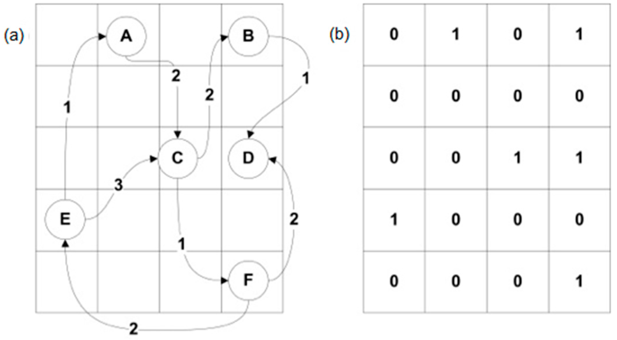
Objects and corresponding relations mapped to cells of r–GCA: (a) relation based neighbourhood graph and (b) corresponding activity matrix of CA cells (1: activated cell, 0: deactivated cell).
Figure 3.
Objects and corresponding relations mapped to cells of r–GCA: (a) relation based neighbourhood graph and (b) corresponding activity matrix of CA cells (1: activated cell, 0: deactivated cell).

Figure 4.
Graph and neighbourhood matrix.
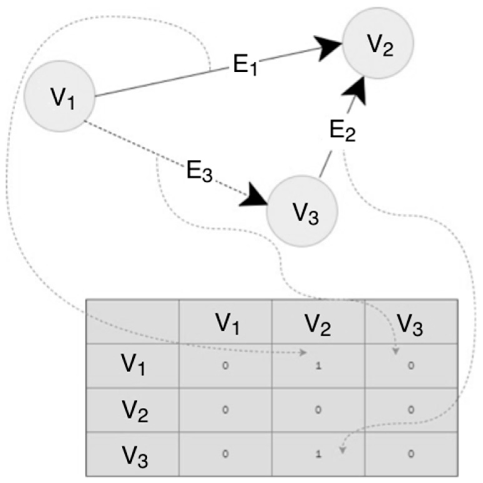
Figure 5.
A fragment of a two-way road with sample vehicles.

Figure 6.
A graph made as per the situation in Figure 5.
Figure 6.
A graph made as per the situation in Figure 5.
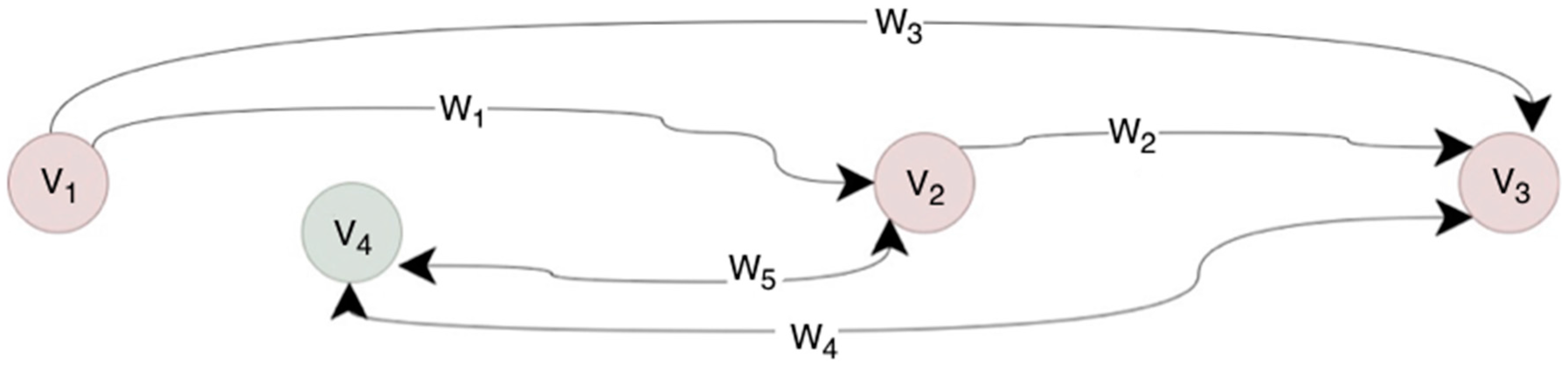
Figure 7.
Neighbourhood matrix—.

Figure 8.
Matrix of weights—.

Figure 9.
Overtaking stage—the analysis of weights.
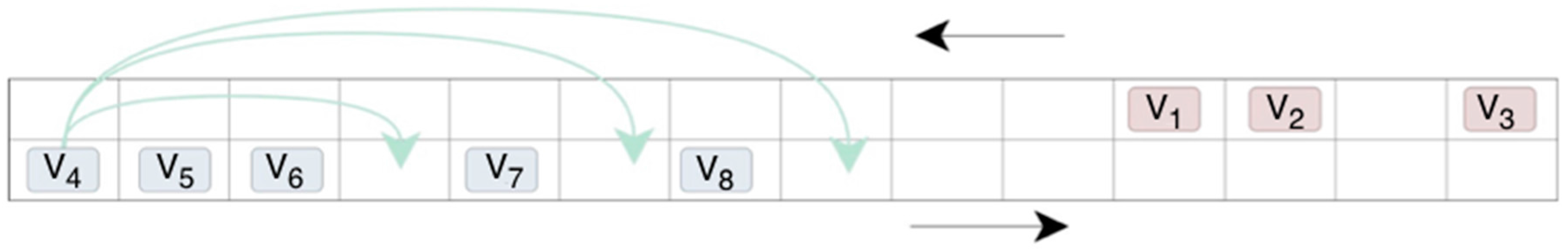
Figure 10.
Constituents of the operation time of a single iteration in the simulation process.

Figure 11.
Comparison of mean minimum speeds of moving vehicles.
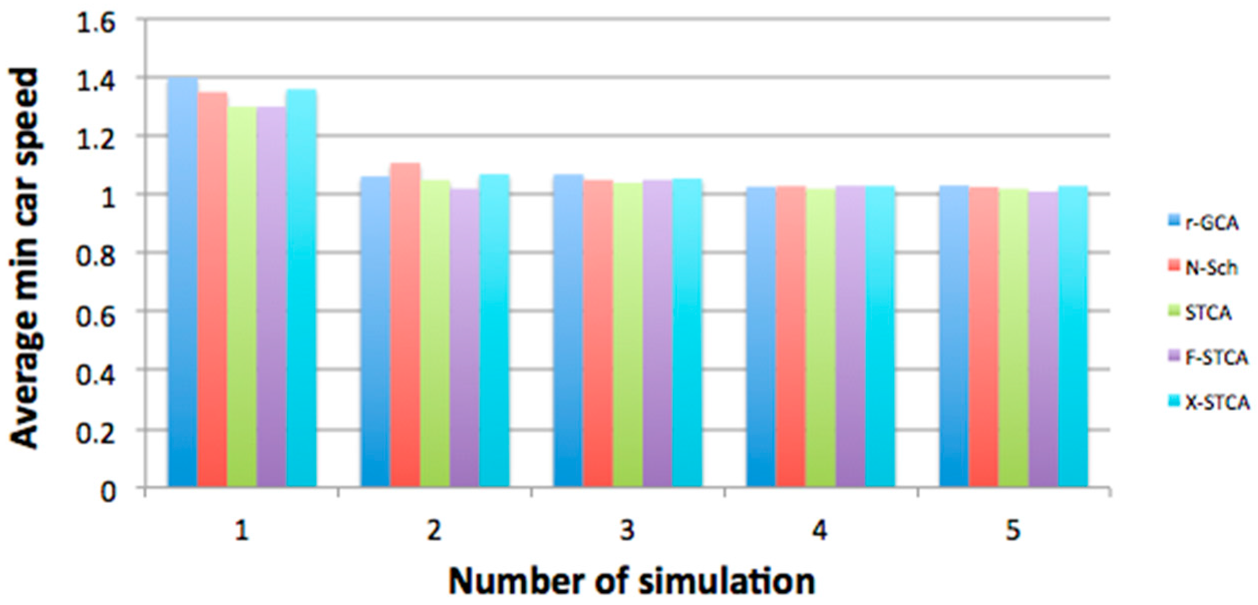
Figure 12.
Comparison of mean maximum speeds of moving vehicles.
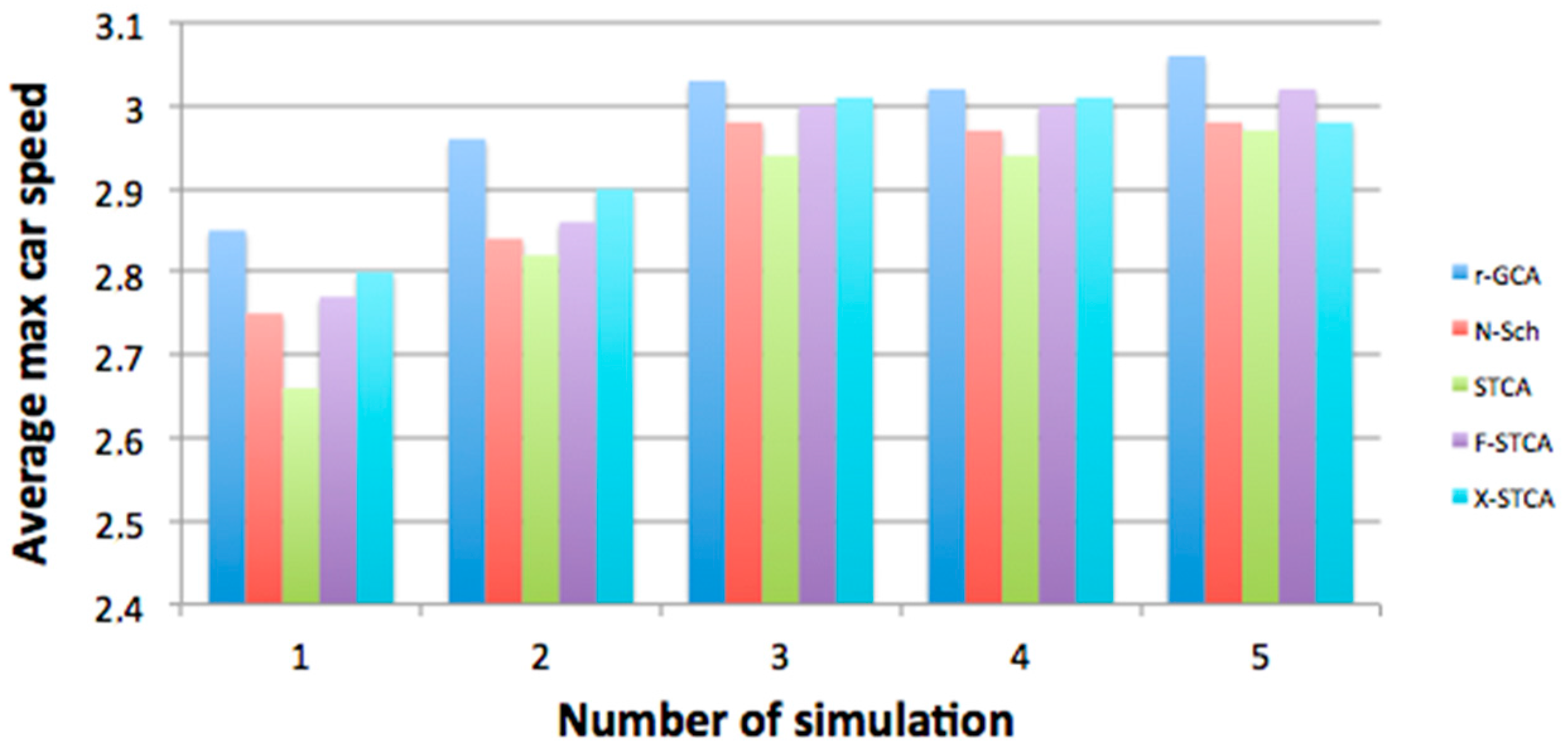
Figure 13.
Comparing the total simulation time.

Figure 14.
A map of the analysed road.
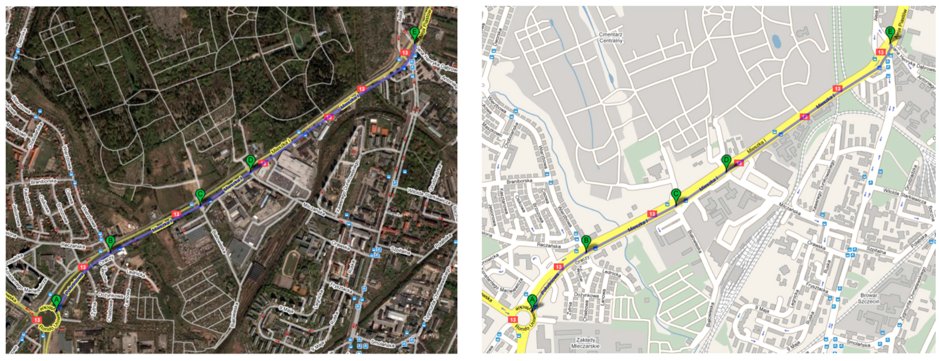
Figure 15.
Average number of vehicles for different speed limits.
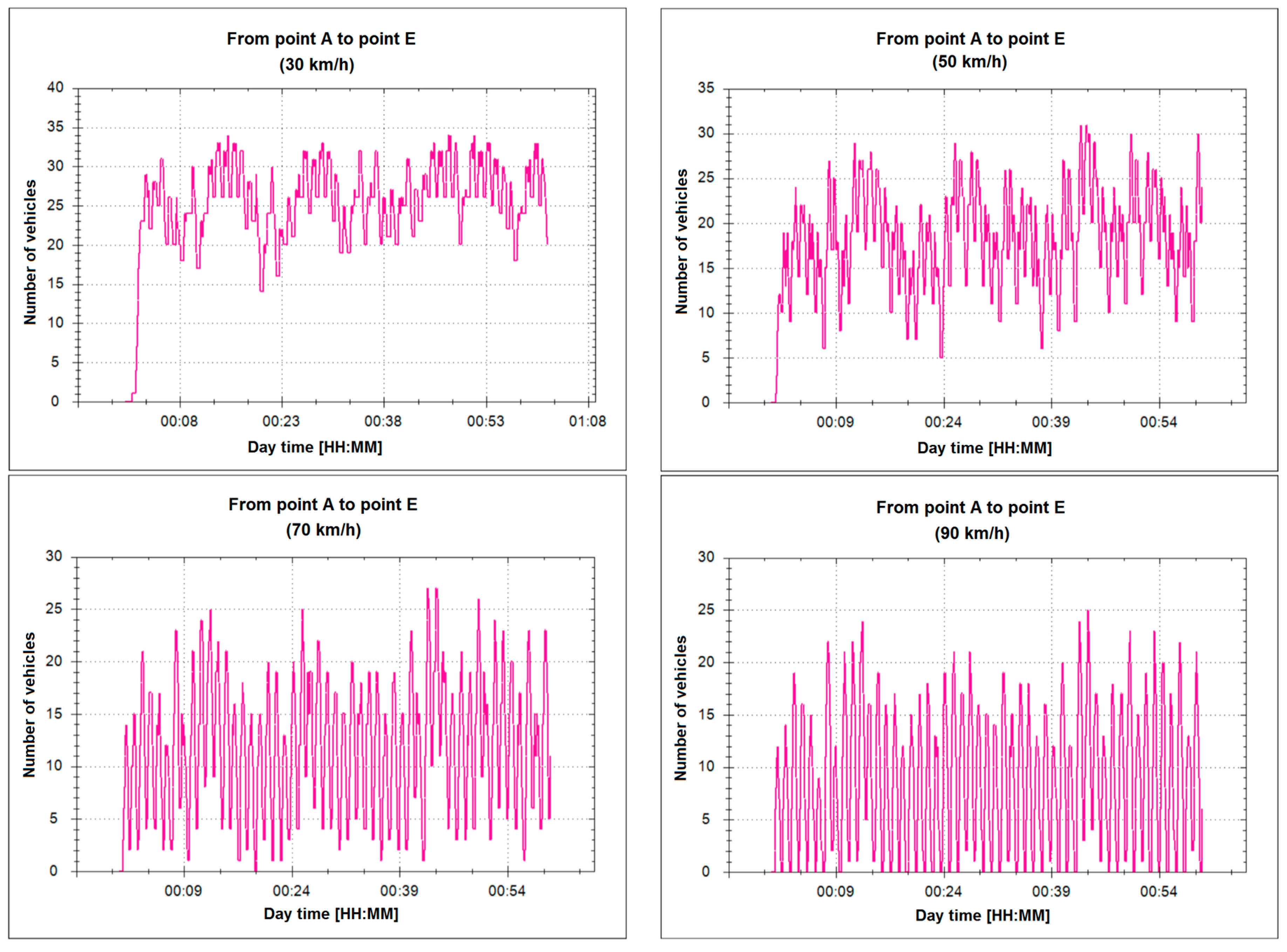
Figure 16.
Types of neighbourhoods in a graph cellular automaton (relation-based graph cellular automation (r–GCA)): analogous to Moore’s (a) or von Neumann’s neighbourhood (b) in a classical CA; in r–GCA independent from the distance in the d-dimensional space of the cells (c,d).
Figure 16.
Types of neighbourhoods in a graph cellular automaton (relation-based graph cellular automation (r–GCA)): analogous to Moore’s (a) or von Neumann’s neighbourhood (b) in a classical CA; in r–GCA independent from the distance in the d-dimensional space of the cells (c,d).


Table 1.
A comparison of cellular automata of different types.
| Characteristic | Cellular Automata | |||
|---|---|---|---|---|
| Homogeneous CA | Structurally Dynamic CA [2,3] | Asynchronous CA [4,5] | Graph CA [8] | |
| Grid of cells | In d-dimensional space (d ≥ 1) | 2–dimensional space | In d-dimensional space (d ≥ 1), 2-dimensional | Irregular structure, in 2-dimensional space |
| State of automaton | Depends on states of all cells | Depends on states of all cells | Depends on states of all cells | Depends on states of all cells |
| Set of states for each cell | Identical | Identical | Identical | Identical |
| Change of state of cells | Synchronous | Synchronous | Asynchronous | Synchronous |
| Grid of automaton | Unchanging over time | Unchanging over time | Unchanging over time | Unchanging over time |
| Neighbourhood diagram for entire grid | Regular | Quasi-regular. Neighbourhood described by a set of neighbourhoods | Regular | Neighbourhoods described by a graph |
| Rule complexity | Elementary | Elementary | Elementary | Elementary or complex (depending on automaton) |
| Combining with automata of the same type | Impossible | Impossible | Impossible | Possible as a hierarchical graph combination. |
Table 2.
Simulation results for the road presented in Figure 15.
Table 2.
Simulation results for the road presented in Figure 15.
| Speed [km/h] | Number of Vehicles | Time [M:SS] |
|---|---|---|
| 30 | 1065 | 5:48 |
| 50 | 1087 | 3:56 |
| 70 | 1114 | 2:47 |
| 90 | 1128 | 2:13 |
© 2017 by the author. Licensee MDPI, Basel, Switzerland. This article is an open access article distributed under the terms and conditions of the Creative Commons Attribution (CC BY) license (http://creativecommons.org/licenses/by/4.0/).
Share and Cite
MDPI and ACS Style
Małecki, K. Graph Cellular Automata with Relation-Based Neighbourhoods of Cells for Complex Systems Modelling: A Case of Traffic Simulation. Symmetry 2017, 9, 322. https://doi.org/10.3390/sym9120322
AMA Style
Małecki K. Graph Cellular Automata with Relation-Based Neighbourhoods of Cells for Complex Systems Modelling: A Case of Traffic Simulation. Symmetry. 2017; 9(12):322. https://doi.org/10.3390/sym9120322
Chicago/Turabian StyleMałecki, Krzysztof. 2017. "Graph Cellular Automata with Relation-Based Neighbourhoods of Cells for Complex Systems Modelling: A Case of Traffic Simulation" Symmetry 9, no. 12: 322. https://doi.org/10.3390/sym9120322
Note that from the first issue of 2016, this journal uses article numbers instead of page numbers. See further details here.