Cyclotomic Aperiodic Substitution Tilings

Abstract

The class of Cyclotomic Aperiodic Substitution Tilings (CASTs) is introduced. Its vertices are supported on the $2n$-th cyclotomic field. It covers a wide range of known aperiodic substitution tilings of the plane with finite rotations. Substitution matrices and minimal inflation multipliers of CASTs are discussed as well as practical use cases to identify specimen with individual dihedral symmetry $D_n$ or $D_{2n}$, i.e., the tiling contains an infinite number of patches of any size with dihedral symmetry $D_n$ or $D_{2n}$ only by iteration of substitution rules on a single tile.

1. Introduction

Tilings have been the subject of wide research. Many of their properties are investigated and discussed in view of their application in physics and chemistry, e.g., in detail in the research of crystals and quasicrystals, such as D. Shechtman et al.’s renowned Al-Mn-alloy with icosahedral point group symmetry [1]. Tilings are also of mathematical interest on their own [2,3].

Without any doubt, they have great aesthetic qualities as well. Some of the most impressive examples are the tilings in M. C. Escher’s art works [4], H. Voderberg’s spiral tiling [5,6] and the pentagonal tilings of A. Dürer, J. Kepler and R. Penrose [2,7], just to name a few.

In contrast to a scientist, a designer may have different requirements. Nevertheless the result may have interesting mathematical properties. Due to the lack of a general criteria for subjective matters of taste, we consider the following properties as preferable:

• The tiling shall be aperiodic and repetitive (locally indistinguishable) to have an interesting (psychedelic) appearance.
• The tiling shall have a small inflation multiplier for reasons of economy. Large inflation multipliers either require large areas to be covered or many tiles of a small size to be used.
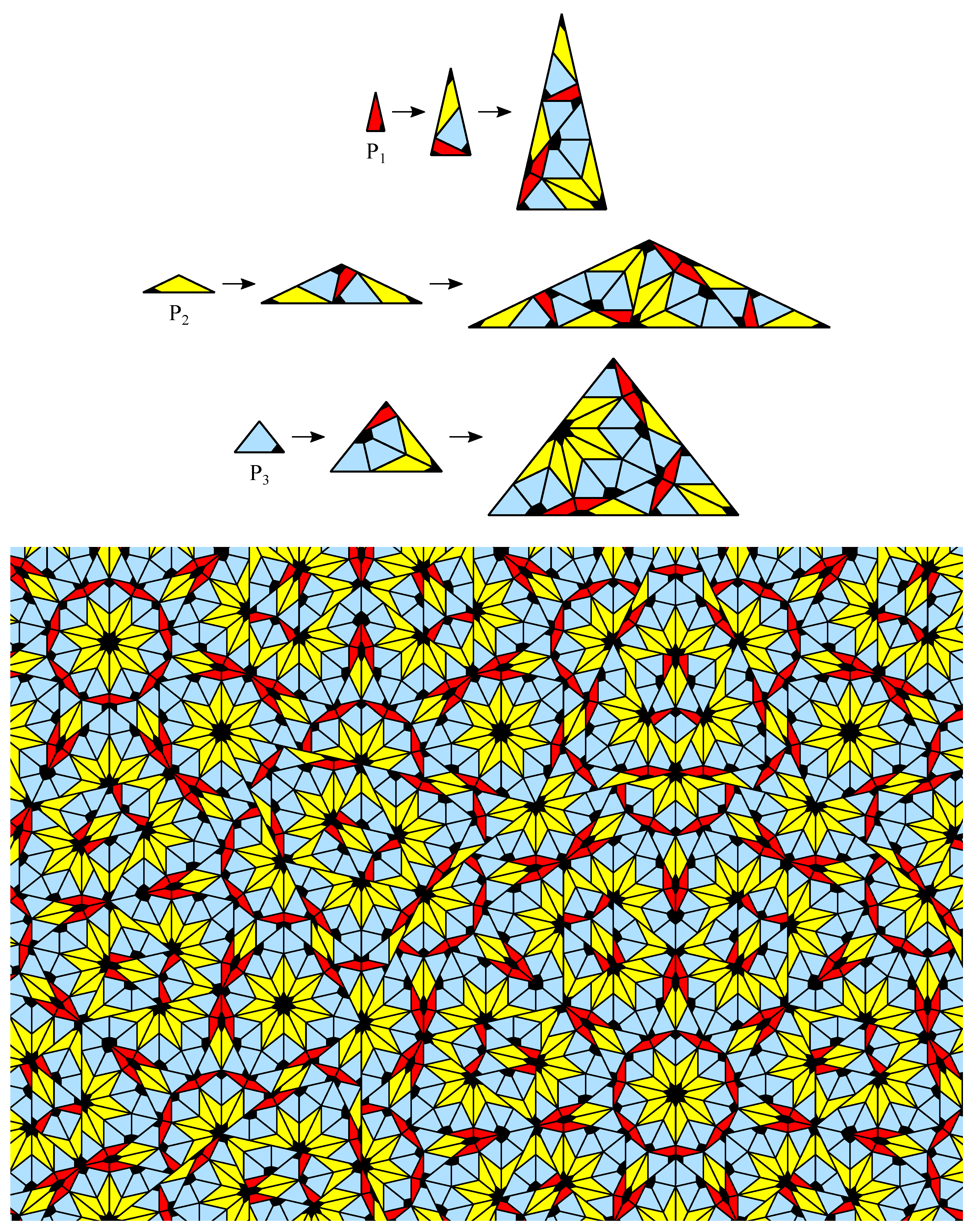
• The tiling shall yield “individual dihedral symmetry” $D_n$ or $D_{2n}$ with $n\ge 4$. In other words, it shall contain an infinite number of patches of any size with dihedral symmetry only by iteration of substitution rules on a single tile.
  Similar to G. Maloney we demand symmetry of individual tilings and not only symmetry of tiling spaces [8].

The most common methods to generate aperiodic tilings are:

• Matching rules, as introduced in the very first publication of an aperiodic tiling, the Wang-tiling by R. Berger [9]. See [10,11,12] for more details.
• Cut-and-project scheme, first described by de Bruijn for the Penrose tiling in [13], later extended to a general method, see [14,15] and references therein for more details, notably the earlier general method described in [16].
• Duals of multi grids as introduced by de Bruijn [17] with equidistant spacings are equivalent to the cut-and-project scheme [18].
  Duals of multi grids with aperiodic spacings as introduced by Ingalls [19,20] are close related to Ammann bars, see [2,10,21] and [22] (Chapter 5) for details and examples.
• The idea of substitution rules or substitutions in general is a rather old concept, e.g., Koch’s snowflake [23,24,25] or Rep-Tilings [26]. However, it seems its first consequent application to tile the whole Euclidean plane aperiodically appeared with the Penrose tiling [2,3,27,28,29].

Among those methods, substitution rules may be the easiest approach to construct aperiodic tilings. Additionally, they have some other advantages:

• The inflation multipliers of tilings obtained by the cut-and-project scheme are limited to PV-numbers. According to [14,15] this was first noted by [16]. This limitation does not apply to substitution tilings.
• Matching rules tend to be more complex than substitution rules. See [30,31] for examples.

In view of the preferable properties we will introduce the class of Cyclotomic Aperiodic Substitution Tilings (CAST). Its vertices are supported on the $2n$-th cyclotomic field. It covers a wide range of known aperiodic substitution tilings of the plane with finite rotations. Its properties, in detail: substitution matrices, minimal inflation multiplier and aperiodicity, are discussed in Section 2. CASTs with minimal or at least small inflation multiplier are presented in Section 3 and Section 4, which also includes a generalization of the Lançon-Billard tiling. Section 5 focuses on several cases of rhombic CASTs and their minimal inflation multiplier. In Section 6 the “Gaps to Prototiles” algorithm is introduced, which allows to identify large numbers of new CASTs. Finally, examples of Girih CASTs with $n\in \left\{4,5,7\right\}$ are presented in Section 7. Except the generalized Lançon-Billard tiling all CASTs in this article yield local dihedral symmetry $D_n$ or $D_{2n}$.

For terms and definitions we stay close to [3,32]:

• A “tile” in ${\mathbb{R}}^d$ is defined as a nonempty compact subset of ${\mathbb{R}}^d$ which is the closure of its interior.
• A “tiling” in ${\mathbb{R}}^d$ is a countable set of tiles, which is a covering as well as a packing of ${\mathbb{R}}^d$. The union of all tiles is ${\mathbb{R}}^d$. The intersection of the interior of two different tiles is empty.
• A “patch” is a finite subset of a tiling.
• A tiling is called “aperiodic” if no translation maps the tiling to itself.
• “Prototiles” serve as building blocks for a tiling.
• Within this article the term “substitution” means, that a tile is expanded with a linear map—the “inflation multiplier”—and dissected into copies of prototiles in original size—the “substitution rule”.
• A “supertile” is the result of one or more substitutions, applied to a single tile. Within this article we use the term for one substitutions only.
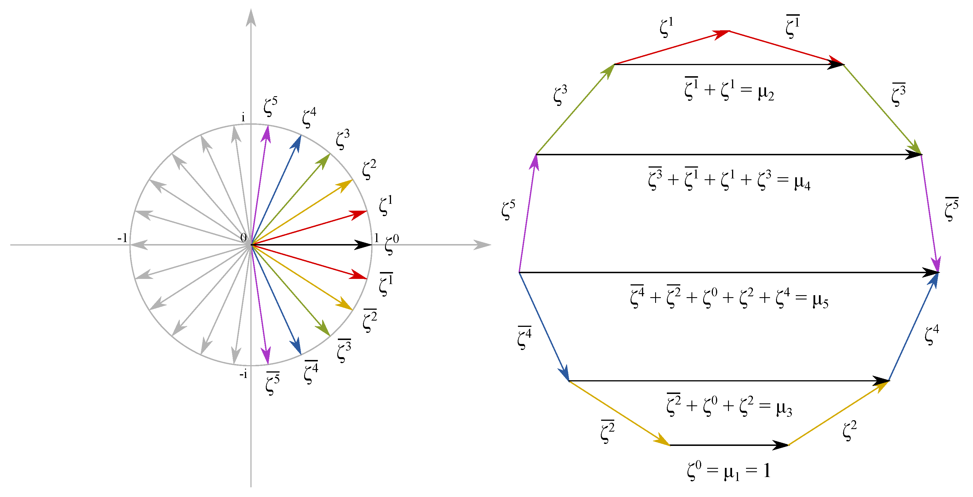
• We use ${\zeta }_n^k$ to denote the n-th roots of unity so that ${\zeta }_n^k=e^{\frac{2\mathtt{i}k\pi }{n}}$and its complex conjugate $\overline{{\zeta }_n^k}=e^{-\frac{2\mathtt{i}k\pi }{n}}$.
• $\mathbb{Q}\left({\zeta }_n\right)$ denotes the n-th cyclotomic field. Please note that $\mathbb{Q}\left({\zeta }_n\right)=\mathbb{Q}\left({\zeta }_{2n}\right)$ for $oddn$.
• The maximal real subfield of $\mathbb{Q}\left({\zeta }_n\right)$ is $\mathbb{Q}\left({\zeta }_n+\overline{{\zeta }_n}\right)$.
• $\mathbb{Z}\left[{\zeta }_n\right]$ denotes the the ring of algebraic integers in $\mathbb{Q}\left({\zeta }_n\right)$.
• $\mathbb{Z}\left[{\zeta }_n+\overline{{\zeta }_n}\right]$ denotes the the ring of algebraic integers (which are real numbers) in $\mathbb{Q}\left({\zeta }_n+\overline{{\zeta }_n}\right)$.
• We use ${\mu }_{n,k}$ to denote the k-th diagonal of a regular n-gon with side length ${\mu }_{n,1}={\mu }_{n,n-1}=1$.
• $\mathbb{Z}\left[{\mu }_n\right]=\mathbb{Z}\left[{\mu }_{n,1},{\mu }_{n,2},{\mu }_{n,3}\dots {\mu }_{n,⌊n/2⌋}\right]$ denotes the ring of the diagonals of a regular n-gon.

2. Properties of Cyclotomic Aperiodic Substitution Tilings

We define Cyclotomic Aperiodic Substitution Tilings (CASTs) similar to the concept of Cyclotomic Model Sets as described in [3] (Chapter 7.3).

Definition 1.

A (substitution) tiling $\mathcal{T}$ in the complex plane is cyclotomic if the coordinates of all vertices are algebraic integers in $\mathbb{Z}\left[{\zeta }_{2n}\right]$, i.e., an integer sum of the $2n$-th roots of unity. As a result all vertices of all substituted prototiles and the inflation multiplier are algebraic integers as well.

Theorem 1.

For the case that all prototiles $P_k$ of a CAST $\mathcal{T}$ have areas equal to $A_k=A(P_k)=R·sin\left(\frac{k\pi }{n}\right)$, $R\in {\mathbb{R}}^{>0}$, $k,n\in \mathbb{N}$, $0<k<n$ we can use a given inflation multiplier η to calculate the substitution matrix if $|{\eta }^2|$ can be written as $|{\eta }^2|={\displaystyle {\sum }_{k=1}^{⌊n/2⌋}}{c}_k{\mu }_{n,k}$, $c_k\in {\mathbb{N}}_0$, $max\left(c_k\right)>0)$, ${\mu }_{n,k}=\frac{sin\left(\frac{k\pi }{n}\right)}{sin\left(\frac{\pi }{n}\right)}$ and the conditions $|{\eta }^2|\notin \mathbb{N}$ and $min((max(c_k),oddk),(max(c_k),evenk))\ge 1,(evenn>4)$ are met. (For simplification, all prototiles with the same area are combined.)

The inflation multiplier η of such a substitution tiling can be written as a sum of $2n$-th roots of unity:

$$\eta ={\displaystyle \sum _{k=0}^{n-1}}{a}_k{\zeta }_{2n}^k(a_k\in \mathbb{Z},max(|a_k|)>0)$$

(1)

Please note that there are multiple ways to describe η. We assume $a_k$ to be chosen so that the sum is irreducible, i.e., ${\sum }_{k=0}^{n-1}|a_k|$ is minimal.

A substitution tiling with $l\ge 2$, $l\in \mathbb{N}$ prototiles and substitution rules is partially characterized by its substitution matrix $M\in {\mathbb{N}}_0^{l\times l}$ with an eigenvalue λ and an left eigenvector $x_A$.

$$\lambda x_A^T=x_A^{T}M$$

(2)

The elements of the left eigenvector $x_A$ contain the areas of the prototiles $A_k=A(P_k)$. Since $M\in {\mathbb{N}}_0^{l\times l}$, the elements of $x_A$ generate a ring of algebraic integers which are real numbers.

The elements of the right eigenvector $x_f$ represent the frequencies of the prototiles $f_k=f(P_k)$, so that:

$$\lambda x_f=M{x}_f$$

(3)

The eigenvalue λ can be interpreted as inflation multiplier regarding the areas during a substitution. In the complex plane we can conclude:

$$\lambda =|{\eta }^2|=\eta ·\overline{\eta }(\lambda \in \mathbb{R})$$

(4)

With (1) and (4) the eigenvalue λ can also be written as a sum of $2n$-th roots of unity. In other words, the elements of the left eigenvector $x_A$ span a ring of algebraic integers which are real numbers. This ring is isomorphic to the ring of algebraic integers $\mathbb{Z}\left[{\zeta }_{2n}+\overline{{\zeta }_{2n}}\right]$ in $\mathbb{Q}\left({\zeta }_{2n}+\overline{{\zeta }_{2n}}\right)$, which is the maximal real subfield of the cyclotomic field $\mathbb{Q}\left({\zeta }_{2n}\right)$.

$$\lambda =b_0+{\displaystyle \sum _{k=1}^{⌊(n-1)/2⌋}}{b}_k\left({\zeta }_{2n}^k+\overline{{\zeta }_{2n}^k}\right)(b_0,b_k\in \mathbb{Z})$$

(5)

$$b_0={\displaystyle \sum _{k=0}^{n-1}}{a}_k^2$$

(6)

Because of the conditions regarding $a_k$ we ensure that no combination of roots of unity in the right part of the Equation (5) can sum up to an integer which is a real number. Since we need at least two roots of unity to have an inflation multiplier $\eta >1$, it follows that

$$b_0\ge 2.$$

(7)

The length of the k-th diagonal ${\mu }_{n,k}$ of a regular n-gon with side length 1 can be written as absolute value of a sum of $2n$-th roots of unity. Note that ${\mu }_{n,1}=1$ because it refers to a single side of the regular n-gon. An example for $n=11$ is shown in Figure 1.

$$\begin{array}{c}{\mu }_{n,1}={\zeta }_{2n}^0=1\\ {\mu }_{n,2}={\zeta }_{2n}^1+{\zeta }_{2n}^{-1}={\zeta }_{2n}^1+\overline{{\zeta }_{2n}^1}\\ {\mu }_{n,3}={\zeta }_{2n}^{-2}+{\zeta }_{2n}^0+{\zeta }_{2n}^2={\zeta }_{2n}^0+{\zeta }_{2n}^2+\overline{{\zeta }_{2n}^2}(n>4)\\ {\mu }_{n,4}={\zeta }_{2n}^3+{\zeta }_{2n}^1+{\zeta }_{2n}^{-1}+{\zeta }_{2n}^{-3}={\zeta }_{2n}^1+\overline{{\zeta }_{2n}^1}+{\zeta }_{2n}^3+\overline{{\zeta }_{2n}^3}(n>5)\end{array}$$

(8)

$${\mu }_{n,k}={\displaystyle \sum _{i=0}^{k-1}}{\zeta }_{2n}^{2i-k+1}(n>k\ge 1)$$

(9)

This also works vice versa for ${\zeta }_{2n}^k+\overline{{\zeta }_{2n}^k}$:

$${\zeta }_{2n}^k+\overline{{\zeta }_{2n}^k}={\mu }_{n,k+1}-{\mu }_{n,k-1}(⌊n/2⌋\ge k>1)$$

(10)

As a result, the eigenvalue λ can also be written as a sum of diagonals ${\mu }_{n,k}$:

$$\lambda ={\displaystyle \sum _{k=1}^{⌊n/2⌋}}{c}_k{\mu }_{n,k}(c_k\in \mathbb{Z};max(\left|c_k\right|)>0)$$

(11)

We recall the areas $A_{n,k}$ of the prototiles are written as:

$$A_{n,k}=Rsin\left(\frac{k\pi }{n}\right)$$

(12)

In most cases we will find $R=1$ (e.g., for tilings based on rhombs spanned by roots of unity which enclose an inner angle equal $\frac{k\pi }{n}$) or $R=\frac{1}{2}$ (for tilings based on isosceles triangles which are spanned by roots of unity which enclose a vertex angle equal $\frac{k\pi }{n}$).

We furthermore recall that the length of the k-th diagonal ${\mu }_{n,k}$ of a regular n-gon with side length 1 can also be written as:

$${\mu }_{n,k}=\frac{sin\left(\frac{k\pi }{n}\right)}{sin\left(\frac{\pi }{n}\right)}$$

(13)

We recall the Diagonal Product Formula (DPF) as described in [33,34] with some small adaptions:

$${\mu }_{n,1}{\mu }_{n,k}={\mu }_{n,k}$$

$${\mu }_{n,2}{\mu }_{n,k}={\mu }_{n,k-1}+{\mu }_{n,k+1}(1<k\le ⌊n/2⌋)$$

$${\mu }_{n,3}{\mu }_{n,k}={\mu }_{n,k-2}+{\mu }_{n,k}+{\mu }_{n,k+2}(2<k\le ⌊n/2⌋)$$

$${\mu }_{n,4}{\mu }_{n,k}={\mu }_{n,k-3}+{\mu }_{n,k-1}+{\mu }_{n,k+1}+{\mu }_{n,k+3}(3<k\le ⌊n/2⌋)$$

Or, more generally:

$${\mu }_{n,h}{\mu }_{n,k}={\displaystyle \sum _{i=1}^h}{\displaystyle {\mu }_{n,k-h-1+2i}}(1\le h\le k\le ⌊n/2⌋)$$

(14)

The other diagonals are defined by:

$${\mu }_{n,n-k}={\mu }_{n,k}(1\le k\le n-1)$$

(15)

and

$$sin\left(\frac{\left(n-k\right)\pi }{n}\right)=sin\left(\frac{k\pi }{n}\right).$$

(16)

As a result the diagonals of a n-gon span a ring of diagonals $\mathbb{Z}\left[{\mu }_n\right]$. With Equations (8)–(10) can be shown that:

$$\mathbb{Z}\left[{\mu }_n\right]=\mathbb{Z}\left[{\zeta }_{2n}+\overline{{\zeta }_{2n}}\right]$$

(17)

$$\lambda \in \mathbb{Z}\left[{\mu }_n\right]$$

(18)

Because of Equations (11)–(14), we choose the substitution matrix as $M\in {\mathbb{N}}_0^{\left(n-1\right)\times \left(n-1\right)}$ and the left eigenvector as:

$$x_A=\left(\begin{array}{c}{\mu }_{n,n-1}\\ ⋮\\ {\mu }_{n,2}\\ {\mu }_{n,1}\end{array}\right)=\frac{1}{A_{n,1}}\left(\begin{array}{c}{A}_{n,n-1}\\ ⋮\\ A_{n,2}\\ A_{n,1}\end{array}\right)$$

(19)

With Equations (14) and (19), we can find a matrix $M_{n,k},⌊n/2⌋\ge k\ge 1$ with eigenvalue ${\mu }_{n,k}$ for the given left eigenvector $x_A$:

$$\begin{array}{c}{M}_{n,1}=E=\left(\begin{array}{ccccccc}1& 0& \cdots & \cdots & \cdots & \cdots & 0\\ 0& 1& 0& & & & ⋮\\ ⋮& 0& 1& \ddots & & & ⋮\\ ⋮& & \ddots & \ddots & \ddots & & ⋮\\ ⋮& & & \ddots & 1& 0& ⋮\\ ⋮& & & & 0& 1& 0\\ 0& \cdots & \cdots & \cdots & \cdots & 0& 1\end{array}\right)\\ M_{n,2}=\left(\begin{array}{ccccccc}0& 1& 0& \cdots & \cdots & \cdots & 0\\ 1& 0& 1& 0& & & ⋮\\ 0& 1& 0& \ddots & \ddots & & ⋮\\ ⋮& 0& \ddots & \ddots & \ddots & 0& ⋮\\ ⋮& & \ddots & \ddots & 0& 1& 0\\ ⋮& & & 0& 1& 0& 1\\ 0& \cdots & \cdots & \cdots & 0& 1& 0\end{array}\right)\\ M_{n,3}=\left(\begin{array}{ccccccc}0& 0& 1& 0& \cdots & \cdots & 0\\ 0& 1& 0& 1& \ddots & & ⋮\\ 1& 0& 1& \ddots & \ddots & \ddots & ⋮\\ 0& 1& \ddots & \ddots & \ddots & 1& 0\\ ⋮& \ddots & \ddots & \ddots & 1& 0& 1\\ ⋮& & \ddots & 1& 0& 1& 0\\ 0& \cdots & \cdots & 0& 1& 0& 0\end{array}\right)\\ \cdots \end{array}$$

(20)

To get the substitution matrix for a given eigenvalue λ as defined in Equation (11) we just need to sum up the matrices $M_{n,k}$ with the coefficients $c_k$:

$$\lambda x_A^T=x_A^T\left({\displaystyle \sum _{k=1}^{⌊n/2⌋}}{c}_k{\mu }_{n,k}\right)=x_A^T\left({\displaystyle \sum _{k=1}^{⌊n/2⌋}}{c}_k{M}_{n,k}\right)=x_A^T{M}_n$$

(21)

$$M_n={\displaystyle \sum _{k=1}^{⌊n/2⌋}}{c}_k{M}_{n,k}$$

(22)

We recall that a substitution matrix $M_n$ must be primitive and real positive. To ensure the latter property its eigenvalue $\lambda \in \mathbb{R}$ must be a positive sum of elements of the left eigenvector $x_A$. For this reason, we have to modify Equation (11) accordingly:

$$\lambda ={\displaystyle \sum _{k=1}^{⌊n/2⌋}}{c}_k{\mu }_{n,k}(c_k\in {\mathbb{N}}_0;max(c_k)>0)$$

(23)

With Equation (14) it can be shown that the λ with positive coefficients $c_k$ in Equation (23) span a commutative semiring ${\mathbb{N}}_0\left[{\mu }_n\right]$ which is a subset of $\mathbb{Z}\left[{\mu }_n\right]$:

$$\lambda \in {\mathbb{N}}_0\left[{\mu }_n\right]\subset \mathbb{Z}\left[{\mu }_n\right]$$

(24)

Since all $M_{n,k}$ are symmetric, this is also true for $M_n$. In this case, left and right eigenvector of $M_n$ are equal so that $x_A=x_f$ and $x_A$ represents the frequencies of prototiles as well as their areas.

Because of ${\mu }_{n-k}={\mu }_k$ as noted in Equations (15) and (16), the matrices and the left eigenvector can be reduced so that $M_n;M_{n,k}\in {\mathbb{N}}_0^{⌊n/2⌋\times ⌊n/2⌋}$ and $x_A\in {\mathbb{R}}^{⌊n/2⌋}$. In detail we omit the redundant elements of $x_A$ and adjust $M_n$ accordingly. This also enforces $⌊n/2⌋\ge k\ge 1$. The results of the reduction are shown in Equations (26) and (28).

For $x_A$ we can write:

$$x_A=\left(\begin{array}{c}{\mu }_{n,⌊n/2⌋}\\ ⋮\\ {\mu }_{n,2}\\ {\mu }_{n,1}\end{array}\right)=\frac{1}{A_{n,1}}\left(\begin{array}{c}{A}_{n,⌊n/2⌋}\\ ⋮\\ A_{n,2}\\ A_{n,1}\end{array}\right)$$

(25)

For $oddn$ the substitution matrices $M_n$ can be described by the following scheme:

$$\begin{array}{c}{M}_5=c_2\left(\begin{array}{cc}1& 1\\ 1& 0\end{array}\right)+c_1\left(\begin{array}{cc}1& 0\\ 0& 1\end{array}\right)\\ M_7=c_3\left(\begin{array}{ccc}1& 1& 1\\ 1& 1& 0\\ 1& 0& 0\end{array}\right)+c_2\left(\begin{array}{ccc}1& 1& 0\\ 1& 0& 1\\ 0& 1& 0\end{array}\right)+c_1\left(\begin{array}{ccc}1& 0& 0\\ 0& 1& 0\\ 0& 0& 1\end{array}\right)\\ M_9=c_4\left(\begin{array}{cccc}1& 1& 1& 1\\ 1& 1& 1& 0\\ 1& 1& 0& 0\\ 1& 0& 0& 0\end{array}\right)+c_3\left(\begin{array}{cccc}1& 1& 1& 0\\ 1& 1& 0& 1\\ 1& 0& 1& 0\\ 0& 1& 0& 0\end{array}\right)+c_2\left(\begin{array}{cccc}1& 1& 0& 0\\ 1& 0& 1& 0\\ 0& 1& 0& 1\\ 0& 0& 1& 0\end{array}\right)+c_1\left(\begin{array}{cccc}1& 0& 0& 0\\ 0& 1& 0& 0\\ 0& 0& 1& 0\\ 0& 0& 0& 1\end{array}\right)\\ M_{11}=c_5\left(\begin{array}{ccccc}1& 1& 1& 1& 1\\ 1& 1& 1& 1& 0\\ 1& 1& 1& 0& 0\\ 1& 1& 0& 0& 0\\ 1& 0& 0& 0& 0\end{array}\right)+c_4\left(\begin{array}{ccccc}1& 1& 1& 1& 0\\ 1& 1& 1& 0& 1\\ 1& 1& 0& 1& 0\\ 1& 0& 1& 0& 0\\ 0& 1& 0& 0& 0\end{array}\right)+c_3\left(\begin{array}{ccccc}1& 1& 1& 0& 0\\ 1& 1& 0& 1& 0\\ 1& 0& 1& 0& 1\\ 0& 1& 0& 1& 0\\ 0& 0& 1& 0& 0\end{array}\right)+\\ c_2\left(\begin{array}{ccccc}1& 1& 0& 0& 0\\ 1& 0& 1& 0& 0\\ 0& 1& 0& 1& 0\\ 0& 0& 1& 0& 1\\ 0& 0& 0& 1& 0\end{array}\right)+c_1\left(\begin{array}{ccccc}1& 0& 0& 0& 0\\ 0& 1& 0& 0& 0\\ 0& 0& 1& 0& 0\\ 0& 0& 0& 1& 0\\ 0& 0& 0& 0& 1\end{array}\right)\end{array}$$

(26)

The scheme can be continued for any $oddn$. The matrices are still symmetric, so that

$$x_f=x_A(oddn)$$

(27)

and $x_A$ still represents the frequencies of prototiles.

For $evenn$, the substitution matrices $M_n$ be described by the following scheme:

$$\begin{array}{c}{M}_4=c_2\left(\begin{array}{cc}0& 1\\ 2& 0\end{array}\right)+c_1\left(\begin{array}{cc}1& 0\\ 0& 1\end{array}\right)\\ M_6=c_3\left(\begin{array}{ccc}1& 0& 1\\ 0& 2& 0\\ 2& 0& 0\end{array}\right)+c_2\left(\begin{array}{ccc}0& 1& 0\\ 2& 0& 1\\ 0& 1& 0\end{array}\right)+c_1\left(\begin{array}{ccc}1& 0& 0\\ 0& 1& 0\\ 0& 0& 1\end{array}\right)\\ M_8=c_4\left(\begin{array}{cccc}0& 1& 0& 1\\ 2& 0& 2& 0\\ 0& 2& 0& 0\\ 2& 0& 0& 0\end{array}\right)+c_3\left(\begin{array}{cccc}1& 0& 1& 0\\ 0& 2& 0& 1\\ 2& 0& 1& 0\\ 0& 1& 0& 0\end{array}\right)+c_2\left(\begin{array}{cccc}0& 1& 0& 0\\ 2& 0& 1& 0\\ 0& 1& 0& 1\\ 0& 0& 1& 0\end{array}\right)+c_1\left(\begin{array}{cccc}1& 0& 0& 0\\ 0& 1& 0& 0\\ 0& 0& 1& 0\\ 0& 0& 0& 1\end{array}\right)\\ M_{10}=c_5\left(\begin{array}{ccccc}1& 0& 1& 0& 1\\ 0& 2& 0& 2& 0\\ 2& 0& 2& 0& 0\\ 0& 2& 0& 0& 0\\ 2& 0& 0& 0& 0\end{array}\right)+c_4\left(\begin{array}{ccccc}0& 1& 0& 1& 0\\ 2& 0& 2& 0& 1\\ 0& 2& 0& 1& 0\\ 2& 0& 1& 0& 0\\ 0& 1& 0& 0& 0\end{array}\right)+c_3\left(\begin{array}{ccccc}1& 0& 1& 0& 0\\ 0& 2& 0& 1& 0\\ 2& 0& 1& 0& 1\\ 0& 1& 0& 1& 0\\ 0& 0& 1& 0& 0\end{array}\right)+\\ c_2\left(\begin{array}{ccccc}0& 1& 0& 0& 0\\ 2& 0& 1& 0& 0\\ 0& 1& 0& 1& 0\\ 0& 0& 1& 0& 1\\ 0& 0& 0& 1& 0\end{array}\right)+c_1\left(\begin{array}{ccccc}1& 0& 0& 0& 0\\ 0& 1& 0& 0& 0\\ 0& 0& 1& 0& 0\\ 0& 0& 0& 1& 0\\ 0& 0& 0& 0& 1\end{array}\right)\end{array}$$

(28)

The scheme can be continued for any $evenn$, but the matrices are not symmetric anymore. With Equations (3), (20) and (28), we can derive:

$$x_f=\left(\begin{array}{c}{\mu }_{n,n-1}\\ 2{\mu }_{n,n-2}\\ ⋮\\ 2{\mu }_{n,2}\\ 2{\mu }_{n,1}\end{array}\right)=\frac{1}{A_{n,1}}\left(\begin{array}{c}{A}_{n,n-1}\\ 2A_{n,n-2}\\ ⋮\\ 2A_{n,2}\\ 2A_{n,1}\end{array}\right)(evenn)$$

(29)

Remark 1.

For a given matrix $M_n$ of a CAST $\mathcal{T}$ as defined above the eigenvalue λ can be calculated easily with Equation (23). From Equations (26) and (28) follows that:

$$M_n=\left[\begin{array}{cccc}& & \cdots & c_{⌊n/2⌋}\\ & & & ⋮\\ ⋮& & & c_2\\ c_{⌊n/2⌋}& \cdots & c_2& c_1\end{array}\right]$$

(30)

In other words, the coefficients $c_k$ can be read directly from the bottom row or the right column of matrix $M_n$.

We also can find a vector notation for Equation (23):

$$\lambda =x_A^{T}c$$

(31)

with

$$c=\left(\begin{array}{c}{c}_{⌊n/2⌋}\\ ⋮\\ c_2\\ c_1\end{array}\right)(c_k\in {\mathbb{N}}_0;max(c_k)>0)$$

(32)

For $n\in \left\{2,3\right\}$ the $M_n=c_1{M}_{n,1}\in \mathbb{N};\lambda \in \mathbb{N}$ and $x_A;x_F\in {\mathbb{R}}^{>0}$. As a result $M_n$ is always primitive.

For the following discussion of cases with $n\ge 4$ we define some sets of eigenvalues (and its powers) based on Equation (23):

$$S_{even}=\left\{{\displaystyle {\displaystyle \sum _{k=1}^{⌊n/2⌋}}}{c}_k{\mu }_{n,k}\mid c_k\in {\mathbb{N}}_0;c_k=0(oddk);max(c_k)>0\right\}$$

(33)

$$S_{odd}=\left\{{\displaystyle {\displaystyle \sum _{k=1}^{⌊n/2⌋}}}{c}_k{\mu }_{n,k}\mid c_k\in {\mathbb{N}}_0;c_k=0(evenk);max(c_k)>0\right\}$$

(34)

$$S_{mixed}={\left(S_{odd}\cup S_{even}\right)}^C\setminus \left\{0\right\}$$

(35)

$$S_{full}=\left\{{\displaystyle {\displaystyle \sum _{k=1}^{⌊n/2⌋}}}{c}_k{\mu }_{n,k}\mid c_k\in \mathbb{N};c_k>0\right\}$$

(36)

$$S_{full}\subset S_{mixed}$$

(37)

$$S_{even}\cap S_{odd}=S_{odd}\cap S_{mixed}=S_{mixed}\cap S_{even}=\varnothing$$

(38)

For any $n\ge 4$ Equations (26) and (28) show that substitution matrix $M_n$ is strictly positive $\left(M_n\gg 0\right)$ and so also primitive if the corresponding eigenvalue $\lambda \in S_{full}$. Substitution matrix $M_n$ is also primitive if some finite power of an eigenvalue ${\lambda }^p\in S_{full}(p\in \mathbb{N})$.

For $oddn\ge 5$ Equations (14) and (15) show that some finite power of diagonals of a regular n-gon exist so that:

$$\exists p\left({\mu }_{n,k}^p\in S_{full}\right)\left(k\ge 2;\right)$$

(39)

It is also possible to show that some finite power of an eigenvalue $\lambda \in {\mathbb{N}}_0\left[{\mu }_n\right]\setminus {\mathbb{N}}_0$ exist so that:

$$\exists p\left({\lambda }^p\in S_{full}\right)\left(\lambda \in {\mathbb{N}}_0\left[{\mu }_n\right]\setminus {\mathbb{N}}_0\right)$$

(40)

As a result any substitution matrix $M_n$ in Equation (26) with an eigenvalue $\lambda \in {\mathbb{N}}_0\left[{\mu }_n\right]\setminus {\mathbb{N}}_0$ is primitive. That follows that the coefficients $c_k$ have to be chosen so that:

$$max\left(c_k\right)>0(oddn\ge 5,k\ge 2)$$

(41)

For $evenn\ge 4$ Equations (14) and (15) show that the powers of diagonals of a regular n-gon have the following porperties:

$${\mu }_{n,k}^p\in S_{odd}\left(oddk\right)$$

(42)

$${\mu }_{n,k}^p\in S_{odd}\left(evenk;evenp\right)$$

(43)

$${\mu }_{n,k}^p\in S_{even}\left(evenk;oddp\right)$$

(44)

$${\left({\mu }_{n,k}+{\mu }_{n,h}\right)}^p\in S_{mixed}\left(evenk;oddh\right)$$

(45)

$$\exists p\left({\left({\mu }_{n,k}+{\mu }_{n,h}\right)}^p\in S_{full}\right)\left(evenk;oddh\right)$$

(46)

With the same equations it is also possible to show that:

$${\lambda }^p\in S_{odd}\left(\lambda \in S_{odd}\right)$$

(47)

$${\lambda }^p\in S_{odd}\left(\lambda \in S_{even};evenp\right)$$

(48)

$${\lambda }^p\in S_{even}\left(\lambda \in S_{even};oddp\right)$$

(49)

$${\lambda }^p\in S_{mixed}\left(\lambda \in S_{mixed}\setminus {\mathbb{N}}_0\right)$$

(50)

It is also possible to show that some finite power of an eigenvalue $\lambda \in S_{mixed}\setminus {\mathbb{N}}_0$ exist so that:

$$\exists p\left({\lambda }^p\in S_{full}\right)\left(\lambda \in S_{mixed}\setminus {\mathbb{N}}_0\right)$$

(51)

As a result any substitution matrix $M_n$ in Equation (28) with an eigenvalue $\lambda \in S_{mixed}\setminus {\mathbb{N}}_0$ is primitive. That follows that the coefficients $c_k$ have to be chosen so that:

$$min\left(\left(max\left(c_k\right),oddk\right),\left(max\left(c_k\right),evenk\right)\right)\ge 1(evenn\ge 4)$$

(52)

Remark 2.

Every substitution tiling defines a substitution matrix. But not for every substitution matrix $M_n$ exists a substitution tiling.

Theorem 2.

CASTs $\mathcal{T}$ in Theorem 1 with $n\ge 4$ are aperiodic under the condition that at least one substituion rule contains a pair of copies of a prototile whose rotational orientations differs in $\frac{k\pi }{n};n>k>0;k\in \mathbb{N}$.

Proof. 

We recall that any substitution matrix $M_n$ of CASTs $\mathcal{T}$ in Theorem 1 is primitive and that every CAST $\mathcal{T}$ yields finite rotations.

Under this conditions [35] (Theorem 2.3) applies, so that all orientations of a prototile appear in the same frequency.

We furthermore recall areas and frequencies of prototiles of CASTs $\mathcal{T}$ in Theorem 1 are given by left and right eigenvector $x_A$ and $x_f$.

With Equations (27) and (29) the ratio between the frequencies of prototiles $P_2$ and $P_1$ is given by:

$$\frac{f(P_2)}{f(P_1)}=\frac{{\mu }_{n,2}}{2{\mu }_{n,1}}=\frac{sin\left(\frac{2\pi }{n}\right)}{2}\notin \mathbb{Q}(n=4)$$

(53)

$$\frac{f(P_2)}{f(P_1)}=\frac{{\mu }_{n,2}}{{\mu }_{n,1}}=sin\left(\frac{2\pi }{n}\right)\notin \mathbb{Q}(n\ge 4)$$

(54)

Since $\frac{f(P_2)}{f(P_1)}\notin \mathbb{Q}$ and all orientations of a prototile appear in the same frequency, no periodic configuration of prototiles $P_1$ and $P_2$ is possible.

As a result the CASTs in Theorem 1 with $n\ge 4$ are aperiodic. ☐

Remark 3.

The inflation multiplier makes no statement whether a CAST meets the condition in Theorem 2 or not. As a consequence possible solutions have to be checked case by case. However, all examples within this article fulfill the condition in Theorem 2.

Remark 4.

All prototiles of a CASTs $\mathcal{T}$ in Theorem 1 with $n\in \left\{2,3\right\}$ have identical areas. For these CASTs aperiodicity has to be proven with other methods.

Theorem 3.

The smallest possible inflation multipliers for CASTs $\mathcal{T}$ in Theorem 1 with $n\ge 4$ are given by $\left|{\eta }_{min}\right|=\left|{\zeta }_{2n}^1+\overline{{\zeta }_{2n}^1}\right|={\mu }_{n,2},oddn$ and $\left|{\eta }_{min}\right|=\left|1+{\zeta }_{2n}^1\right|=\sqrt{{\mu }_{n,2}+2},evenn$.

Proof. 

With Equation (1) we can describe the minimal eigenvalues for the smallest possible inflation multipliers:

$${\lambda }_{min}={\eta }_{min}·\overline{{\eta }_{min}}={\left|{\eta }_{min}\right|}^2={\mu }_{n,3}+1(oddn)$$

(55)

$${\lambda }_{min}={\eta }_{min}·\overline{{\eta }_{min}}={\left|{\eta }_{min}\right|}^2={\mu }_{n,2}+2(evenn)$$

(56)

From Equation (1) we can also derive:

$$\left|{\eta }_1\right|>\left|{\eta }_2\right|\Rightarrow {\lambda }_1>{\lambda }_2$$

(57)

In other words, to prove Theorem 3, it is sufficient to show that for a substitution matrix of a CAST no smaller eigenvalues than ${\lambda }_{min}$ exist which fulfill the Equations (7), (23), (41) and (52). We recall that Equations (41) and (52) imply that ${\lambda }_{min}\notin \mathbb{N}$.

With the following inequalities

$$k>{\mu }_{n,k}(⌊n/2⌋\ge k>1)$$

(58)

$${\mu }_{n,k+1}>{\mu }_{n,k}(⌊n/2⌋\ge k+1>k\ge 1)$$

(59)

$${\mu }_{n,k}+{\mu }_{n,h}>{\mu }_{n,k+1}+{\mu }_{n,h-1}(⌊n/2⌋\ge k+1>h\ge 2)$$

(60)

$${\mu }_{n,(⌊n/2⌋-1)}+{\mu }_{n,1}>{\mu }_{n,⌊n/2⌋}$$

(61)

We can identify all eigenvalues which are smaller than ${\lambda }_{min}$ and check them individually.

For $oddn$ we identified the eigenvalues in

Table 1. Eigenvalues to be checked for the $oddn$ case.

Sum of Diagonals	Sum of Roots of Unity	Conditions for n
${\mu }_{n,5}$	$1+{\zeta }_{2n}^2+\overline{{\zeta }_{2n}^2}+{\zeta }_{2n}^4+\overline{{\zeta }_{2n}^4}$	$n=11$
${\mu }_{n,4}$	${\zeta }_{2n}^1+\overline{{\zeta }_{2n}^1}+{\zeta }_{2n}^3+\overline{{\zeta }_{2n}^3}$	$n\ge 9$
${\mu }_{n,3}$	$1+{\zeta }_{2n}^2+\overline{{\zeta }_{2n}^2}$	$n\ge 7$
${\mu }_{n,2}$	${\zeta }_{2n}^1+\overline{{\zeta }_{2n}^1}$	$n\ge 5$
${\mu }_{n,2}+1$	$1+{\zeta }_{2n}^1+\overline{{\zeta }_{2n}^1}$	-
3	3	$n\ge 7$
2	2	-
1	1	-

:

None of them fulfills the conditions in Equations (7), (23) and (41) which completes the proof for the $oddn$ case.

For $evenn$ we identified the eigenvalues in

Table 2. Eigenvalues to be checked for the $evenn$ case.

Sum of Diagonals	Sum of Roots of Unity	Conditions for n
${\mu }_{n,6}$	${\zeta }_{2n}^1+\overline{{\zeta }_{2n}^1}+{\zeta }_{2n}^3+\overline{{\zeta }_{2n}^3}+{\zeta }_{2n}^5+\overline{{\zeta }_{2n}^5}$	$n=12$
${\mu }_{n,5}$	$1+{\zeta }_{2n}^2+\overline{{\zeta }_{2n}^2}+{\zeta }_{2n}^4+\overline{{\zeta }_{2n}^4}$	$n\in \{10,12\}$
${\mu }_{n,4}$	${\zeta }_{2n}^1+\overline{{\zeta }_{2n}^1}+{\zeta }_{2n}^3+\overline{{\zeta }_{2n}^3}$	$n\ge 8$
${\mu }_{n,3}$	$1+{\zeta }_{2n}^2+\overline{{\zeta }_{2n}^2}$	$n\ge 6$
${\mu }_{n,2}$	${\zeta }_{2n}^1+\overline{{\zeta }_{2n}^1}$	$n\ge 4$
${\mu }_{n,4}+1$	$1+{\zeta }_{2n}^1+\overline{{\zeta }_{2n}^1}+{\zeta }_{2n}^3+\overline{{\zeta }_{2n}^3}$	$n=8$
${\mu }_{n,3}+1$	$2+{\zeta }_{2n}^1+\overline{{\zeta }_{2n}^1}$	$n\ge 6$
${\mu }_{n,2}+1$	$1+{\zeta }_{2n}^1+\overline{{\zeta }_{2n}^1}$	-
3	3	-
2	2	-
1	1	-

:

None of them fulfills the conditions in Equations (7), (23) and (52) which completes the proof for the $evenn$ case. ☐

Theorem 4.

The definition of CASTs with $n\ge 4$ can be extended to all CASTs with other prototiles than in Theorem 1.

Proof. 

Let a CAST ${\mathcal{T}}^{*}$ exist with $l\ge l_{min}$ prototiles $P_k^{*},l\ge k\ge 1$ with a real positive, primitive substitution matrix $M_n^{*}\in {\mathbb{N}}_0^{l\times l}$ and a real positive left eigenvector $x_A^{*}\in {\mathbb{R}}^l$ whose elements represent the relative areas $\frac{A(P_k^{*})}{A(P_1^{*})}$ of the prototiles:

$$x_A^{*}=\frac{1}{A(P_1^{*})}\left(\begin{array}{c}A(P_l^{*})\\ ⋮\\ A(P_3^{*})\\ A(P_2^{*})\\ A(P_1^{*})\end{array}\right)=\left(\begin{array}{c}\frac{A(P_l^{*})}{A(P_1^{*})}\\ ⋮\\ \frac{A(P_3^{*})}{A(P_1^{*})}\\ \frac{A(P_2^{*})}{A(P_1^{*})}\\ 1\end{array}\right)$$

(62)

with

$$A(P_l^{*})\ge A(P_{l-1}^{*})\ge \cdots \ge A(P_2^{*})\ge A(P_1^{*})>0$$

(63)

and

$$\frac{A(P_l^{*})}{A(P_1^{*})}\ge \frac{A(P_{l-1}^{*})}{A(P_1^{*})}\ge \cdots \ge \frac{A(P_2^{*})}{A(P_1^{*})}\ge \frac{A(P_1^{*})}{A(P_1^{*})}=1$$

(64)

Since ${\mathcal{T}}^{*}$ is a CAST by definition and all coordinates of all vertices are algebraic integers in $\mathbb{Z}\left[{\zeta }_{2n}\right]$ the areas of all pototiles are real numbers so that

$$A(P_k^{*})\in \mathbb{R}\cap \mathbb{Z}\left[{\zeta }_{2n}\right]=\mathbb{Z}\left[{\zeta }_{2n}+\overline{{\zeta }_{2n}}\right]=\mathbb{Z}\left[{\mu }_n\right]$$

(65)

and so also

$$\frac{A(P_k^{*})}{A(P_1^{*})}\in \mathbb{Z}\left[{\mu }_n\right].$$

(66)

As a consequence a transformation matrix $T\in {\mathbb{Z}}^{⌊n/2⌋\times l}$ and its inverse $T^{-1}\in {\mathbb{Q}}^{l\times ⌊n/2⌋}$ exist such that:

$$x_A^{*T}=x_A^{T}T$$

(67)

$$M_n^{*}=T^{-1}{M}_{n}T$$

(68)

$$\lambda =x_A^{T}c=x_A^{*T}{c}^{*}=x_A^{T}T{c}^{*}$$

(69)

In other words, if there is a CAST ${\mathcal{T}}^{*}$ then also a corresponding CAST $\mathcal{T}$ (as defined in Theorem 1) with the same eigenvalue λ (and so the same inflation multiplier η) does exist. That includes but may not be limited to all cases where the CASTs $\mathcal{T}$ and ${\mathcal{T}}^{*}$ are mutually locally derivable. ☐

A similar approach is possible for the frequencies of the corresponding CASTs $\mathcal{T}$ and ${\mathcal{T}}^{*}$. As a result Theorem 2 also applies to CAST ${\mathcal{T}}^{*}$.

The corresponding CASTs $\mathcal{T}$ and ${\mathcal{T}}^{*}$ have the same eigenvalue, so Theorem 3 also applies to CAST ${\mathcal{T}}^{*}$.

Remark 5.

$l_{min}$ is given by the algebraic degree of λ which depends on n. In other words, λ is a solution of an irreducible polynomial with integer coefficients, and λ is of at least $l_{min}$-th degree. $l_{min}$ can be described by Euler’s totient function denoted by Φ, in detail $l_{min}=\frac{\Phi \left(n\right)}{2}$, $oddn$ and $l_{min}=\Phi \left(n\right)$, $evenn$.

Remark 6.

The eigenvalue λ as noted in Equations (23) and (31) is unique if $l_{min}=⌊n/2⌋$. This is the case if n is a prime. If n is not a prime, λ may have more than one corresponding vector c. e.g., for $n=9$ we can show that ${\mu }_{9,4}={\mu }_{9,2}+{\mu }_{9,1}$. An eigenvalue $\lambda ={\mu }_{9,4}-{\mu }_{9,1}={\mu }_{9,2}$ implies that the corresponding vector $c\in \left\{\left(\begin{array}{c}1\\ 0\\ 0\\ -1\end{array}\right),\left(\begin{array}{c}0\\ 0\\ 1\\ 0\end{array}\right)\right\}$. Only the latter one is real positive. As a consequence we will consider $\lambda \in {\mathbb{N}}_0\left[{\mu }_n\right]$ as noted in Equation (24) if at least one real positive c exist.

Remark 7.

The results in this chapter may apply to other substitution tilings as well, e.g., substitution tilings with dense tile orientations and individual cyclic symmetry $C_n$ as described in [36]. In detail the inflation multipliers and areas of prototiles can be described with Equations (1) and (25).

3. CASTs with Minimal Inflation Multiplier

In the this section, we discuss CASTs with minimal inflation multiplier as noted in Theorem 3.

3.1. The Odd n Case

The substitution matrix $M_{n,min}$ for CASTs with minimal eigenvalue ${\lambda }_{min}={\mu }_{n,3}+1,oddn$ is given by the following scheme:

$$\begin{array}{c}{M}_{5,min}=\left(\begin{array}{cc}2& 1\\ 1& 1\end{array}\right)\\ M_{7,min}=\left(\begin{array}{ccc}2& 1& 1\\ 1& 2& 0\\ 1& 0& 1\end{array}\right)\\ M_{9,min}=\left(\begin{array}{cccc}2& 1& 1& 0\\ 1& 2& 0& 1\\ 1& 0& 2& 0\\ 0& 1& 0& 1\end{array}\right)\\ M_{n,min}=\left(\begin{array}{cccccc}2& 1& 1& 0& \cdots & 0\\ 1& 2& 0& \ddots & \ddots & ⋮\\ 1& 0& \ddots & \ddots & \ddots & 0\\ 0& \ddots & \ddots & \ddots & 0& 1\\ ⋮& \ddots & \ddots & 0& 2& 0\\ 0& \cdots & 0& 1& 0& 1\end{array}\right)(oddn)\end{array}$$

(70)

The case $n=5$ describes the Penrose tiling with rhombs or Robinson triangles and individual dihedral symmetry $D_5$. The cases with $n>5$ are more difficult and require additional prototiles. For $n=7$ we give an example of a CAST ${\mathcal{T}}^{*}$ with individual dihedral symmetry $D_7$ as shown in Figure 2 and the following properties. $A(P_k)$ stands for the areas of a prototile $P_k$.

$$x_A^{*}=\left(\begin{array}{c}{\mu }_{n,3}\\ {\mu }_{n,2}\\ {\mu }_{n,3}+{\mu }_{n,1}\\ {\mu }_{n,1}\end{array}\right)=\frac{1}{A(P_1)}\left(\begin{array}{c}A(P_3)\\ A(P_2)\\ A(P_1^{\prime })\\ A(P_1)\end{array}\right)$$

(71)

$$T=\left(\begin{array}{cccc}1& 0& 1& 0\\ 0& 1& 0& 0\\ 0& 0& 1& 1\end{array}\right)$$

(72)

$$M_7^{*}=\left(\begin{array}{cccc}1& 1& 3& 0\\ 1& 2& 1& 0\\ 1& 0& 0& 1\\ 0& 0& 2& 0\end{array}\right)$$

(73)

A further example with $n=9$, minimal inflation multiplier but without individual dihedral symmetry $D_9$ has been found but is not included here.

Another CAST with $n=7$, individual dihedral symmetry $D_7$ and the same minimal inflation multiplier is given in [33] (Figure 1 and Section 3, 2nd matrix) and shown in Figure 3.

Conjecture 1.

CASTs with minimal inflation multiplier ${\eta }_{min}={\zeta }_{2n}^1+\overline{{\zeta }_{2n}^1}={\mu }_{n,2}$ and individual dihedral symmetry $D_n$ exist for every $oddn\ge 5$.

The status of Conjecture 1 is subject to further research.

Formally all preferable conditions are met. However, for large n, this type of CAST tends to be complex and the density of patches with individual dihedral symmetry $D_n$ tends to be small.

Remark 8.

The substitution rules of the CASTs in Section 3.1 have no dihedral symmetry. The minimal inner angle of a prototile is $\frac{\pi }{n}$. For this reason the CASTs in Section 3.1 may have individual dihedral symmetry $D_n$ but not $D_{2n}$.

3.2. The Even n Case

The substitution matrices $M_{n,min}$ for CASTs with minimal eigenvalue ${\lambda }_{A,min}={\mu }_{n,2}+2$ is given by the following scheme:

$$\begin{array}{c}{M}_{4,min}=\left(\begin{array}{cc}2& 1\\ 2& 2\end{array}\right)\\ M_{6,min}=\left(\begin{array}{ccc}2& 1& 0\\ 2& 2& 1\\ 0& 1& 2\end{array}\right)\\ M_{8,min}=\left(\begin{array}{cccc}2& 1& 0& 0\\ 2& 2& 1& 0\\ 0& 1& 2& 1\\ 0& 0& 1& 2\end{array}\right)\\ M_{n,min}=\left(\begin{array}{cccccc}2& 1& 0& 0& \cdots & 0\\ 2& 2& 1& \ddots & \ddots & ⋮\\ 0& 1& \ddots & \ddots & \ddots & 0\\ 0& \ddots & \ddots & \ddots & 1& 0\\ ⋮& \ddots & \ddots & 1& 2& 1\\ 0& \cdots & 0& 0& 1& 2\end{array}\right)(evenn)\end{array}$$

(74)

The Lançon-Billard tiling (also known as binary tiling) [3,37,38] is a rhomb tiling with inflation multiplier $|\eta |=|1+{\zeta }_{2n}^1|$ for the case $n=5$. It is possible to generalize it for all $n\ge 4$. The approach is very similar to the approach in [39]. The generalized substitution rules are shown in Figure 4.

The left eigenvector $x_A$ and substitution matrix $M_n^{*}$ are given by:

$$x_A^{*}=\left(\begin{array}{c}{\mu }_{n-1}+{\mu }_2\\ {\mu }_{n-1}\\ {\mu }_{n-1}\\ ⋮\\ {\mu }_1\end{array}\right)=\frac{1}{A(P_1)}\left(\begin{array}{c}A(P_C)\\ A(P_R)\\ A(P_{n-1})\\ ⋮\\ A(P_1)\end{array}\right)$$

(75)

$$\begin{array}{c}{M}_4^{*}=\left(\begin{array}{ccccc}1& 1& 1& 0& 0\\ 1& 1& 1& 0& 0\\ 1& 0& 0& 1& 0\\ 2& 0& 0& 2& 1\\ 1& 0& 0& 1& 2\end{array}\right)\\ M_6^{*}=\left(\begin{array}{ccccccc}1& 1& 1& 0& 0& 0& 0\\ 1& 1& 1& 0& 0& 0& 0\\ 1& 0& 0& 0& 0& 1& 0\\ 0& 0& 0& 2& 1& 0& 1\\ 1& 0& 0& 1& 2& 1& 0\\ 2& 0& 0& 0& 1& 2& 0\\ 0& 0& 0& 1& 0& 0& 2\end{array}\right)\\ M_8^{*}=\left(\begin{array}{ccccccccc}1& 1& 1& 0& 0& 0& 0& 0& 0\\ 1& 1& 1& 0& 0& 0& 0& 0& 0\\ 1& 0& 0& 0& 0& 0& 0& 1& 0\\ 0& 0& 0& 2& 0& 0& 1& 0& 1\\ 1& 0& 0& 0& 2& 1& 0& 1& 0\\ 0& 0& 0& 0& 1& 2& 1& 0& 0\\ 0& 0& 0& 1& 0& 1& 2& 0& 0\\ 2& 0& 0& 0& 1& 0& 0& 2& 0\\ 0& 0& 0& 1& 0& 0& 0& 0& 2\end{array}\right)\end{array}$$

(76)

Remark 9.

For $oddn$, the scheme and the substitution matrix $M_n^{*}$ can be separated into two independent parts. We choose the part which relays on prototiles $P_k,n>k\ge 1,oddk$ only. The left eigenvector is given by the areas of the rhombic prototiles with side length 1 and area $A(P_k)=sin\left(\frac{k\pi }{n}\right)$. With Equations (15) and (16) we can write:

$$\frac{1}{A(P_1)}\left(\begin{array}{c}A(P_{2⌊n/4⌋+1})\\ ⋮\\ A(P_{n-4})\\ A(P_3)\\ A(P_{n-2})\\ A(P_1)\end{array}\right)=\frac{1}{A(P_1)}\left(\begin{array}{c}A(P_{⌊n/2⌋})\\ ⋮\\ A(P_4)\\ A(P_3)\\ A(P_2)\\ A(P_1)\end{array}\right)=\left(\begin{array}{c}{\mu }_{n,⌊n/2⌋}\\ ⋮\\ {\mu }_{n,4}\\ {\mu }_{n,3}\\ {\mu }_{n,2}\\ {\mu }_{n,1}\end{array}\right)=x_A(oddn)$$

(77)

As a result, we can use Equation (26) to describe the substitution matrix:

$$M_n=M_{n,2}+2E(oddn)$$

(78)

Regarding generalized Lançon-Billard tilings, we can confirm the results sketched in [40].

The generalized Lançon-Billard tiling does not contain any patches with individual dihedral symmetry $D_n$ or $D_{2n}$. However, for $n=4$ and $n=5$, other CASTs with individual symmetry $D_8$ and $D_{10}$ have been derived and submitted to [32]. An example for $n=4$ is mentioned in Section 6.

4. CASTs with Inflation Multiplier Equal to the Longest Diagonal of a Regular Odd n-Gon

Another interesting approach to identify CASTs with preferred properties is to choose a CAST as described in Theorem 1 and a relative small inflation multiplier, in detail the longest diagonal of a regular n-gon with $oddn$:

$$\eta ={\mu }_{n,⌊n/2⌋}(oddn)$$

(79)

Because of Equations (4), (14) and (26), we can write:

$$M_n=M_{n,⌊n/2⌋}^2={\displaystyle \sum _{i=1}^{⌊n/2⌋}}{M}_{n,i}=\left(\begin{array}{ccccc}n& n-1& \cdots & 2& 1\\ n-1& n-1& \cdots & 2& 1\\ ⋮& ⋮& \ddots & ⋮& ⋮\\ 2& 2& \cdots & 2& 1\\ 1& 1& \cdots & 1& 1\end{array}\right)$$

(80)

For the case $n=5$, we have the Penrose tiling, as described in [3] (Ex. 6.1) and [2] (Figure 10.3.14). For the case $n=7$, we have different tilings in [32] (“Danzer’s 7-fold variant”), [33] (Figure 11) and [41]. More examples for all cases $n\le 15$ can be found in [42] (“Half Rhombs”). The matrix in Equation (80) is equivalent to those mentioned in [42] (“Half Rhombs”). However, it is much older. To the knowledge of the author, it appeared first in [43].

Conjecture 2.

CASTs as described in Theorem 1 with inflation multiplier $\eta ={\mu }_{n,⌊n/2⌋}$, substitution matrix $M_n={\left(M_{n,⌊n/2⌋}\right)}^2$ and exactly $⌊n/2⌋$ prototiles and $⌊n/2⌋$ corresponding substitution rules exist for every $oddn\ge 5$.

The substitution rules have no dihedral symmetry, so different combinations of the prototiles chirality within the substitution rules define different CASTs with identical inflation multiplier. For the cases $7\le n\le 11$, solutions with individual dihedral symmetry $D_n$ have been found by trial and error. For the case $n=7$, see Figure 5. For the case $n=11$, see Figure 6. Because of the complexity of that case, just one vertex star within prototile $P_4$ has been chosen to illustrate the individual dihedral symmetry $D_{11}$.

Conjecture 3.

For every $oddn\ge 5$, the substitution rules of a CAST as described in Conjecture 2 can be modified so that the CAST yields individual dihedral symmetry $D_n$.

Formally all preferable conditions are met. However, for CASTs with large n as described in Conjecture 3 the density of patches with individual dihedral symmetry $D_n$ tend to be small.

Remark 10.

CASTs with $oddn$ in Conjectures 2 and 3 can easily be identified by choosing the set of prototiles as set of isosceles triangles with leg length 1 and vertex angles $\frac{k\pi }{n}$. Such isosceles triangles have areas as described in Equation (12). Because of Equation (16) we can use a similar approach as in Remark 9, in detail we only use the triangles with vertex angle $\frac{k\pi }{n},oddk$ and a left eigenvector $x_A$ as noted in Equation (77). As a result all inner angles of all prototiles are intgeres multiples of $\frac{\pi }{n}$. The approach was used in [2] (Figure 10.3.14), [3] (Ex. 6.1), [32] (“Danzer’s 7-fold variant”), [42] (“Half Rhombs”) and herein, see Figure 5.

Remark 11.

The substitution rules of the CASTs in this section have no dihedral symmetry. The minimal inner angle of a prototile is $\frac{\pi }{n}$. For this reason the CASTs in this section may have individual dihedral symmetry $D_n$ but not $D_{2n}$.

5. Rhombic CASTs with Symmetric Edges and Substitution Rules

For many cases of CASTs with given n and rhombic prototiles, the minimal inflation multiplier can be described if some additional preconditions are met. In the following section, we will focus on cases where all edges of all substitution rules are congruent and the inner angles of the rhomb prototiles are integer multiples of $\frac{\pi }{n}$.

Definition 2.

“Edge” means here a segment of the boundary of a supertile including the set of tiles which are crossed by it.

Furthermore we consider only cases where all rhombs of the edge are bisected by the boundary of the supertile along one of their diagonals as shown in Figure 7.

Despite these restrictions we still have several options left:

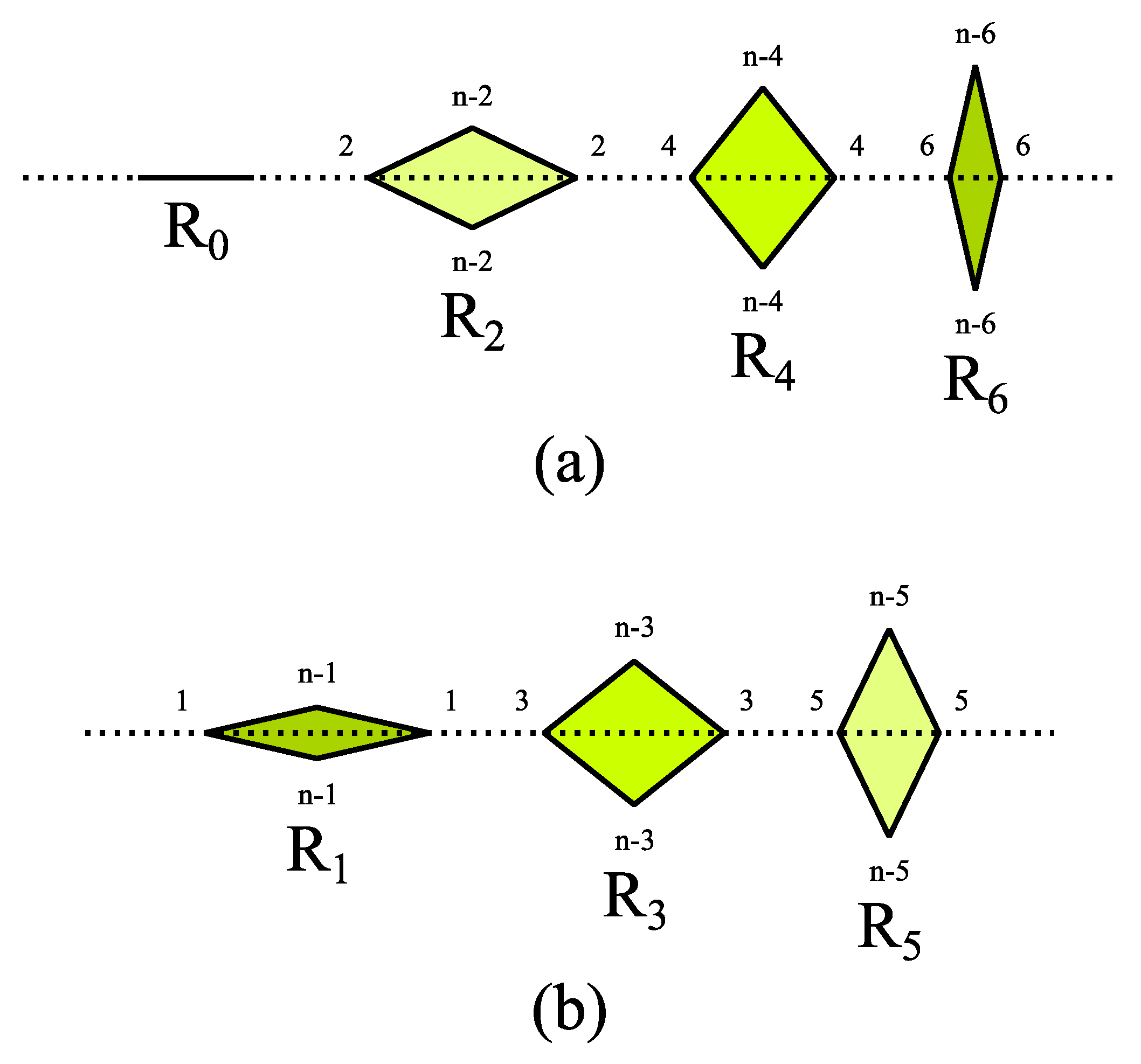
• There are two ways to place rhombs on the edge of substitution rules. We recall that the inner angles of the rhombs are integer multiples of $\frac{\pi }{n}$. We can place all rhombs on the edge so that the inner angles either with even or odd multiples of $\frac{\pi }{n}$ are bisected by the boundary of the supertile. We will call these two cases “even” and “odd edge configuration”, for details see Figure 7. A “mixed” configuration is not allowed, because it would force the existence of rhombs with inner angle equal to $\left(k+\frac{1}{2}\right)\frac{\pi }{n}$.
• We can choose the symmetry of the substitution rules and their edges. Possible choices are dihedral symmetry $D_1$ and $D_2$. Edges with dihedral symmetry $D_1$ can have the boundary of the supertile or its perpendicular bisector as line of symmetry. The smallest nontrivial solution for the latter case is the generalized Goodman-Strauss tiling [39]. Since this example does not provide individual dihedral symmetry $D_n$ or $D_{2n}$ in general, we will focus on the other case.
  Substitution rules of rhombs which appear on the edge of a substitution rule are forced to have the appropriate dihedral symmetry $D_1$ as well. This is also true for substitution rules of prototiles which lie on the diagonal, i.e., a line of symmetry of a substitution rule. The orientations of the edges have to be considered as well. These three conditions may force the introduction of additional rhomb prototiles and substitution rules. Additionally, the existence of edges with orientations may require additional preconditions.
  To avoid this problem, a general dihedral symmetry $D_2$ can be chosen for the substitution rules and their edges.
• Parity of the chosen n may require different approaches in some cases, similar to the example of the generalized Lançon-Billard tiling in Section 3.2 and Figure 4.

The options above can be combined without restrictions, so in total we have eight cases as shown in

Table 3. Definition of cases of rhombic CASTs.

	Substitution Rules and Their Edges Have at Least Dihedral Symmetry D1	Substitution Rules and Their Edges Have Dihedral Symmetry D2
Even edge configuration	Case 1a $(evenn)$ Case 1b $(oddn)$	Case 3a $(evenn)$ Case 3b $(oddn)$
Odd edge configuration	Case 2a $(evenn)$ Case 2b $(oddn)$	Case 4a $(evenn)$ Case 4b $(oddn)$

.

Within this section, we will denote a rhomb with side length $d_0\equiv 1$ and an inner angle $\frac{k\pi }{n}$, $n>k>0$ which is bisected by the boundary of a supertile as $R_k$ and its diagonal which lies on the boundary of a supertile as $d_k$. The line segments which appear on the edges of substitution rules in the cases with even edge configuration are denoted by $R_0$ and their length by $d_0$. Under those conditions, we can write the inflation multiplier η as sum of the $d_k$:

$$\eta ={\displaystyle \sum _{i=0}^{⌊(n-1)/2⌋}}{\alpha }_{2i}{d}_{2i}({\alpha }_k\in {\mathbb{N}}_0,cases1and3)$$

(81)

$$\eta ={\displaystyle \sum _{i=0}^{⌊n/2-1⌋}}{\alpha }_{2i+1}{d}_{2i+1}({\alpha }_k\in {\mathbb{N}}_0,cases2and4)$$

(82)

The inflation multiplier η can also be written as a sum of $2n$-th roots of unity, where the roots occur in pairs ${\zeta }_{2n}^i+\overline{{\zeta }_{2n}^i}$ so that $\eta \in \mathbb{R}$:

$$\eta ={\alpha }_0+{\displaystyle \sum _{i=0}^{⌊(n-1)/2⌋}}{\alpha }_{2i}\left({\zeta }_{2n}^i+\overline{{\zeta }_{2n}^i}\right)({\alpha }_k\in {\mathbb{N}}_0,\eta \in \mathbb{R},cases1and3)$$

(83)

$$\eta =\sqrt{2+{\zeta }_{2n}^1+\overline{{\zeta }_{2n}^1}}\left({\alpha }_1+{\displaystyle \sum _{i=0}^{⌊n/2-1⌋}}{\alpha }_{2i+1}\left({\zeta }_{2n}^i+\overline{{\zeta }_{2n}^i}\right)\right)({\alpha }_k\in {\mathbb{N}}_0,\eta \in \mathbb{R},cases2and4)$$

(84)

We borrow a remark regarding worms from [44]: “By definition, a parallelogram has two pairs of parallel edges. In a parallelogram tiling therefore there are natural lines of tiles linked each sharing a parallel edge with the next. These lines are called worms and were used by Conway in studying the Penrose tilings [2]. We will follow Conway to call these lines worms.”

Every rhomb $R_k$ with an inner angle $\frac{k\pi }{n}$, $n>k>0$ which is bisected by the boundary of a supertile work as entry-exit-node of two worms. We also can say that such a rhomb on the edge “reflects” a worm back into the substitution rule. The line segments $R_0$ work as entry-exit-node of one worm only.

The Kannan-Soroker-Kenyon (KSK) criterion as defined in [45,46] decides whether a polygon can be tiled by parallelograms. We use a simplified phrasing for the criterion: All line segments $R_0$ and all inner line segments of rhombs $R_k$, $n>k>0$ on the edge of the substitution rule serve as nodes. All corresponding nodes of the substitution rules are connected by lines. The KSK criterion is fulfilled if for every intersection of lines the inner angles between the corresponding nodes are larger than 0 and smaller than π.

We start with observations of the substitution rule for rhomb prototile $R_1$ or $R_{n-1}$. In detail we will focus on those both edges which enclose the inner angle equal $\frac{\pi }{n}$ and which we will denote as “corresponding edges”. We will denote the area where the both edges meet as the “tip” of the substitution rule.

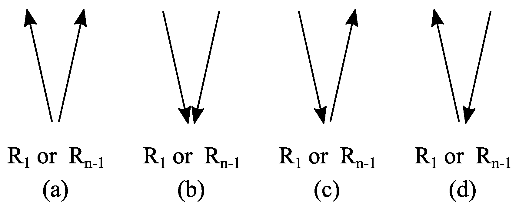
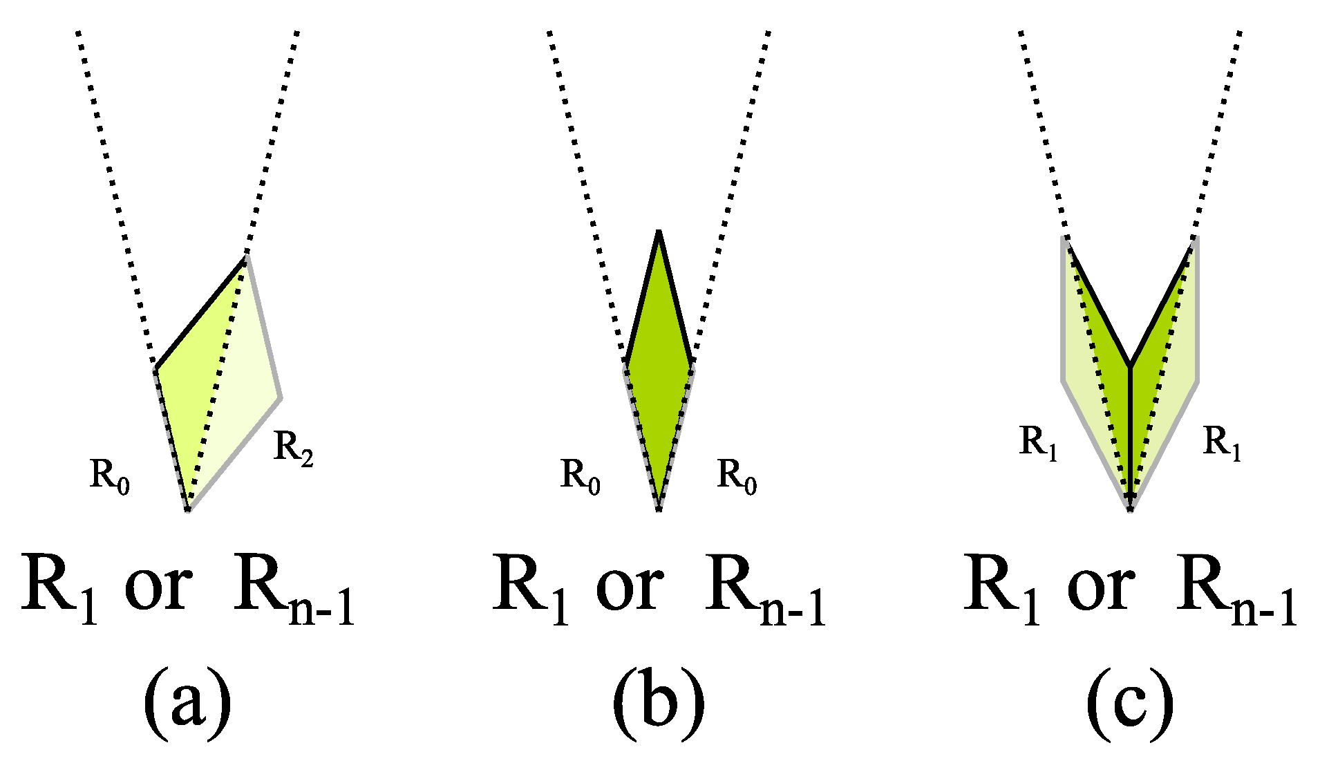
• The rhombs on the edges must not overlap. For this reason, for the tip of the substitution rule, only three configurations are possible as shown in Figure 8. Obviously, a tip as shown in Figure 8c is compliant to the cases 2 and 4 with odd edge configuration and Figure 8b to cases 1 and 3 with even edge configuration. Figure 8a requires the even edge configuration as well. Since all edges are congruent, it must be the start and the end of the same edge, which meet on that vertex. Since start and end of the edge are different, it can not have dihedral symmetry $D_2$. For this reason, the tip in Figure 8a is not compliant to case 3.
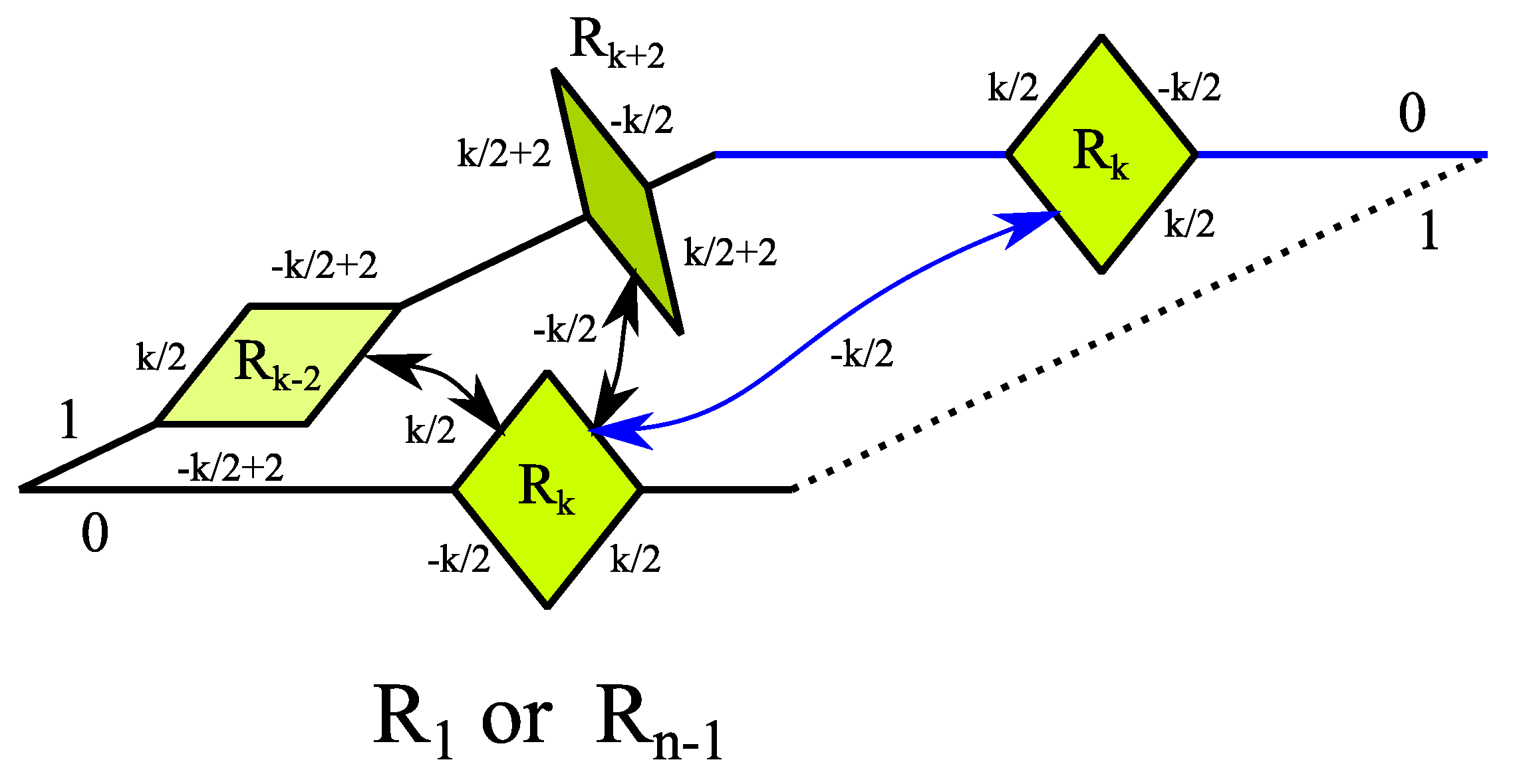
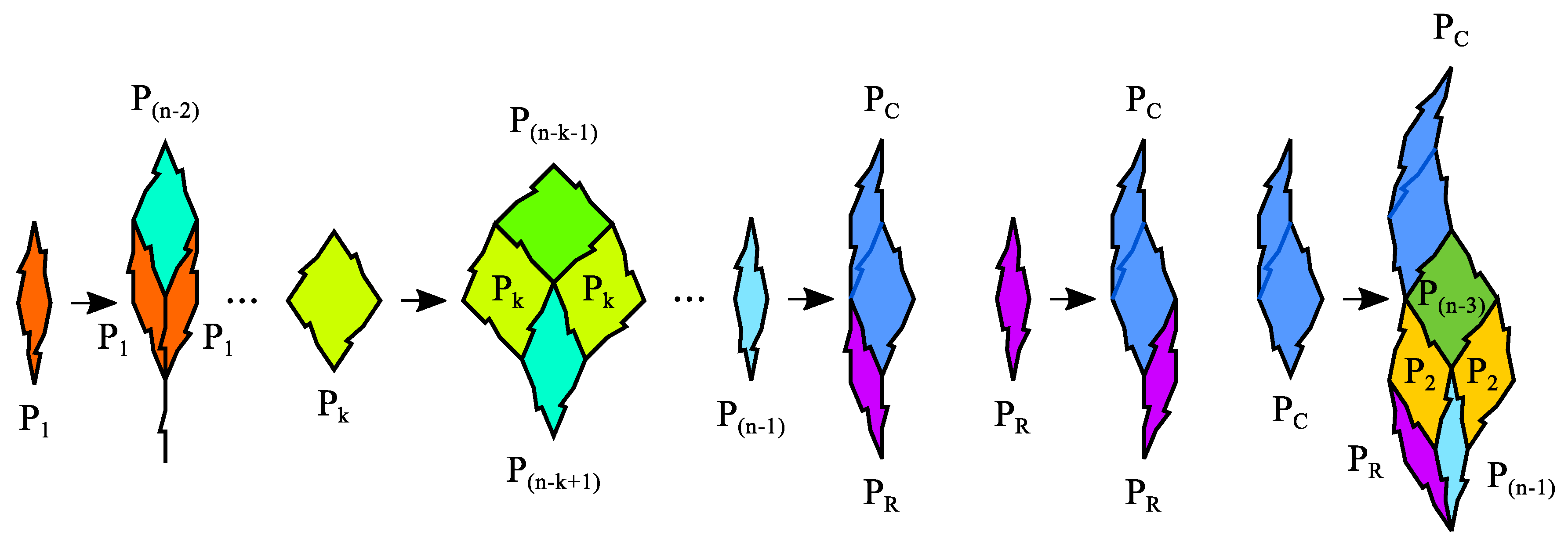
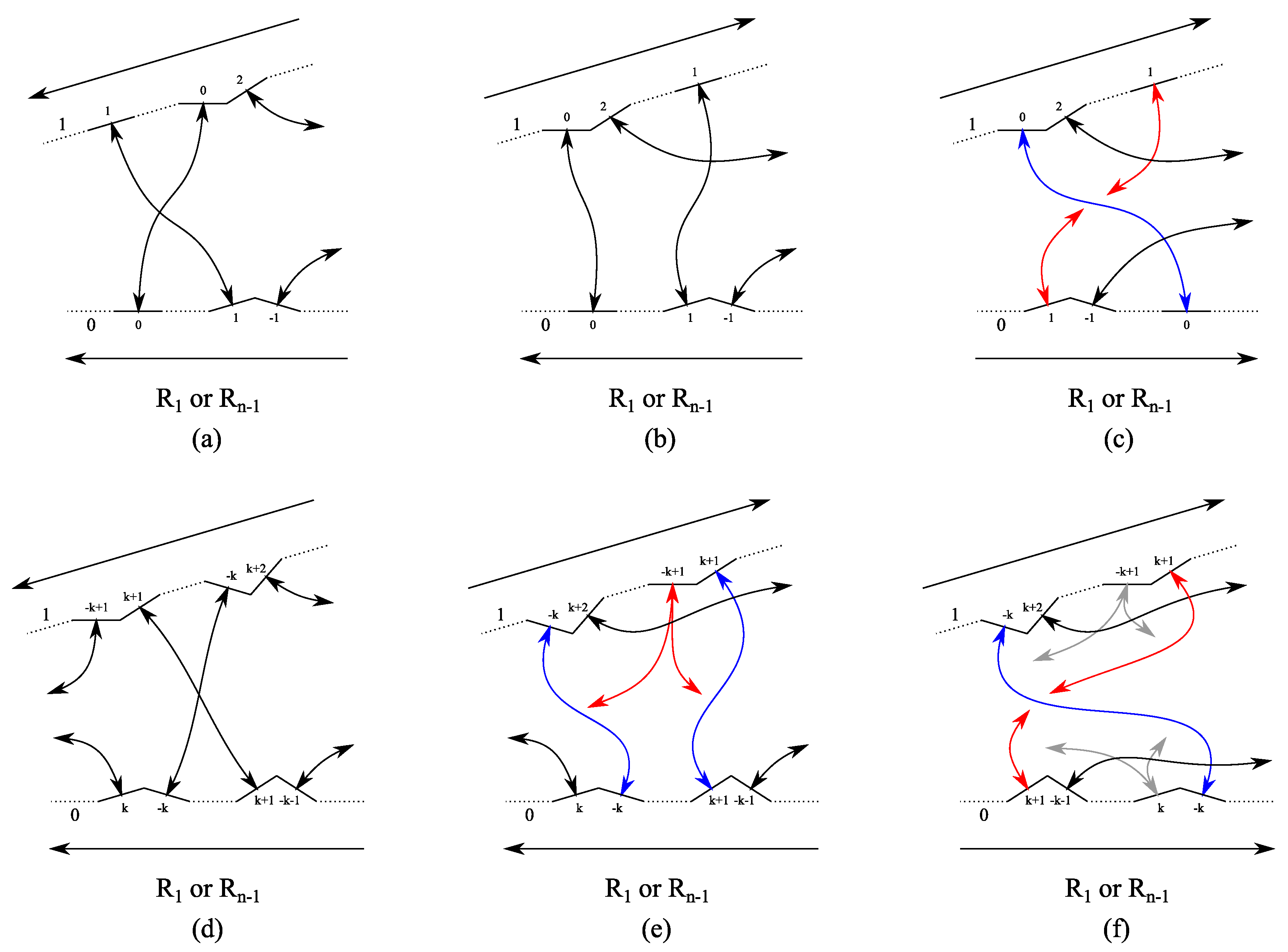
• Any rhomb $R_k$ with $n-3\ge k\ge 3$ on one edge implies the existence of a rhomb $R_{k-2}$ on the corresponding edge. In turn, rhomb $R_k$ on one edge is implied by a rhomb $R_{k+2}$ on the corresponding edge or a rhomb $R_k$ on the opposite edge. An example is shown in Figure 9.
• Any rhomb $R_2$ on one edge implies the existence of a line segment $R_0$ on the corresponding edge. In turn, rhomb $R_2$ on one edge is implied by a rhomb $R_4$ on the corresponding edge or a rhomb $R_2$ on the opposite edge.
• Any rhomb $R_1$ on one edge implies the existence of a rhomb $R_1$ on the corresponding edge. In turn, rhomb $R_1$ on one edge is implied by a rhomb $R_3$ on the corresponding edge or a rhomb $R_1$ on the opposite edge.
• Any line segment $R_0$ on one edge is implied by a rhomb $R_2$ on the corresponding edge or a line segment $R_0$ on the opposite edge.
• Any rhomb $R_{n-2}$ on one edge implies the existence of a rhomb $R_{n-4}$ on the corresponding edge. In turn, rhomb $R_{n-2}$ on one edge is implied by a rhomb $R_{n-2}$ on the opposite edge. (Rhomb $R_n$ does not exist, because the inner angle would be zero.)
• Any rhomb $R_{n-1}$ on one edge implies the existence of a rhomb $R_{n-3}$ on the corresponding edge. In turn, rhomb $R_{n-1}$ on one edge is implied by a rhomb $R_{n-1}$ on the opposite edge. (Rhomb $R_{n+1}$ does not exist, it would have an inner angle greater than π or smaller the 0.)
• If for a rhomb $R_k,n>k>0$ on one edge two related elements (rhomb or line segment) $R_{|k-2|}$ and $R_{k+2}$ exist on the corresponding edge, $R_{|k-2|}$ is closer to the tip than $R_{k+2}$.

Since all edges are congruent we can derive the following inequalities for ${\alpha }_k$:

$${\alpha }_0\ge {\alpha }_2\ge {\alpha }_4\ge \dots {\alpha }_{2⌊(n-1)/2⌋}\ge 0({\alpha }_k\in {\mathbb{N}}_0,cases1and3)$$

(85)

$${\alpha }_1\ge {\alpha }_3\ge {\alpha }_5\ge \dots {\alpha }_{2⌊n/2⌋-1}\ge 0({\alpha }_k\in {\mathbb{N}}_0,cases2and4)$$

(86)

Because of Equations (8) and (9), the inflation multiplier can also be written as a sum of diagonals ${\mu }_{n,k}$:

$$\eta ={\displaystyle \sum _{k=1}^{⌊n/2⌋}}{\beta }_k{\mu }_{n,k}({\beta }_k\in {\mathbb{N}}_0,cases1and3)$$

(87)

$$\eta =\sqrt{{\mu }_{n,2}+2}{\displaystyle \sum _{k=1}^{⌊n/2⌋}}{\beta }_k{\mu }_{n,k}({\beta }_k\in {\mathbb{N}}_0,cases2and4)$$

(88)

Equations (81)–(84) give no hint on which ${\alpha }_k=0$, so that a rhombic CAST still can exist. For this reason, we have to extend our observations to the substitution rules of rhomb $R_{⌊n/2⌋}$.

For case 1b and 3b:

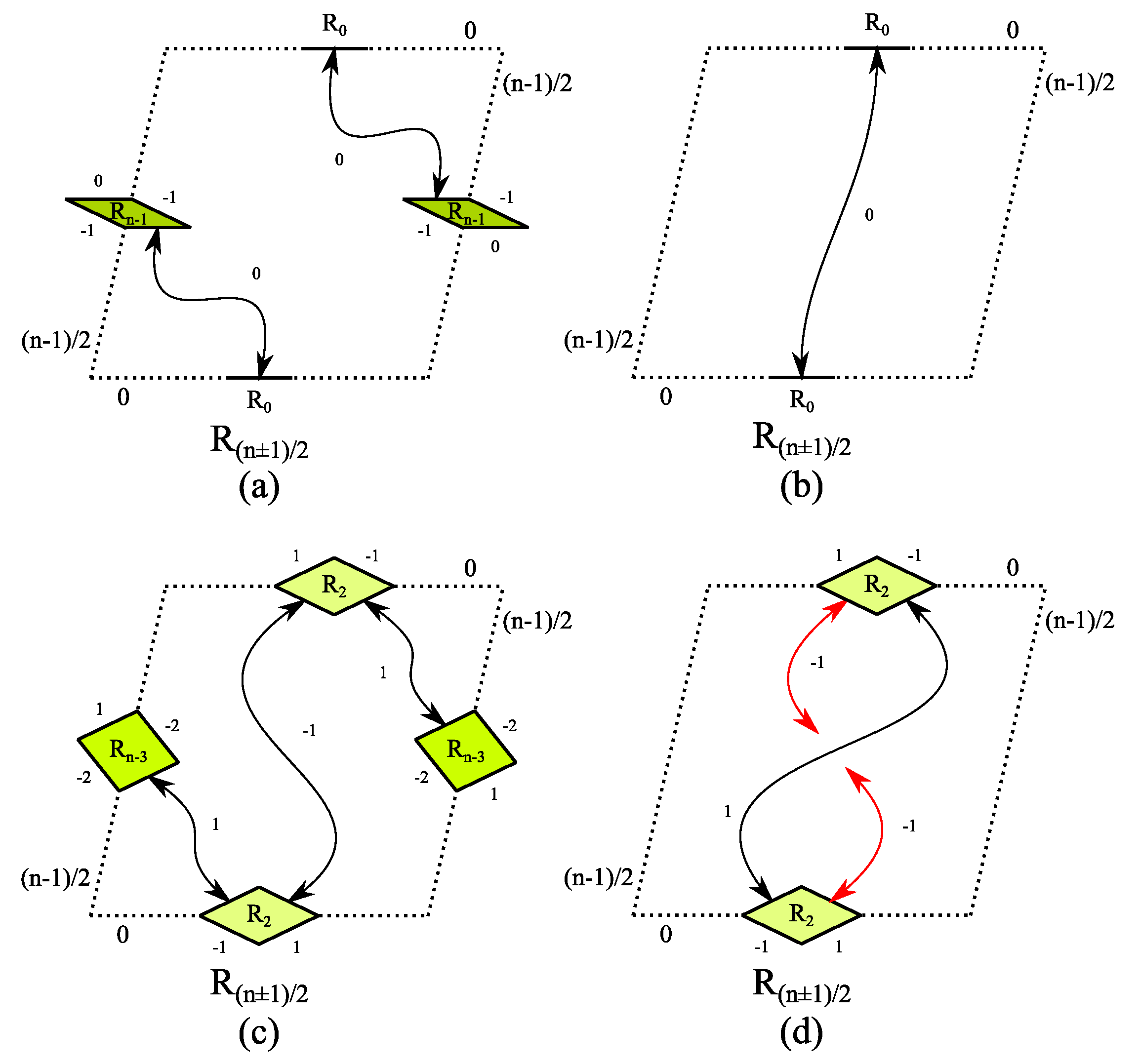
• Any line segment $R_0$ on the edge implies the existence of a rhomb $R_{n-1}$ on the correspondent edge or a line segment $R_0$ on the opposite edge. As shown in Figure 10a,b, the existence of rhomb $R_{n-1}$ on the edge is not required to meet the KSK criterion.
• Any rhomb $R_2$ on the edge implies the existence of a rhomb $R_{n-3}$ on the correspondent edge or a rhomb $R_2$ on the opposite edge. As shown in Figure 10c,d, the KSK criterion is only met if at least one $R_{n-3}$ exists on the edge.

  $${\alpha }_{n-3}>{\alpha }_{n-1}\ge 0(cases1band3b)$$

  (89)

For case 1a and 3a:

• The line segment $R_0$ on the edge implies the existence of a line segment $R_0$ on the opposite edge only (rhomb $R_n$ does not exist).
• Any rhomb $R_2$ on the edge implies the existence of a rhomb $R_{n-2}$ on the correspondent edge or a rhomb $R_2$ on the opposite edge. So the KSK criterion is only met if at least one $R_{n-2}$ exists on the edge.

  $${\alpha }_{n-2}\ge 1(cases1aand3a)$$

  (90)

For case 2b and 4b:

• Any rhomb $R_1$ on the edge implies the existence of a rhomb $R_{n-2}$ on the correspondent edge or a rhomb $R_1$ on the opposite edge. So the KSK criterion is only met if at least one $R_{n-2}$ exists on the edge.

  $${\alpha }_{n-2}\ge 1(cases2band4b)$$

  (91)

For case 2a and 4a:

• Any rhomb $R_1$ on the edge implies the existence of a rhomb $R_{n-1}$ on the correspondent edge or a rhomb $R_1$ on the opposite edge. So the KSK criterion is only met if at least one $R_{n-1}$ exists on the edge.

  $${\alpha }_{n-1}\ge 1(cases2aand4a)$$

  (92)

In the next part we will determine the minimal inflation multiplier ${\eta }_{min}$ of a rhombic CAST. We will discuss only case 1 in detail to show the general concept.

We continue our observations of the substitution rule $R_1$ or $R_{n-1}$. There are four possible combinations of the corresponding edge orientations as shown in Figure 11.

We recall Equations (85) and (89). To get a small inflation multiplier, the ${\alpha }_k$ with $evenk$ have to be chosen as small as possible. We use the KSK criterion to check whether substitution rules can exist for different orientations of the corresponding edges and equal amounts of rhombs $R_k$ and $R_{k+2}$ so that ${\alpha }_k={\alpha }_{k+2}$. The checks are illustrated in Figure 12. Actually, the figure just shows the case ${\alpha }_k={\alpha }_{k+2}=1$, while the result is true for ${\alpha }_k={\alpha }_{k+2}>1$ as well.

The results for ${\alpha }_0={\alpha }_2$ in Figure 12a–c show that the KSK criterion is fulfilled for more than one combination.

The results for ${\alpha }_k={\alpha }_{k+2};k>0$ in Figure 12d–f show that the KSK criterion is fulfilled for one orientation only.

At this point we have to introduce an additional condition. For cases 1 and 2, we consider only rhombic CASTs whose prototiles $R_1$ or $R_{n-1}$ yield at least two different orientations of the corresponding edges.

Remark 12.

The author is only aware of one example of a rhombic CAST whose prototiles $R_1$ or $R_{n-1}$ show only one orientation of the corresponding edges, namely the Ammann-Beenker tiling with $n=4$. For $n>4$, the existence of such rhombic CASTs seem to be unlikely. However, a proof to rule out this possibility is not available yet.

With the results and conditions above we can conclude:

$${\alpha }_0\ge {\alpha }_2(case1)$$

(93)

$${\alpha }_{2k}>{\alpha }_{2k+2};k>0(case1)$$

(94)

With Equations (9), (83), (85) and (87), we can describe the minimal inflation multiplier:

$${\eta }_{min}={\displaystyle \sum _{i=1}^{⌊n/2-1⌋}}\left({\mu }_{n,i}+{\mu }_{n,i+1}\right)(case1)$$

(95)

For case 1b with $oddn$, we can use the same concept of orientations as shown in [33] (Figure 2) which leads to rhombs with orientations as shown in Figure 13. As a result, the orientations of the edges are globally defined. In detail, the edges which enclose an inner angle $\frac{\pi }{n}$ have orientations as shown in Figure 11c,d and a tip as shown in Figure 8a.

For case 1a with $evenn$ this simplification can not be used. The edges which enclose an inner angle $\frac{\pi }{n}$ have not only orientations as shown in Figure 11c,d. Depending on how exactly the orientations are defined one of the orientations in Figure 11a or Figure 11b may appear.

Similar approaches are possible for cases 2, 3 and 4. For cases 3 and 4 the symmetry conditions of the substitution rules and its edges enforce ${\alpha }_{k}even,k>1$, just ${\alpha }_0$ is not required to be even.

With the minimal inflation multiplier ${\eta }_{min}$ as shown in

Table 4. Rhombic CAST substitution rule edge configuration for case 1.

n	Minimal Rhomb Edge Sequence	Minimal Inflation Multiplier ηmin
$4,5$	$\overline{0-2}$	${\mu }_{n,2}+1$
$6,7$	$\overline{0-2}-4-\overline{0-2}$	${\mu }_{n,3}+2{\mu }_{n,2}+1$
$8,9$	$\overline{0-2}-4-\overline{0-2}-6-4-\overline{0-2}$	${\mu }_{n,4}+2{\mu }_{n,3}+2{\mu }_{n,2}+1$
$10,11$	$\overline{0-2}-4-6-8-\overline{0-2}-4-\overline{0-2}-6-4-\overline{0-2}$	${\mu }_{n,5}+2{\mu }_{n,4}+2{\mu }_{n,3}+2{\mu }_{n,2}+1$
…	…	…

,

Table 5. Rhombic CAST substitution rule edge configuration for case 2.

n	Minimal Rhomb Edge Sequence	Minimal Inflation Multiplier ηmin
$4,5$	$1-3-1$	$\sqrt{{\mu }_{n,2}+2}\left({\mu }_{n,2}+2\right)$
$6,7$	$1-3-1-5-3-1$	$\sqrt{{\mu }_{n,2}+2}\left({\mu }_{n,3}+2{\mu }_{n,2}+2\right)$
$8,9$	$1-3-5-1-3-7-1-5-3-1$	$\sqrt{{\mu }_{n,2}+2}\left({\mu }_{n,4}+2{\mu }_{n,3}+2{\mu }_{n,2}+2\right)$
$10,11$	$1-3-5-7-1-3-1-5-9-3-1-7-5-3-1$	$\sqrt{{\mu }_{n,2}+2}\left({\mu }_{n,5}+2{\mu }_{n,4}+2{\mu }_{n,3}+2{\mu }_{n,2}+2\right)$
…	…	…

,

Table 6. Rhombic CAST substitution rule edge configuration for case 3.

n	Minimal Rhomb Edge Sequence	Minimal Inflation Multiplier ηmin
$4,5$	$0-2-0-2-0$	$2{\mu }_{n,2}+3$
$6,7$	$0-2-4-0-2-0-2-0-4-2-0$	$2{\mu }_{n,3}+4{\mu }_{n,2}+3$
$8,9$	$0-2-4-6-0-2-4-0-2-0-2-0-4-2-0-6-4-2-0$	$2{\mu }_{n,4}+4{\mu }_{n,3}+4{\mu }_{n,2}+3$
…	…	…

and

Table 7. Rhombic CAST substitution rule edge configuration for case 4.

n	Minimal Rhomb Edge Sequence	Minimal Inflation Multiplier ηmin
$4,5$	$1-3-1-1-3-1$	$\sqrt{{\mu }_{n,2}+2}\left(2{\mu }_{n,2}+4\right)$
$6,7$	$1-3-5-1-3-1-1-3-1-5-3-1$	$\sqrt{{\mu }_{n,2}+2}\left(2{\mu }_{n,3}+4{\mu }_{n,2}+4\right)$
$8,9$	$1-3-5-7-1-3-5-1-3-1-1-3-1-5-3-1-7-5-3-1$	$\sqrt{{\mu }_{n,2}+2}\left(2{\mu }_{n,4}+4{\mu }_{n,3}+4{\mu }_{n,2}+4\right)$
…	…	…

, we can start the search of rhombic CASTs by trial and error. The minimal rhomb edge sequences therein were also obtained in this way, so additional solutions with varied sequences obtained by permutation may exist. Examples for all eight cases are shown in Figure 14, Figure 15, Figure 16 and Figure 17:

Conjecture 4.

For all cases as listed in Table 3, there exist rhombic CASTs for any n with edge configuration and inflation multiplier ${\eta }_{min}$ as shown in Table 4, Table 5, Table 6 and Table 7 which yield individual dihedral symmetry $D_n$ or $D_{2n}$.

A general proof of Conjecture 4 is subject to further research. However, a proof for case 4b already exists. The results in [47] for $oddn$ match very well with our results in case 4b. The case $evenn$ in the same publication is almost identical to our case 3a, up to a difference of one line segment $R_0$ in the center of the edge of the substitution rules.

Remark 13.

Case 1a with $n=4$ is equivalent to the Ammann-Beenker tiling [10,32,48,49].

Remark 14.

Socolar’s 7-fold tiling [32] (credited to J. Socolar) can be derived from case 1b with $n=7$ with a modified minimal rhomb edge sequence.

Remark 15.

Two substitution steps of the Penrose rhomb tiling are equivalent to one substitution step in case 1b with $n=5$.

6. Gaps to Prototiles Algorithm

In this section, we sketch a “Gaps to Prototiles” algorithm to identify CASTs for a given n and a selected edge of a substitution rule (as in Definition 2).

Conditions:

• All prototiles have inner angles equal $\frac{k\pi }{n}$.
• All edges of all substitution rules are congruent and have dihedral symmetry $D_2$.
• As discussed in Section 5 the tiles on the edge have to be placed, so that the inner angles either with even or odd multiples of $\frac{\pi }{n}$ are bisected by the boundary of the supertile.
• The tiles on the edge are bisected by one or two lines of symmetry of the edge. This implies dihedral symmetry $D_1$ or $D_2$ of the corresponding substitution rules.
• The inflation multiplier η must fulfill the conditions in Theorem 1.
• The inflation multiplier η is defined by the sequence of tiles which are part of the edge.

Algorithm:

• We start with the prototiles which appear on the edge of the substitution rule.
• We start the construction of the substitution rules by placing the prototiles on the edge.
• If the edge prototiles overlap the algorithm has failed. In this case, we may adjust the sequence of rhombs or other equilateral polygons on the edge and start another attempt.
• We try to “fill up” the substitution rules with existing prototiles under consideration of the appropriate dihedral symmetry $D_1$ or $D_2$. If gaps remain, they are defined as new prototiles and we go back to step (2). Please note, if a gap lies on one or two lines of symmetry, the substitution rule of the new prototile must also have the appropriate dihedral symmetry $D_1$ or $D_2$.
• If no gaps remain the algorithm was successful.

In some cases the “Gaps to Prototiles” algorithm delivers results with preferable properties as shown in Figure 18, Figure 19 and Figure 20 and inflation multipliers as shown in

Table 8. Inflation multipliers of CASTs identified by the “Gaps to Prototiles” algorithm.

n	Inflation Multiplier	Corresponding Figure
7	$2{\mu }_{7,3}+2{\mu }_{7,2}+1$	Figure 18
7	${\mu }_{7,2}+2$	Figure 19
4	$\sqrt{{\mu }_{4,2}+2}$	Figure 20

. However, some results contain a very large number of prototiles with different sizes and complex shapes as in Figure 19. It is not known yet whether the algorithm always delivers solutions with a finite number of prototiles.

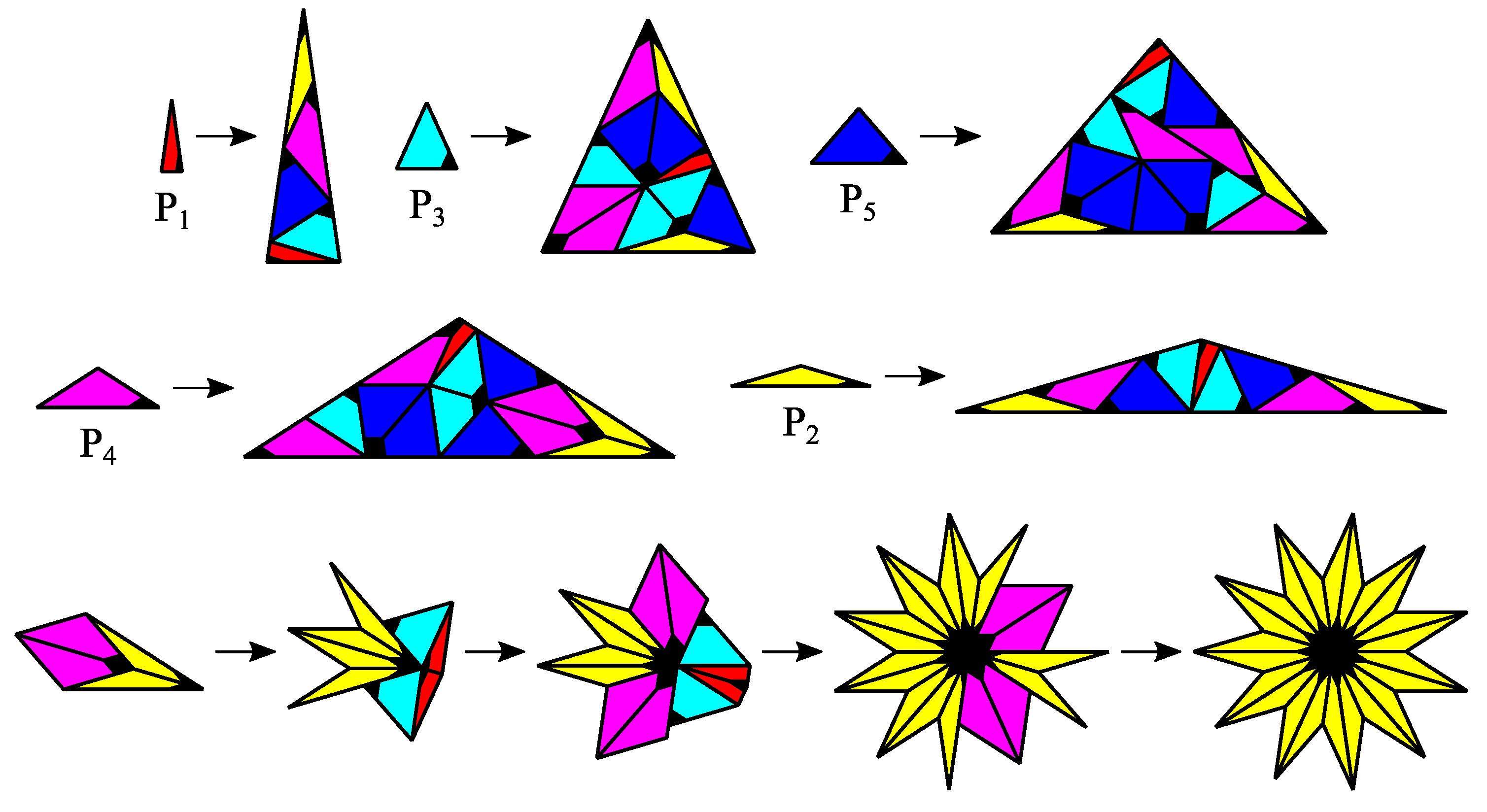
7. Extended Girih CASTs

“Girih” is the Persian word for “knot” and stands for complex interlaced strap works of lines, which are a typical feature of Islamic architecture and design. A common definition is given in [50]: “Geometric (often star-and-polygon) designs composed upon or generated from arrays of points from which construction lines radiate and at which they intersect.” The oldest known examples of star pattern date back to the 8th century AD [51]. Girih designs are known in many styles and symmetries, see [52] for examples. A variant of Girih design relies on Girih tiles and tilings as shown in the reproduction of the Topkapi Scroll in [53]. The decorations on the tiles consist of lines which run from tile to tile when they are joined together. So the borders between joined tiles seem to disappear.

According to [53] the shapes of all girih tiles are equilateral polygons with the same side length and inner angles $\frac{k\pi }{5}$, $k\in \{2,3,4,6\}$ including:

• Regular decagon with inner angles $\frac{4\pi }{5}$
• Regular pentagon with inner angles $\frac{3\pi }{5}$
• Rhomb with inner angles $\frac{2\pi }{5}$ and $\frac{3\pi }{5}$
• Convex hexagon with inner angles $\frac{2\pi }{5}$,$\frac{4\pi }{5}$,$\frac{4\pi }{5}$,$\frac{2\pi }{5}$,$\frac{4\pi }{5}$,$\frac{4\pi }{5}$
• Convex hexagon with inner angles $\frac{3\pi }{5}$,$\frac{3\pi }{5}$,$\frac{4\pi }{5}$,$\frac{3\pi }{5}$,$\frac{3\pi }{5}$,$\frac{4\pi }{5}$
• Nonconvex hexagon with inner angles $\frac{2\pi }{5}$, $\frac{2\pi }{5}$, $\frac{6\pi }{5}$, $\frac{2\pi }{5}$, $\frac{2\pi }{5}$, $\frac{6\pi }{5}$

Because of these properties, Girih tilings are cyclotomic tilings as well.

A Girih (cyclotomic) aperiodic substitution tiling was derived from a mosaic at the Darb-i Imam Shrine, Isfahan, Iran which dates back from 1453. It relies on the regular decagon and two hexagons and has individual dihedral symmetry $D_{10}$. It was published in [54]. However, the complete set of substitution rules can be found in [55,56]. Additional examples of Girih CASTs have been discovered and submitted to [32]. More examples have been published in [56,57,58].

That rises the question if Girih CASTs with other symmetries and relative small inflation multiplier exist. For this reasons we have to define the extended Girih CASTs. The following definition turned out to be useful for a given $n\ge 4$.

• All prototiles of an extended Girih CAST are equilateral polygons with the same side length.
• The inner angles of all prototiles are $\frac{k\pi }{n}$, $k\in \left\{2,3\dots \left(n-1\right),\left(n+1\right),\left(n+2\right)\dots \left(n-2\right)\right\}$.
• One of the prototiles may be a regular n-gon with inner angles $\frac{\left(n-2\right)\pi }{n}$.
• One of the prototiles may be a regular $2n$-gon with inner angles $\frac{\left(n-1\right)\pi }{n}$.

Please note that prototiles with inner angle $\frac{\pi }{n}$ are forbidden due to aesthetic reasons.

For the extended Girih CASTs in this section we choose the following properties:

• All edges of the substitution rules are congruent and have dihedral symmetry $D_2$.
• All substitution rules except those for regular n-gons with $oddn$ have dihedral symmetry $D_2$.
• The substitution rule of the regular n-gon with $oddn$ has dihedral symmetry $D_1$.
• The substitution rule of the regular $2n$-gon has dihedral symmetry $D_{2n}$ for $oddn$ and $D_n$ for $evenn$.

Examples for extended Girih CASTs in this section with $n\in \left\{4,5,7\right\}$ are shown in Figure 21, Figure 22, Figure 23 and Figure 24 and its corresponding eigenvalues are shown in

Table 9. Inflation multipliers of extended Girih CASTs.

n	Inflation Multiplier	Corresponding Figure
4	${\mu }_{4,2}+1$	Figure 21
5	$\sqrt{{\mu }_{5,2}+2}({\mu }_{5,2}+1)$	Figure 22
5	$2({\mu }_{5,2}+1)$	Figure 23
7	${\mu }_{7,2}+2{\mu }_{7,1}+2$	Figure 24

.

The Girih CASTs in Figure 21, Figure 22 and Figure 24 have been obtained by a trial and error method under the following conditions:

• In every corner of every substitution rule a regular $2n$-gon is placed.
• Edge and inflation multiplier have been derived from a periodic pattern of regular $2n$-gons and their inter space counterparts.

For $n\ge 8$ this approach might fail. As an alternative it is possible to reuse inflation multipliers from rhombic CASTs in Section 5, case 1 and 2. See Table 4 and Table 5 for details.

The Girih CAST in Figure 23 has been derived from [56] (Figures 14 and 15). In detail the nonconvex hexagons were replaced and the star shaped gap in the center of the substitution rule of the pentagon prototile [56] (Figure 15b) was eliminated. This was possible by changing the symmetry of the substitution rule from dihedral symmetry $D_5$ to $D_1$. The tilings in [56] (Figures 14 and 15) were derived by an analysis of patterns shown in the Topkapi Scroll, in detail [53] (Panels 28, 31, 32, 34).

Remark 16.

Please note that the case $evenn$ requires special care to make sure that the regular $2n$-gons with dihedral symmetry $D_n$ always match. It seems that the existence of a substitution rule of the regular $2n$-gons with dihedral symmetry $D_{2n}$ requires the existence of prototiles with inner angle $\frac{\pi }{n}$ which are forbidden due to our preconditions. As a result, additional substitution rules might be necessary for prototiles with the same shape but different orientations.

Remark 17.

The decorations at the prototiles are related but not necessarily equivalent to Ammann bars.

8. Summary and Outlook

Although the motivation behind this article was mainly aesthetic, some significant results have been achieved. Cyclotomic Aperiodic Substitution Tilings (CASTs) cover a large number of new and well known aperiodic substitution tilings as shown in

Table 10. Inflation multipliers and individual symmetry of some CASTs.

n	Name	Inflation Multiplier	Patches with Individual Symmetry	Reference
5	Penrose	${\mu }_{5,2}$	$D_5$	[27,28,29,32] [2] (Chapter 10.3) [3] (Chapter 6.2)
7	Danzer’s 7-fold variant	${\mu }_{7,2}$	$D_7$	[33] (Figure 1 and Section 3, 2nd matrix) Herein Figure 3
7	Danzer’s 7-fold variant (two variants)	${\mu }_{7,3}$	$D_1$	[32] (credited to L. Danzer)
			$D_7$	[33] (Figure 11)
7	Math Pages 7-fold	${\mu }_{7,3}$	-	[41]
9	Math Pages 9-fold	${\mu }_{9,4}$	$D_9$	[41]
5	Lançon-Billard / Binary	$\sqrt{{\mu }_{5,2}+2}$	-	[32,37,38] [3] (Chapter 6.5.1)
6	Shield	$\sqrt{{\mu }_{6,2}+2}$	-	[32,59,60] [3] (Chapter 6.3.2)
4	Ammann-Beenker	${\mu }_{4,2}+1$	$D_8$	[10,32,48,49] [2] (Chapter 10.4) [3] (Chapter 6.1)
5	Tie and Navette / Bowtie-Hexagon 1	${\mu }_{5,2}+1$	-	[57,58] [22] (Section 8.2, Figure 8.3) [32] [56] (Figure 25)
5	Bowtie-Hexagon-Decagon 1	${\mu }_{5,2}+1$	$C_5$	[32] (credited to L. Andritz)
7	Danzer’s 7-fold (two variants)	${\mu }_{7,2}+1$	$D_1$	[33] (Figure 12) [32] [3] (Chapter 6.5.2)
7	Franco-Ferreira-da-Silva 7-fold	${\mu }_{7,2}+1$	$D_7$	[61]
7	Maloney’s 7-fold	${\mu }_{7,2}+1$	$D_7$	[32] [62] (Figure 9)
7	Cyclotomic Trapezoids	${\mu }_{n,2}+1$	$D_1$	[32,63]
9
11
4	Watanabe-Ito-Soma 8-fold	${\mu }_{4,2}+2$	$D_8$	[32,64,65,66]
4	Generalized Goodman-Strauss rhomb	${\mu }_{n,2}+2$	$D_1$	[39] [32] (credited to C. Goodman-Strauss and E. O. Harris)
5			$C_5$,$D_1$
$\ge 6$			$D_1$
6	Watanabe-Soma-Ito 12-fold (variants)	${\mu }_{6,2}+2$	$D_{12}$	[32,66]
6	Socolar	${\mu }_{6,2}+2$	$D_2$	[10,32,67]
6	Stampfli-Gähler / Ship	${\mu }_{6,2}+2$	$D_{12}$	[59,68,69]
6	Square Triangle	${\mu }_{6,2}+2$	$D_6$	[70,71,72,73] [32] (credited to M. Schlottmann) [3] (Chapter 6.3.1)
5	Cromwell	${\mu }_{5,2}+3$	$D_{10}$	[56] (Figures 12 and 13)
5	Topkapi Scroll	$2{\mu }_{5,2}+2$	$D_{10}$	Herein Figure 23, derived from [56] (Figures 14 and 15) and patterns shown in the Topkapi Scroll, in detail [53] (Panels 28, 31, 32, 34)
5	Bowtie-Hexagon-Decagon 2	$2{\mu }_{5,2}+3$	$C_5$	[32] (credited to L. Andritz)
5	Bowtie-Hexagon-Decagon 3	$3{\mu }_{5,2}+2$	$C_5$	[32] (credited to L. Andritz)
5	Darb-i Imam Shrine	$4{\mu }_{5,2}+2$	$D_{10}$	[54,55] [56] (Figure 21)
7	Franco’s 7-fold	${\mu }_{7,3}+{\mu }_{7,2}+1$	$D_7$	[74]
7	Gähler-Kwan-Maloney 7-fold	${\mu }_{7,3}+{\mu }_{7,2}+1$	$D_7$	[62] (Figure 10)
7	Socolar’s 7-fold	${\mu }_{7,3}+2{\mu }_{7,2}+1$	$D_7$	[32] (credited to J. Socolar)
9	Franco-da-Silva-Inácio 9-fold	${\mu }_{9,4}+{\mu }_{9,3}+{\mu }_{9,2}+1$	$D_9$	[75]
11	Maloney’s 11-fold	$3{\mu }_{11,5}+2{\mu }_{11,4}+2{\mu }_{11,3}+2{\mu }_{11,2}+1$	$D_{11}$	[8]

. The properties of CASTs, in detail their substitution matrices and their minimal inflation multipliers, can be used as practical starting point to identify previously unknown solutions. For many cases, such solutions yield individual dihedral symmetry $D_n$ or $D_{2n}$.

The different approaches to identify CASTs have their individual advantages and disadvantages. The preferable properties as listed in the introduction section may be complemented by a high frequency of patches with dihedral symmetry. A promising approach we do not discuss in this article may be the choice of inflation multipliers which are PV numbers.

The results in this paper focus strictly on the Euclidean plane so that Equation (4) applies. However, the methods described herein might be adapted for other cases as well.

Finally, several conjectures have been made, which require further research.

References

- Shechtman, D.; Blech, I.; Gratias, D.; Cahn, J.W. Metallic Phase with Long-Range Orientational Order and No Translational Symmetry. Phys. Rev. Lett. 1984, 53, 1951–1953. [Google Scholar] [CrossRef]
- Grünbaum, B.; Shephard, G.C. Tilings and Patterns; W. H. Freeman & Co.: New York, NY, USA, 1987. [Google Scholar]
- Baake, M.; Grimm, U. Aperiodic Order. Vol 1. A Mathematical Invitation. In Encyclopedia of Mathematics and Its Applications; Cambridge University Press: Cambridge, UK, 2013; Volume 149. [Google Scholar]
- Escher, M.C.; Bool, F.; Locher, J.L. M. C. Escher, His Life and Complete Graphic Work: With a Fully Illustrated Catalogue; H. N. Abrams: New York, NY, USA, 1982. [Google Scholar]
- Voderberg, H. Zur Zerlegung der Umgebung eines ebenen Bereiches in kongruente. Jahresber. Deutsch. Math. Ver. 1936, 46, 229–231. [Google Scholar]
- Voderberg, H. Zur Zerlegung der Ebene in kongruente Bereiche in Form einer Spirale. Jahresber. Deutsch. Math. Ver. 1937, 47, 159–160. [Google Scholar]
- Lück, R. Dürer-Kepler-Penrose, the development of pentagon tilings. Mater. Sci. Eng. A 2000, 294–296, 263–267. [Google Scholar] [CrossRef]
- Maloney, G.R. On substitution tilings of the plane with n-fold rotational symmetry. Discret. Math. Theor. Comput. Sci. 2015, 17, 395–412. [Google Scholar]
- Berger, R. The undecidability of the domino problem. Mem. Am. Math. Soc. 1966, 66, 1–72. [Google Scholar] [CrossRef]
- Socolar, J.E.S. Simple octagonal and dodecagonal quasicrystals. Phys. Rev. B 1989, 39, 10519–10551. [Google Scholar] [CrossRef]
- Socolar, J.E.S. Weak matching rules for quasicrystals. Commun. Math. Phys. 1990, 129, 599–619. [Google Scholar] [CrossRef]
- Gähler, F. Matching rules for quasicrystals: The composition-decomposition method. J. Non-Cryst. Solids 1993, 153, 160–164. [Google Scholar] [CrossRef]
- De Bruijn, N.G. Algebraic theory of Penrose’s non-periodic tilings of the plane I and II. Indag. Math. New Ser. 1981, 84, 39–66. [Google Scholar] [CrossRef]
- Lagarias, J.C. Meyer’s concept of quasicrystal and quasiregular sets. Commun. Math. Phys. 1996, 179, 365–376. [Google Scholar] [CrossRef]
- Moody, R.V. The Mathematics of Long-Range Aperiodic Order; Springer: Heidelberg, Germany, 1997. [Google Scholar]
- Meyer, Y. Algebraic Numbers and Harmonic Analysis; Elsevier: Amsterdam, The Netherlands, 1972. [Google Scholar]
- De Bruijn, N.G. Dualization of multigrids. J. Phys. Colloq. 1986, 47 (C3), 9–18. [Google Scholar] [CrossRef]
- Gähler, F.; Rhyner, J. Equivalence of the generalised grid and projection methods for the construction of quasiperiodic tilings. J. Phys. A Math. Gen. 1986, 19, 267. [Google Scholar] [CrossRef]
- Ingalls, R. Decagonal quasicrystal tilings. Acta Crystallogr. Sect. A 1992, 48, 533–541. [Google Scholar] [CrossRef]
- Ingalls, R. Octagonal quasicrystal tilings. J. Non-Cryst. Solids 1993, 153–154, 177–180. [Google Scholar] [CrossRef]
- Lück, R. Basic ideas of ammann bar grids. Int. J. Mod. Phys. B 1993, 7, 1437–1453. [Google Scholar] [CrossRef]
- Scheffer, M. Festkörperreaktionen in Quasikristallinen Legierungen. Ph.D. Thesis, Universität Stuttgart and Max-Planck-Institut für Metallforschung, Stuttgart, Germany, 1998. [Google Scholar]
- Von Koch, H. Sur une courbe continue sans tangente, obtenue par une construction géométrique élémentaire. Ark. Mat. 1904, 1, 681–702. [Google Scholar]
- Von Koch, H. Une méthode géométrique élémentaire pour l’étude de certaines questions de la théorie des courbes planes. Acta Math. 1906, 30, 145–174. [Google Scholar] [CrossRef]
- Mandelbrot, B.B. The Fractal Geometry of Nature; W. H. Freeman and Co.: San Francisco, CA, USA, 1977. [Google Scholar]
- Gardner, M. On ‘Rep-tiles’, Polygons that can make larger and smaller copies of themselves. Sci. Am. 1963, 208, 154–164. [Google Scholar] [CrossRef]
- Penrose, R. The role of aesthetics in pure and applied mathematical research. Bull. Inst. Math. Appl. 1974, 10, 266ff. [Google Scholar]
- Gardner, M. Extraordinary nonperiodic tiling that enriches the theory of tiles. Sci. Am. 1977, 236, 110–119. [Google Scholar] [CrossRef]
- Penrose, R. Pentaplexity A Class of Non-Periodic Tilings of the Plane. Math. Intell. 1979, 2, 32–37. [Google Scholar] [CrossRef]
- Goodman-Strauss, C. Matching Rules and Substitution Tilings. Ann. Math. 1998, 157, 181–223. [Google Scholar] [CrossRef]
- Goodman-Strauss, C. Matching Rules for the Sphinx Substitution Tiling. Unpublished Notes. Available online: http://comp.uark.edu/~strauss/ (accessed on 22 June 2016).
- Frettlöh, D.; Gähler, F.; Harris, E.O. Tilings Encyclopedia. Available online: http://tilings.math.uni-bielefeld.de/ (accessed on 22 June 2016).
- Nischke, K.P.; Danzer, L. A construction of inflation rules based on n-fold symmetry. Discret. Comput. Geom. 1996, 15, 221–236. [Google Scholar] [CrossRef]
- Steinbach, P. Golden fields: A case for the heptagon. Math. Mag. 1997, 70, 22–31. [Google Scholar] [CrossRef]
- Frettlöh, D. About substitution tilings with statistical circular symmetry. Philos. Mag. 2008, 88, 2033–2039. [Google Scholar] [CrossRef]
- Frettlöh, D.; Say-Awen, A.L.D.; de las Peñas, M.L.A.N. Substitution tilings with dense tile orientations and n-fold rotational symmetry. Indag. Math. 2016, in press. [Google Scholar]
- Lançon, F.; Billard, L. Two-dimensional system with a quasi-crystalline ground state. J. Phys. 1988, 49, 249–256. [Google Scholar] [CrossRef]
- Godrèche, C.; Lançon, F. A simple example of a non-Pisot tiling with five-fold symmetry. J. Phys. I 1992, 2, 207–220. [Google Scholar] [CrossRef]
- Harriss, E.O. Non-Periodic Rhomb Substitution Tilings that Admit Order n Rotational Symmetry. Discret. Comput. Geom. 2005, 34, 523–536. [Google Scholar] [CrossRef]
- Hibma, T. Generalization of Non-periodic Rhomb Substitution Tilings. arXiv, 2015; arXiv:1509.02053. [Google Scholar]
- Math Pages. Non-Periodic Tilings with n-fold Symmetry. Available online: http://mathpages.com/home/kmath539/kmath539.htm (accessed on 22 June 2016).
- Hibma, T. Aperiodic Rhomb Tiling. Available online: http://www.hibma.org/wpaperiodictiling/ (accessed on 22 June 2016).
- Warrington, D.H. Two Dimensional Inflation Patterns and Corresponding Diffraction Patterns. In Quasicrystalline Materials: Proceedings of the I.L.L./CODEST Workshop; Janot, C., Dubois, J., Eds.; World Scientific: Singapore, 1988; pp. 243–254. [Google Scholar]
- Frettlöh, D.; Harriss, E.O. Parallelogram Tilings, Worms, and Finite Orientations. Discret. Comput. Geom. 2013, 49, 531–539. [Google Scholar] [CrossRef]
- Kannan, S.; Soroker, D. Tiling Polygons with Parallelograms. Discret. Comput. Geom. 1992, 7, 175–188. [Google Scholar] [CrossRef]
- Kenyon, R. Tiling a Polygon with Parallelograms. Algorithmica 1993, 9, 382–397. [Google Scholar] [CrossRef]
- Kari, J.; Rissanen, M. Sub Rosa, A System of Quasiperiodic Rhombic Substitution Tilings with n-Fold Rotational Symmetry. Discret. Comput. Geom. 2016, 55, 972–996. [Google Scholar] [CrossRef]
- Beenker, F.P.M. Algebraic Theory of Non-Periodic Tilings of the Plane by Two Simple Building Blocks: A Square and a Rhombus; Technical Report 82-WSK04; Eindhoven University of Technology: Eindhoven, The Netherlands, 1982. [Google Scholar]
- Ammann, R.; Grünbaum, B.; Shephard, G.C. Aperiodic Tiles. Discret. Comput. Geom. 1992, 8, 1–25. [Google Scholar] [CrossRef]
- Allen, T. Islamic Art and the Argument from Academic Geometry; Solipsist Press: Occidental, CA, USA, 2004. [Google Scholar]
- Lee, A.J. Islamic Star Patterns. Muqarnas 1987, 4, 182–197. [Google Scholar] [CrossRef]
- Bourgoin, J. Arabic Geometrical Pattern and Design; Dover Pictorial Archive Series; Dover Publications: New York, NY, USA, 1973. [Google Scholar]
- Necipoğlu, G.; Al-Asad, M. The Topkapı Scroll: Geometry and Ornament in Islamic Architecture: Topkapı Palace Museum Library MS; Number Bd. 1956 in Sketchbooks & Albums; Getty Center for the History of Art and the Humanities: Santa Monica, CA, USA, 1995. [Google Scholar]
- Lu, P.J.; Steinhardt, P.J. Decagonal and Quasi-Crystalline Tilings in Medieval Islamic Architecture. Science 2007, 315, 1106–1110. [Google Scholar] [CrossRef] [PubMed]
- Tennant, R. Medieval Islamic Architecture, Quasicrystals, and Penrose and Girih Tiles: Questions from the Classroom. In Bridges Leeuwarden: Mathematics, Music, Art, Architecture, Culture; Sarhangi, R., Séquin, C.H., Eds.; Tarquin Publications: London, UK, 2008; pp. 297–304. Available online: http://archive.bridgesmathart.org/2008/bridges2008-297.html (accessed on 22 June 2016).
- Cromwell, P.R. The Search for Quasi-Periodicity in Islamic 5-fold Ornament. Math. Intell. 2008, 31, 36–56. [Google Scholar] [CrossRef]
- Lück, R. Penrose sublattices. J. Non-Cryst. Solids 1990, 117, 832–835. [Google Scholar] [CrossRef]
- Lück, R.; Lu, K. Non-locally derivable sublattices in quasi-lattices. J. Alloys Comp. 1994, 209, 139–143. [Google Scholar] [CrossRef]
- Gähler, F. Crystallography of Dodecagonal Quasicrystals. In Quasicrystalline Materials: Proceedings of the I.L.L./CODEST Workshop; Janot, C., Dubois, J., Eds.; World Scientific: Singapore, 1988; pp. 272–284. [Google Scholar]
- Niizeki, N.; Mitani, H. Two-dimensional dodecagonal quasilattices. J. Phys. A Math. Gen. 1987, 20, L405. [Google Scholar] [CrossRef]
- Franco, B.J.O.; Ferreira, J.R.F.; da Silva, F.W.O. A Third-Order Fibonacci Sequence Associated to a Heptagonal Quasiperiodic Tiling of the Plane. Phys. Status Solidi 1994, 182, K57–K62. [Google Scholar] [CrossRef]
- Gähler, F.; Kwan, E.E.; Maloney, G.R. A computer search for planar substitution tilings with n-fold rotational symmetry. Discret. Comput. Geom. 2015, 53, 445–465. [Google Scholar] [CrossRef]
- Frettlöh, D. Inflationäre Pflasterungen der Ebene Mit D2m+1-Symmetrie und Minimaler Musterfamilie, Betreuer Ludwig Danzer. Diploma Thesis, Universität Dortmund, Dortmund, Germany, 1998. [Google Scholar]
- Watanabe, Y.; Ito, M.; Soma, T.; Betsumiya, T. Nonperiodic Tesselation with Eight-Fold Rotational Symmetry. In Science on Form: Proceedings of the First International Symposium for Science on Form; Ishizaka, S., Kato, Y., Takaki, R., Toriwaki, J., Eds.; KTK Scientific Publishers: Tokyo, Japan, 1986; pp. 471–477. [Google Scholar]
- Watanabe, Y.; Ito, M.; Soma, T. Nonperiodic tessellation with eightfold rotational symmetry. Acta Crystallogr. Sect. A 1987, 43, 133–134. [Google Scholar] [CrossRef]
- Watanabe, Y.; Soma, T.; Ito, M. A new quasiperiodic tiling with dodecagonal symmetry. Acta Crystallogr. Sect. A 1995, 51, 936–942. [Google Scholar] [CrossRef]
- Niizeki, K. A self-similar dodecagonal quasiperiodic tiling of the plane in terms of squares, regular hexagons and thin rhombi. J. Phys. A Math. Gen. 1988, 21, 2167. [Google Scholar] [CrossRef]
- Stampfli, P. A Dodecagonal Quasi-Periodic Lattice in 2 Dimensions. Helv. Phys. Acta 1986, 59, 1260–1263. [Google Scholar]
- Ben-Abraham, S.I.; Gummelt, P.; Lück, R.; Gähler, F. Dodecagonal tilings almost covered by a single cluster. Ferroelectrics 2001, 250, 313–316. [Google Scholar] [CrossRef]
- Hermisson, J.; Richard, C.; Baake, M. A Guide to the Symmetry Structure of Quasiperiodic Tiling Classes. J. Phys. 1997, 7, 1003–1018. [Google Scholar] [CrossRef]
- Baake, M. A guide to mathematical quasicrystals. arXiv, 1999; arXiv:math-ph/9901014. [Google Scholar]
- Baake, M. Quasicrystals: An Introduction to Structure, Physical Properties and Applications; Springer: Berlin/Heidelberg, Germany, 2002; Chapter 2; pp. 17–48. [Google Scholar]
- Frettlöh, D. A fractal fundamental domain with 12-fold symmetry. Symmetry Cult. Sci. 2011, 22, 237–246. [Google Scholar]
- Franco, B.J.O. Third-order Fibonacci sequence associated to a heptagonal quasiperiodic tiling of the plane. Phys. Lett. A 1993, 178, 119–122. [Google Scholar] [CrossRef]
- Franco, B.J.O.; da Silva, F.W.O.; Inácio, E.C. A non-quadratic irrationality associated to an enneagonal quasiperiodic tiling of the plane. Phys. Status Solidi 1996, 195, 3–9. [Google Scholar] [CrossRef]