
Neural Networks for Radar Waveform Recognition


College of Information and Telecommunication, Harbin Engineering University, Harbin 150001, China
*
Author to whom correspondence should be addressed.
Symmetry 2017, 9(5), 75; https://doi.org/10.3390/sym9050075
Submission received: 6 March 2017
/
Revised: 11 May 2017
/
Accepted: 12 May 2017
/
Published: 17 May 2017
(This article belongs to the Special Issue Symmetry in Complex Networks II)
Abstract
:For passive radar detection system, radar waveform recognition is an important research area. In this paper, we explore an automatic radar waveform recognition system to detect, track and locate the low probability of intercept (LPI) radars. The system can classify (but not identify) 12 kinds of signals, including binary phase shift keying (BPSK) (barker codes modulated), linear frequency modulation (LFM), Costas codes, Frank code, P1-P4 codesand T1-T4 codeswith a low signal-to-noise ratio (SNR). It is one of the most extensive classification systems in the open articles. A hybrid classifier is proposed, which includes two relatively independent subsidiary networks, convolutional neural network (CNN) and Elman neural network (ENN). We determine the parameters of the architecture to make networks more effectively. Specifically, we focus on how the networks are designed, what the best set of features for classification is and what the best classified strategy is. Especially, we propose several key features for the classifier based on Choi–Williams time-frequency distribution (CWD). Finally, the recognition system is simulated by experimental data. The experiments show the overall successful recognition ratio of 94.5% at an SNR of −2 dB.
1. Introduction
Modern radars usually have low instantaneous power, called low probability of intercept (LPI) radars, which are used in electronic warfare (EW). For a radar electronic intelligence (ELINT) system (anti-radar system), analyzing and classifying the waveforms of LPI radars is one of the most effective methods to detect, track and locate the LPI radars [1,2]. Therefore, the second order statistics and power spectral density are utilized in the waveforms’ recognition earlier to classify phase shift keying (PSK), frequency shift keying (FSK) and amplitude shift keying (ASK) [3]. Dudczyk presents the parameters (such as pulse repetition interval (PRI), pulse width (PW), etc.) to identify different radar signals [4,5,6,7]. Nandi introduces the decision theoretic approach to classify different types of modulated signals [8]. Additionally, the ratio of successful recognition (RSR) is over 94% at a signal-to-noise ratio (SNR) ≥15 dB. The artificial neural network is also utilized in the recognition system. The multi-layer perceptron (MLP) recognizer reaches more than 99% recognized performance at SNR ≥0 dB [9]. Atomic decomposition (AD) is also addressed in the detection and classification of complex radar signals. Additionally, the receiver realizes the interception of four signals (including linear frequency modulation (LFM), PSK, FSK and continuous wave (CW)) [10]. Time-frequency techniques can increase signal processing gain for the low power signals [11]. In [12], López analyzes the differences among LFM, PSK and FSK based on the short-time Fourier transform (STFT). Additionally, the RSR ≥90% at SNR ≥0 dB. Lundén [13] introduces a wide classification system to classify the intercepted pulse compression waveforms. The system achieves overall RSR ≥98% at SNR ≥6 dB. Ming improves the system of Lundén and shows the results in [14]. The sparse classification (SC) based on random projections is proposed in [15]. The approach improves efficiency, noise robustness and information completeness. LFM, FSK and PSK are recognized with RSR ≥90% at SNR ≥0 dB.
We investigate the convolutional neural network (CNN) for radar waveform recognition. CNN has been proposed in image recognition fields [16,17]. Recently, it has been applied for speech recognition [18,19,20,21], computer vision [22,23] and handwritten recognition [24,25,26], etc. Abdel-Hamid introduces the approaches to reduce the further error rate by utilizing CNNs in [27]. Experimental results show that CNNs reduce the error rate by 6%–10% compared with deep neural networks (DNNs) on the speech recognition tasks. In [26], a hybrid model of two superior classifiers CNN and support vector machine (SVM) is discussed. The RSR of the model achieves more than 99.81%, in which SVM performs as a classifier and CNN works as a feature extractor.
In this paper, we explore a wide radar waveform recognition system to classify, but not identify In this paper, the meaning of “classify” is that we distinguish the different types of waveforms. Additionally, “identify” is distinguishing the different individuals of the same type. Twelve types of waveforms (LFM, BPSK, Costas codes, polyphase codes and polytime codes) by using CNN and Elman neural network (ENN) are discussed. We propose time-frequency and statistical characteristic approaches to process detected signals, which transmit in the highly noisy environment. The detected signals are processed into time-frequency images with the Choi–Williams distribution (CWD). CWD has few cross terms for signals, which is a member of the Cohen classes [28]. Time-frequency images show the three main pieces of information of signals: time location, frequency location and amplitude. In the images, time and frequency information is more robust than amplitude. To make the images more suitable for the classifier, a thresholding method is investigated. The method handles the time-frequency images as binary images. After that, binary images are addressed by noise-removing approaches. The final images are used for classification and feature extraction. However, polyphase codes (including Frank code and P1-P4 codes) and LFM are similar to each other. It is difficult to classify them through shapes individually. Therefore, we extract some effective features for further classification of them. Features extraction is from binary images through digital image processing (such as skeleton extraction, Zernike moments [29], principal component analysis (PCA), etc.). The set of features is the input of ENN. Additionally, the output of ENN is the classification result. The entire structure of the classifier consists of two networks, CNN and ENN. CNN is the primary cell of the classifier, and ENN is auxiliary. Binary images are resized for CNN to separate polytime codes (include T1–T4) from the other eight kinds of waveforms. Additionally, we extract features for ENN, which can indicate the eight remaining codes obviously. Only if “others” are selected by the CNN, ENN starts to work (see Figure 2). In the experiments, the recognition system has overall RSR ≥94% at SNR ≥−2 dB.
In this paper, the major contributions can be summarized as follows: (1) build the framework of signals processing; additionally, establish the label data for testing the system; (2) the proposed recognition system can classify as many as 12 kinds of waveforms, which are described in the context; previous articles can seldom reach such a wide range of classification of radar signals; especially, four kinds of polytime codes are classified together for the first time in the published literature; (3) almost all interested parameters and all features will be estimated by received data without a priori knowledge; (4) propose a hybrid classifier that has two different networks (CNN and ENN).
The paper is organized as follows. The structure of the recognition system is exhibited in Section 2. Section 3 proposes the signal model and preprocessing. Section 4 explores the feature extraction, including signal features and image features. Additionally, it lists all features that we need. After that, Section 5 searches the structure of the classifier and describes it in detail. Section 6 shows the experiments. Section 7 draws the conclusions.
2. System View
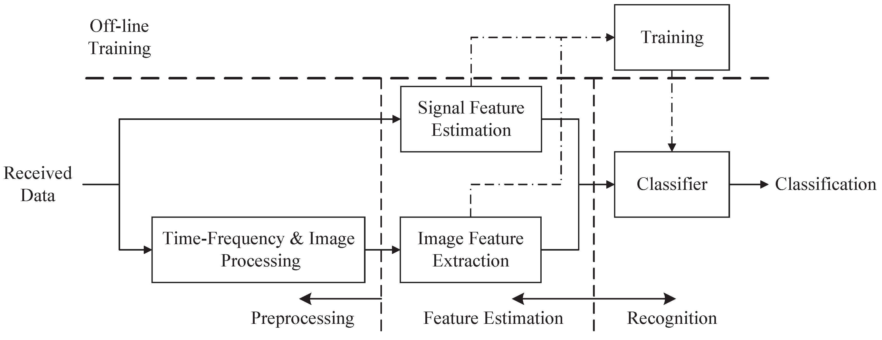
The entire classification system mainly consists of three components: preprocessing, feature estimation and recognition; see Figure 1. It is an automatic process from the preprocessing part to the recognition part. In the preprocessing part, the received data are transformed into time-frequency images by utilizing CWD transformation. Then, the time-frequency images are transformed into the binary image through image binarization, image opening operation and noise-removing algorithms. In the feature extraction part, we extract effective features to train and test the classifier. Different kinds of waveforms have different shapes in the images. After image processing, the differences of shapes are more significant. CNN has a powerful ability of classification, which distinguishes polytime codes from others. To classify these similar waveforms (such as polyphase codes), we extract features from detected signals and binary images. In the recognition part, all of the waveforms are classified via the proposed classifier based on the extracted features.
The hybrid classifier consists of two networks, and ; see Figure 2. The entire classifier can classify 12 different kinds of radar waveforms, which has been mentioned in the writing. is the main network composed of CNN. Its input is a binary image after preprocessing. Additionally, the outputs are five different kinds of classification results. They are four kinds of polytime codes (T1-T4) and others (do not belong to the polytime class). is ENN, which is an auxiliary network. assists the main network in classifying the eight remaining waveforms that do not belong to polytime codes. When the waveform is considered as “others” by , will begin to classify the waveform into one of the eight kinds of waveforms. The proposed structure of the classifier can improve the classified power.
3. Preprocessing
In this section, detected signals are processed into binary images with the Choi–Williams time-frequency distribution.
3.1. Signal Model
We assume the signal is contaminated by additive white Gaussian noise (AWGN). Additionally, the amplitude is constant for time. In summary, the signal model is formulated as follows
where is the n-th sample of complex signals. Additionally, is the n-th sample of complex white Gaussian noise (WGN). The variance of WGN equals . A is the amplitude. However, for the sake of simplicity, we suppose . is the instantaneous phase of complex signals. To process detected signals from real to complex, Hilbert transform is applied [30].
3.2. Choi–Williams Distribution
The Choi–Williams distribution is a kind of time-frequency distribution, which expresses the details of detected signals. It can reduce the cross terms from the signals obviously.
where and t are the axes of frequency and time, respectively. is a two-dimensional low-pass filter to balance cross terms and resolution. The kernel function is formulated as follows:
is the controllable factor. The cross terms will be more obvious with the increase of . In this paper, is applied. In Figure 3, 12 kinds of signals are transformed into time-frequency images through CWD transformation. The work in [31] proposes a new fast calculation of CWD based on standard Fourier transformation (FFT). We could recommend that the number of the sampling is the power of two, such as 256, 512, etc. In this paper, 1024 sampling points are investigated. However, the length of signals is N < 1024 for most of the time. Therefore, zero padding is utilized in the process.
3.3. Binary Image
In this part, the detected signals are processed into binary images with the global thresholding algorithm [32]. Before it is done, we need to resize the time-frequency images to reduce the computational load, in which the resized size is . The algorithm is organized as follows.
- Normalize the resized images , i.e.,
- Estimate the threshold T of , i.e.,
- Separate the image into two pixel groups and ; includes all pixels that values , and includes others;
- Calculate the average value and of two pixel groups and , respectively;
- Update the threshold, i.e.,
- Repeat (b)–(e), until the is smaller than 0.001, i.e.,
- Compute as follows:
- Output .
3.4. Noise Removed
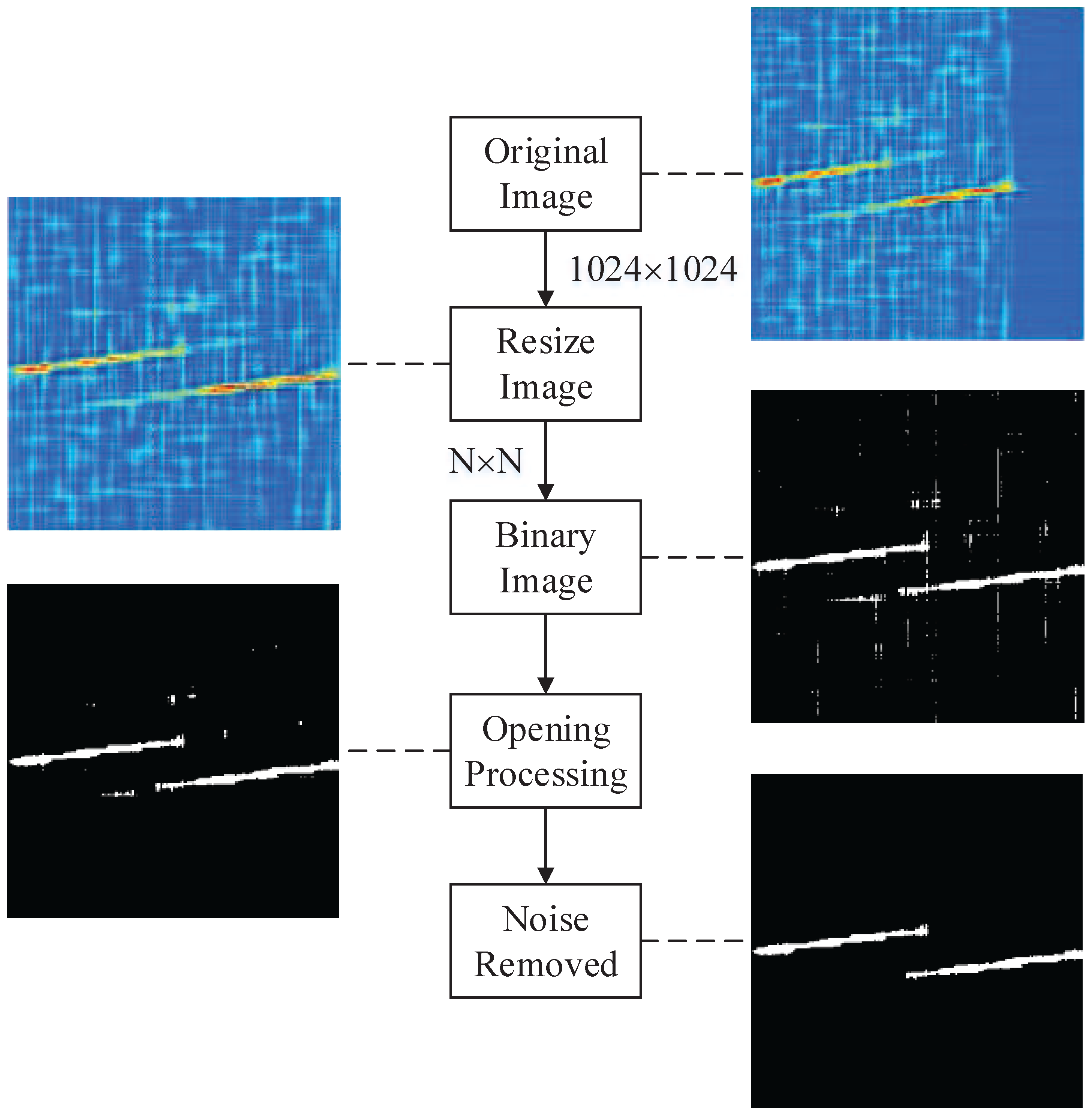
After the operation of binarization, meanwhile, there are some isolated noises and processed noises in . Isolated noises come from the noisy environment. In the binary image, isolated noises are groups of pixels that have no fixed shape. Processed noises are generated from the CWD kernel especially. In the binary image, they are straight lines, long but thin. The length is more than 50 pixels, but the width of lines is less than three pixels. Image opening operation (erosion followed by dilation) algorithms are proposed to remove the processed noises. Additionally, the size of the operational kernel is . It is effective to remove the shape whose width is less than three pixels. For isolated noises, we count the number of pixels of signals or noises. In this paper, the groups are removed, in which sizes are smaller than 10% of the largest one. The content of removing noise is introduced in Figure 4. The finished binary images are used in CNN and feature extraction.
4. Feature Extraction
In this section, we extract some useful features and build a feature vector for ENN in order to assist the CNN to complete recognition. The section consists of two parts, including signal features and image features. The features, which we can estimate or calculate from detected signals directly, belong to signal features. Similarly, image features include the features that are extract from binary images. Table 1 lists the signal features and image features that are used in .
4.1. Signal Features
In this part, the features are extracted from signals based on signal processing approaches.
4.1.1. Based on the Statistics
We estimate the n-order moment of complex signals as follows:
where is the conjugated symbol and N is the sample number. We utilize absolute values to ensure that the estimated values are invariant constants when the signal phase rotates. and are calculated by Equation (4).
4.1.2. Based on the Power Spectral Density
Before estimation of Power Spectral Density (PSD), the detected signals should be normalized as follows:
where is obtained from Equation (4) and is the k-th sample. The variance of additive noise can be obtained in [35].
The PSD are calculated as follows:
where is from Equation (6).
4.1.3. Based on the Instantaneous Properties
Instantaneous properties are the essential characteristics of detected signals. They can distinguish frequency modulated signals from phase modulated signals effectively. In this paper, we estimate the instantaneous frequency and instantaneous phase from samples. The standard deviation of instantaneous phase is addressed in [9]. For brevity, is applied; where, Re and Im are the real and imaginary parts of complex signals, respectively. The standard deviation of instantaneous phase is given by:
where N is the sample number. is the instantaneous phase with the range of .
Instantaneous frequency estimation is more complex than instantaneous phase. We describe the method in several steps to make it clear.
- Calculate ;
- Calculate from ;
- Calculate , i.e.,
- Calculate , i.e.,
- Normalize the instantaneous frequency ,
- Output the standard deviation of instantaneous frequency ,
- ★
- is the unwrapped phase of . When the absolute jumps from , we can add to recover the consecutive phase.
- ★★
- In the sequence of , some spikes are created by processing. We use the median filter algorithm with window size of five to smooth the spikes.
4.2. Image Features
In this part, we extract the features based on binary images. The number of objects () is a key feature. For instance, Costas codes have more than three objects, but Frank code and P2 have two. Additionally, P1, P4 and LFM only have one. We estimate two features and . is the number of objects, the sizes of the pixels of which are more than 20% of the size of the largest object. Likewise,
The maximum energy location in time domain is also a feature, i.e.,
where is the resized time-frequency image and N is the sample number.
The standard deviation of the width of signal objects () can describe the concentration of signal energy. The feature is estimated as follows.
- ●
- Repeat for every object, do ;
- Retain the k-th object and remove others, called ;
- Estimate the principal components of ;
- Rotate the until the principal components are vertical; record as ;
- Sum the vertical axis, i.e.,;
- Normalize as follows
- Estimate the standard deviation of , i.e.,where N is the sample number;
- ●
- Output the rotation degree , which performs Step (c) at the maximum object.
- ●
- Output the average of the , i.e.,
- ★
- Nearest neighbor interpolation is applied in rotation processing.
P2 has a negative slope in five types of polyphase codes. Therefore, the feature can classify P2 from others easily. The feature shows the angle between the maximum object and the vertical direction. It can be obtained from the calculation of easily.
Next, we retain the maximum object in the binary image, but others are removed. The skeleton of the object is extracted by utilizing the image morphology method. Additionally, the linear trend of the object is also estimated based on minimizing the square errors method at the same time. Subtract the linear trend from the skeleton to achieve the difference vector . The standard deviation of is estimated as:
where M is the sample number of .
Some features are extracted by using autocorrelation of , i.e., , . The autocorrelation method makes differences more significant among stepped waveforms (P1, Frank code) and linear waveforms (P3, P4, LFM). See Figure 3 for more details.
The ratio of the maximum value and sidelobe maximum value of is formulated as:
where is the value corresponding to the minimum of and is the value corresponding to the maximum of in the location of .
We estimate the maximum of the absolute of FFT operation as follows:
where is normalized from and .
Pseudo-Zernike moments are invariant for topological transformation [36], such as rotation, translation, mirroring and scaling. They are widely applied in pattern recognition [37,38,39]. The n-order image geometric moments are calculated as:
where is from Section 3.3. The central geometric moments for scale and translation invariant are given by:
where and .
The scale and translation invariant radial geometric moments are shown as:
where and .
Then, the pseudo-Zernike moments can be estimated as follows:
where , and:
At last, is estimated, i.e., . The members of pseudo-Zernike moments include , , , , , and .
5. Classifier
In Section 4, we complete the resized binary image labels for CNN and the feature vector extraction with 22 elements for ENN. In this section, we describe the structure of two networks in detail.
5.1. CNN
CNN is a new neural network, which has a special structure for image feature extraction. Different from traditional network, the input of CNN is a two-dimensional feature (image). The convolution layers can extract information, and pooling layers reduce computer load effectively. CNN is not a full connected network, which is similar to the cerebral cortex. The architecture of the CNN model is shown in Figure 5. CNN has the hierarchical architecture [40]. Hence, we describe the neural architecture as follows.
- The input layer is a binary image, which is from Section 3.4. To reduce the computer load, we resize the image to with the nearest neighbor interpolation algorithm.
- The first hidden layer is a convolutional layer, which has six feature maps. Different feature maps require a different convolutional kernel. has six convolutional kernels with a size of . We utilize to represent the value of the k-th feature map at position in the layer.
- The second hidden layer is a down-sampling layer with six feature maps. In , every feature value is the average of four adjacent elements in . We denote as the context. Further, we have:The size of feature maps in reduces to , compared with feature maps of .
- is a convolutional layer with 16 different kernels. It is not fully connected with the layer [41]. The connection details are described in Table 2. is also utilized to describe the neurons in this layer. For the -th column in Table 2, we mark row indices by For instance, if , then we will get parameters as follows: , , , , Further, the size of the convolutional kernel is . is the -th kernel. Additionally, we have:For example, for the zeroth column, , , , , and we also have:
- Similar to , this layer is a down-sampling layer, called . has 16 feature maps. To follow the context in Equation (20), we donate:
- The connection between and is a full connection. Each kernel in will be connected with all of the feature maps in . There are 120 kernels in this layer. Additionally, the size of the kernel is , which means the output is a column vector with the size of . We describe as the -th feature map of and as the -th kernel. Then, we have:
- Finally, the connected style between and output layer is fully connected. There are five neurons (defined by the classes we want to classify) in the output layer with the function.
5.2. ENN
The three-layer ENN is utilized in the paper for signal classification. The connections, which connect different hidden layers or output layers, have different weights [42]. At every time step, the input is propagated in a feed-forward fashion and the feedback of the output. Additionally, the error back propagation (BP) learning algorithm is also utilized [43]. The connection results in that the context units always maintain a copy of the previous values of hidden units. Thus, the network can keep the past state, which is useful for applications such as sequence prediction [44,45,46]. In Figure 6, there are 46 neurons in the hidden layer. For the input and output layer, the number of neurons is determined by the dimension of input and output vectors. Sigmoid function is proposed in every layer. In [47], Sheela discusses the different methods to fix the neurons number of hidden layers. In this paper, a simple formula is given by:
where X is the dimension of the feature vector. C is the number of categories. The proposed formula cannot determine the optimal number of hidden layer completely. We may fine-tune the number in some situations. Forty-six neurons of hidden layers are applied in this paper.
6. Simulation Results and Discussion
In this section, the performance of the proposed recognition system is analyzed by utilizing simulated data. The section consists of three parts, including creating the simulated data, discussing the relationship between SNR and RSR, depicting the accurate rate of robustness and summarizing the experiments.
6.1. Production of Simulated Signals
In this part, simulated signals are created. In addition, the SNR is proposed as ; where and are the variances of the signal and noise, respectively. Every signal has different parameters that need to be set. We denote a uniform variable based on the sample rate. For example, we assume that the original frequency is 1000 Hz and the sample rate is 8000 Hz. Then, the uniform result is . Meanwhile, expresses the random variable that belongs to . And in this paragraph, also represents a set that includes . Table 3 lists the parameters of the waveforms. For LFM, the sample points change from 500–1000 randomly. Additionally, the range of bandwidth is , so is the initial frequency . For BPSK, the cycle number per phase code and the code periods’ number are and , respectively. The length of the Barker codes is selected from randomly. The carrier frequency is . For the Costas codes, the fundamental frequency is . Additionally, the frequency changed number is . For the Frank code, frequency steps are in the range of . Polyphase codes have the same types of parameters as the Frank code. For polytime codes, the range of segments number and overall code duration are and , respectively.
6.2. Experiment with SNR
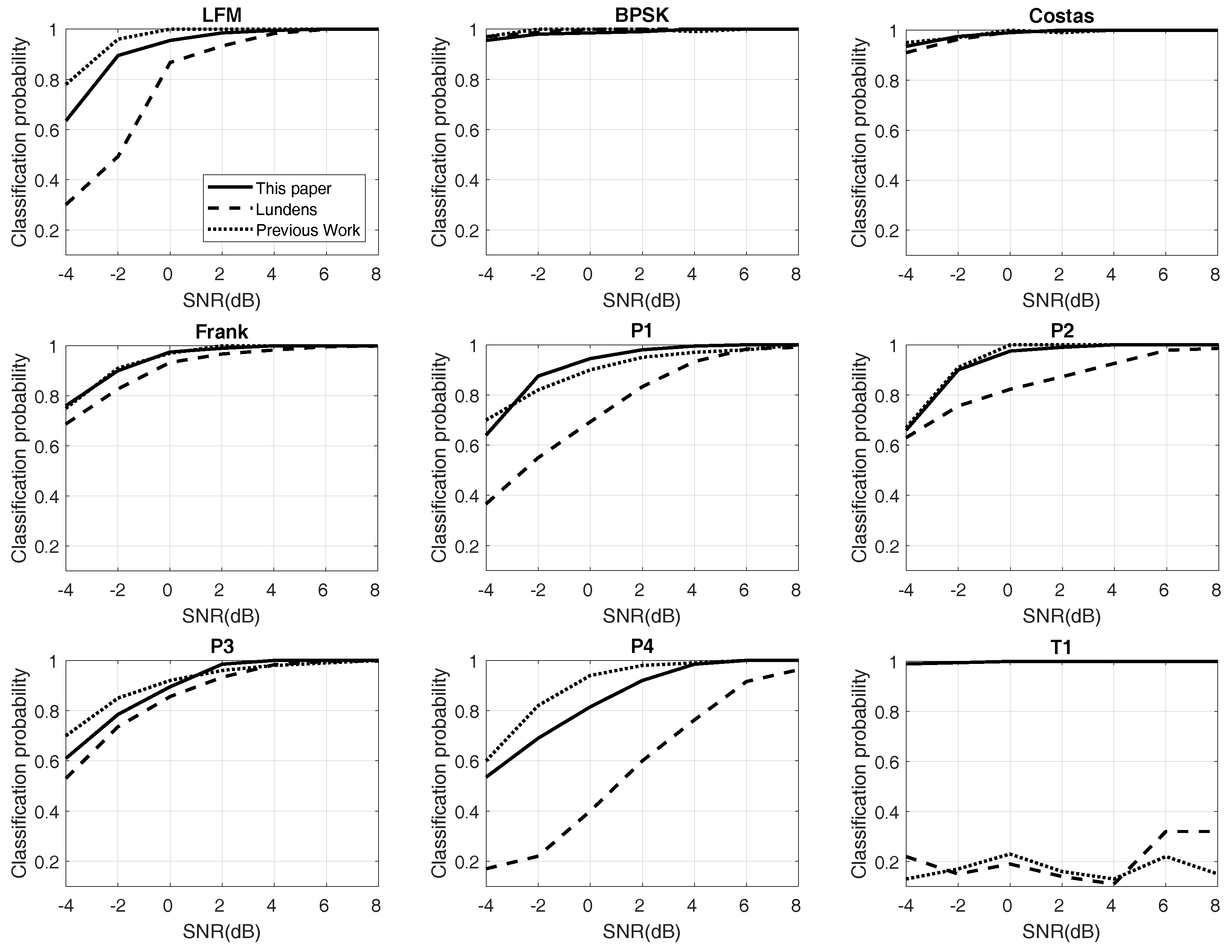
In this part, we depict the relation between SNR and RSR in Figure 7. There are 1000 labels in each waveform class. Twenty percent of the labels are utilized for testing and 80% for training. The result is compared with Lundén’s system [13] and our previous work [14], both of which are wide systems in waveform classification.
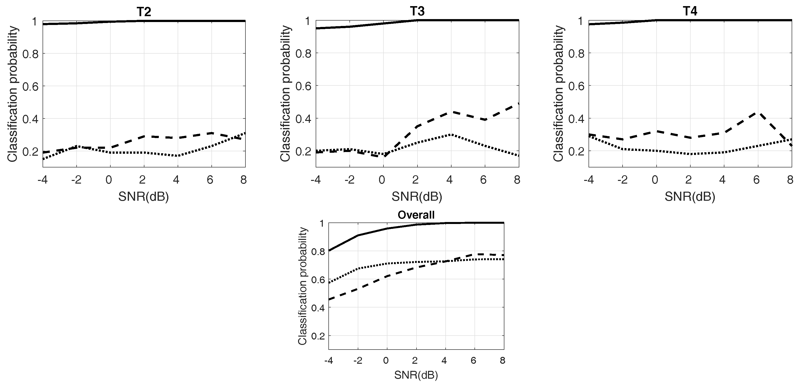
Figure 7 plots the experimental results of RSR with different SNR. Twelve kinds of waveforms and the “overall” are provided. The solid line shows the proposed system, and the dotted lines represent others. For LFM and P4, the proposed approach provides better performance than Lundén’s, especially at low SNR, but poorer than the previous work, although the difference is not too much. For BPSK and Costas codes, the three RSRs almost have similar results, and all of them are at a high level. For Frank and P2, the results of the proposed method and previous work are alike and higher than Lundén’s. In the simulation of P1, the proposed method is the best when the SNR is more than −2 dB. The results of P3 are similar to P1; proposed method performs well at high SNR. For polytime codes, the proposed approach also has excellent RSRs. It benefits from the outstanding design of pre-processing and the high RSR of the classifier. Finally, the overall RSR has been raised by 20% in the proposed approaches, compared to Lundén’s and previous work. At SNR of −2 dB, the overall probabilities are still more than 90%. Table 4 exhibits the confusion table of 12 kinds of waveforms at the SNR of −2 dB. As Table 4 shows, the waveforms of P3 and P4 are not “always” classified correctly. For P3, most of the errors are classified into the Frank code. Meanwhile, most of the errors of P4 are classified into LFM. However, the two pairs are very similar; see Figure 3.
6.3. Experiment with Robustness
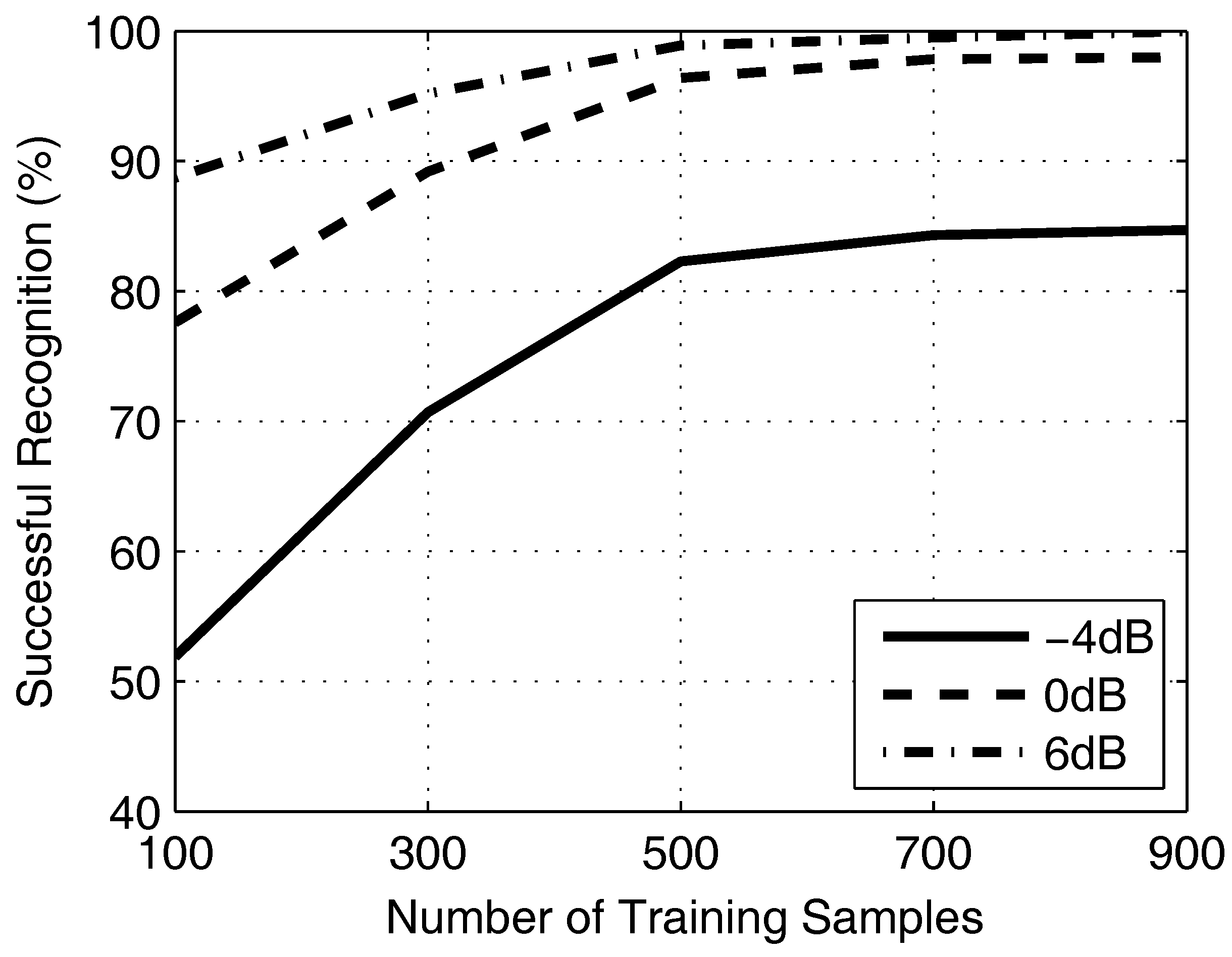
The robustness of proposed approaches is explored in different training samples. There are 900 label samples in each waveform for training and 100 labels for testing. Afterwards, the training samples will be increased from 100–900 with a step of 200. Meanwhile, the experiment will be repeated for three times in the condition of SNR = −4 dB, 0 dB and 6 dB.
Figure 8 plots the impact of training samples on successful recognition with three conditions of SNR. In general, it is positively correlated between training samples and successful recognition. When the samples are less than 500, the successful recognition increases obviously. However, when the samples are more than 500, the successful recognition is substantially retained. It means that the proposed approaches are able to work well in a small number of samples.
6.4. Experiment with Computational Burden
Computational burden is also an important issue for the classification system. We measure the time of the proposed method and compare it with [13,14] in the same conditions. Three different SNRs, −4 dB, −0 dB and 6 dB are tested, and each test repeats 50 times to calculate the average value. Table 5 shows the testing environment, and Table 6 demonstrates the testing results, respectively.
In Table 6, the proposed method and previous work spend less than 60 s, while Lundén’s more than 80 s; because Lundén’s method has more calculations, we do not need to compute, such as the Wigner–Ville distribution, peak search and data driven, etc. We also improve the effectiveness of the system and reduce the consumption of time compared with previous work. In the same type of waveform, the highest SNR has the least time. In the different types of waveforms, BPSK is easiest to calculate, but P3 code is the opposite. However, overall, the change of cost is not obvious. The proposed method is stable, and different waveforms or SNR also have little effect on the computational burden of the classification system.
7. Conclusions
In this paper, an automatic system to realize the recognition of radar signal waveforms is proposed. We build the processing flow for detected signals by utilizing signal and image processing algorithms. Using these methods, the signal waveforms are fully represented via sets of feature vectors and binary images. The vectors and images are classified into 12 types in the classifier. The simulation results show that the overall RSR is more than 94% at SNR ≥−2 dB. Additionally, the processes of feature extraction and noise removed make the system robust. When the sample labels are more than 500, the successful recognition is substantially retained. At last, the computational burden is tested. The proposed method is stable in different waveforms or SNR and spends less time than Lundén’s method and our previous work.
Acknowledgments
This work was supported by the National Natural Science Foundation of China (NSFC) under Grants 61201410, 61571149 and the Fundamental Research Funds for the Central Universities HEUCF170802. The authors would like to thank the associate editor and reviewers for useful feedback.
Author Contributions
M.Z. and M.D. conceived of and designed the experiments. M.Z. performed the experiments. M.Z. and LT.L. analyzed the data. LP.G. contributed analysis tools. M.Z. wrote the paper.
Conflicts of Interest
All co-authors have seen and agree with the contents of the manuscript and declare no conflict of interest. We certify that the submission is original work and is not under review at any other publication. The founding sponsors have no role in the design of the study; in the collection, analyses or interpretation of data; in the writing of the manuscript; nor in the decision to publish the results.
Abbreviations
The following abbreviations are used in this manuscript:
| LPI | Low probability of intercept |
| EW | Electronic warfare |
| ELINT | Electronic intelligence |
| PSK | Phase shift keying |
| FSK | Frequency shift keying |
| ASK | Smplitude shift keying |
| PRI | Pulse repetition interval |
| PW | Pulse width |
| RSR | Ratio of successful recognition |
| SNR | Signal to noise ratio |
| MLP | Multi-layer perceptron |
| AD | Atomic decomposition |
| LFM | Linear frequency modulation |
| CW | Continuous wave |
| STFT | Short time Fourier transform |
| SC | Sparse classification |
| CNN | Convolutional neural network |
| DNN | Deep neural network |
| SVM | Support vector machine |
| BPSK | Binary phase shift keying |
| ENN | Elman neural network |
| CWD | Choi–Williams time-frequency distribution |
| PCA | Principal component analysis |
| AWGN | Additive white Gaussian noise |
| WGN | White gaussian noise |
| FFT | Fast Fourier transformation |
| PSD | Power spectral density |
| CPU | Central Processing Unit |
| GPU | Graphics Processing Unit |
References
- Adamy, D.L. EW 102: A Second Course in Electronic Warfare; Artech House: Norwood, MA, USA, 2004. [Google Scholar]
- Adamy, D.L. EW 101: A First Course in Electronic Warfare; Artech House: Norwood, MA, USA, 2000. [Google Scholar]
- Nandi, A.; Azzouz, E. Automatic analogue modulation recognition. Signal Process. 1995, 46, 211–222. [Google Scholar] [CrossRef]
- Dudczyk, J.; Kawalec, A. Specific emitter identification based on graphical representation of the distribution of radar signal parameters. Bull. Pol. Acad. Sci. Tech. Sci. 2015, 63, 391–396. [Google Scholar] [CrossRef]
- Dudczyk, J.; Kawalec, A. Fast-decision identification algorithm of emission source pattern in database. Bull. Pol. Acad. Sci. Tech. Sci. 2015, 63, 385–389. [Google Scholar] [CrossRef]
- Dudczyk, J. A method of feature selection in the aspect of specific identification of radar signals. Bull. Pol. Acad. Sci. Tech. Sci. 2017, 65, 113–119. [Google Scholar] [CrossRef]
- Dudczyk, J. Radar Emission Sources Identification Based on Hierarchical Agglomerative Clustering for Large Data Sets. J. Sens. 2016, 2016, 1879327. [Google Scholar] [CrossRef]
- Nandi, A.K.; Azzouz, E.E. Algorithms for automatic modulation recognition of communication signals. IEEE Trans. Commun. 1998, 46, 431–436. [Google Scholar] [CrossRef]
- Wong, M.D.; Nandi, A.K. Automatic digital modulation recognition using artificial neural network and genetic algorithm. Signal Process. 2004, 84, 351–365. [Google Scholar] [CrossRef]
- López-Risueño, G.; Grajal, J.; Sanz-Osorio, Á. Digital channelized receiver based on time-frequency analysis for signal interception. IEEE Trans. Aerosp. Electron. Syst. 2005, 41, 879–898. [Google Scholar] [CrossRef]
- Cohen, L. Time-frequency distributions-a review. Proc. IEEE 1989, 77, 941–981. [Google Scholar] [CrossRef]
- Lopez-Risueno, G.; Grajal, J.; Yeste-Ojeda, O. Atomic decomposition-based radar complex signal interception. IEE Proc. Radar Sonar Navig. 2003, 150, 323–331. [Google Scholar] [CrossRef]
- Lundén, J.; Koivunen, V. Automatic radar waveform recognition. IEEE J. Sel. Top. Signal Process. 2007, 1, 124–136. [Google Scholar] [CrossRef]
- Ming, Z.; Lutao, L.; Ming, D. LPI Radar Waveform Recognition Based on Time-Frequency Distribution. Sensors 2016, 16, 1682. [Google Scholar] [CrossRef]
- Ma, J.; Huang, G.; Zuo, W.; Wu, X.; Gao, J. Robust radar waveform recognition algorithm based on random projections and sparse classification. IET Radar Sonar Navig. 2013, 8, 290–296. [Google Scholar] [CrossRef]
- Lawrence, S.; Giles, C.L.; Tsoi, A.C.; Back, A.D. Face recognition: A convolutional neural-network approach. IEEE Trans. Neural Netw. 1997, 8, 98–113. [Google Scholar] [CrossRef] [PubMed]
- LeCun, Y.; Huang, F.J.; Bottou, L. Learning methods for generic object recognition with invariance to pose and lighting. In Proceedings of the 2004 IEEE Computer Society Conference on Computer Vision and Pattern Recognition, Washington, DC, USA, 27 June–2 July 2004. [Google Scholar]
- Sainath, T.N.; Kingsbury, B.; Saon, G.; Soltau, H.; Mohamed, A.R.; Dahl, G.; Ramabhadran, B. Deep convolutional neural networks for large-scale speech tasks. Neural Netw. 2015, 64, 39–48. [Google Scholar] [CrossRef] [PubMed]
- Yoshioka, T.; Karita, S.; Nakatani, T. Far-field speech recognition using CNN-DNN-HMM with convolution in time. In Proceedings of the IEEE International Conference on Acoustics, Speech and Signal Processing (ICASSP), Brisbane, QLD, Australia, 19–24 April 2015; pp. 4360–4364. [Google Scholar]
- Swietojanski, P.; Arnab, G.; Steve, R. Convolutional neural networks for distant speech recognition. IEEE Signal Process. Lett. 2014, 21, 1120–1124. [Google Scholar]
- Abdel-Hamid, O.; Mohamed, A.R.; Jiang, H.; Penn, G. Applying convolutional neural networks concepts to hybrid NN-HMM model for speech recognition. In Proceedings of the Acoustics, Speech and Signal Processing (ICASSP), 2012 IEEE International Conference on Acoustics, Speech and Signal Processing (ICASSP), Kyoto, Japan, 25–30 March 2012; pp. 4277–4280. [Google Scholar]
- Lin, T.Y.; RoyChowdhury, A.; Maji, S. Bilinear CNN models for fine-grained visual recognition. In Proceedings of the IEEE International Conference on Computer Vision, Cambridge, MA, USA, 20–23 June 2015; pp. 1449–1457. [Google Scholar]
- Vaddi, R.S.; Boggavarapu, L.N.P.; Vankayalapati, H.D.; Anne, K.R. Comparative analysis of contrast enhancement techniques between histogram equalization and CNN. In Proceedings of the 2011 Third International Conference on Advanced Computing, Chennai, India, 14–16 December 2011; pp. 106–110. [Google Scholar]
- Zhou, M.K.; Zhang, X.Y.; Yin, F.; Liu, C.L. Discriminative quadratic feature learning for handwritten Chinese character recognition. Pattern Recognit. 2016, 49, 7–18. [Google Scholar] [CrossRef]
- Akhand, M.A.H.; Rahman, M.M.; Shill, P.C.; Islam, S.; Rahman, M.H. Bangla handwritten numeral recognition using convolutional neural network. In Proceedings of the 2015 International Conference on Electrical Engineering and Information Communication Technology (ICEEICT), Dhaka, Bangladesh, 21–23 May 2015; pp. 1–5. [Google Scholar]
- Niu, X.X.; Suen, C.Y. A novel hybrid CNN–SVM classifier for recognizing handwritten digits. Pattern Recognit. 2012, 45, 1318–1325. [Google Scholar] [CrossRef]
- Abdel-Hamid, O.; Mohamed, A.R.; Jiang, H.; Deng, L.; Penn, G.; Yu, D. Convolutional neural networks for speech recognition. IEEE/ACM Trans. Audio Speech Lang. Process. 2014, 22, 1533–1545. [Google Scholar] [CrossRef]
- Feng, Z.; Liang, M.; Chu, F. Recent advances in time–frequency analysis methods for machinery fault diagnosis: A review with application examples. Mech. Syst. Signal Process. 2013, 38, 165–205. [Google Scholar] [CrossRef]
- Chen, B.; Shu, H.; Zhang, H.; Chen, G.; Toumoulin, C.; Dillenseger, J.L.; Luo, L.M. Quaternion Zernike moments and their invariants for color image analysis and object recognition. Signal Process. 2012, 92, 308–318. [Google Scholar] [CrossRef]
- Xu, B.; Sun, L.; Xu, L.; Xu, G. Improvement of the Hilbert method via ESPRIT for detecting rotor fault in induction motors at low slip. IEEE Trans. Energy Convers. 2013, 28, 225–233. [Google Scholar] [CrossRef]
- Pace, P.E. Detecting and Classifying Low Probability of Intercept Radar, 2nd ed.; Artech House: Norwood, MA, USA, 2009. [Google Scholar]
- Gonzalez, R.C. Digital Image Processing; Pearson Education: Delhi, India, 2009. [Google Scholar]
- Zhu, Z.; Aslam, M.W.; Nandi, A.K. Genetic algorithm optimized distribution sampling test for M-QAM modulation classification. Signal Process. 2014, 94, 264–277. [Google Scholar] [CrossRef]
- Ozen, A.; Ozturk, C. A novel modulation recognition technique based on artificial bee colony algorithm in the presence of multipath fading channels. In Proceedings of the 2013 36th International Conference on Telecommunications and Signal Processing (TSP), Rome, Italy, 2–4 July 2013; pp. 239–243. [Google Scholar]
- Stoica, P.; Moses, R.L. Spectral Analysis of Signals; Pearson/Prentice Hall Upper: Saddle River, NJ, USA, 2005. [Google Scholar]
- Bailey, R.R.; Srinath, M. Orthogonal moment features for use with parametric and non-parametric classifiers. IEEE Trans. Pattern Anal. Mach. Intell. 1996, 18, 389–399. [Google Scholar] [CrossRef]
- Chen, Z.; Sun, S.K. A Zernike moment phase-based descriptor for local image representation and matching. IEEE Trans. Image Process. 2010, 19, 205–219. [Google Scholar] [CrossRef] [PubMed]
- Tan, C.W.; Kumar, A. Accurate iris recognition at a distance using stabilized iris encoding and Zernike moments phase features. IEEE Trans. Image Process. 2014, 23, 3962–3974. [Google Scholar] [CrossRef] [PubMed]
- Honarvar, B.; Paramesran, R.; Lim, C.L. Image reconstruction from a complete set of geometric and complex moments. Signal Process. 2014, 98, 224–232. [Google Scholar] [CrossRef]
- Lauer, F.; Suen, C.Y.; Bloch, G. A trainable feature extractor for handwritten digit recognition. Pattern Recognit. 2007, 40, 1816–1824. [Google Scholar] [CrossRef]
- LeCun, Y.; Bottou, L.; Bengio, Y.; Haffner, P. Gradient-based learning applied to document recognition. Proc. IEEE 1998, 86, 2278–2324. [Google Scholar] [CrossRef]
- Johnson, A.E.; Ghassemi, M.M.; Nemati, S.; Niehaus, K.E.; Clifton, D.; Clifford, G.D. Machine learning and decision support in critical care. Proc. IEEE 2016, 104, 444–466. [Google Scholar] [CrossRef] [PubMed]
- Bengio, Y.; Courville, A.; Vincent, P. Representation learning: A review and new perspectives. IEEE Trans. Pattern Anal. Mach. Intell. 2013, 35, 1798–1828. [Google Scholar] [CrossRef] [PubMed]
- Lin, W.M.; Hong, C.M.; Chen, C.H. Neural-network-based MPPT control of a stand-alone hybrid power generation system. IEEE Trans. Power Electron. 2011, 26, 3571–3581. [Google Scholar] [CrossRef]
- Lin, C.M.; Boldbaatar, E.-A. Autolanding control using recurrent wavelet Elman neural network. IEEE Trans. Syst. Man Cybern.-Syst. 2015, 45, 1281–1291. [Google Scholar] [CrossRef]
- Yin, S.; Yang, H.; Gao, H.; Qiu, J.; Kaynak, O. An adaptive NN-based approach for fault-tolerant control of nonlinear time-varying delay systems with unmodeled dynamics. IEEE Trans. Neural Netw. Learn. Syst. 2016, PP, 1–12. [Google Scholar] [CrossRef] [PubMed]
- Sheela, K.G.; Deepa, S. Review on methods to fix number of hidden neurons in neural networks. Math. Probl. Eng. 2013, 2013, 425740. [Google Scholar] [CrossRef]
Figure 1.
The figure shows the systematic components. Received data is processed in the preprocessing part and feature estimation part to extract features. And the data is classified in the classifier part.
Figure 1.
The figure shows the systematic components. Received data is processed in the preprocessing part and feature estimation part to extract features. And the data is classified in the classifier part.

Figure 2.
This figure shows the details of the classifier. is the main network composed of CNN and is ENN. assists the main network to complete the classification.
Figure 2.
This figure shows the details of the classifier. is the main network composed of CNN and is ENN. assists the main network to complete the classification.
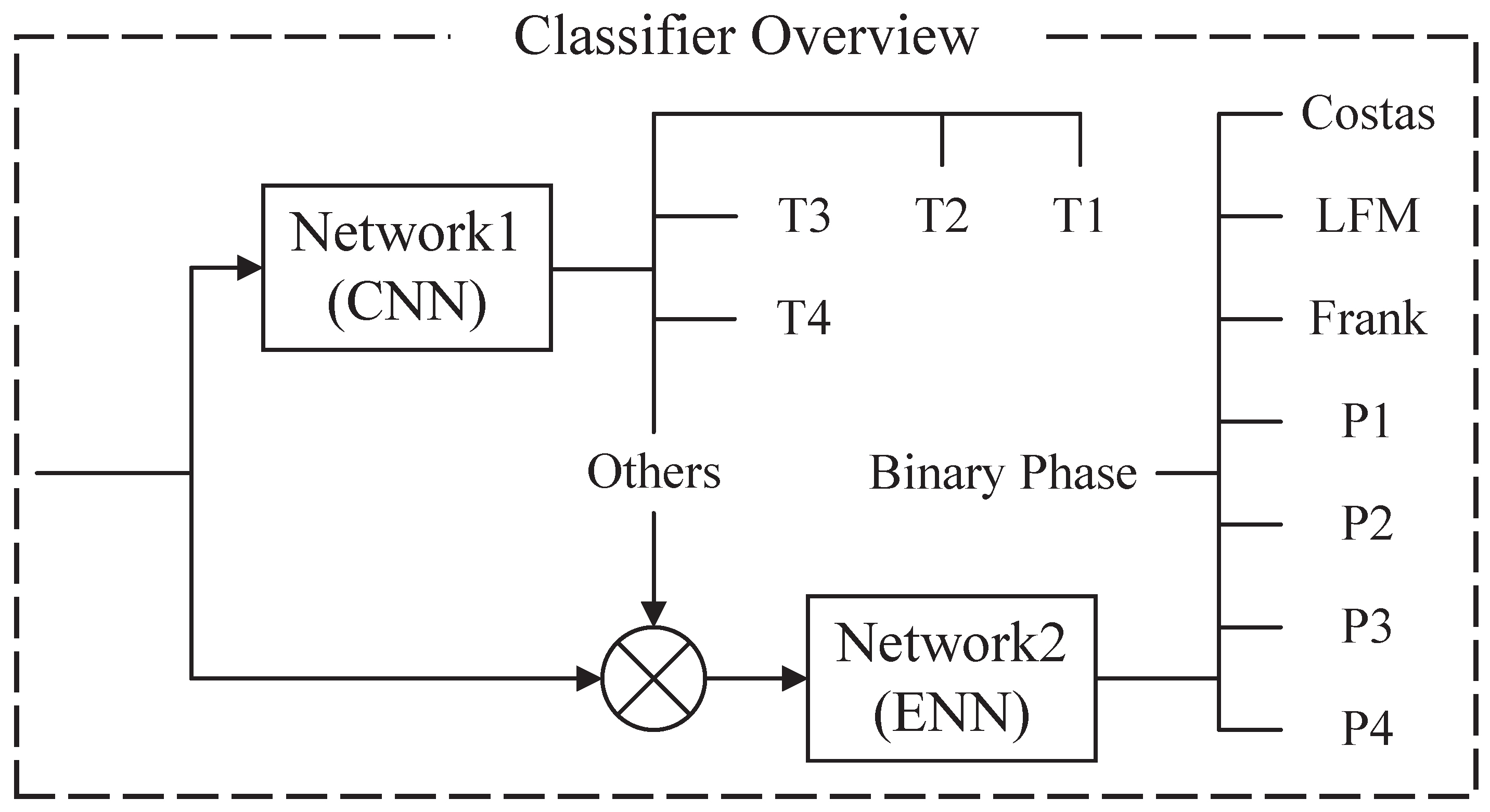
Figure 3.
In this figure, different waveform classes are shown, including Linear Frequency Modulation (LFM), Binray Phase Shift Keying (BPSK), Frank, Costas codes, P1-P4 codes and T1-T4 codes. There are significant differences among the Choi-Williams Time-Frequency Distribution (CWD) images.
Figure 3.
In this figure, different waveform classes are shown, including Linear Frequency Modulation (LFM), Binray Phase Shift Keying (BPSK), Frank, Costas codes, P1-P4 codes and T1-T4 codes. There are significant differences among the Choi-Williams Time-Frequency Distribution (CWD) images.
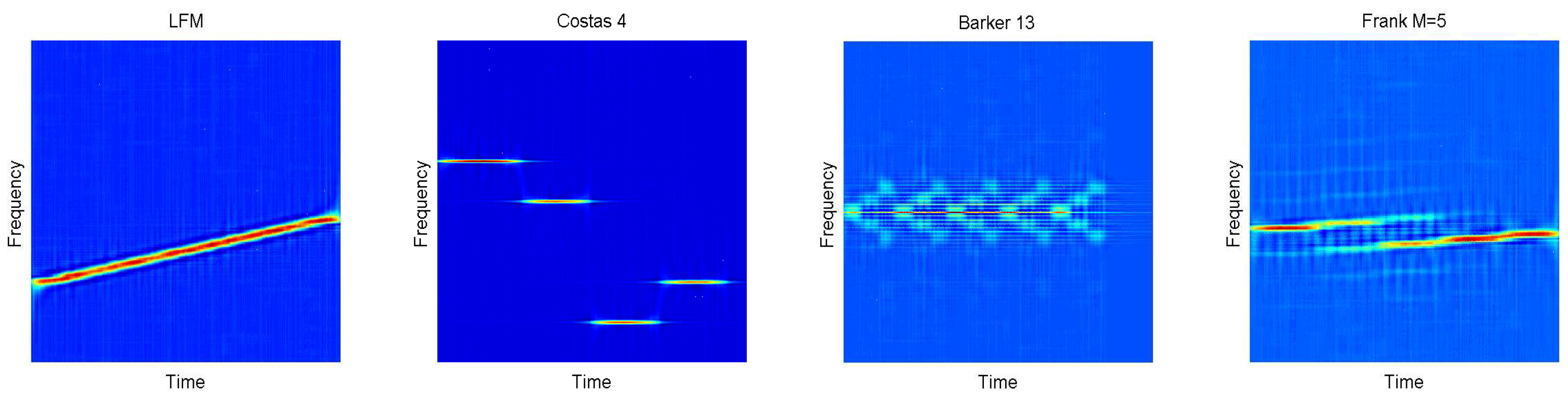
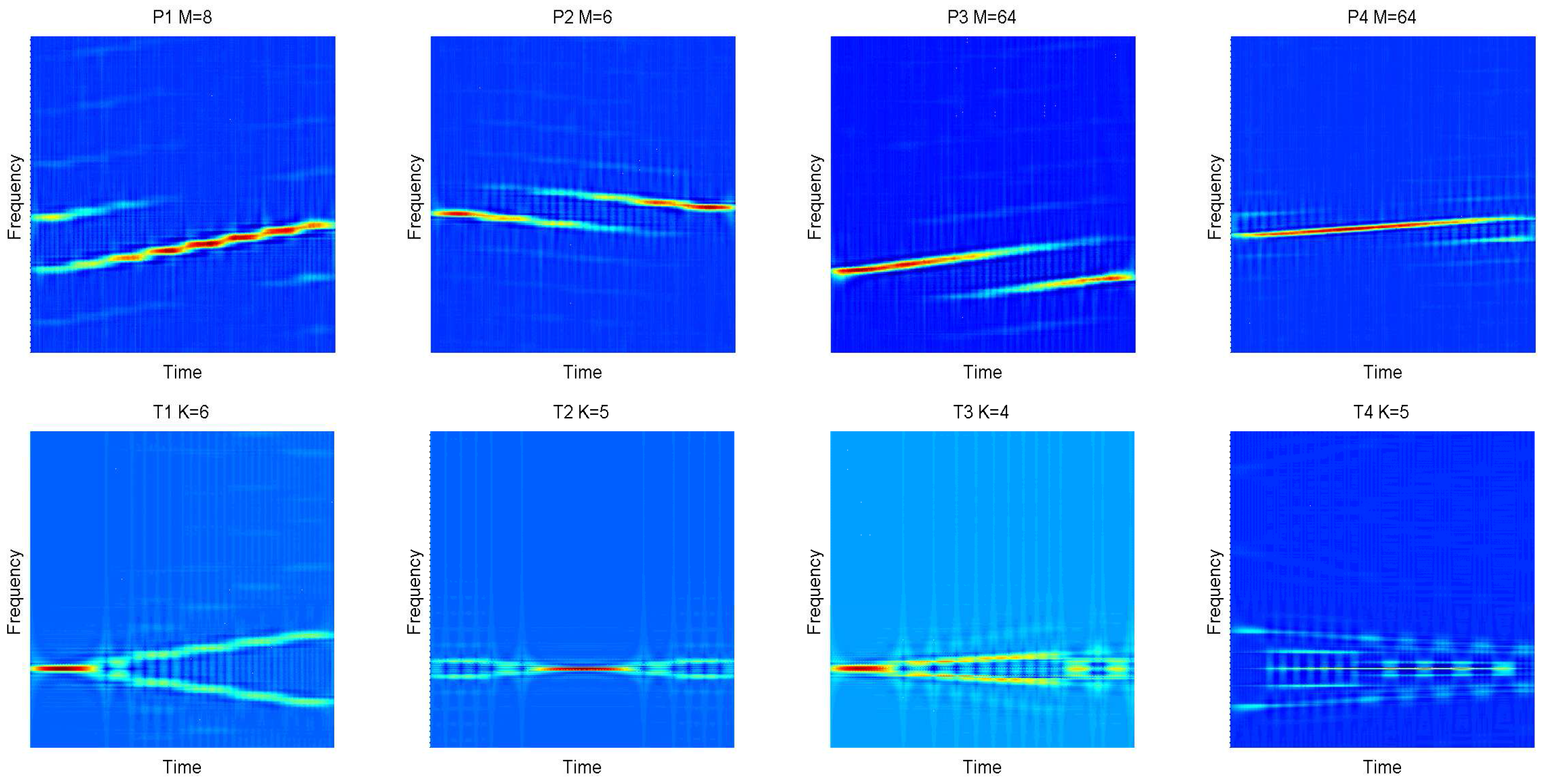
Figure 4.
In this figure, we exhibit the processing with P3 code at an signal-to-noise ratio (SNR) of −4 dB.
Figure 4.
In this figure, we exhibit the processing with P3 code at an signal-to-noise ratio (SNR) of −4 dB.

Figure 5.
The figure shows the structure of Convolutional Neural Network (CNN). The input image are processed in the hidden layers and classified in the out layer.
Figure 5.
The figure shows the structure of Convolutional Neural Network (CNN). The input image are processed in the hidden layers and classified in the out layer.
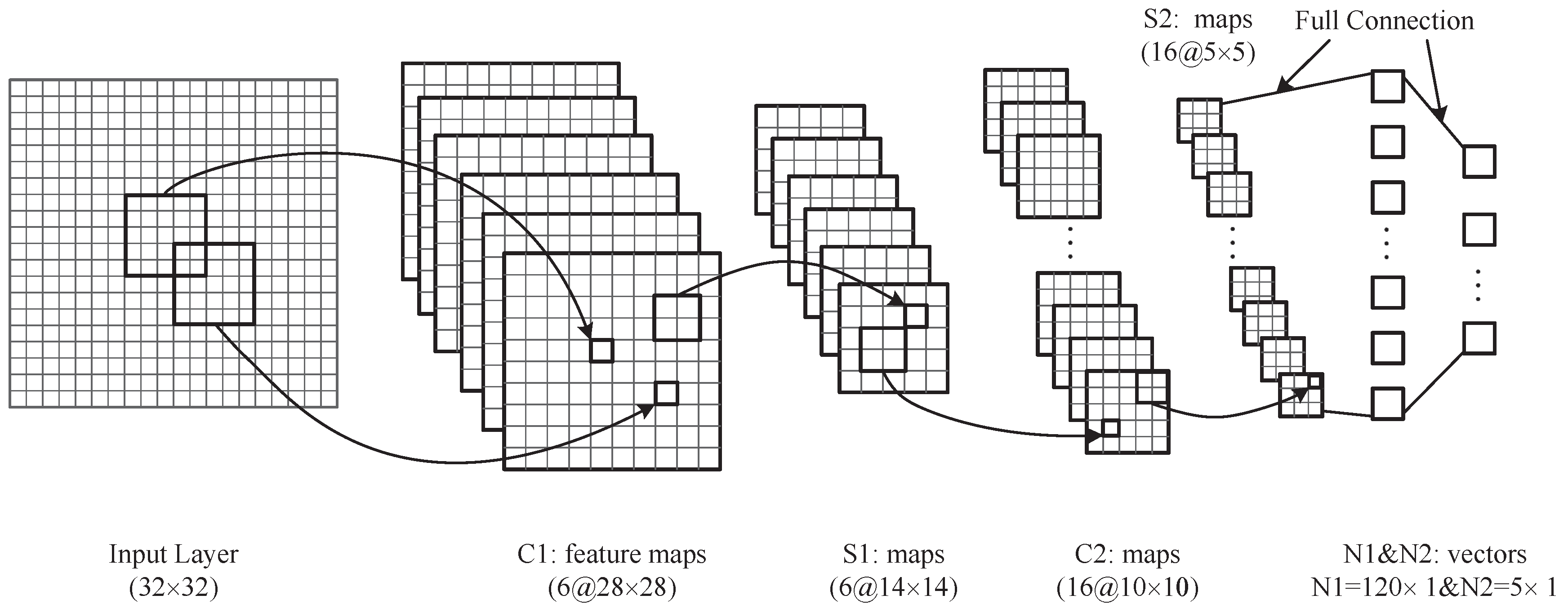
Figure 6.
This figure shows the structure of Elman neural network. It is a 3 layers network that has feedback loops. So, the network can keep the past state, which is useful for waveform classification.
Figure 6.
This figure shows the structure of Elman neural network. It is a 3 layers network that has feedback loops. So, the network can keep the past state, which is useful for waveform classification.
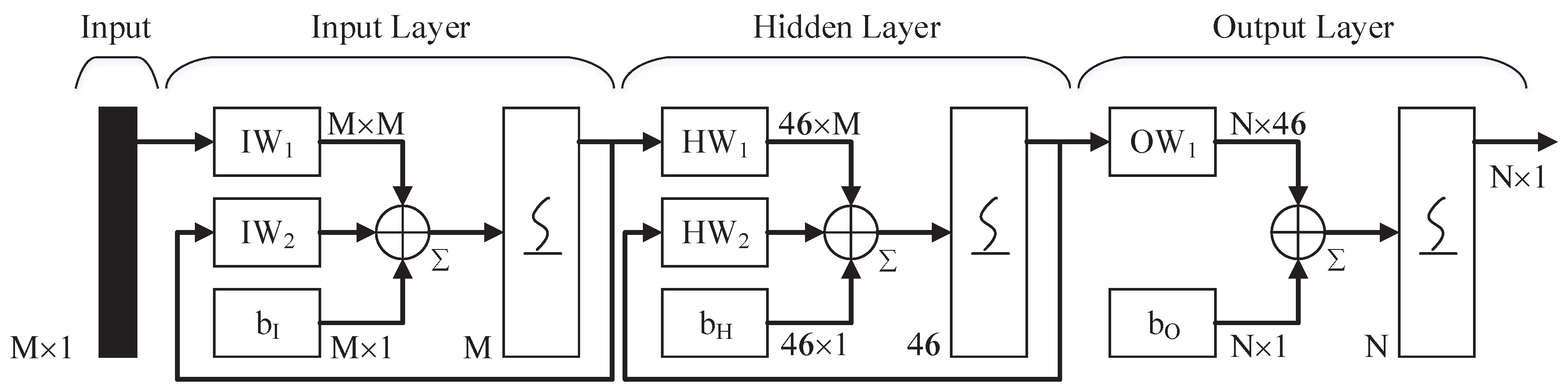
Figure 7.
This figure depicts the different probabilities of 12 types of radar waveforms with testing data. SNR: Signal-to-noise ratio.
Figure 7.
This figure depicts the different probabilities of 12 types of radar waveforms with testing data. SNR: Signal-to-noise ratio.


Figure 8.
The figure shows the successful recognition ratio of different numbers of samples.

Table 1.
List of the features for
| Index | Description | Symbol |
|---|---|---|
| 1 | Moment (1-order) | |
| 2 | Moment (2-order) | |
| 3 | Cumulant (2-order) | |
| 4 | PSD maximum (1-order) | |
| 5 | PSD maximum (2-order) | |
| 6 | Std. of phase | |
| 7 | Std. of frequency | |
| 8 | No. of objects (20%) | |
| 9 | No. of objects (50%) | |
| 10 | CWD time peak location | |
| 11 | Std. of object width | |
| 12 | Maximum of PCA degree | |
| 13 | Std. of | |
| 14 | Autocorrelationof | r |
| 15 | FFT of correlation | |
| 16 | Pseudo-Zernike moment (2-order) | |
| 17 | Pseudo-Zernike moment (3-order) | |
| 18 | Pseudo-Zernike moment (4-order) | |
| 19 | Pseudo-Zernike moment (4-order) | |
| 20 | Pseudo-Zernike moment (5-order) | |
| 21 | Pseudo-Zernike moment (6-order) | |
| 22 | Pseudo-Zernike moment (7-order) |
PSD: Power Spectral Density. PCA: Principal Component Analysis. FFT: Fast Fourier Transformation. Std.: Standard Deviation.
Table 2.
Connection detail about and .
| 0 | 1 | 2 | 3 | 4 | 5 | 6 | 7 | 8 | 9 | 10 | 11 | 12 | 13 | 14 | 15 | |
|---|---|---|---|---|---|---|---|---|---|---|---|---|---|---|---|---|
| 0 | ✔ | ✔ | ✔ | ✔ | ✔ | ✔ | ✔ | ✔ | ✔ | ✔ | ||||||
| 1 | ✔ | ✔ | ✔ | ✔ | ✔ | ✔ | ✔ | ✔ | ✔ | ✔ | ||||||
| 2 | ✔ | ✔ | ✔ | ✔ | ✔ | ✔ | ✔ | ✔ | ✔ | ✔ | ||||||
| 3 | ✔ | ✔ | ✔ | ✔ | ✔ | ✔ | ✔ | ✔ | ✔ | ✔ | ||||||
| 4 | ✔ | ✔ | ✔ | ✔ | ✔ | ✔ | ✔ | ✔ | ✔ | ✔ | ||||||
| 5 | ✔ | ✔ | ✔ | ✔ | ✔ | ✔ | ✔ | ✔ | ✔ | ✔ |
Table 3.
List of the parameters of simulated signals.
| Signal Waveforms | Parameters | Uniform Ranges |
|---|---|---|
| - | Sampling rate | |
| LFM | Samples number | |
| Bandwidth | ||
| Initial frequency | ||
| BPSK | Cycles per phase code | |
| Number of code periods | ||
| Barker codes | ||
| Carrier frequency | ||
| Costas codes | N | |
| Fundamental frequency | ||
| Number changed | ||
| Frank and P1 codes | ||
| Frequency steps | ||
| P2 code | ||
| M | ||
| P3 and P4 codes | ||
| M | ||
| T1-T4 codes | Number of segments | |
| Overall code duration |
Table 4.
Confusion matrix for the system at an SNR of dB. The overall Ratio of Successful Recognition (RSR) is 94.5%.
Table 4.
Confusion matrix for the system at an SNR of dB. The overall Ratio of Successful Recognition (RSR) is 94.5%.
| T1 | T2 | T3 | T4 | LFM | Costas | BPSK | Frank | P1 | P2 | P3 | P4 | |
|---|---|---|---|---|---|---|---|---|---|---|---|---|
| T1 | 99.5 | 0 | 0 | 0 | 0 | 0 | 0 | 0 | 0 | 0 | 0 | 0 |
| T2 | 0 | 98.5 | 0 | 0 | 0 | 0 | 0 | 0 | 0 | 0 | 0 | 0 |
| T3 | 0.5 | 0 | 96 | 0 | 0 | 0 | 0 | 0 | 0 | 0 | 0 | 0 |
| T4 | 0 | 0 | 0 | 98.5 | 0 | 1.5 | 2 | 0 | 0 | 0 | 0 | 0 |
| LFM | 0 | 0 | 0 | 0 | 89.5 | 0 | 0 | 0 | 1 | 0 | 2 | 15.5 |
| Costas | 0 | 0 | 0 | 0 | 0 | 97.5 | 0 | 0 | 0 | 1.5 | 1 | 0 |
| BPSK | 0 | 0 | 0.5 | 0 | 0 | 0 | 98 | 1 | 0 | 0 | 0 | 0.5 |
| Frank | 0 | 0 | 0 | 0 | 1 | 1 | 0 | 90 | 4 | 7 | 11 | 1.5 |
| P1 | 0 | 0 | 0 | 0 | 0.5 | 0 | 0 | 0 | 87.5 | 0 | 0 | 7.5 |
| P2 | 0 | 0 | 0 | 0 | 1 | 0 | 0 | 6.5 | 5.5 | 90 | 3 | 5.5 |
| P3 | 0 | 1.5 | 3.5 | 1.5 | 0 | 0 | 0 | 2.5 | 1 | 1.5 | 78.5 | 0.5 |
| P4 | 0 | 0 | 0 | 0 | 8 | 0 | 0 | 0 | 1 | 0 | 4.5 | 69 |
Table 5.
The testing environment.
| Item | Model/Version |
|---|---|
| CPU | E5-1620v2 (Intel) |
| Memory | 16GB (DDR3 @ 1600 MHz) |
| GPU | NVS315 (Quadro) |
| MATLAB | R2012a |
CPU: Central Processing Unit. GPU: Graphics Processing Unit. MATLAB is a software produced by the MathWorks, Inc. that located in Natick, Massachusetts, United States.
Table 6.
Computational burden test (this paper/previous work/Lundén; unit: s).
| LFM | BPSK | Costas | Frank | |
|---|---|---|---|---|
| −4 dB | 54.798/55.302/85.331 | 51.117/51.132/82.553 | 54.463/54.798/84.735 | 56.115/56.221/86.132 |
| 0 dB | 54.336/55.096/85.152 | 50.860/50.903/82.094 | 54.108/54.255/84.113 | 55.704/55.909/85.754 |
| 6 dB | 53.983/54.887/84.755 | 50.378/50.875/81.598 | 53.766/53.842/83.795 | 55.368/55.806/85.389 |
| P1 | P2 | P3 | P4 | |
| −4 dB | 58.887/58.889/88.112 | 55.559/55.759/86.739 | 58.386/58.522/87.117 | 54.105/54.732/85.079 |
| 0 dB | 58.398/58.519/87.847 | 55.308/55.431/86.180 | 58.106/58.310/86.869 | 53.858/54.338/84.787 |
| 6 dB | 57.792/58.034/87.106 | 54.668/55.307/85.848 | 57.707/57.802/86.478 | 53.501/54.196/84.503 |
| T1 | T2 | T3 | T4 | |
| −4 dB | 53.781/54.086/83.308 | 52.896/53.117/85.401 | 55.269/55.887/86.249 | 56.703/56.861/85.322 |
| 0 dB | 53.266/53.799/83.011 | 52.715/52.980/85.166 | 54.523/55.300/86.093 | 56.359/56.622/85.054 |
| 6 dB | 52.823/53.201/82.799 | 52.107/52.741/84.455 | 54.396/54.916/85.702 | 55.993/56.279/84.811 |
© 2017 by the authors. Licensee MDPI, Basel, Switzerland. This article is an open access article distributed under the terms and conditions of the Creative Commons Attribution (CC BY) license (http://creativecommons.org/licenses/by/4.0/).
Share and Cite
MDPI and ACS Style
Zhang, M.; Diao, M.; Gao, L.; Liu, L. Neural Networks for Radar Waveform Recognition. Symmetry 2017, 9, 75. https://doi.org/10.3390/sym9050075
AMA Style
Zhang M, Diao M, Gao L, Liu L. Neural Networks for Radar Waveform Recognition. Symmetry. 2017; 9(5):75. https://doi.org/10.3390/sym9050075
Chicago/Turabian StyleZhang, Ming, Ming Diao, Lipeng Gao, and Lutao Liu. 2017. "Neural Networks for Radar Waveform Recognition" Symmetry 9, no. 5: 75. https://doi.org/10.3390/sym9050075
Note that from the first issue of 2016, this journal uses article numbers instead of page numbers. See further details here.