
A Time-Frequency Domain Underdetermined Blind Source Separation Algorithm for MIMO Radar Signals


College of Information and Communication Engineering, Harbin Engineering University, Harbin 150001, China
*
Author to whom correspondence should be addressed.
Symmetry 2017, 9(7), 104; https://doi.org/10.3390/sym9070104
Submission received: 19 February 2017
/
Revised: 3 June 2017
/
Accepted: 26 June 2017
/
Published: 3 July 2017
Abstract
:This paper considers the underdetermined blind separation of multiple input multiple output (MIMO) radar signals that are insufficiently sparse in both time and frequency domains under noisy conditions, while traditional algorithms are usually applied in the ideal sparse environment. An effective separation method based on single source point (SSP) identification and time-frequency smoothed norm (TF-SL0) is proposed. Firstly, a preprocessing step of the moving average filter and a novel argument-based time-frequency SSPs detection are employed to improve the signal-to-noise ratio and signal sparsity of the observed signals, respectively. Then, the mixing matrix is obtained by using clustering algorithms. Secondly, to obtain the optimal solution of underdetermined sparse component analysis, the smoothed norm (SL0) is introduced to preliminarily achieve signal separation in the time-frequency domain. Finally, time-frequency ridge estimation is proposed to jointly enhance the reconstruction accuracy of the MIMO radar signals, and the time domain waveforms are recovered by the model of the signals. Simulations illustrate the validity of the method and show that the proposed method outperforms the traditional methods in source separation, especially in the non-cooperative electromagnetic case where the prior information is unknown.
1. Introduction
Blind source separation (BSS) is a kind of signal processing method that aims to recover the waves of sources from the observations without a priori knowledge on the sources and mixing procedure. As a branch of the BSS, underdetermined blind source separation (UBSS) has recently turned into one of the burning research problems, in which the number of sensors is less than that of the sources [1,2,3]. Sparse component analysis (SCA) is the main method to handle the problem of UBSS. According to different steps of algorithms, the UBSS methods based on SCA are mainly divided into two categories: one is a two-step approach that estimates the mixing matrix first and then reconstructs the sources with the help of the sparsity, the other is simultaneous estimation of mixing matrix and source signals. Due to the complexity and it being easy to converge to the local extremum point of simultaneous estimation method, most existing SCA algorithms adopt the two-step approach. For the mixing matrix estimation, scholars have given many feasible methods [4,5,6,7,8,9]. Assuming that the sources are sufficiently sparse or satisfy W-disjoint orthogonality condition in the whole time-frequency (TF) domain, the potential-function clustering and degenerate unmixing estimation technique (DUET) algorithms developed in [4,5,6] firstly solve the problem of UBSS effectively. For the sources that are insufficiently sparse, each source has at least one single source region that is composed of single source points (SSPs). Initially, SSPs represent those TF points where one source is dominant. These SSPs present a good directional clustering property that corresponds to one column of the mixing matrix, so we can detect all of the SSPs and complete the mixing matrix estimation by clustering algorithms [7,8,9]. However, the preceding methods have high performance only when the system is under the non-noise condition. For the separation of the source signals, the solution is uncertain in UBSS even when the mixing matrix has been estimated because the number of sources is larger than that of sensors. At present, SCA can make the recovered signals as unique as possible by additional sparsity restrictions of the sources. Assuming that the sources are sufficiently sparse and the mixing matrix has been estimated, Mallat et al. [10] propose a sparse recovery algorithm based on matching pursuit (MP) to seek the minimum norm solution of the source signals. Then, as the estimation of the MP algorithm is not the optimal, the orthogonal matching pursuit (OMP) algorithm is developed [11,12] by performing Schmidt orthogonalization on the extracted mixture vectors. However, it is well known that searching the minimum norm solution is a non-convex optimization problem, and it is quite susceptible to noise. For this reason, researchers consider some other approaches. One of the successful methods is the basis pursuit (BP) algorithm [13,14,15], which actually uses the minimum norm solution of the sources instead of the minimum norm. Essentially, many studies have confirmed that the minimum norm solution is consistent with the minimum norm in a probabilistic sense [16]. Later, Zayyani et al. [17] propose an iterative optimization technique that estimates the signals by Bayesian posterior probability, and they prove that when the signals are independent and subject to Laplace distribution, a maximum posteriori solution is equivalent to the minimum norm solution. Although the solution of UBSS algorithm based on the minimum norm is easier to be obtained than the norm, the sparsity of the solution is weaker than that of the norm. Contrary to previous approaches, Mohimani et al. [18] present a smoothed norm (SL0) algorithm that is based on minimization of the norm directly. In this procedure, a continuous Gaussian function is defined to approximate the norm. The optimal control parameters are selected by the adaptive method, and the signals are recovered by solving the optimization problem. This method gives adequate consideration to the sparsity and convergence of the solution, but it is still unable to solve the separation problem when sources are insufficiently sparse or overlapping in both time and frequency domains.
To up the discussions above, the two following major issues of the UBSS need to be solved through more in-depth research. One is the source separation in a noisy situation. Most of the existing separation algorithms perform well without noise, considering, however, that the influence of noise is closer to the practical environment. The other is the source recovery or separation for weak sparse signal. At present, most of the UBSS algorithms require that the sources are sufficiently sparse, such as speech signals or electrocardiogram (ECG) signals, but the assumption is rather restrictive and difficult to be tenable in the complex radio electromagnetic environments, such as Multiple Input Multiple Output (MIMO) radar signals. In the field of radar signal processing, when the number of sources is equal to that of the sensors, the traditional separation algorithms can efficiently achieve MIMO radar signals separation by using the orthogonality of filter banks [19,20]. However, in the non-cooperative environment, the number of radar signals is unknown, and it is usually more than the number of sensors due to the dense electromagnetic environment and the limitation of receivers [21]. In this case, Ma [21] and Fang et al. [22] introduce the minimum norm and OMP algorithms, respectively, to separate the radar signals when assuming that the sources are sparse in the time domain. In [23], the mixing matrix is estimated by tensor decomposition and modified subspace projection is used for recovering radar signals. Even so, if the radar signals are noisy and insufficiently sparse in both time and frequency domains, the current algorithms show considerable deficiencies in the separability of signals and the uniqueness of the solutions. Consequently, this paper makes the exploratory research mainly about the two problems above. Firstly, a noise preprocessing scheme and a novel SSP detection are respectively proposed to improve the signal-to-noise ratio (SNR) and the signal sparsity of the observed signal. Then, an improved time-frequency SL0 (TF-SL0) algorithm is proposed to solve the separation problem of the MIMO radar signals with weak sparse.
The rest of this paper is organized as follows. Section 2 introduces the data model. In Section 3, the mixing matrix estimation for the UBSS model is derived. In Section 4, we present an improved TF-SL0 algorithm for the source separation. The experimental results are given in Section 5, and finally conclusions are drawn in Section 6.
2. Problem Formulation
The MIMO radar system employs multiple transmitting and receiving antennas. In order to avoid the mutual interferences between the channels, antennas emit ideally orthogonal waveforms, which mainly include frequency division waveforms and code division waveforms. Since the orthogonal discrete frequency coding modulation waveform (DFCW) possesses strong anti-interception ability and can easily be implemented in engineering, it is common in the application of MIMO radar [24]. Assuming that the DFCW set consists of N different orthogonal waveforms, it can be represented as
where
and L is the number of sub-pulses; T is the time duration of sub-pulse; is the coding frequency of sub-pulse l of waveform n in the DFCW set; and . We can simply express a coding frequency sequence with the coefficient sequence , which is a unique permutation of sequence and represents the coding order of frequency.
N sources from transmitting antennas go through linear mixed and then arrive to the receivers. When the number of receiving antennas is less than that of transmitting antennas, the idea of the UBSS can be used to separate the signals. The instantaneous linear mixed model for UBSS can be expressed as
where and represent M observed signals and N sources , respectively. is the mixing matrix with as its k- column vector. represents additive white Gaussian noise in this paper.
Assumption 1.
Any M × M sub-matrix of the mixing matrix is of full rank. This assumption ensures that all the sources can be reconstructed [7].
3. Mixing Matrix Estimation
3.1. Noise Preprocessing
In order to make BSS achieve more ideal separation performance under the noise environment, we first do preprocessing operations to improve the SNR of the observed signals. In this paper, the feasibility of using time moving average filter to preprocess is discussed.
Actually, the observed random variables describe the time process of a phenomenon or system, so they are time signals or time series, and the parameter t represents the point in time. In this case, filtering the observed signal is very useful. Of course, the BSS is not assumed to have a time structure, but when the observed signal can be represented as the meaningful order about the time, the filtering will be of significance. For time series, the linear time moving average filter is allowed because it does not change the BSS model. A brief proof of the procedure is as follows.
Introduce matrix , similarly, and , where represents the number of sampling points. The moving average filter processing for the observed signals is equivalent to right-multiplication matrix for the , according to and Equation (3), we get
From Equation (4), it can be seen that the BSS model is still effective since the mixing matrix does not change. Therefore, we can regard the filtered as the observed signals. In the time filter theory, the physical significance of moving average filter is a transformation from point processing to block processing for the non-stationary data . This transform technique is a local average method in a sliding window along the time series, which can efficiently restrain the random fluctuation caused by noise. In this paper, a widely applied 5-points moving average algorithm is used. Assuming that the number of sampling points , the moving process can be expressed by
In order to make the system causal, current point and the previous points are utilized to obtain the local average. By introducing the pretreatment for restraining noise on underdetermined mixed signals, the SNR of the observed signals is improved, which is conducive to the subsequent mixing matrix estimation.
3.2. Mixing Matrix Estimation Based on Single Source Points
Most signals have the characteristics of being insufficiently sparse in the time domain and need to be processed in a transform domain (such as a TF domain) to utilize their inherent sparsity [4]. In this section, aiming at the problem of unclear clustering direction caused by weak sparse radar signals in the TF domain, an argument-based SSP detection method is proposed to improve signal sparsity.
For simplicity, the additive noise is temporarily ignored. Applying short time Fourier transform (STFT) on both sides of Equation (3), we get
where and represent, respectively, the STFT complex coefficients of the mixtures and sources at the TF point .
At a TF point , where there is only one effective signal with relatively large value, Equation (3) can be approximately presented as
where and refer to the real part and the imaginary part, respectively.
In the complex plane, the argument is defined as the angle between the positive real axis to the line joining the point to the origin, so we define argument z as . Taking the argument on both sides of Equation (7), we derive:
According to Equation (8), SSPs can be detected if the arguments for each component of the sensor signal are consistent with the argument of . To verify this conclusion, assuming that there are two sensors, multiple effective source signals and occur at the TF point . Equation (6) can be written as
If Equation (8) is workable, namely, , then we obtain
Since the mixing matrix is a row full rank matrix, i.e., . Thus, only when , is a multiple effective source point, which cannot be filtered out by the arguments algorithm. However, in practice, the probability of such condition is very low [7]. Similarly, If more than two sources occur simultaneously at any TF point, we can get the same result.
Therefore, we can conclude that SSPs are the points where the arguments for each component of the observed signals in the TF domain are the same. The identification of SSPs enhances the signal sparsity, and the observed signals will show several clear directions in the scatter plot, which depend on the column vectors of the mixing matrix. However, considering the errors and interference in the real environment, the probability of getting SSPs where there is only one effective source with a relatively large value is very low. In other words, the requirement of Equation (8) being satisfied is difficult; thus, an error threshold angle [7] can be utilized to relax the constraint as
The SSPs that satisfy Equation (11) can be determined. From the above analyses, we know that these points show a clustering feature to indicate different sources. After applying the clustering algorithm, clustering centers can be obtained, which denote different elements of the mixing matrix. K-means clustering method is commonly applied due to its high accuracy and fast computation, especially for large data. However, it needs the priori information of the clustering number and initial cluster centers, which is difficult to get in non-cooperative environments. To overcome the shortage of general clustering methods, we employ agglomerative hierarchical clustering for automatic clustering [7]. The so-called “agglomerative” refers to the algorithm that initializes every SSP as a class and merges the two closest distance clusters at each step, and results in a series of classes. At last, the final clusters are determined after removing the scattered classes caused by noises or computation errors. For hierarchical clustering, we use as the distance measure, where is the cosine of the angle between p-th and q-th column vectors and in observed matrix . Assume that the valid clusters (if there are N sources, there must be N valid clusters), with the minimum number of samples containing at least 5% of the average number of samples [7]. Furthermore, the maximum number of outliers is less than 5% of the total number of samples in the valid clusters. The merges process is repeated until the above condition is satisfied. Readers can also refer to [7,25] to get a detailed review of different clustering methods.
4. Sources Recovery Algorithm
After linear superposition in space, the signals from MIMO radar transmitters to the receivers. This process can establish a linear system mathematical model, which is widely used in the field of signal processing. For this model, linear algebra equations will appear infinitely many solutions in the underdetermined condition. To overcome this problem, the SL0 algorithm [18] is proposed to directly recover the signals in the time domain. However, this method requires a high demand for the sparsity of sources, which consequently cannot work effectively for the weak spare radar signals. In this paper, we propose a novel TF-SL0 algorithm, which is inspired by the fact that TF transform can enhance the sparsity of the signal. At the same time, the proposed TF-SL0 algorithm introduces the median filter to smooth the TF ridge, which constitutes a “Pre-separating de-noising + Post-separating de-noising” model with the preprocessing based on time moving average filter, and the effect of this cascaded de-noising algorithm outperforms that of single de-noising methods [26].
4.1. The Introduction of the Smoothed Norm
Sparse model is the sparse representation of the signal, which intends to adopt less number of nonzero coefficients to represent the main information of the signals, so as to simplify the process of solving solution. Sparse model can be expressed as , where is the signal to be processed, is the basis function dictionary, is the coefficient vector and the number of nonzero elements is represented by the norm. Compared with Equation (3), the reconstruction algorithm we get in the sparse model can be used to solve the problem of source separation for the UBSS.
In the existing sparse reconstruction methods, the SL0 algorithm features many advantages such as the short reconstruction time, the low computation and high reconstruction precision [18]. The basic idea of this algorithm is to use a continuous smoothed function to approximate the minimization of the norm. Assume sparse signal of length N, . The standard Gauss function is selected as the smooth continuous function to estimate the norm
and note that
where is the smooth parameter, and represents a component of . Then, we define function
According to the definition of norm, it was proved in [18] that the norm of can be expressed as
Therefore, the minimum norm solution is equivalent to maximize the function while is a very small value. Then, the sparse reconstruction problem is transformed into the maximization problem of function .
According to [18], we employ the steepest descent method and the principle of space mapping to solve the above equations. Define the steepest descent direction:
Then, let , where is a small positive constant and equal to 2.5 [18]. Project by
Finally, we can obtain the optimal solution after iterations of the steepest descent algorithm.
4.2. Time-Frequency-Smoothed Norm Algorithm
From Equations (1) and (2), we know that each coding frequency of the transmitting signals will last for a period T in the time domain, and then jump to the next coding. In the TF domain, when the resolution of STFT is greater than the transform speed of the TF signal, the frequency will keep constant in a certain time scale, which we call the step characteristics of the transmitting signals. One step represents a coding frequency and all the steps jointly constitute the TF ridge. Therefore, the TF ridge of the DFCW signal is a set of line segments, reflecting the instantaneous frequency magnitude of the coding signal. In this paper, SL0 algorithm and the proposed TF ridge reconstruction method are jointly utilized to estimate the frequency of each step for all sources, and then the time domain waveform can be recovered by inverse transform. Assuming that the the mixing matrix has been estimated in Section 3, the specific processes of the proposed TF-SL0 algorithm are as the following:
- (1)
- Applying STFT on both sides of Equation (3), then we get .
- (2)
- For the observed signal , the SL0 algorithm is utilized to preliminarily reconstruct the TF information of sources in the TF domain.
- (3)
- For the reconstructed n- source , the TF ridge is obtained by extracting the maximum frequency elements at each time point in the TF domain. In essence, is the TF coordinate values of the peak sequences, where time is the abscissa axis and peak frequency is the ordinate axis.
- (4)
- The median filter is selected to smooth processing for TF ridge and then get . In theory, each step of the TF ridge is flat. However, the interference of Gaussian noise in the environment leads to the impulse-noise while searching the optimal solution. Median filter has a good filtering effect on the impulse-noise, especially when the noise is filtered out, and it can protect the edges of the ridge instead of being blurred.
- (5)
- Taking the difference of the smoothed , we then get . Set the threshold , when the is numerically larger than , and its corresponding times are regarded as the jumping-times. The period of coding can be obtained by using statistically averaging of the differences of the jumping-times.
- (6)
- From Equation (2), we can know that the frequency of each step is the product of coding frequency and . . Assuming that is the estimated coding frequency, so = . Meanwhile, it can be seen that the coding frequency is an integer sequence. Therefore, the integer part of the is kept to make approximations.
- (7)
- Estimate coding frequency in each coding period. In theory, remains constant during a coding period; however, due to the effect of noise and errors caused by the approximations of process (6), may appear to fluctuate. Therefore, take out the coded values with the most time steps within each coding period as the estimated coding frequency.
- (8)
5. Simulation Results and Analysis
5.1. Algorithm Performance Evaluation Criteria
Normalized mean square error (NMSE) is chosen as the standard for evaluating the performance of the estimated mixing matrix [7], which is expressed as:
where and are the th elements of the original mixing matrix and estimated mixing matrix , respectively. In general, the accuracy of the estimated mixing matrix increases with the decreasing of NMSE.
Meanwhile, in order to prove the validity of the proposed separation algorithm in a noisy case, the average recovered signal-to-noise ratio (ASNR) is defined, which is presented as
where and represent i- source and restored signal. A larger ASNR indicates higher accuracy of restored signals.
5.2. Parameter Setting
The following experiments are performed in MATLAB 2012(a) (MathWorks, Natick, MA, USA) using a Pentium(R) Processor G3260 + 3.3 GHz processor (Intel, Santa Clara, CA, USA) with the Windows 7 operating system (Microsoft, Redmond, WA, USA). The other experimental conditions are: sampling frequency 64 MHz, STFT size 256, and Hanning window as the weighting function. In Section 3.1, moving average filter employs 5-point length. The reason is that the method is in the preprocessing part, and the length of moving reflects the degree of smoothness, so, in order to retain the detailed information of the original signal, the moving average length cannot be too long. The median filter length is 15 in Section 4.2 because it is applied in the estimation of TF ridges. The ideal TF ridge is a horizontal line in a coding period; however, the ridges tend to fluctuate for a short time due to the existence of noise. Therefore, selecting the smaller median filtering length cannot avoid the instability of the ridges, and then affect the accuracy of the reconstructed ridge. In this paper, through the 100 experiments, we verified that better experimental results can be arrived when the moving average length is 5 and the median filter order is 15. Error angle threshold and frequency difference threshold are relevant to the different levels of noise, the parameter setting method will be described in the following specific experiments.
In addition, we use the real part of the SSPs alone to estimate the number of sources and the mixing matrix, for the absolute directions of the real and imaginary parts of are the same, except for a small difference, which can be ignored [7,9]. Thus, it is enough to obtain an accurate estimate of the mixing matrix on account of the computation complexity of the algorithm.
5.3. Experiment 1 and Analysis
To demonstrate the effectiveness of the proposed noise preprocessing method and SSP identification, four DFCWs for MIMO radar in [27] are used in this paper. The pulse width is 32 s, the sub-pulses duration is 1 s, the sampling rate is 64 MHz, the number of sampling points is 2048, and the SNR is 20 dB. The four sources are mixed into three channel observed signals, and the mixing matrix is
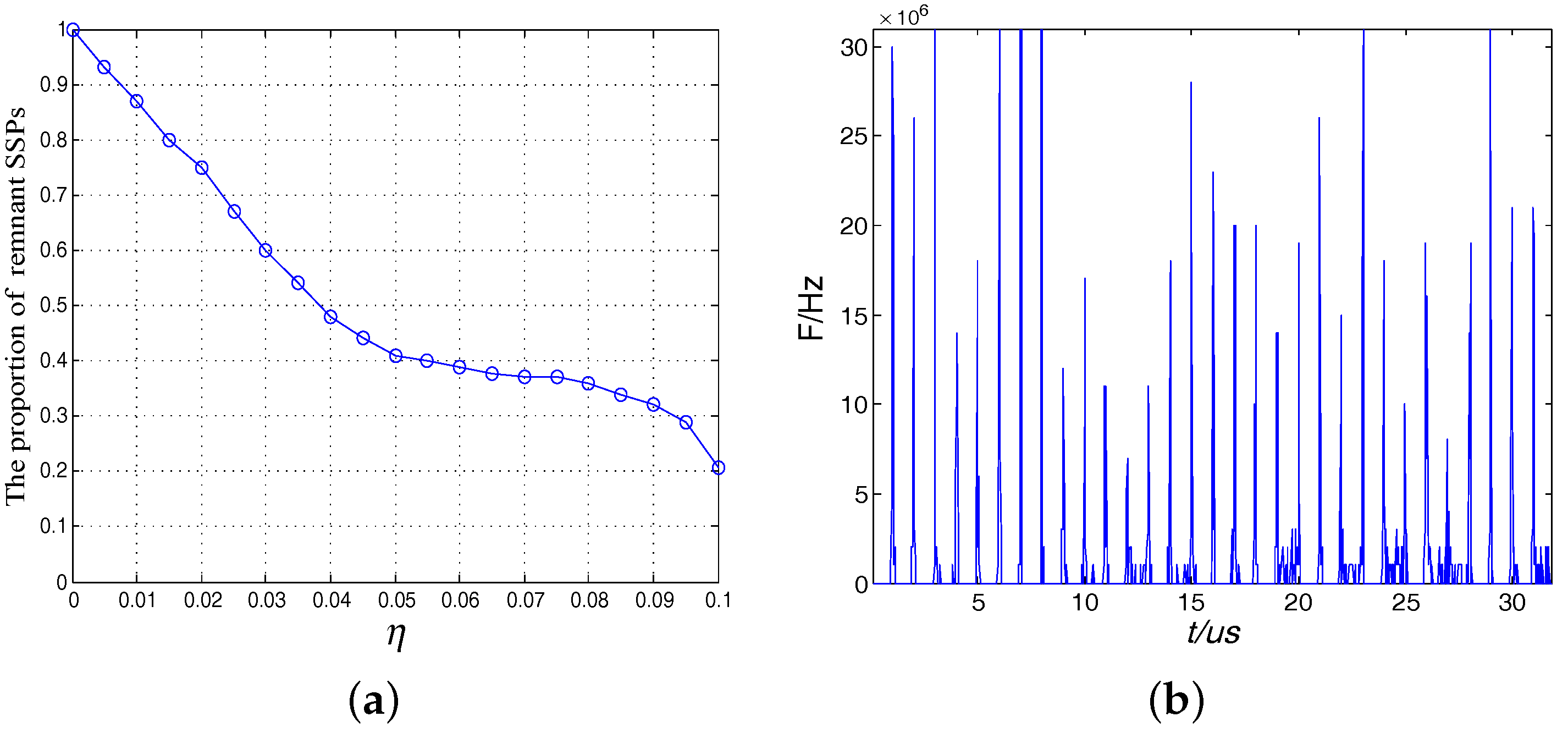
The TF scatter plots before and after the SSP detection of the observed signals are shown in Figure 1 and Figure 2, respectively. From Figure 1, it can be seen that, after noise pretreatment, the noise points are obviously reduced because the observed signal will show clear directions in the scatter plot, which depend on the column vectors of mixing matrix when the sources satisfy certain sparse conditions. Therefore, the scattered points away from these directions are considered to be noise points, which will seriously affect the accuracy of the algorithm in the mixing matrix estimation and subsequent source signal recovery. From Figure 2, we know that the directions and clustering of the observed signals become clearer after argument-based SSP detection. In general, based on the research of the former scholars [7], the value of threshold ranges from 0.01 to 0.1. In this paper, we give out the relationship curve between and the remnant SSPs. The proportion of remnant SSPs in all TF points is shown in Figure 3a, when the ratio tends to decrease in a gentle but steady manner, which means that most of the multiple-sources-points are removed. Thus, is chosen in this experiment.
Then, we utilize the hierarchical clustering technique for the estimation of the mixing matrix . The estimated after employing the noise pretreatment, SSP detection and clustering algorithm is
5.4. Experiment 2 and Analysis
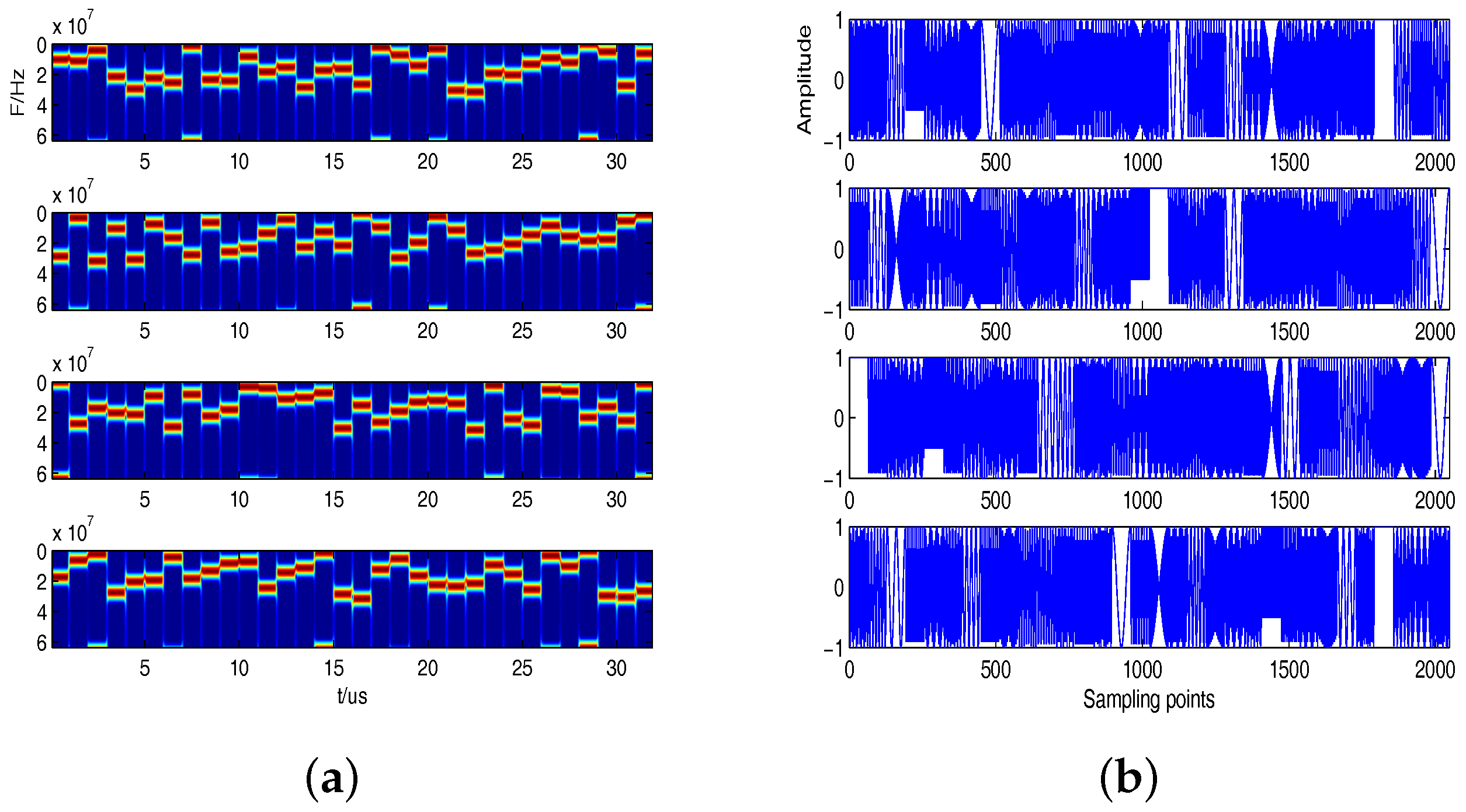
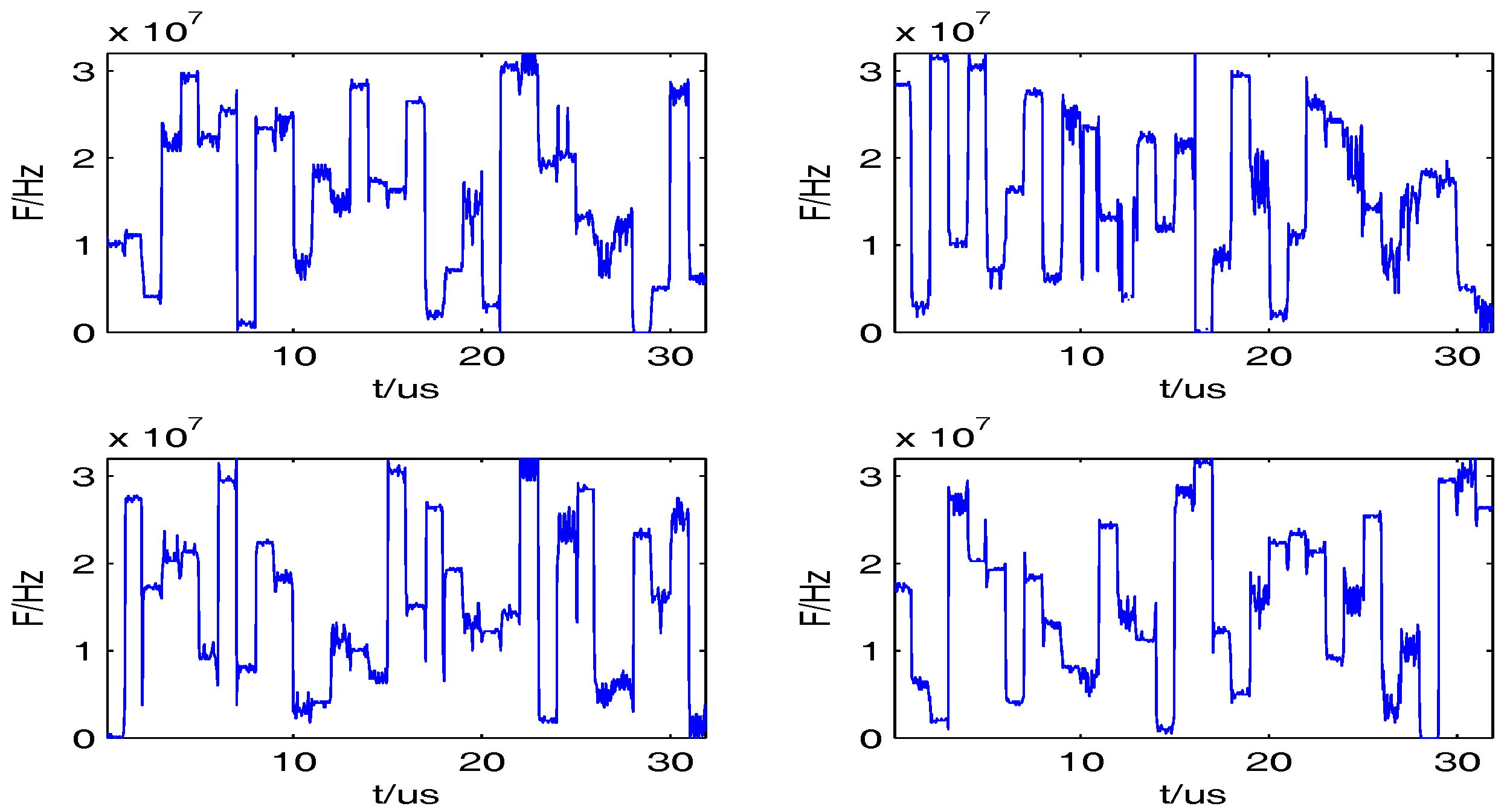
In this experiment, we use the sources and the estimated mixing matrix in Experiment 1, SNR = 20 dB. The TF and time domain diagrams of the four sources are shown in Figure 4a,b. From Figure 4b, we know that MIMO radar signals are continuous waves in the time domain, and the sparsity is weak, so that the traditional time domain sparse reconstruction algorithm cannot play its effectiveness. From Figure 4a, it can be seen that, although the ideal MIMO radar signals are orthogonal, but, in reality, it is difficult to meet, and there are certain overlaps of the frequency. Therefore, the DFCWs are insufficiently sparse in the time and frequency domains. The TF and time domains diagrams of the three observed signals are shown in Figure 5a,b. The TF-SL0 algorithm is used to reconstruct the TF diagram and time domain diagram, as shown in Figure 6a,b. From the Figure 6a, it can be seen that the effect of preliminary reconstruction in the TF domain is good except for the scale ambiguity of the BSS. In order to recover the time domain signals more accurately, TF ridge estimation algorithm is jointed to recover the TF information and the time domain waveforms of the sources by using the DFCW signal model. The TF ridges of the observed signals are shown in Figure 7. Figure 8 depicts the jumping-times of the coding sequences by smoothing and taking the frequency differences of TF ridges. From Equations (1) and (2), it can be seen that the duration of each pulse of each source signal is same, so, in order to get more precise jumping-times, we add the frequency differences corresponding to the jumping-times of four TF ridges and obtain Figure 3b. From Figure 3b, we know that when threshold , all the bogus jumping-times caused by noise can be removed. Then, the estimated coding period is obtained s by statistically averaging the differences of the jumping-times.The coding frequency is finally estimated as shown in Figure 9 according to steps (6) and (7) in Section 4.2.
5.5. Experiment 3 and Analysis
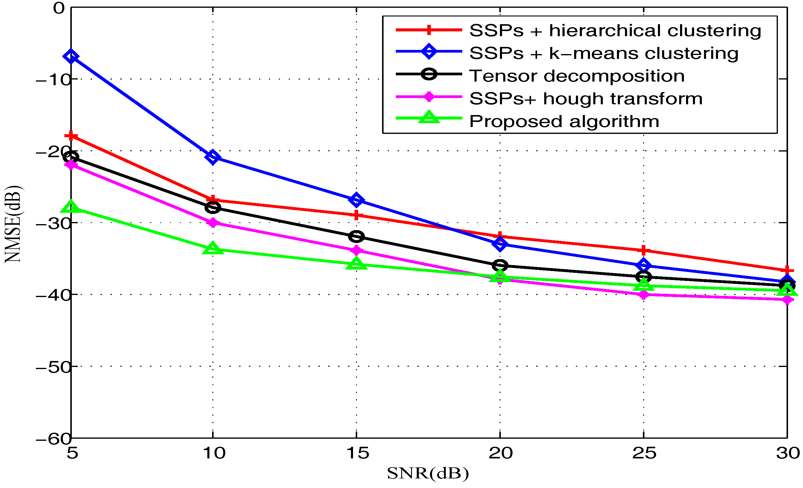
In order to evaluate the mixing matrix estimation precision of the proposed approach, the NMSE is utilized to compare with the proposed mixing matrix estimation algorithm in Section 3, the Reju algorithms in [7], the SSPs+ k-means clustering algorithms in [8], the SSPs+ Hough transform algorithms in [9] and the tensor decomposition algorithms in [23] by varying SNR from 5 dB to 30 dB. According to the setting ways of parameters and in Experiment 1, the parameters values are shown in Table 1. The results averaged over 50 Monte Carlo trials are shown in Figure 10. It can be seen from the figure that the proposed algorithm is robust to noise and estimates the mixing matrix with higher accuracy compared with the other algorithms. When the SNR is above 18 dB, the algorithm of Hough transform estimates the mixing matrix more accurately than other algorithms. However, the performance of the proposed algorithm is much more effective than the algorithms when the SNR is below 18 dB. The above results are mainly caused by two key reasons. First, because of the weak sparsity of four radar sources, the algorithm of K-means clustering cannot identify the SSPs efficiently. The hierarchical clustering algorithm can detect the SSPs, but the threshold of the hierarchical clustering cannot be determined easily in the noise case. Second, after the processing, most of the noise points are removed to eliminate the influence of the noise, while the noise will seriously affect the accuracy of the algorithm in the mixing matrix estimation based on tensor decomposition and Hough transform algorithms.
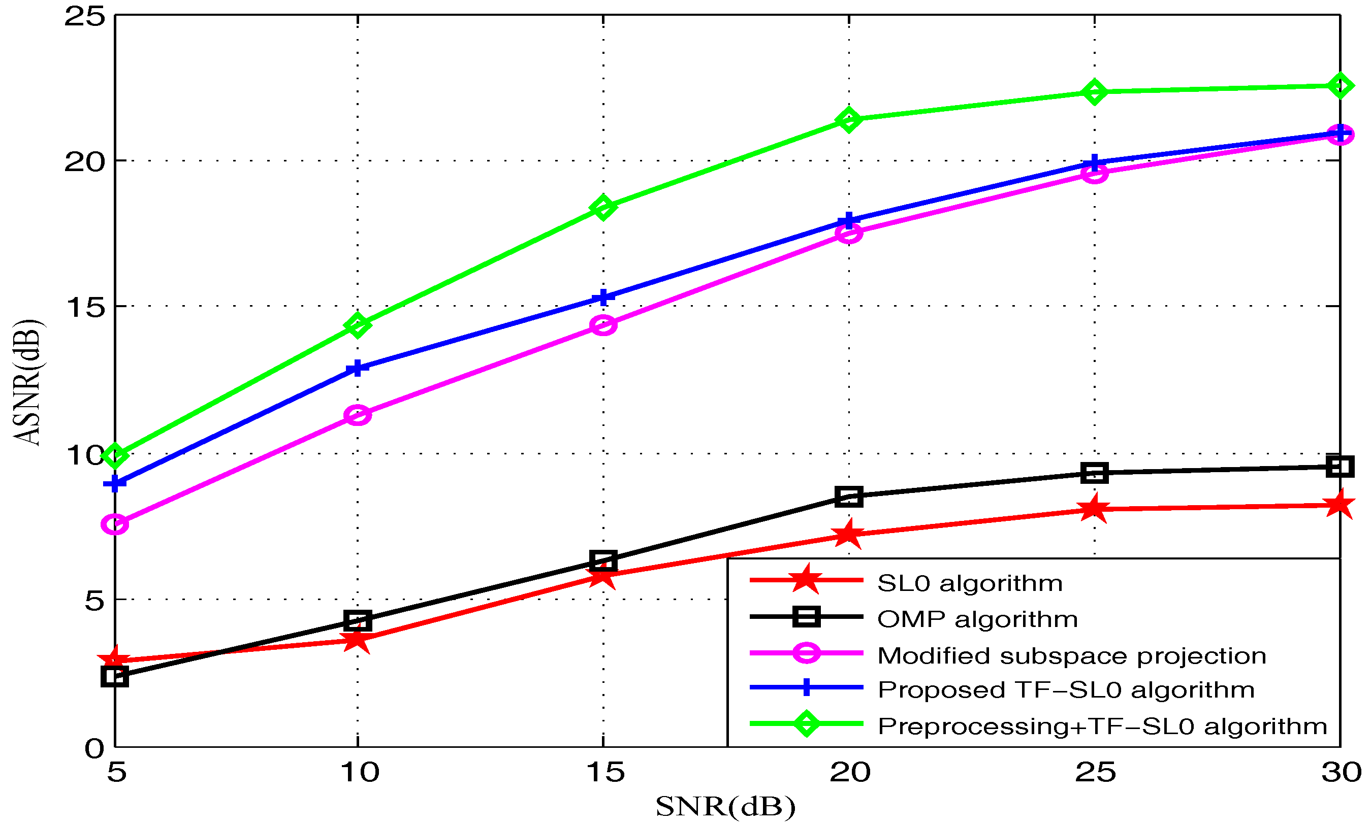
The mixing matrix has been estimated, similarly, using the ASNR to evaluate the recovery precision of the algorithm. The SL0 algorithm in [18], the OMP algorithm in [22], the subspace projection algorithm in [23], the proposed TF-SL0 algorithm and preprocessing +TF-SL0 algorithm are compared in the noisy case. The results averaged over 50 Monte Carlo trials are shown in Figure 11. From the figure, we know that the SL0 and OMP algorithms are basically invalid in the process of the signals’ recovery. The reason is that the radar signals are insufficiently sparse in both time and frequency domains, and consequently cannot meet the SL0 and OMP algorithms’ priori condition. The proposed TF-SL0 algorithm can make full use of the sparsity of the signals and the characteristics of the TF ridges, which obviously improves the ASNR of the recovered signals compared with subspace projection algorithm. Meanwhile, pretreatment +TF-SL0 algorithm reduces the effect of noise on the signals’ recovery, and improves the robustness and accuracy of the reconstruction, which verifies the validity of the proposed algorithm.
6. Conclusions
In order to address the separation problem of underdetermined MIMO radar signals when the sources are insufficiently sparse in both time and frequency domains, the noise preprocessing algorithm and SSP detection are employed to improve SNR and signal sparsity. Then, a modified TF-SL0 algorithm is proposed to complete the recovery of MIMO radar signals by the jointing SL0 algorithm with TF ridge estimation in the TF domain. Simulation results indicate that the proposed method can recover sources with higher accuracy compared with other algorithms in the experiments. In this paper, the determination of the coding period requires presetting parameters, so exploring more efficient TF ridge estimation algorithms will be the next research direction.
Acknowledgments
This work is supported by the National Natural Science Foundation of China (No. 61371172), the International S&T Cooperation Program of China (ISTCP) (No. 2015DFR10220), and the Fundamental Research Funds for the Central Universities (No. HEUCF1508).
Author Contributions
Qiang Guo and Guoqing Ruan conceived and designed the study. Guoqing Ruan and Qiang Guo performed the experiments. Guoqing Ruan wrote the paper. Qiang Guo, Guoqing Ruan and Yanping Liao reviewed and edited the manuscript. All authors read and approved the manuscript.
Conflicts of Interest
The authors declare that there is no conflict of interests regarding the publication of this paper.
References
- Zhang, H.; Wang, G.; Cai, P.; Wu, Z.; Ding, S. A fast blind source separation algorithm based on the temporal structure of signals. Neurocomputing 2014, 139, 261–271. [Google Scholar] [CrossRef]
- Tang, G.; Luo, G.G.; Zhang, W.H. Underdetermined Blind Source Separation with Variational Mode Decomposition for Compound Roller Bearing Fault Signals. Sensors 2016, 16, 897. [Google Scholar] [CrossRef] [PubMed]
- Li, Y.; Nie, W.; Ye, F.; Lin, Y. A Mixing Matrix Estimation Algorithm for Underdetermined Blind Source Separation. Circuits Syst. Signal Process. 2016, 35, 3367–3379. [Google Scholar] [CrossRef]
- Bofill, P.; Zibulevsky, M. Underdetermined blind source separation using sparse representations. Signal Process. 2001, 81, 2353–2362. [Google Scholar] [CrossRef]
- Jourjine, A.; Rickard, S. Blind separation of disjoint orthogonal signals: Demixing N sources from 2 mixtures. Acoust. Speech Signal Process. ICASSP 2000, 5, 2985–2988. [Google Scholar]
- Yilmaz, O.; Rickard, S. Blind separation of speech mixture via time-frequency masking. IEEE Trans. Signal Process. 2004, 52, 1830–1847. [Google Scholar] [CrossRef]
- Reju, V.G.; Koh, S.N.; Soon, I.Y. An algorithm for mixing matrix estimation in instantaneous blind source separation. Signal Process. 2009, 89, 1762–1773. [Google Scholar] [CrossRef]
- Kim, S.G.; Yoo, C.D. Underdetermined blind source separation based on subspace representation. IEEE Trans. Signal Process. 2009, 57, 2604–2614. [Google Scholar]
- Sun, J.; Li, Y.; Wen, J.; Yan, S. Novel mixing matrix estimation approach in underdetermined blind source separation. Neurocomputing 2016, 173, 623–632. [Google Scholar] [CrossRef]
- Mallat, S.G.; Zhang, Z. Matching pursuits with time-frequency dictionaries. IEEE Trans. Signal Process. 1993, 41, 3397–3415. [Google Scholar] [CrossRef]
- Chen, S.; Billings, S.A.; Luo, W. Orthogonal least squares methods and their application to non-linear system identification. Int. J. Control 1989, 50, 1873–1896. [Google Scholar] [CrossRef]
- Pati, Y.C.; Rezaiifar, R.; Krishnaprasad, P.S. Orthogonal matching pursuit: Recursive function approximation with applications to wavelet decomposition. In Proceedings of the Conference Record of the 27th Asilomar Conference on Signals Systems and Compute, Pacific Grove, CA, USA, 1–3 November 1993; Volume 1, pp. 40–44. [Google Scholar]
- Chen, S.S.; Donoho, D.L.; Saunders, M.A. Atomic decomposition by basis pursuit. SIAM Rev. 2001, 43, 129–159. [Google Scholar] [CrossRef]
- Zibulevsky, M.; Pearlmutter, B.A. Blind source separation by sparse decomposition in a signal dictionary. Neural Comput. 2001, 13, 863–882. [Google Scholar] [CrossRef] [PubMed]
- Donoho, D.L.; Elad, M. Maximal sparsity representation via l1 minimization. Proc. Natl. Acad. Sci. USA 2003, 100, 2197–2202. [Google Scholar] [CrossRef] [PubMed]
- Li, Y.Q.; Cichocki, A.; Amari, S.I. Analysis of sparse representation and blind source separation. Neural Comput. 2004, 16, 1193–1234. [Google Scholar] [CrossRef] [PubMed]
- Zayyani, H.; Babaie, Z.M.; Jutten, C. An iterative Bayesian algorithm for sparse component analysis in presence of noise. IEEE Trans. Signal Process. 2009, 57, 4378–4390. [Google Scholar] [CrossRef]
- Mohimani, H.; Babaie, Z.M.; Jutten, C. A fast approach for overcomplete sparse decomposition based on smoothed l0 norm. IEEE Trans. Signal Process. 2009, 57, 289–301. [Google Scholar] [CrossRef]
- Amishima, T.; Okamura, A.; Morita, S.; Kirimoto, T. Permutation method for ICA separated source signal blocks in time domain. IEEE Trans. Aerosp. Electron. Syst. 2010, 46, 899–904. [Google Scholar] [CrossRef]
- Feger, R.; Pfeffer, C.; Stelzer, A. A frequency-division MIMO FMCW radar system based on Delta–Sigma modulated transmitters. IEEE Trans. Microw. Theory Tech. 2014, 62, 3572–3581. [Google Scholar] [CrossRef]
- Ma, J.; Huang, G.; Zhou, D.; Fang, B.; Yu, H. Underdetermined blind sorting of radar signals based on sparse component analysis. In Proceedings of the IEEE International Conference on Communication Technology, Chengdu, China, 9–11 November 2012; pp. 1296–1300. [Google Scholar]
- Fang, B.; Huang, G.; Gao, J. Underdetermined blind source separation for LFM radar signal based on compressive sensing. In Proceedings of the 2013 25th Chinese Control and Decision Conference, Guiyang, China, 25–27 May 2013; pp. 1878–1882. [Google Scholar]
- Ai, X.F.; Luo, Y.; Zhao, G.Q. Underdetermined blind separation of radar signals based on tensor decomposition. Syst. Eng. Electron. 2016, 38, 2505–2509. [Google Scholar]
- Liu, B.; He, Z. Comments on discrete frequency-coding waveform design for netted radar systems. IEEE Signal Process. Lett. 2008, 15, 449–451. [Google Scholar] [CrossRef]
- Xu, R.; Wunsch, D. Survey of clustering algorithms. IEEE Trans. Neural Netw. 2005, 16, 645–678. [Google Scholar] [CrossRef] [PubMed]
- Rivet, B.; Vigneron, V.; Paraschiv-Ionescu, A.; Jutten, C. Wavelet de-noising for blind source separation in noisy mixtures. In Independent Component Analysis and Blind Signal Separation; Lecture Notes in Computer Science; Springer: Berlin, Germany, 2004; Volume 3195, pp. 263–270. [Google Scholar]
- Liu, B. Orthogonal discrete frequency-coding waveform set design with minimized autocorrelation sidelobes. IEEE Trans. Aerosp. Electron. Syst. 2009, 45, 1650–1657. [Google Scholar] [CrossRef]
Figure 1.
The scatter plots of the observed signals before single source point (SSP) detection. (a) without noise pretreatment; (b) after noise pretreatment.
Figure 1.
The scatter plots of the observed signals before single source point (SSP) detection. (a) without noise pretreatment; (b) after noise pretreatment.
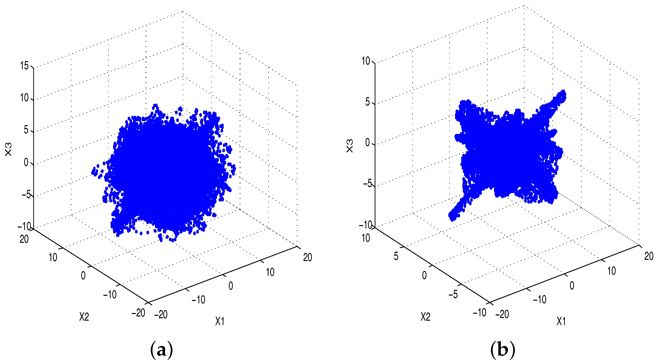
Figure 2.
The scatter plots of the observed signals after SSP detection. (a) without noise pretreatment; (b) after noise pretreatment.
Figure 2.
The scatter plots of the observed signals after SSP detection. (a) without noise pretreatment; (b) after noise pretreatment.
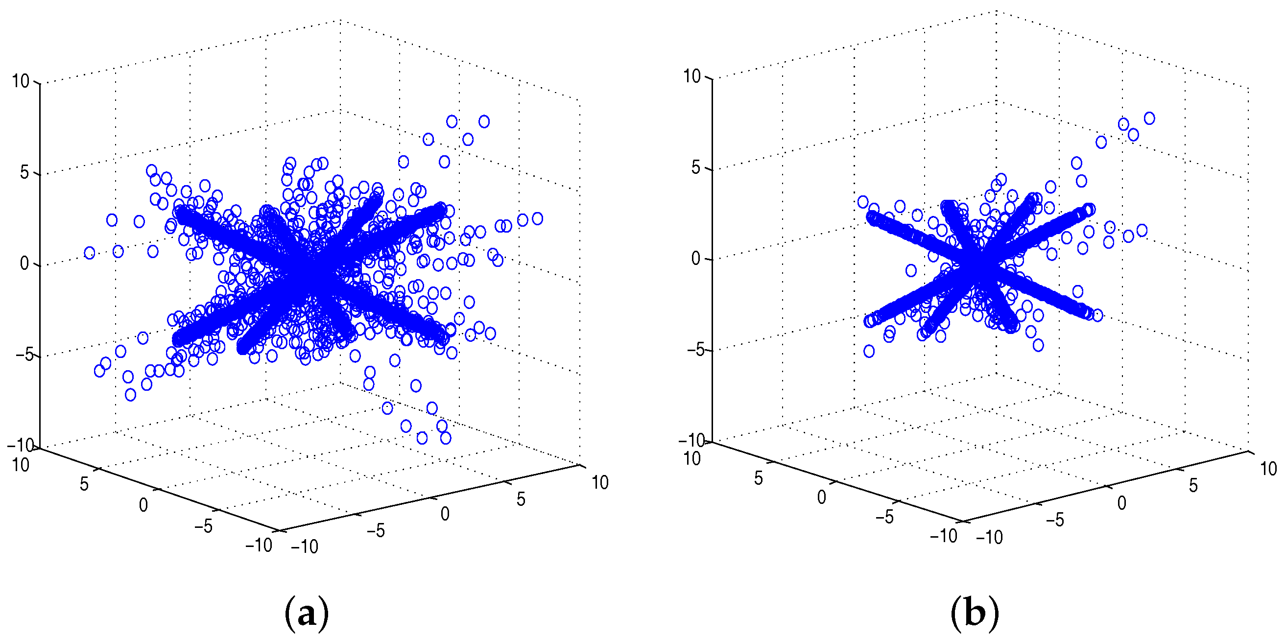
Figure 3.
Parameter setting. (a) the proportion of remnant SSPs in all time-frequency (TF) points; (b) the sum of the frequency differences corresponding to the jumping-times of four TF ridges.
Figure 3.
Parameter setting. (a) the proportion of remnant SSPs in all time-frequency (TF) points; (b) the sum of the frequency differences corresponding to the jumping-times of four TF ridges.

Figure 4.
The TF and time domains diagrams of the four sources. (a) in TF domain; (b) in time domain.
Figure 4.
The TF and time domains diagrams of the four sources. (a) in TF domain; (b) in time domain.

Figure 5.
The TF and time domains diagrams of the observed signals. (a) in TF domain; (b) in time domain.
Figure 5.
The TF and time domains diagrams of the observed signals. (a) in TF domain; (b) in time domain.
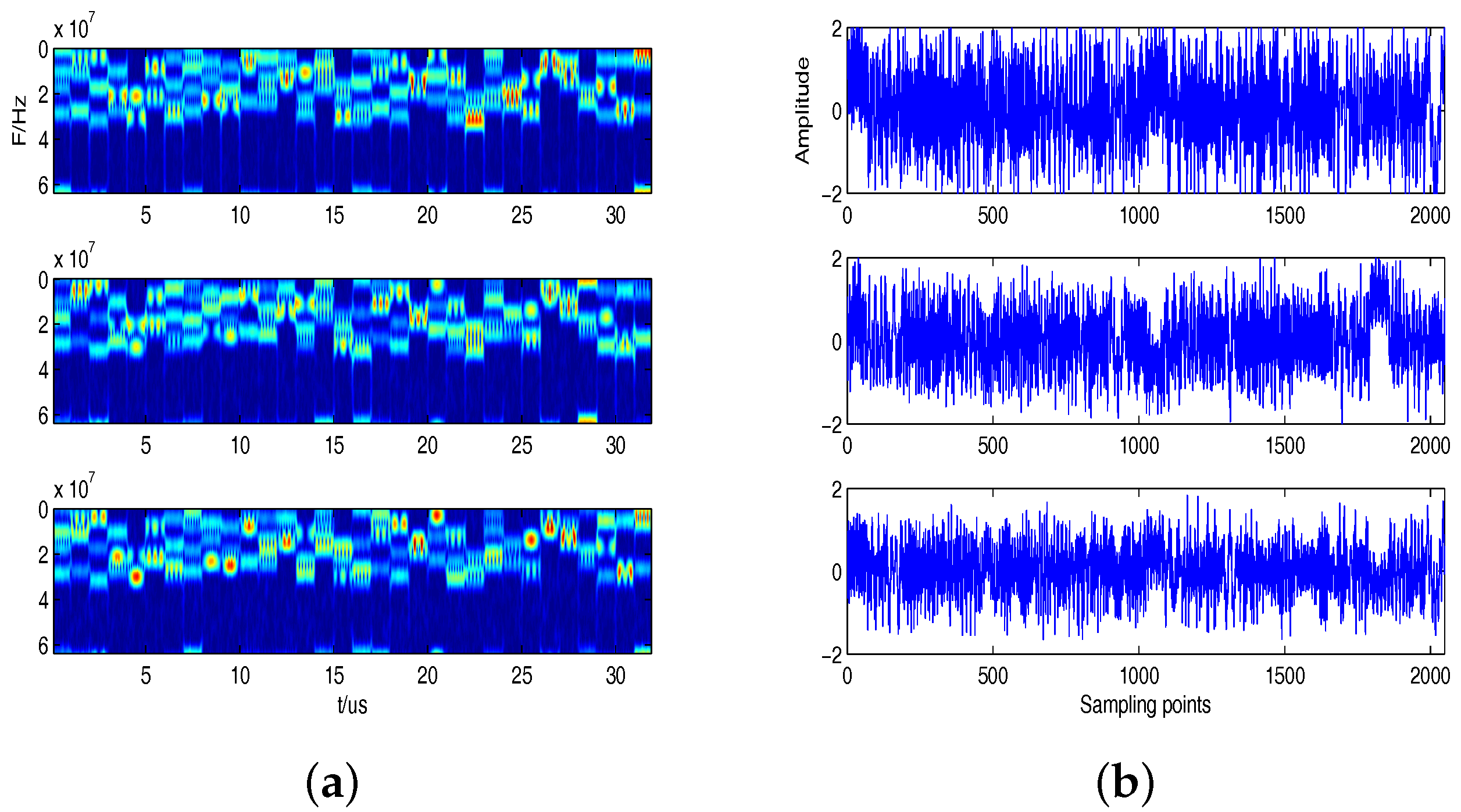
Figure 6.
The TF and time domains diagrams of the recovery signals. (a) in TF domain; (b) in time domain.
Figure 6.
The TF and time domains diagrams of the recovery signals. (a) in TF domain; (b) in time domain.
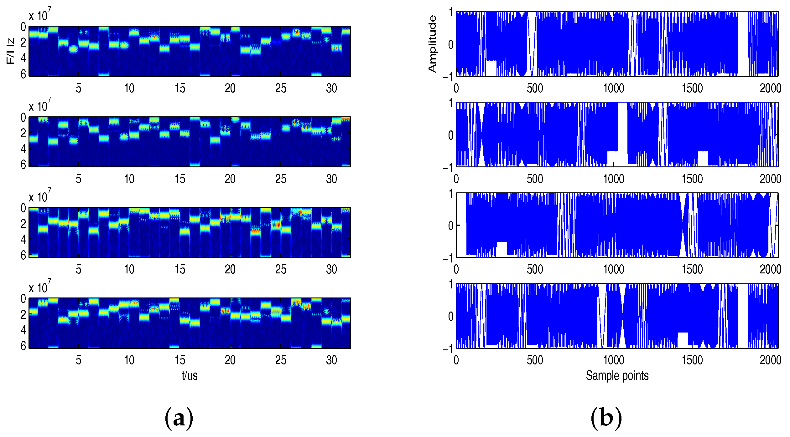
Figure 7.
The estimated TF ridges of the four recovery signals.

Figure 8.
The estimated jumping-times of the coding sequences of the four recovery signals.
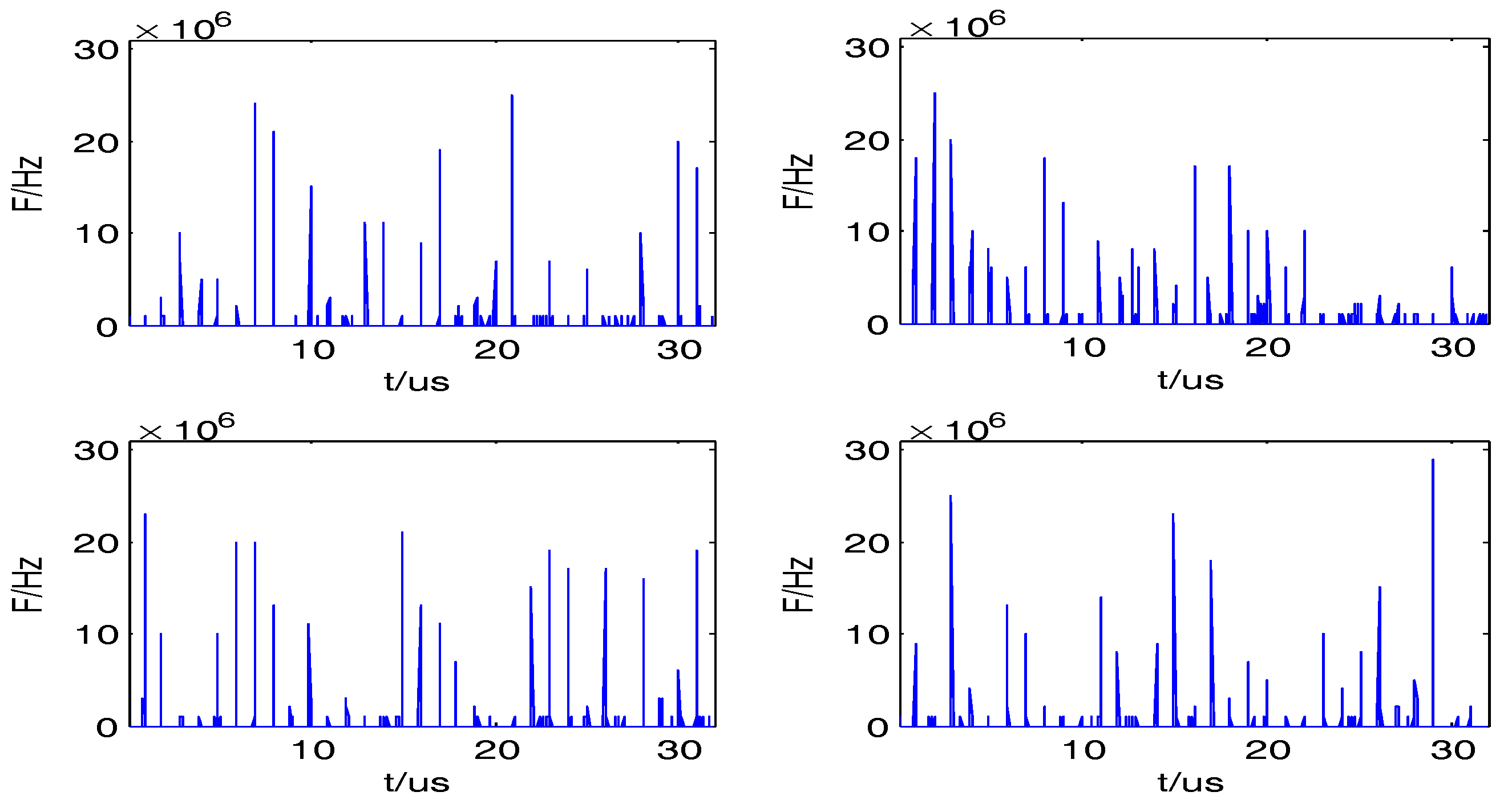
Figure 9.
The estimated coding frequency of the four recovery signals.
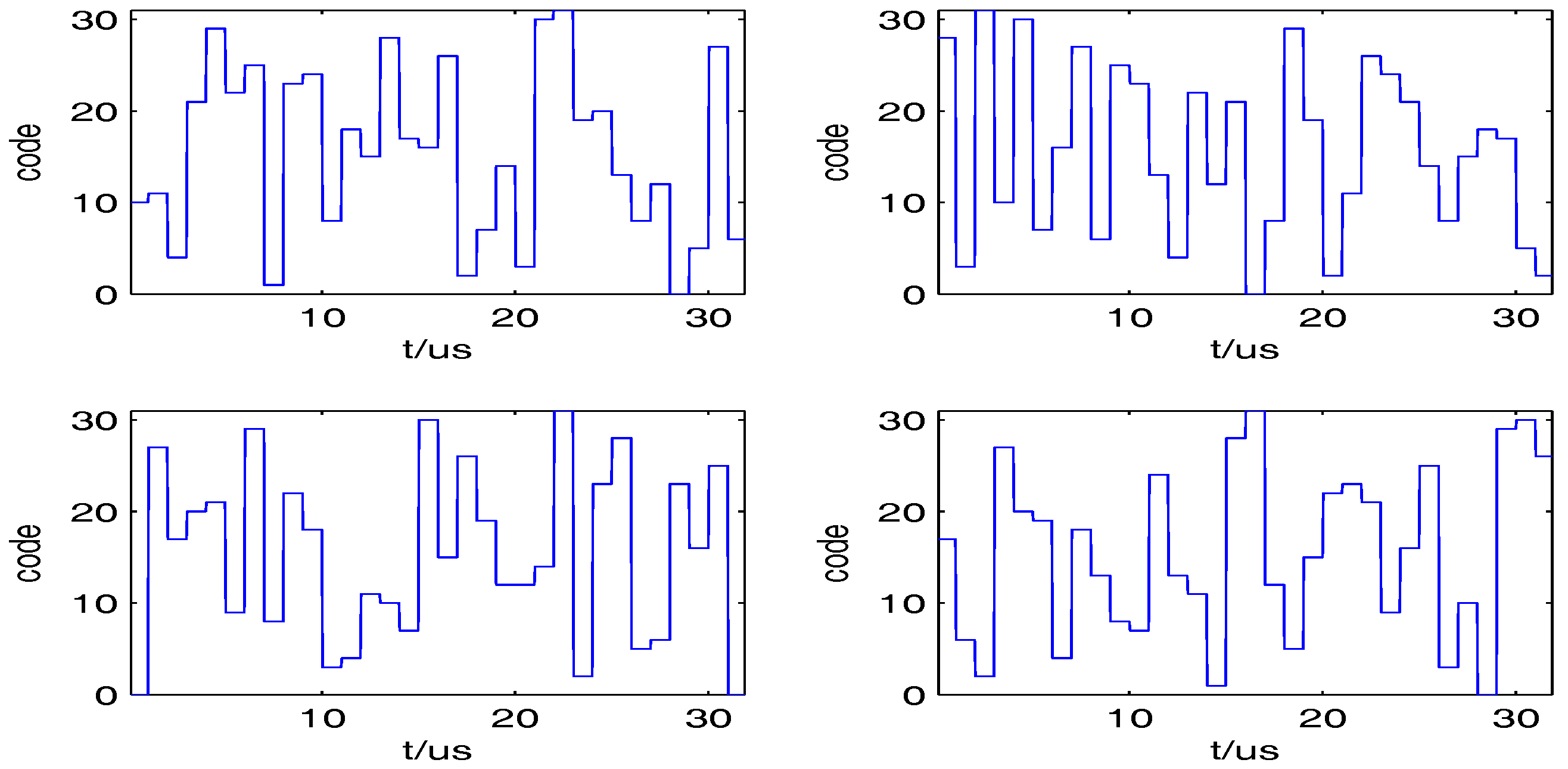
Figure 10.
Performances of the proposed and other algorithms to estimate mixing matrix in the noisy case. NMSE: Normalized mean square error.
Figure 10.
Performances of the proposed and other algorithms to estimate mixing matrix in the noisy case. NMSE: Normalized mean square error.

Figure 11.
Performances of the proposed and other algorithms to reconstruct signals in the noisy case. ASNR: Average recovered signal-to-noise ratio; SL0: Smoothed norm; OMP: Orthogonal matching pursuit; TF-SL0: Time-frequency smoothed norm.
Figure 11.
Performances of the proposed and other algorithms to reconstruct signals in the noisy case. ASNR: Average recovered signal-to-noise ratio; SL0: Smoothed norm; OMP: Orthogonal matching pursuit; TF-SL0: Time-frequency smoothed norm.

Table 1.
The parameter values by the setting method in Experiment 1 under different signal-to-noise ratios (SNRs).
Table 1.
The parameter values by the setting method in Experiment 1 under different signal-to-noise ratios (SNRs).
| SNR | 5 dB | 10 dB | 15 dB | 20 dB | 25 dB | 30 dB |
|---|---|---|---|---|---|---|
| 0.02 | 0.035 | 0.045 | 0.05 | 0.052 | 0.055 | |
| () | 6.5 | 6.2 | 5.8 | 5.0 | 5.0 | 5.0 |
© 2017 by the authors. Licensee MDPI, Basel, Switzerland. This article is an open access article distributed under the terms and conditions of the Creative Commons Attribution (CC BY) license (http://creativecommons.org/licenses/by/4.0/).
Share and Cite
MDPI and ACS Style
Guo, Q.; Ruan, G.; Liao, Y. A Time-Frequency Domain Underdetermined Blind Source Separation Algorithm for MIMO Radar Signals. Symmetry 2017, 9, 104. https://doi.org/10.3390/sym9070104
AMA Style
Guo Q, Ruan G, Liao Y. A Time-Frequency Domain Underdetermined Blind Source Separation Algorithm for MIMO Radar Signals. Symmetry. 2017; 9(7):104. https://doi.org/10.3390/sym9070104
Chicago/Turabian StyleGuo, Qiang, Guoqing Ruan, and Yanping Liao. 2017. "A Time-Frequency Domain Underdetermined Blind Source Separation Algorithm for MIMO Radar Signals" Symmetry 9, no. 7: 104. https://doi.org/10.3390/sym9070104
Note that from the first issue of 2016, this journal uses article numbers instead of page numbers. See further details here.