Cloud Generalized Power Ordered Weighted Average Operator and Its Application to Linguistic Group Decision-Making

Abstract

In this paper, we develop a new linguistic aggregation operator based on the cloud model for solving linguistic group decision-making problem. First, an improved generating cloud method is proposed so as to transform linguistic variables into clouds, which modifies the limitation of the classical generating cloud method. We then address some new cloud algorithms, such as cloud possibility degree and cloud support degree which can be respectively used to compare clouds and determine the weights. Combining the cloud support degree with power aggregation operator, we develop a new cloud aggregation operator dubbed the cloud generalized power ordered weighted average (CGPOWA) operator. We study the properties of the CGPOWA operator and investigate its family including a wide range of aggregation operators such as the CGPA operator, CPOWA operator, CPOWGA operator, CPWQA operator, CWAA and CWGA operator. Furthermore, a new approach for linguistic group decision-making is presented on the basis of the improved generating cloud method and CGPOWA operator. Finally, an illustrative example is provided to examine the effectiveness and validity of the proposed approach.

1. Introduction

As an important part of modern decision science, multiple criteria decision-making (MCDM) is the process of finding the best option from all of the feasible alternatives. It consists of a single decision maker (DM), multiple decision criteria and multiple decision alternatives [1]. However, the increasing complexity of the socioeconomic environment makes it less possible for a single DM to consider all relevant aspects of a problem as many decision-making processes take place in group settings. This makes the multiple criteria group decision-making (MCGDM) become more and more attractive in management [2,3,4,5,6]. Due to the complexities of objects and the vagueness of the human mind, it is more appropriate for the DMs to use linguistic descriptors than other descriptors to express their assessments in the actual process of MCGDM [7,8,9]. For example, when evaluating the “comfort” or “design” of a car, terms such as “good”, “medium”, and “bad” are frequently used, and when evaluating a car’s speed, terms such as “very fast”, “fast”, and “slow” can be used instead of numerical values. In such situations, the use of a linguistic approach is necessary. The objective of Linguistic multiple criteria group decision-making (LMCGDM) is to find the optimal solution(s) from a set of feasible alternatives by means of linguistic information provided by the DMs. To realize this objective, aggregating linguistic information is the key point and linguistic aggregation operators are commonly used.

Until now, many linguistic aggregation operators have been proposed and these operators can be classified into six types: (1) the first is based on linear ordering, such as the linguistic max and min operators [10,11,12], linguistic max-min weighted averaging operator [13], linguistic median operator [14], ordinal ordered weighted averaging operator [15], linguistic weighted conjunction operator [16]; (2) The second is built on the extension principle [17,18] and makes computations on fuzzy numbers that support the semantics of the linguistic labels, such as the linguistic OWA operator [19], and the linguistic weighted OWA operator [20], the inverse linguistic OWA operator degree [21], distance measure operator with linguistic information [22], induced linguistic continuous ordered weighted geometric operator [23], linguistic distances with continuous aggregation operator [24], linguistic probabilistic weighted average operator [25]; (3) The third is based upon 2-tuple representation, including the 2-tuple arithmetic mean operator [26], 2-tuple OWA operator [27], dependent 2-tuple ordered weighted geometric operator [28], 2-Tuple linguistic hybrid arithmetic aggregation operator [29]; (4) The fourth computes directly with words, such as the linguistic weighted averaging operator [30], extended ordered weighted geometric operator [31], linguistic weighted arithmetic averaging operator [32], linguistic ordered weighted geometric averaging operator [33], uncertain linguistic weighted averaging operator [34], induced uncertain linguistic OWA operator [35], uncertain linguistic geometric mean operator [36]; (5) The fifth is on the basis of the power ordered weighted average operator [37], including linguistic power ordered weighted average (LPOWA) operator [38], the linguistic generalized power average (LGPA) operator [39]; (6) and the last is a class of cloud aggregation operator which introduces the cloud model [40], in LMCGDM, such as the cloud weighted arithmetic averaging (CWAA) operator and cloud weight geometric averaging (CWGA) operator [41], trapezium cloud ordered weighted arithmetic averaging (TCOWA) operator [42]. A detail description of the operators LPOWA, CCWA, and CWGA will be presented in Section 2 of the paper.

The above mentioned operators of types (1)–(2) develop approximation processes to express the results in the initial expression domain, but they produce a consequent loss of information and then result in a lack of precision [26]. This shortcoming of operators of types (1)–(2) is just overcome by those operators of types (3)–(4) which allow a continuous representation of the linguistic information on their domains, and then can represent any counting of information obtained in an aggregation process without loss of information [26,27,28,29]. However, the operators of types (3)–(4) do not consider the information about the relationship between the values being combined [38]. The weakness of operators of types (3)–(4) can be corrected by operators of type (5) since they allow exact arguments to support each other in aggregation process and the weighting vectors depend on the input arguments and allow values to be aggregated to support and reinforce each other [37,38,39]. In this way, operators of type (5) consider the information about the relationship between the values being fused, but these operators of type (5) cannot describe the randomness of languages [41].

The limitation of operators of type (5) can be explained by the following fact. We know that natural languages generally include uncertainty in which randomness and fuzziness are the two most important aspects; here, the fuzziness mainly refers to uncertainty regarding the range of extension of concept, and the randomness implies that any concept is related to the external world in various ways [42]. The fuzziness and randomness are used to describe the uncertainty of natural languages. For instance, for a linguistic decision-making problem, DM A may think that 75% fulfillment of a task is “good”, but DM B may regard that less than 80% fulfillment of the same task cannot be considered as “good” with the same linguistic term scale. In this way, when considering the degree of certainty of an element belonging to a qualitative concept in a specific universe, it is more feasible to allow a stochastic disturbance of the membership degree encircling a determined central value than to allow a fixed number [41,42]. The cloud model, based on the fuzzy set theory and probability statistics [40,43,44], can describe the fuzziness with a normal membership function and the randomness by means of three numerical characteristics (expectation, entropy and Hyper entropy). Hence, the cloud aggregation operators of type (6) just overcome the limitation of operators of type (5). Nevertheless, the cloud aggregation operators of type (6) do not take into account the information about the relationship between the values being fused.

Based on the above analyses, we find that the limitations of linguistic power aggregation operators of type (5) and cloud aggregation operators of type (6) are mutually complementary. In other words, the linguistic power aggregation operators focus on the information about the relationship between the values being fused, while they ignore the randomness of qualitative concept; the cloud aggregation operators can capture the fuzziness and randomness of linguistic information, but they neglect the information about the relationship between values being fused.

Therefore, this paper aims to propose a new cloud generalized power ordered weighted average (CGPOWA) operator so as to overcome the limitations of existing linguistic power aggregation operators of (5) and cloud aggregation operators of (6). The novelty of this paper is as follows.

(i)

We present an improved generating cloud method to transform linguistic variables into clouds. The key to linguistic decision-making based on cloud models is the transformation between linguistic variables and clouds, for which Wang and Feng [45] proposed a method of generating five clouds on the basis of the golden ratio, but this method has three weaknesses: (a) it is limited to a linguistic term set of 5 labels; (b) the expectation of clouds sometimes exceeds the range of the universe; and (c) it cannot effectively distinguish the linguistic evaluation scale over the symmetrical interval. Regarding these limitations, we present an improved method by applying the cloud construction principle. This method can transform linguistic term set of any odd labels rather than only five labels, and can guarantee that all the expectations of clouds fall into the range of the universe. Meanwhile, it can effectively distinguish the linguistic evaluation scale over the symmetrical interval. In this way, this method modifies the weaknesses of the classical generating cloud method.

(ii)

We address some new cloud algorithms such as cloud possibility degree and cloud support degree. Based on “3En rules” of cloud model, a cloud distance is defined. We further put forward to a cloud possibility degree according to this cloud distance, which can be used to compare the clouds, and define a cloud support degree which is a similarity index. That is, the greater the similarity is, the closer the two clouds are, and consequently the more they support each other. The support degree can be used to determine the weights of aggregation operator.

(iii)

We develop a new CGPOWA operator. By using the cloud support degree we defined and the power aggregation operator [39], we develop the CGPOWA operator, which overcomes the limitations of existing linguistic power aggregation operators and cloud aggregation operators and simultaneously maintains the advantages of the two types operators. By studying its properties, we find that the CGPOWA operator is idempotent, commutative and bounded. In addition, we investigate the family of the CGPOWA operator which contains a wide range of aggregation operators such as the CGPA operator, CPOWA operator, CPOWGA operator, CPWQA operator, CWAA and CWGA operators, the maximum and minimum operators.

(iv)

A new approach for LMCGDM is developed by applying the improved generating cloud method and CGPOWA operator. The main advantage of this approach is that it gives a completely objective view of the decision problem because the CGPOWA operator and the weighting method depend on the arguments completely. Comparing our method with three traditional LMCGDM approaches (linguistic symbolic model, linguistic membership function model, 2-tuple linguistic model) and the cloud aggregating method [41,42], we find that:

(a)

Compared with the three traditional LMCGDM approaches, our method takes a multi-granular linguistic assessment scale of great psychological sense, while the three traditional LMCGDM approaches only use a uniform granular linguistic assessment scale. In other words, when the alternatives are assessed, these three traditional approaches only regard the average level as the unique criterion, which leads to the evaluations rough and one-sided. Our method, however, considers not only the average level but also the fluctuation and stability of qualitative concepts via the cloud model;

(b)

Compared with cloud aggregating method [41,42], our method provides a completely objective weighting model by using the cloud support degree, while the weights in Wang et al. [41,42] are subjectively given by the DMs which may result in different ranking results if the DMs provide different weight vectors. In addition, the CGPOWA operator considers the relationships between the arguments provided by the DMs, while the cloud aggregating operators in Wang et al. [41,42] do not;

(c)

Our method presents a simple measure to compare different clouds by the cloud possibility degree (Equation (11)) and the ranking vector (Equation (13)), which requires no knowledge about the distribution of cloud drops, this is different from the score function [41] which needs to know the distribution of cloud drops. This is also an attractive feature because in most case the distribution of cloud drops is unknown and it is rigid to acquire cloud drops.

This approach is also applicable to different linguistic decision-making problems such as strategic decision-making, human resource management, product management and financial management.

The rest of the paper is organized as follows. Section 2 reviews the LPOWA, CWAA and CWGA operators and the cloud model. Section 3 presents an improved method of transforming linguistic variables into clouds, and provides some new cloud algorithms. Section 4 develops the CGPOWA operator and studies its properties. Section 5 develops an approach for LMCGDM. Section 6 presents an illustrative example and the conclusions are drawn in Section 7.

2. Preliminaries

In this section, we briefly review the LPOWA operator, the definitions and operational rules of the clouds, CWAA operator and CWGA operator.

2.1. The LPOWA Operator

The linguistic approach is an approximate technique that represents qualitative aspects as linguistic values using linguistic variables. Let $S=\left\{s_i|i=-t,\dots ,t\right\}$ be a finite and completely ordered discrete term set, which stands for a possible value for a linguistic variable. For instance, a set of nine terms $S$ could be [8,23]:

$$\begin{array}{c}S=\{s_{-4}=\mathrm{extremely}\mathrm{poor},s_{-3}=\mathrm{very}\mathrm{poor},s_{-2}=\mathrm{poor},s_{-1}=\mathrm{medium}\mathrm{poor},s_0=\mathrm{fair},\\ s_1=\mathrm{medium}\mathrm{good},s_2=\mathrm{good},s_3=\mathrm{very}\mathrm{good},s_4=\mathrm{extremely}\mathrm{good}\}\end{array}$$

In many real problems, the input linguistic arguments may not match any of the original linguistic labels, or may be located between two of them. For such cases, Xu [36] presents some operational laws. Let $s_1=[s_{{\alpha }_1},s_{{\beta }_1}]$ and $s_2=[s_{{\alpha }_2},s_{{\beta }_2}]$, the operational rules are as follows:

(i)

$s_1\otimes s_2=[s_{{\alpha }_1},s_{{\beta }_1}]\otimes [s_{{\alpha }_2},s_{{\beta }_2}]=[s_{{\alpha }_1}\otimes s_{{\alpha }_2},s_{{\beta }_1}\otimes s_{{\beta }_2}]=[s_{{\alpha }_1{\alpha }_2},s_{{\beta }_1{\beta }_2}]$;

(ii)

$s^{\lambda }={[s_{\alpha },s_{\beta }]}^{\lambda }=[s_{{\alpha }^{\lambda }},s_{{\beta }^{\lambda }}]$, where $\lambda \in [0,1]$;

(iii)

$s_1\otimes s_2=s_2\otimes s_1$;

(iv)

${(s_1\otimes s_2)}^{\lambda }={s_1}^{\lambda }\otimes {s_2}^{\lambda }$, where $\lambda \in [0,1]$.

Yager [37] introduced a nonlinear ordered weighted-average aggregation tool, called the power ordered weighted average (POWA) operator, which can be defined as follows:

$$POWA\left(a_1,a_2,\cdots ,a_n\right)={\displaystyle \sum _{j=1}^n{w}_j{\beta }_j^{\lambda }},$$

(1)

where $w_j=g\left(\frac{R_j}{TV}\right)-g\left(\frac{R_{j-1}}{TV}\right),R_j={\displaystyle \sum _{i=1}^j{\beta }_i},TV={\displaystyle \sum _{i=1}^n{\beta }_i},V_{{\beta }_i}=1+T({\beta }_i),T({\beta }_i)={\displaystyle \sum _{\begin{array}{l}j=1\\ j\ne i\end{array}}^{n}Sup({\beta }_i,{\beta }_j)}.$

Here $Sup({\beta }_i,{\beta }_j)$ is the support for ${\beta }_i$ from ${\beta }_j$ such that $Sup({\beta }_i,{\beta }_j)\in [0,1]$, $Sup({\beta }_i,{\beta }_j)=Sup({\beta }_j,{\beta }_i)$ and $Sup({\beta }_i,{\beta }_j)\ge Sup(x,y)$ for $\left|{\beta }_i-{\beta }_j\right|<\left|x-y\right|$; and ${\beta }_i$ is the ith largest of the arguments, and the basic unit-interval monotonic (BUM) function $g(\cdot )$ satisfies $g\left(0\right)=0$, $g\left(1\right)=1$, $g\left(x\right)\ge g\left(y\right)$, if $x>y$.

Based on the POWA operator, Xu, Merigó and Wang [38] provided a linguistic power ordered weighted average (LPOWA) operator, which is defined as follows.

Definition 1 (Xu, Merigó and Wang, [38]).

Let $s_{{\alpha }_j}(j=1,2,\dots ,n)$ be a collection of linguistic variables, a linguistic power ordered weighted averaging (LPOWA) operator is a mapping LPOWA: ${\overline{S}}^n\to \overline{S}$, if

$$LPOWA\left(s_{{\alpha }_1},s_{{\alpha }_2},\dots ,s_{{\alpha }_n}\right)=\underset{j=1}{\overset{n}{\oplus }}{u}_j{s}_{{\alpha }_{\sigma (j)}}$$

(2)

where $\left(\sigma (1),\sigma (2),\dots ,\sigma (n)\right)$ is a permutation of $\left(1,2,\dots ,n\right)$ such that $s_{{\alpha }_{\sigma (j-1)}}\ge s_{{\alpha }_{\sigma (j)}}$ for all j, and

$$u_j=g\left(\frac{B_j}{TV}\right)-g\left(\frac{B_{j-1}}{TV}\right),B_j={\displaystyle \sum _{i=1}^j{V}_{\sigma (i)}},TV={\displaystyle \sum _{j=1}^n{V}_{\sigma (j)}},V_{\sigma (j)}=1+T(s_{{\alpha }_{\sigma (j)}}),$$

where $g:\left[0,1\right]\to \left[0,1\right]$ is a basic unit-interval monotonic (BUM) function satisfying $g\left(0\right)=0$, $g\left(1\right)=1$, $g\left(x\right)\ge g\left(y\right)$ if $x>y$. $T(s_{{\alpha }_{\sigma (j)}})$ denotes the support of the jth largest argument by all the other arguments.

Remark 1.

The LPOWA operator considers the linguistic information about the relationship between the values being combined since it allows exact arguments to support each other in aggregation process and the weighting vectors depend on the input arguments and allow arguments being aggregated to support each other. However, this type operator can not characterize the randomness of languages. Here the randomness implies that any language is related to the external world in various ways [44]. In fact, natural languages usually involve in randomness and fuzziness (refer to uncertainty regarding the range of extension of languages). For example, DM A thinks 75% fulfillment of a task is “good”, but DM B thinks that less than 80% fulfillment of the same task cannot be considered “good” with the same linguistic term scale. When considering the degree of certainty of an element belonging to a qualitative concept in a specific universe, it is more feasible to allow a stochastic disturbance of the membership degree encircling a determined central value than to allow a fixed number.

2.2. Cloud Model

The cloud model, based on the fuzzy set theory and probability statistics [40], can describe the fuzziness with membership function and the randomness via probability distribution.

Definition 2 (Li, Meng and Shi, [40]).

Let $U$ be a quantitative domain expressed by precise values, and C a qualitative concept on the domain. If the quantitative value x $(x\in U)$ is a random instantiation to C, whose membership $\mu \left(x\right)\in \left[0,1\right]$ for C is a random number with stable tendency:

$$\mu :U\to \left[0,1\right],\forall x\in U,x\mapsto \mu \left(x\right).$$

(3)

Then, the distribution of x on the domain is named as a cloud and each x is named as a droplet.

The normal cloud model is applicable and universal for it is based on normal distribution and on the Gauss membership function [43].

Definition 3 (Li and Du, [43]).

Suppose that $U$ is the universe of discourse and T is a qualitative concept in $U$. If $x\left(x\in U\right)$ is a random instantiation of concept T satisfying $x\sim N(Ex,E{n^{\prime }}^2)$ and $E{n}^{\prime }\sim N\left(En,H{e}^2\right)$ and the certainty degree of x belonging to T satisfies $\mu =\exp \left(-\frac{{\left(x-Ex\right)}^2}{2{\left(E{n}^{\prime }\right)}^2}\right)$, then the distribution of x in the universe $U$ is called a normal cloud.

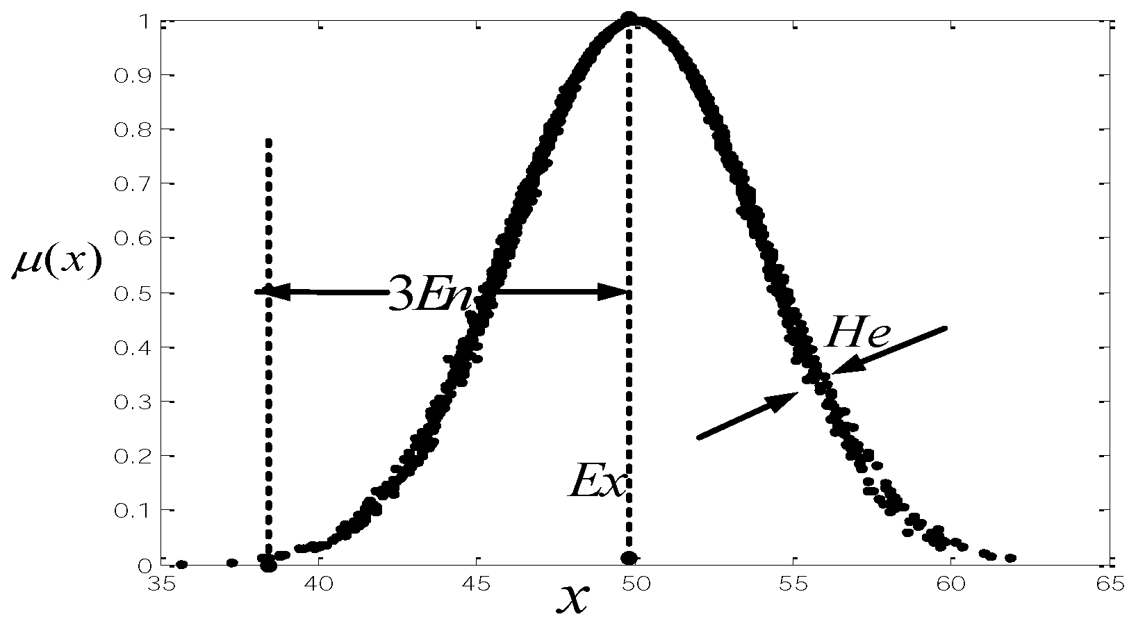
The cloud model can effectively integrate the randomness and fuzziness of concepts and describe the overall quantitative property of a concept via Expectation Ex, Entropy En, and Hyper entropy He. If A is a cloud with three numerical characteristics Ex, En, and He, then cloud A can be described as $A\left(Ex,En,He\right)$. Li, Liu and Gan [44] provided operation rules of clouds as follows. Assume that there are two clouds $A\left(E{x}_1,E{n}_1,H{e}_1\right)$ and $B\left(E{x}_2,E{n}_2,H{e}_2\right)$, operations between cloud A and cloud B are given by:

(i) 

$A+B=\left(E{x}_1+E{x}_2,\sqrt{E{n}_1^2+E{n}_2^2},\sqrt{H{e}_1^2+H{e}_2^2}\right)$;

(ii) 

$A-B=\left(E{x}_1-E{x}_2,\sqrt{E{n}_1^2+E{n}_2^2},\sqrt{H{e}_1^2+H{e}_2^2}\right)$;

(iii) 

$A\times B=\left(E{x}_1\times E{x}_2,\sqrt{{\left(E{n}_{1}E{x}_2\right)}^2+{\left(E{n}_{2}E{x}_1\right)}^2},\sqrt{{\left(H{e}_{1}E{x}_2\right)}^2+{\left(H{e}_{2}E{x}_1\right)}^2}\right)$;

(iv) 

$\lambda A=\left(\lambda E{x}_1,\sqrt{\lambda }E{n}_1,\sqrt{\lambda }H{e}_1\right)$;

(v) 

$A^{\lambda }=\left(E{x_1}^{\lambda },\sqrt{\lambda }E{x}_1^{\lambda -1}E{n}_1,\sqrt{\lambda }E{x}_1^{\lambda -1}H{e}_1\right)$.

Figure 1 shows that fuzziness is about the extension range of x, such as [37, 62]. Randomness is about the various cognitions for the DMs. In linguistic decision-making, there are occasions for which different individuals attribute different meanings to a linguistic expression. The same individual may even interpret the same linguistic expression differently in different situations. For instance, DM A may believe the membership degree of 45 belonging to the “number near 40” is 0.8, whereas DM B may regard it to be 0.85. Non-uniform cognition exists among the DMs. The process of aggregation of linguistic information will be distorted owing to the lack of uniformity. The cloud model allows the certainty degree of x to follow a probability distribution, which allows the distortion held by the DMs in the aggregation process to be neutralized to a great extent [41].

2.3. The CWAA Operator and CWGA Operator

Wang, Peng and Zhang [41] introduced the cloud model in LMCGDM and presented the cloud weighted arithmetic averaging (CWAA) operator and cloud weight geometric averaging (CWGA) operator.

Definition 4 (Wang, Peng and Zhang, [41]).

Let $\Omega$ be the set of all clouds and $Y_i(E{x}_i,E{n}_i,H{e}_i)$ $(i=1,2,\dots ,n)$ be a subset of $\Omega$. A mapping CWAA: ${\Omega }^n\to \Omega$ is defined as the cloud-weighted arithmetic averaging (CWAA) operator so that the following is true:

$$CWA{A}_{\omega }\left(Y_1,Y_2,\dots ,Y_n\right)={\displaystyle \sum _{i=1}^n{w}_i}{Y}_i,$$

(4)

Here $W=(w_1,w_2,\dots ,w_n)$ is the associated weight vector of $Y_i(E{x}_i,E{n}_i,H{e}_i)(i=1,2,\dots ,n)$, $w_i\in [0,1]$ $(i=1,2,\dots ,n)$ and ${\displaystyle \sum _{i=1}^n{w}_i}=1$.

Definition 5 (Wang, Peng and Zhang, [41]).

Let $\Omega$ be the set of all clouds and $Y_i(E{x}_i,E{n}_i,H{e}_i)$ $(i=1,2,\dots ,n)$ be a subset of $\Omega$. A mapping CWGA: ${\Omega }^n\to \Omega$ is defined as the CWGA operator, and the following is true:

$$CWG{A}_w\left(Y_1,Y_2,\dots ,Y_n\right)={\displaystyle \prod _{i=1}^n{Y}_i^{w_i}}$$

(5)

Remark 2.

The CWAA and CWGA operators characterize the fuzziness and randomness of languages with cloud model, while they do not take into account the information about the relationship between the values being fused.

3. An Improved Generating Cloud Method and Cloud Algorithms

This section provides an improved method to transform linguistic values into clouds, and define some new cloud algorithms, such as cloud possibility degree and cloud support degree.

3.1. An Improved Generating Cloud Method

For an LMCGDM problem, natural languages generally include vague and imprecise information which is too complex and ill-defined to describe by using conventional quantitative expressions, and thus there is a barrier for transforming linguistic information into quantitative values. The cloud model describes linguistic concepts via three numerical characteristics which realize the objective and interchangeable transformation between qualitative concepts and quantitative values. Hence, it is necessary to transform linguistic variables into clouds. The key of this transformation is to select a transformation method. As for this, Wang and Feng [45] proposed a classical method for generating five clouds on the basis of the golden ratio, which is equal of $\frac{1}{2}\left(1+\sqrt{5}\right)$.

Let n be the linguistic evaluation scale and $U=[X_{\min },X_{\max }]$ be an effective universe given by the DMs. Assume that the intermediate cloud is expressed by $Y_0(E{x}_0,E{n}_0,H{e}_0)$. The adjacent clouds around $Y_0(E{x}_0,E{n}_0,H{e}_0)$ are respectively expressed by:

$$\begin{gathered} Y_{-1}(E{x}_{-1},E{n}_{-1},H{e}_{-1}),Y_1(E{x}_1,E{n}_1,H{e}_1), \\ {Y}_{-2}(E{x}_{-2},E{n}_{-2},H{e}_{-2}),Y_2(E{x}_2,E{n}_2,H{e}_2), \\ \dots \dots , \\ {Y}_{-(n-1)/2}(E{x}_{-(n-1)/2},E{n}_{-(n-1)/2},H{e}_{-(n-1)/2}),Y_{(n-1)/2}(E{x}_{(n-1)/2},E{n}_{(n-1)/2},H{e}_{(n-1)/2}). \end{gathered}$$

The numerical characteristics of five clouds are shown as follows (Wang and Feng, [45]):

$$\begin{gathered} E{x}_0=\left(X_{\min }+X_{\max }\right)/2,E{n}_{-1}=E{n}_1=0.382\cdot \left(X_{\max }-X_{\min }\right)/6,E{n}_0=0.618E{n}_1, \\ E{n}_{-2}=E{n}_2=E{n}_1/0.618,E{x}_{-1}=E{x}_0-0.382\cdot \left(X_{\min }+X_{\max }\right)/2,E{x}_{-2}=X_{\min },E{x}_2=X_{\max }, \\ H{e}_{-1}=H{e}_1=H{e}_0/0.618,E{x}_1=E{x}_0+0.382\cdot \left(X_{\min }+X_{\max }\right)/2,H{e}_{-2}=H{e}_2=H{e}_1/0.618, \end{gathered}$$

Here $H{e}_0$ is given beforehand.

However, we find that there are three weaknesses in the method of Wang and Feng [45].

• First, the expectation of clouds may exceed the range of the universe $U$. For example, if $U=[10,20]$, then $E{x}_{-1}=E{x}_0-0.382\frac{X_{\min }+X_{\max }}{2}=9.27<10$, and $E{x}_1=E{x}_0+0.382\frac{X_{\min }+X_{\max }}{2}=20.73>20$.
• Second, the method of Wang and Feng [45] can not be widely used for it is only limited to five labels of the linguistic evaluation scale.
• And third, the method cannot effectively distinguish the linguistic evaluation scale over the symmetrical interval. For instance, if $U=[-a,a],a>0$, then the expectation values $E{x}_{-1}=E{x}_1=$ $E{x}_0=0$, which results in the linguistic evaluation scale undistinguished.

To overcome the above weaknesses, we present an improved method to transform linguistic variables into clouds by means of the cloud construction principle, which is shown as follows.

Procedure for transforming linguistic variables into clouds:

Step 1. Calculate $Ex$

$$\begin{gathered} E{x}_0=\left(X_{\min }+X_{\max }\right)/2,E{x}_i=E{x}_0+0.382i\left(\frac{X_{\max }-X_{\min }}{2}\right)/\frac{\left(n-3\right)}{2},E{x}_{(n-1)/2}=X_{\max } \\ E{x}_{-(n-1)/2}=X_{\min },E{x}_{-i}=E{x}_0-0.382i\left(\frac{X_{\max }-X_{\min }}{2}\right)/\frac{\left(n-3\right)}{2},(1\le i\le \frac{n-3}{2}). \end{gathered}$$

Step 2. Compute $En$

$$E{n}_{-1}=E{n}_1=0.382\times \left(X_{\max }-X_{\min }\right)/6,E{n}_0=0.618E{n}_{+1},E{n}_{-i}=E{n}_i=\frac{E{n}_{i-1}}{0.618},(2\le i\le \frac{n-1}{2}).$$

Step 3. Calculate $He$

$H{e}_{-i}=H{e}_{+i}=H{e}_{i-1}/0.618,1\le i\le \left(n-1\right)/2$, here $H{e}_0$ is given beforehand.

The following Theorem proves that our method can overcome the weaknesses of method given by Wang and Feng [45].

Theorem 1.

Let n be the linguistic evaluation scale and $U=[X_{\min },X_{\max }]$ be a valid universe given by the DMs. If $Y_i(E{x}_i,E{n}_i,H{e}_i)(i=1,2,\dots ,n)$ are the cloud in $U$, then $E{x}_i\ne E{x}_j(i\ne j)$, $\left(i,j=-(n-1)/2,\dots ,0,\dots ,(n-1)/2\right)$, and $X_{\min }\le E{x}_i\le X_{\max }\left(i=-(n-1)/2,\dots ,0,\dots ,(n-1)/2\right)$.

Proof. 

(1)

First, we prove that the expectations of clouds are different from each other.

Let $l_U=X_{\max }-X_{\min }\ne 0$, according to Step 1 of the procedure for transforming linguistic variables into clouds, we get:

$$0.382\times \left(X_{\max }-X_{\min }\right)/2=0.382l_U/2\ne 0.$$

Therefore,

$$E{x}_i=E{x}_0+0.382i\times l_U/(n-3)\ne E{x}_j=E{x}_0+0.382j\times l_U/(n-3)\left(i\ne j\right),$$

(6)

$$E{x}_{-i}=E{x}_0-0.382i\times l_U/(n-3)\ne E{x}_{-j}=E{x}_0-0.382j\times l_U/(n-3)\left(i\ne j\right).$$

(7)

It follows from expressions (6) and (7) that expectations of clouds are different from each other.

(2)

Second, we prove that all the expectations of clouds fall within the range of the universe.

From Step 1 of the procedure for transforming linguistic variables into clouds, we see that:

$$E{x}_1=\min \left\{E{x}_i\right\},E{x}_{(n-1)/2}=\max \left\{E{x}_i\right\},\left(1\le i\le (n-1)/2\right).$$

Since $E{x}_1=X_{\max }-\left(0.5-\frac{0.382}{n-3}\right)\times l_U,$ it can be concluded that:

$$X_{\min }<E{x}_1<X_{\max }.$$

(8)

Similarly, note that $E{x}_{\left(n-1\right)/2}=X_{\max }-0.309\times l_U$, we then have:

$$X_{\min }<E{x}_{\frac{(n-1)}{2}}<X_{\max }.$$

(9)

Therefore, the expectations of clouds $Y_i\left(1\le i\le \frac{n-1}{2}\right)$ fall into the range of the universe.

By the same token, it is easy to verify that the expectations of clouds $Y_{-i}\left(1\le i\le \frac{n-1}{2}\right)$ fall into the range of the universe. Based on the above analysis, we can conclude that all the expectations of clouds fall into the range of the universe.☐

Remark 3.

Theorem 1 shows that the improved generating cloud method can guarantee that all the expectations fall into the range of the universe, and meanwhile this method can effectively distinguish the linguistic evaluation scale over the symmetrical interval and transform linguistic term set of any odd labels into cloud rather than only five labels.

Example 1.

Let $U=[10,20],H{e}_0=0.05$ and the linguistic assessment set $H=\{h_{-2}=verypoor,h_{-1}=$ $poor,h_0=fair,h_1=good,h_2=verygood\}$. Then the five clouds can be obtained by using the classical method and the improved generating cloud method, respectively.

• The classical method given by Wang and Feng [45]:

  $$\begin{array}{c}{Y}_{-2}=\left(10.0,1.031,0.13\right),Y_{-1}=\left(9.27,0.637,0.08\right),Y_0=\left(15.0,0.394,0.05\right),\\ Y_2=\left(20.73,0.637,0.08\right),Y_2=\left(20.0,1.031,0.13\right).\end{array}$$
• The improved generating cloud method:

  $$\begin{array}{c}{Y}_{-2}^{\prime }=\left(10.0,1.031,0.13\right),Y_{-1}^{\prime }=\left(13.1,0.637,0.08\right),Y_0^{\prime }=\left(15.0,0.394,0.05\right),\\ Y_1^{\prime }=\left(16.9,0.637,0.08\right),Y_2^{\prime }=\left(20.0,1.031,0.13\right).\end{array}$$

From Example 1, we find that some expectations of clouds obtained by the classical method exceed the range of the universe, e.g., $E{x}_{-1}=9.27<10,$ $E{x}_1=20.73>20.0$. In particular, we see that $E{x}_1>E{x}_2$, $E{n}_1<E{n}_2$, $H{e}_1<H{e}_2.$ That is, cloud $Y_1$ is absolutely better than cloud $Y_2$. This is obviously inconsistent with the fact that linguistic variable $h_2$ is absolutely better than $h_1$. Fortunately, these weaknesses have been corrected by the improved generating cloud method.

3.2. New Algorithms of the Cloud Model

This subsection defines the cloud distance, cloud possibility degree and cloud support degree, which will be used for cloud comparison and the weight determination, respectively.

Based on “3En rules” of cloud model, the distance between clouds is defined as follows.

Definition 6.

Let $Y_1=Y_1(E{x}_1,E{n}_1,H{e}_1)$ and $Y_2=Y_2(E{x}_2,E{n}_2,H{e}_2)$ be two clouds in the universe $U$. Then, the distance $d(Y_1,Y_2)$ of these clouds $Y_1$ and $Y_2$ is given by:

$$d(Y_1,Y_2)=\frac{1}{2}\left(\underset{\_}{d}(Y_1,Y_2)+\overline{d}(Y_1,Y_2)\right),$$

(10)

where $\underset{\_}{d}(Y_1,Y_2)=\left|(1-3\sqrt{E{n}_1^2+H{e}_1^2}/E{x}_1)E{x}_1-(1-3\sqrt{E{n}_2^2+H{e}_2^2}/E{x}_2)E{x}_2\right|$, and $\overline{d}(Y_1,Y_2)=|(1+3\sqrt{E{n}_1^2+H{e}_1^2}/E{x}_1)E{x}_1-$ $(1+3\sqrt{E{n}_2^2+H{e}_2^2}/E{x}_2)E{x}_2|$.

Proposition 1.

The cloud distance has the following properties:

(i) 

$d(Y_1,Y_2)\ge 0$;

(ii) 

$d(Y_1,Y_2)=d(Y_2,Y_1)$;

(iii) 

For $\forall Y_3\in F,d(Y_1,Y_3)\ge d(Y_1,Y_2)+d(Y_2,Y_3).$

where $F$ stands for the collection of all clouds in $U$.

Proof. 

See Appendix A.☐

Remark 4.

If $E{n}_1=H{e}_1=E{n}_2=H{e}_2=0$, then the cloud will degenerate into a real number, in this case, $d(Y_1,Y_2)=\left|E{x}_1-E{x}_2\right|.$

Based on the cloud distance, a cloud possibility degree can be defined as follows.

Definition 7.

Let $Y_1=Y_1(E{x}_1,E{n}_1,H{e}_1)$ and $Y_2=Y_2(E{x}_2,E{n}_2,H{e}_2)$ be two clouds in universe $U$, and $Y^{*}=Y(\max E{x}_i,\min E{n}_i,\min H{e}_i)(i=1,2)$ be the positive ideal cloud, then the cloud possibility degree is defined as:

$$p(Y_1\ge Y_2)=\frac{d(Y^{*},Y_2)}{d(Y^{*},Y_1)+d(Y^{*},Y_2)},$$

(11)

where $d(Y^{*},Y_1)$ and $d(Y^{*},Y_2)$ are the distances between $Y^{*}$ and $Y_1$, $Y_2$, respectively.

Definition 7 shows that the cloud possibility degree $p(Y_1\ge Y_2)$ is described by the distance $d(Y^{*},Y_1)$ and $d(Y^{*},Y_2)$. The larger the distance between $Y_2$ and $Y^{*}$ is, the larger the cloud possibility degree $p(Y_1\ge Y_2)$ is. The cloud possibility degree can be used for clouds comparison.

From Definition 7, we can easily obtain the following properties of cloud possibility degree.

Proposition 2.

Let $Y_1=Y_1(E{x}_1,E{n}_1,H{e}_1)$, $Y_2=Y_2(E{x}_2,E{n}_2,H{e}_2)$ and $Y_3=Y_3(E{x}_3,E{n}_3,H{e}_3)$ be three cloud variables. Then, the cloud possibility degree has the following properties:

(i) 

$0\le p(Y_1\ge Y_2)\le 1$;

(ii) 

$p\left(Y_1\ge Y_2\right)=1\iff Y^{*}=Y_1$;

(iii) 

$p\left(Y_1\ge Y_2\right)=0\iff Y^{*}=Y_2$;

(iv) 

$p(Y_1\ge Y_2)+p(Y_1\le Y_2)=1,$ particularly, $p\left(Y_1\ge Y_1\right)=0.5$;

(v) 

if $p(Y_1\ge Y_2)\ge 1$ and $p(Y_2\ge Y_3)\ge 1$ , then $p(Y_1\ge Y_3)\ge 1$;

(vi) 

if $p(Y_1\ge Y_2)=1$, then $p(Y_1\ge Y_3)\ge p(Y_2\ge Y_3)$.

To rank clouds $Y_i(i=1,2,\dots ,m)$, following Wan and Dong [46] who ranked interval-valued intuitionistic fuzzy numbers via possibility degree, we can construct a fuzzy complementary matrix of cloud possibility degree as follows:

$$P=\left[\begin{array}{cccc}{p}_{11}& p_{12}& \cdots & p_{1m}\\ p_{21}& p_{22}& \cdots & p_{2m}\\ & & ⋮& \\ p_{m1}& p_{m2}& \cdots & p_{mm}\end{array}\right],$$

(12)

where $Y^{*}=Y(\max E{x}_i,\min E{n}_i,\min H{e}_i)$, $p_{ij}\ge 0,$ $p_{ij}+p_{ji}=1$ and $p_{ii}=0.5$. Then, the ranking vector $V={(v_1,v_2,\dots ,v_m)}^T$ is determined by:

$$v_i=\frac{1}{m\left(m-1\right)}\left({\displaystyle \sum _{j=1}^m{p}_{ij}}+\frac{m}{2}-1\right)\left(i=1,2,\dots ,m\right),$$

(13)

and consequently, the clouds $Y_i\left(i=1,2,\dots ,m\right)$ can be ranked in descending order via values of $v_i$ $\left(i=1,2,\dots ,m\right)$. That is, the smaller the value of $v_i$ is, the larger the corresponding order of $Y_i$ $\left(i=1,2,\dots ,m\right)$ is.

The advantage of utilizing the vector $V={(v_1,v_2,\cdots ,v_m)}^T$ for ranking clouds lies in the fact that fully uses the decision-making information and makes the calculation simple.

Proposition 3.

Suppose that $Y_1(E{x}_1,E{n}_1,H{e}_1)$ and $Y_2(E{x}_2,E{n}_2,H{e}_2)$ are two clouds in the universe $U$, if $E{x}_1\ge E{x}_2$, $E{n}_1\le E{n}_2$, $H{e}_1\le H{e}_2$, then $Y_1\ge Y_2$.

Proof. 

See Appendix A.☐

Example 2.

Let $Y_1(3.80,0.663,0.09)$, $Y_2(4.30,1.025,0.13)$, $Y_3(7.58,1.320,0.17)$, $Y_4(4.76,0.676,0.09)$ be four normal clouds, and these clouds can be ranked by the values of $v_i(i=1,2,\dots ,m)$.

Note that the positive ideal cloud $Y^{*}=Y(7.58,0.663,0.09)$ and according to Equation (10), we have that $d(Y^{*},Y_1)=3.78$ , $d(Y^{*},Y_2)=3.28$, $d(Y^{*},Y_3)=1.96$ and $d(Y^{*},Y_4)=2.82$.

Consequently, based on Equation (11), the possibility degree matrix can be derived as follows:

$$P=\left[\begin{array}{cccc}0.500& 0.465& 0.344& 0.427\\ 0.535& 0.500& 0.377& 0.462\\ 0.656& 0.623& 0.500& 0.587\\ 0.573& 0.538& 0.413& 0.500\end{array}\right].$$

According to Equation (13), we further derive the ranking vector $V={(0.228,0.240,0.280,0.252)}^T$. So the ranking of the normal clouds is: $Y_3>Y_4>Y_2>Y_1.$

Following Yager [37], we can define the cloud support degree.

Definition 8.

Let $F$ be the set of all clouds and support (hereafter, Sup) a mapping from $F\times F$ to R. For any $Y_{\alpha }$ and $Y_{\beta }$, if the term Sup satisfies:

(i) 

$Sup(Y_a,Y_{\beta })\in \left[0,1\right]$;

(ii) 

$Sup(Y_a,Y_{\beta })=Sup(Y_{\beta },Y_a)$;

(iii) 

$Sup(Y_a,Y_{\beta })\ge Sup(Y_i,Y_j)$ if $d(Y_{\alpha },Y_{\beta })<d(Y_i,Y_j)$. where $d$ is a distance measure for clouds.

Then $Sup(Y_a,Y_{\beta })$ is called the support degree for $Y_{\alpha }$ from $Y_{\beta }$.

Note that Sup measure is essentially a similarity index, meaning that the greater the similarity is, the closer the two clouds are, and consequently the more they support each other. The support degree will be used to determine the weights of aggregation operator.

4. Cloud Generalized Power Ordered Weighted Average Operator

For an LMCGDM problem, when the linguistic information is converted to clouds, an aggregation step must be performed for a collective evaluation. In this section, we provide a cloud generalized power ordered weighted average (CGPOWA) operator and study its family which includes many different operators.

Following LPOWA operator of Xu, Merigó and Wang [38] and using the cloud support degree, we can define a cloud generalized power ordered weighted average (CGPOWA) operator as follows.

Definition 9.

Let $F$ be the set of all clouds and $\left\{Y_i(E{x}_i,E{n}_i,H{e}_i)|i=1,2,\dots ,n\right\}$ be a subset of $F$. A mapping $CGPOWA:F^n\to F$ is defined as a cloud generalized power ordered weighted average (CGPOWA) operator,

$$f\left(Y_1,Y_2,\dots ,Y_n\right)={\left({\displaystyle \sum _{j=1}^n{w}_j{(Y_j)}^{\lambda }}\right)}^{1/\lambda },$$

(14)

where $\lambda$ is a parameter satisfying $\lambda \in (0,+\infty )$,

$$w_j=\phi \left(\frac{R_j}{TV}\right)-\phi \left(\frac{R_{j-1}}{TV}\right),R_j={\displaystyle \sum _{i=1}^j{V}_i},TV={\displaystyle \sum _{i=1}^n{V}_i},V_i=1+T\left(Y_i\right),T\left(Y_i\right)={\displaystyle \sum _{\begin{array}{l}j=1\\ j\ne i\end{array}}^{n}Sup\left(Y_i,Y_j\right)},$$

(15)

and $Y_j$ is the jth largest cloud of $Y_i$ for all $i=1,2,\cdots ,n$, the function $\phi :[0,1]\to [0,1]$ is a BUM function which satisfies $\phi (0)=0$, $\phi (1)=1$ and $\phi (x)\ge \phi (y)$ if $x>y$.

There is a noteworthy theorem that can be deduced from the definition given above.

Theorem 2.

The CGPOWA operator is still a cloud and such that:

$$\begin{gathered} f\left(Y_1,Y_2,\dots ,Y_n\right)= \\ \left({\left({\displaystyle \sum _{i=1}^n{w}_i{(E{x}_i)}^{\lambda }}\right)}^{\frac{1}{\lambda }},\sqrt{{\displaystyle \sum _{i=1}^n{w}_i{\left({(E{x}_i)}^{\lambda -1}E{n}_i\right)}^2}}\times {\left({\displaystyle \sum _{i=1}^n{w}_i{(E{x}_i)}^{\lambda }}\right)}^{\frac{1}{\lambda }-1},\sqrt{{\displaystyle \sum _{i=1}^n{w}_i{\left({(E{x}_i)}^{\lambda -1}H{e}_i\right)}^2}}\times {\left({\displaystyle \sum _{i=1}^n{w}_i{(E{x}_i)}^{\lambda }}\right)}^{\frac{1}{\lambda }-1}\right). \end{gathered}$$

(16)

Proof. 

From operational rules of the cloud given by Li, Liu and Gan [44], we have

$$w_i{Y}_i^{\lambda }=\left(w_i{(E{x}_i)}^{\lambda },\sqrt{\lambda w_i}{(E{x}_i)}^{\lambda -1}E{n}_i,\sqrt{\lambda w_i}{(E{x}_i)}^{\lambda -1}H{e}_i\right),$$

and

$${\displaystyle \sum _{i=1}^n{w}_i{Y}_i^{\lambda }}=\left({\displaystyle \sum _{i=1}^n{w}_i{(E{x}_i)}^{\lambda }},\sqrt{\lambda {\displaystyle \sum _{i=1}^n{w}_i{\left({(E{x}_i)}^{\lambda -1}E{n}_i\right)}^2}},\sqrt{\lambda {\displaystyle \sum _{i=1}^n{w}_i{\left({(E{x}_i)}^{\lambda -1}H{e}_i\right)}^2}}\right).$$

Therefore, from Definition 9, we derive that

$$\begin{gathered} f\left(Y_1,Y_2,\dots ,Y_n\right)= \\ \left({\left({\displaystyle \sum _{i=1}^n{w}_i{(E{x}_i)}^{\lambda }}\right)}^{\frac{1}{\lambda }},\sqrt{{\displaystyle \sum _{i=1}^n{w}_i{\left({(E{x}_i)}^{\lambda -1}E{n}_i\right)}^2}}\times {\left({\displaystyle \sum _{i=1}^n{w}_i{(E{x}_i)}^{\lambda }}\right)}^{\frac{1}{\lambda }-1},\sqrt{{\displaystyle \sum _{i=1}^n{w}_i{\left({(E{x}_i)}^{\lambda -1}H{e}_i\right)}^2}}\times {\left({\displaystyle \sum _{i=1}^n{w}_i{(E{x}_i)}^{\lambda -1}}\right)}^{\frac{1}{\lambda }-1}\right). \end{gathered}$$

The GPOWA operator given in Definition 9 has the following properties.☐

Proposition 4.

(i) 

(Idempotency). If $Y_i=Y=\left(Ex,En,He\right)$ for $i=1,2,\dots ,n$, then $f\left(Y_1,Y_2,\dots ,Y_n\right)=Y$.

(ii) 

(Commutativity). If ${\tilde{Y}}_i$ is any permutation of $Y_i$, then $f\left(Y_1,Y_2,\dots ,Y_n\right)=f\left({\tilde{Y}}_1,{\tilde{Y}}_2,\cdots ,{\tilde{Y}}_n\right)$.

(iii) 

(Boundedness). If $P\left(Y_i\ge Y_1\right)=1$ and $P\left(Y_n\ge Y_i\right)=1\left(i=1,2,\dots ,n\right)$, we then have $P\left(Y\ge Y_1\right)=1$, and $P\left(Y_n\ge Y\right)=1$.

Proof. 

See Appendix A. ☐

Remark 5.

The CGPOWA operator possesses the following attractive features: (a) it considers the importance of the ordered position of each input argument, here each input argument is a cloud; (b) it has the basic features of LPOWA operator, for instance, it considers the relationships between the arguments and gauges the similarity degrees of the arguments; (c) the weighting vectors associated with the CGPOWA operator can be determined by Equation (15), which provides an objective weighting model based on the objective data rather than relying on the preferences and knowledge of the DMs, moreover, it will reduce the influence of those unduly high (or low) arguments on the decision result by using the support measure to assign them lower weights; (d) the CGPOWA operator considers the decision arguments and their relationships, which are neglected by existing cloud aggregation operators; in addition, it can describe the randomness of linguistic terms, whereas linguistic power aggregation operators cannot do this work; (e) if the linguistic information is converted to a sequence of random variables with certain distribution and moment properties, it is possible to formulate the CGPOWA operator in an abstract stochastic model.

Table 1. Family of CGPOWA operator.

No.	$\mathit{\lambda }$	Formulation	Name of Operator
1	$\lambda =2$	$f\left(Y_1,Y_2,\dots ,Y_n\right)={\left({\displaystyle \sum _{i=1}^n{\omega }_i{Y_i}^2}\right)}^{1/2}$	CPOWQA operator
2	$\lambda =1$	$f\left(Y_1,Y_2,\dots ,Y_n\right)={\displaystyle \sum _{i=1}^n{\omega }_i{Y}_i}$	CPOWA operator
3	$\lambda \to 0$	$f\left(Y_1,Y_2,\dots ,Y_n\right)={\displaystyle \sum _{i=1}^n{(Y_i)}^{{\omega }_i}}$	CPOWGA operator
4	-	$f\left(Y_1,Y_2,\dots ,Y_n\right)={\left({\displaystyle \sum _{i=1}^n\frac{1+T\left(Y_i\right)}{{\displaystyle \sum _{i=1}^n\left(1+T\left(Y_i\right)\right)}}{Y_i}^{\lambda }}\right)}^{1/\lambda }$	CGPA operator
5	$\begin{array}{l}Sup\left(Y_i,Y_j\right)\\ =k\left(i\ne j\right)\end{array}$	$f\left(Y_1,Y_2,\dots ,Y_n\right)={\left({\displaystyle \sum _{i=1}^n\frac{1}{n}{Y_i}^{\lambda }}\right)}^{1/\lambda }$	CGM operator
6	$\lambda =2$	$\begin{array}{c}f\left(Y_1,Y_2,\dots ,Y_n\right)=\\ \left(\sqrt{{\displaystyle \sum _{i=1}^n{w}_i{(E{x}_i)}^2}},\sqrt{\raisebox{1ex}{${\displaystyle \sum _{i=1}^n{w}_i{(E{x}_{i}E{n}_i)}^2}$}\!\left/ \!\raisebox{-1ex}{${\displaystyle \sum _{i=1}^n{w}_i{(E{x}_i)}^2}$}\right.},\sqrt{\raisebox{1ex}{${\displaystyle \sum _{i=1}^n{w}_i{(E{x}_{i}H{e}_i)}^2}$}\!\left/ \!\raisebox{-1ex}{${\displaystyle \sum _{i=1}^n{w}_i{(E{x}_i)}^2}$}\right.}\right)\end{array}$	CPWQA operator
7	$\lambda =1$	$f\left(Y_1,Y_2,\dots ,Y_n\right)=\left({\displaystyle \sum _{i=1}^n{w}_{i}E{x}_i},\sqrt{{\displaystyle \sum _{i=1}^n{w}_i{(E{n}_i)}^2}},\sqrt{{\displaystyle \sum _{i=1}^n{w}_i{(H{e}_i)}^2}}\right)$	CWAA operator
8	$\lambda \to 0$	$\begin{array}{c}f\left(Y_1,Y_2,\cdots ,Y_n\right)=\\ \left({\displaystyle \prod _{i=1}^n{(E{x}_i)}^{w_i}},\sqrt{{\displaystyle \sum _{i=1}^n{w}_i\frac{{(E{n}_i)}^2}{E{x}_i}}}\times {\displaystyle \prod _{i=1}^n{(E{x}_i)}^{w_i}},\sqrt{{\displaystyle \sum _{i=1}^n{w}_i\frac{{(E{n}_i)}^2}{E{x}_i}}}\times {\displaystyle \prod _{i=1}^n{(E{x}_i)}^{w_i}}\right)\end{array}$	CWGA operator

shows that the CGPOWA operator can degenerate into many aggregation operators (here $\phi \left(x\right)=x$), such as cloud power ordered weighted quadratic average (CPOWQA) operator, cloud power ordered weighted average (CPOWA) operator, cloud power ordered weighted geometric average(CPOWGA) operator, CGPA operator, CGM operator, cloud power weighted quadratic average (CPWQA) operator, CWAA and CWGA operator (See Appendix B for a proof).

By taking different weighting vector $W={(w_1,w_2,\cdots ,w_n)}^T$ in CGPOWA operator, we can obtain some other aggregation operators such as the maximum operator, the minimum operator, the cloud generalized mean operator and the Window-CGPOWA operator (See

Table 2. Particular cases of CGPOWA operator.

No.	$\mathit{W}$	Formulation	Remarks
1	${(1,0,\cdots ,0)}^T$	$f\left(Y_1,Y_2,\dots ,Y_n\right)=Y_1$	The maximum operator
2	${(0,0,\cdots ,1)}^T$	$f\left(Y_1,Y_2,\dots ,Y_n\right)=Y_n$	The minimum operator
3	${(1/n,1/n,\cdots ,1/n)}^T$	$f\left(Y_1,Y_2,\dots ,Y_n\right)={\left({\displaystyle \sum _{i=1}^n\frac{1}{n}{Y}_i^{\lambda }}\right)}^{1/\lambda }$	The cloud generalized mean operator
4	$w_1=\alpha ,$ $w_n=1-\alpha ,$ $w_i=0(i\ne 1,n)$	$f\left(Y_1,Y_2,\dots ,Y_n\right)={\left(\alpha {Y_1}^{\lambda }+(1-\alpha )Y_n^{\lambda }\right)}^{1/\lambda }$	$Y_1=\underset{1\le i\le n}{\max }\{Y_i\}$, $Y_n=\underset{1\le i\le n}{\min }\{Y_i\}$. It includes the maximum and minimum aggregation operators
5	$w_i=1/p$ $\left(k\le i\le k+p-1\right),w_i=0$ $(i<k\mathrm{and}i\ge k+p)$	$Window-CGPOWA={\left({\displaystyle \sum _{i=k}^{k+p-1}\frac{1}{p}{Y_i}^{\lambda }}\right)}^{1/\lambda }$	Window-CGPOWA operator
6	$$\begin{gathered} w_{\frac{n}{2}}=w_{\frac{n}{2}+1}=1/2, \\ \begin{array}{l}{w}_i=0\\ (i\ne n/2,n/2+1)\end{array} \end{gathered}$$	$f\left(Y_1,Y_2,\dots ,Y_n\right)={\left(\frac{1}{2}{Y_{n/2}}^{\lambda }+\frac{1}{2}{Y}_{n/2+1}^{\lambda }\right)}^{1/\lambda }$	n is an even number, $Y_{\frac{n}{2}}$ is the $n/2th$ largest of $Y_i(i=1,2,\cdots ,n)$; $Y_{\frac{n}{2}+1}$ is the $\left(n/2+1\right)th$ largest of $Y_i(i=1,2,\cdots ,n)$
7	$$\begin{gathered} w_{\left(n+1\right)/2}=1/2, \\ \begin{array}{l}{w}_i=0\\ (i\ne \left(n+1\right)/2)\end{array} \end{gathered}$$	$f\left(Y_1,Y_2,\dots ,Y_n\right)=Y_{\left(n+1\right)/2}$	n is an odd number, $Y_{\frac{n+1}{2}}$ is the $\left(n+1\right)/2th$ largest of $Y_i(i=1,2,\cdots ,n)$

).

5. An Approach for LGDM Based on the CGPOWA Operator

The LMCGDM problem is the process of finding the best alternative from all of the feasible alternatives which can be evaluated according to a number of criteria values with linguistic information. In general, LMCGDM problem includes multiple experts (or the DMs), multiple decision criteria and multiple alternatives.

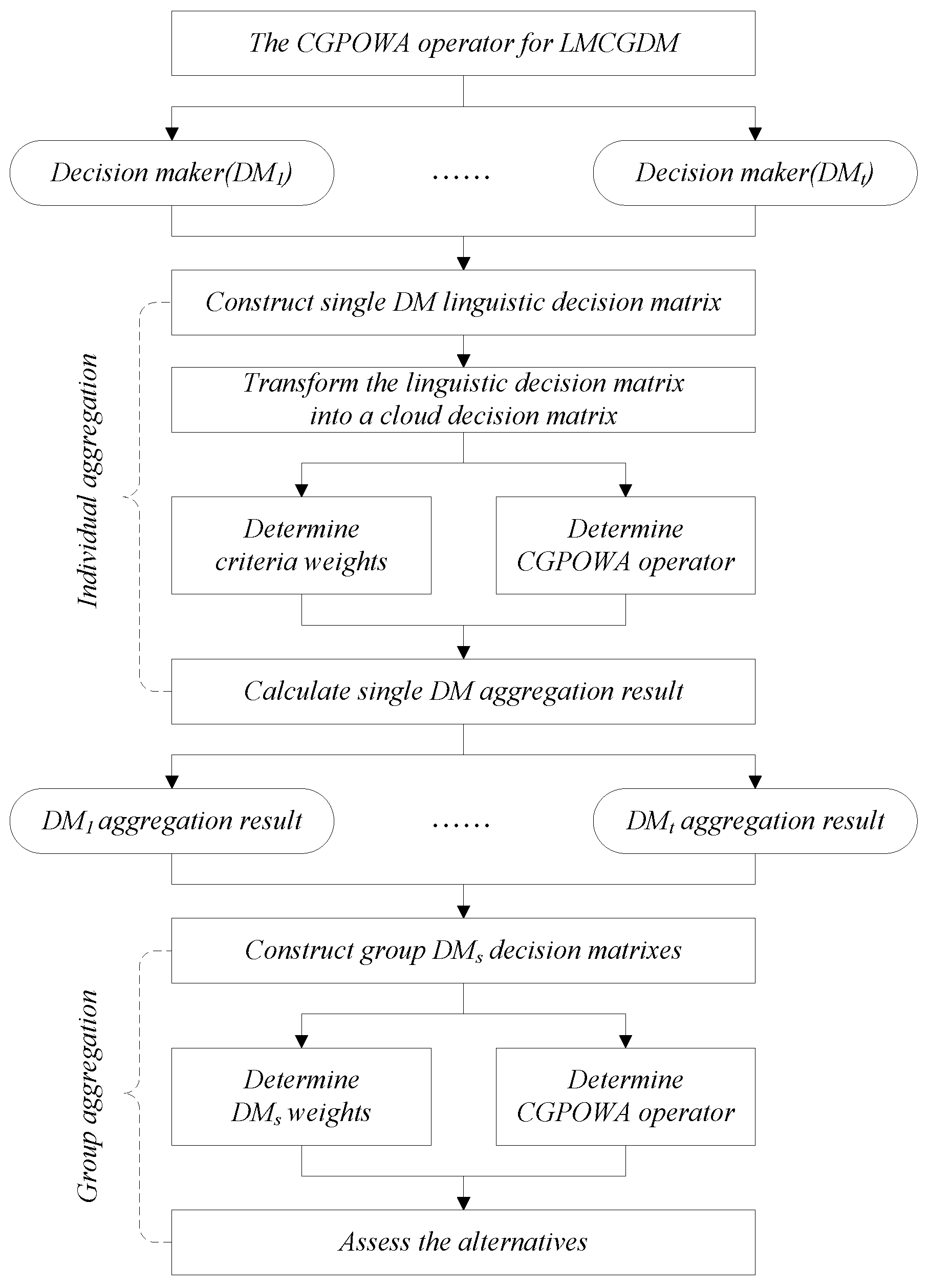
To better understand the procedure for solving LMCGDM problem on the basis of a cloud model, we develop a general framework for LMCGDM aggregation procedure (see, Figure 2) which contains two stages: (i) individual aggregation, which is a MCDM process for each DM; and (ii) group aggregation, which is a multiple experts decision-making process composed by multiple experts and multiple alternatives. For individual aggregation, we need to determine the weights of criteria, and then aggregate the criteria values of each alternative into one collective value by means of the CGPOWA operator and consequently, we derive a collective decision matrix composed by the DMs and alternatives; For group aggregation, we need to determine the weights of the DMs based on the collective decision matrix, and further aggregate the collective values of each alternative into one result by using the CGPOWA operator. Finally, we can assess the alternatives.

We develop a new algorithm for LMCGDM based on the improved generating cloud method and CGPOWA operator with the weight information being completely unknown. The algorithm is summarized in a simple algorithm through six steps. We first describe the algorithm inputs.

Input data of our new LMCGDM algorithm. Let $A=\left\{A_1,\cdots ,A_i,\cdots ,A_m\right\}$ be the set of m alternatives, $C=\left\{c_1,\cdots ,c_j,\cdots ,c_n\right\}$ be the set of n criteria, and $D=\left\{d_1,\cdots ,d_k,\cdots ,d_t\right\}$ be the set of t DMs. Assume that the DM $d_k$ provides his/her preference value ${{\tilde{b}}_{ij}}^{(k)}$ for the alternative $A_i\in A$ w. r. t. the criterion $c_j\in C$, where ${{\tilde{b}}_{ij}}^{(k)}$ takes the form of linguistic variable, and consequently we can construct a decision matrix ${\tilde{B}}^k={\left({\tilde{b}}_{ij}^{(k)}\right)}_{m\times n}$ for $d_k\in D$. We summarize all input data below:

$$\mathsf{\prod }=\left\{A,C,D,{\tilde{B}}^k\right\}$$

(17)

Given the input data $\mathsf{\prod }$ in (17), our objective is to determine the optimal alternative $A^{*}\in A$. We give a new LMCGDM approach below.

An LMCGDM algorithm.

Step 1. Transform the linguistic information into clouds.

Transform the linguistic decision matrix ${\tilde{B}}^k={\left({\tilde{b}}_{ij}^{(k)}\right)}_{m\times n}$ into a cloud decision matrix ${\widehat{R}}^k={\left({\widehat{r}}_{ij}^{(k)}\right)}_{m\times n}\left(k=1,2,\cdots ,t\right)$ by applying the improved generating cloud method developed in Section 3.

Step 2. Determine the weights of criteria.

Calculate the cloud support degrees:

$$Sup\left({\widehat{r}}_{sj}^k,{\widehat{r}}_{qj}^k\right)=1-\frac{2d\left({\widehat{r}}_{sj}^k,{\widehat{r}}_{qj}^k\right)}{{\displaystyle \sum _{\begin{array}{l}q=1\\ q\ne s\end{array}}^{n}d\left({\widehat{r}}_{sj}^k,{\widehat{r}}_{qj}^k\right)+{\displaystyle \sum _{\begin{array}{l}s=1\\ s\ne q\end{array}}^{n}d\left({\widehat{r}}_{qj}^k,{\widehat{r}}_{sj}^k\right)}}},q=1,2,\cdots ,n$$

(18)

which satisfy the support conditions (i)–(iii) in Definition 8. Here, the cloud distance measure is expressed by Equation (10), and $Sup\left({\widehat{r}}_{sj}^k,{\widehat{r}}_{qj}^k\right)$ denotes the similarity between the sth largest cloud preference value ${\widehat{r}}_{sj}^k$ and the qth largest cloud preference value ${\widehat{r}}_{qj}^k$. We further calculate the weights of criteria by means of Equation (15).

Step 3. Aggregate the criteria values of each alternative into a collective value.

Utilize Equation (14) to aggregate all cloud decision matrices ${\widehat{R}}^k={\left({\widehat{r}}_{ij}^{(k)}\right)}_{m\times n}\left(k=1,2,\cdots ,t\right)$ into a collective cloud decision matrix $R={\left(r_{ij}\right)}_{m\times t}$.

Step 4. Calculate the weights of the DMs.

Calculate the cloud support degrees:

$$Sup\left(r_{hj},r_{fj}\right)=1-\frac{2d\left(r_{hj},r_{fj}\right)}{{\displaystyle \sum _{\begin{array}{l}f=1\\ f\ne h\end{array}}^{n}d\left(r_{hj},r_{fj}\right)}+{\displaystyle \sum _{\begin{array}{l}h=1\\ h\ne f\end{array}}^{n}d\left(r_{fj},r_{hj}\right)}},f=1,2,\cdots ,t$$

(19)

which satisfy the support conditions (i)–(iii) in Definition 8. Here, the cloud distance measure is calculated by Equation (10). According to Equation (15), we can calculate the weights of the DMs.

Step 5. Aggregate the collective values of each alternative into one result.

Utilize Equation (14) to compute the collective overall preference value $r_i$ of the alternative $A_i$.

Step 6. Rank the alternatives and choose the best one(s).

According to the cloud possibility degree (11) and the ranking vector (13), we can rank the collective overall preference values $r_i(i=1,2,\cdots ,m)$ in descending order and consequently select the best one in the light of the collective overall preference values $r_i(i=1,2,\cdots ,m)$.

Remark 6.

Compared with the traditional linguistic approaches (e.g., linguistic membership function model, linguistic symbolic model, 2-tuple linguistic model) and the existing cloud aggregating method (e.g., [41]), the attractive features of our approach are as follows.

(a) 

The three traditional LMCGDM approaches only use a uniform granular linguistic assessment scale, while ours takes a multi-granular linguistic assessment scale of great psychological sense. In other words, when assessing the alternatives, these three traditional approaches only regard the average level as the unique criterion, which leads to the evaluations rough and one-sided. Our method, however, considers not only the average level but also the fluctuation and stability of qualitative concepts by using $En$ and $He$, respectively. Such statements can also be examined by the numerical analysis in Section 6.2.

(b) 

In addition, the corresponding aggregation operators for the three traditional LMCGDM methods are the linguistic power average (LPA) operator, triangular fuzzy weighted averaging (TFWA) operator and 2-tuple weighted averaging (TWA) operator, respectively. Note that these operators have their own weaknesses when describing the randomness, while our aggregation operator can effectively reduce the loss and distortion of information in aggregating process, and correspondingly improve the precision of the results.

For instance, LPA and TWA operators cannot precisely depict the randomness because when converting the linguistic variables into real numbers, they directly transform the random decision-making information into the precise domain, therefore, partial linguistic information is lost. TFWA operator can describe the fuzziness whereas it cannot describe the randomness.

(c) 

Compared with the cloud aggregating method (cf., [41]), our method provides a completely objective weighting model by using the cloud support degree, while the weights in Wang et al. [41] are subjectively given by the DMs which may result in different ranking results if the DMs provide different weight vectors. In addition, the CGPOWA operator considers the relationships between the arguments provided by the DMs, while the cloud aggregating operators in Wang et al. [41] do not.

(d) 

Our method presents a simple measure for comparing different clouds by the cloud possibility degree Equation (11) and the ranking vector Equation (13), which requires no knowledge about the distribution of cloud drops, this is different from the score function [41] which needs to know the distribution of cloud drops. This is also an attractive feature because in most case the distribution of cloud drops is unknown and it is rigid to acquire cloud drops.

6. Illustrative Example

This section provides a numerical example to illustrate the application of the approach proposed in Section 5 and makes a comparative study to examine the validity of our approach.

6.1. An Investment Selection Problem

Following [41], we assume that there is an investment company who wants to invest a sum of money in another company. There are five possible alternatives for investing the money: a car company $A_1$, a food company $A_2$, a computer company $A_3$, an arms company $A_4$, and a TV company $A_5$. The investment company will make a decision according to the following six criteria: financial risk $c_1$; technical risk $c_2$; production risk $c_3$; market risk $c_4$; management risk $c_5$; and environmental risk $c_6$. The five possible alternatives $A_i\left(i=1,\cdots ,5\right)$ are evaluated by the linguistic term set $H=\{h_{-3}=\mathrm{very}\mathrm{poor},h_{-2}=\mathrm{poor},h_{-1}=\mathrm{medium}\mathrm{poor},h_0=\mathrm{fair},h_1=\mathrm{medium}\mathrm{good},h_2=\mathrm{good},h_3=\mathrm{very}\mathrm{good}\}$ used by three DMs $d_k\left(k=1,2,3\right)$ for these six criteria. The linguistic decision matrix is shown in

Table 3. Linguistic Decision matrix $\tilde{B}$.

DMs	Alternatives	${\mathit{c}}_1$	${\mathit{c}}_2$	${\mathit{c}}_3$	${\mathit{c}}_4$	${\mathit{c}}_5$	${\mathit{c}}_6$
$d_1$	$A_1$	$h_{-1}$	$h_0$	$h_{-2}$	$h_{-2}$	$h_{-3}$	$h_{-1}$
	$A_2$	$h_{-2}$	$h_{-3}$	$h_1$	$h_1$	$h_{-2}$	$h_0$
	$A_3$	$h_2$	$h_1$	$h_2$	$h_3$	$h_0$	$h_2$
	$A_4$	$h_{-1}$	$h_{-2}$	$h_0$	$h_1$	$h_{-2}$	$h_{-1}$
	$A_5$	$h_{-1}$	$h_{-2}$	$h_0$	$h_{-2}$	$h_{-1}$	$h_2$
$d_2$	$A_1$	$h_0$	$h_{-2}$	$h_{-1}$	$h_{-1}$	$h_0$	$h_{-2}$
	$A_2$	$h_{-1}$	$h_{-2}$	$h_0$	$h_{-1}$	$h_2$	$h_0$
	$A_3$	$h_1$	$h_3$	$h_1$	$h_3$	$h_1$	$h_2$
	$A_4$	$h_{-1}$	$h_{-2}$	$h_1$	$h_{-1}$	$h_1$	$h_0$
	$A_5$	$h_3$	$h_{-3}$	$h_{-2}$	$h_0$	$h_{-1}$	$h_{-3}$
$d_3$	$A_1$	$h_1$	$h_{-1}$	$h_{-2}$	$h_0$	$h_{-3}$	$h_{-3}$
	$A_2$	$h_{-2}$	$h_1$	$h_{-1}$	$h_1$	$h_0$	$h_0$
	$A_3$	$h_2$	$h_3$	$h_1$	$h_3$	$h_1$	$h_2$
	$A_4$	$h_{-2}$	$h_2$	$h_{-1}$	$h_0$	$h_1$	$h_{-1}$
	$A_5$	$h_0$	$h_{-2}$	$h_0$	$h_{-2}$	$h_{-1}$	$h_{-3}$

.

To simplify the calculation, throughout the numerical analysis, we assume that $\phi \left(x\right)=x$, $\lambda =2$ in CGPOWA operator, and that the universe $U=[0,10]$ and $H{e}_0=0.05$ in the improved generating cloud method. Based on the approach developed in Section 5 and the given parameters, the order of enterprises can be ranked by applying MATLAB or Lingo software package.

Procedures of LMCGDM based on the cloud model.

Step 1. Transform the linguistic decision matrix into the corresponding cloud decision matrix $\widehat{R}$ by using the new cloud generating method. (See

Table 4. Cloud decision matrix $\widehat{R}$.

DMs and Alternatives		${\mathit{c}}_1$	${\mathit{c}}_2$	${\mathit{c}}_3$	${\mathit{c}}_4$	${\mathit{c}}_5$	${\mathit{c}}_6$
$d_1$	$A_1$	(4.05, 0.637, 0.08)	(5.00, 0.394, 0.05)	(3.09, 1.031, 0.13)	(3.09, 1.031, 0.13)	(0.00, 1.668, 0.21)	(4.05, 0.637, 0.08)
	$A_2$	(3.09, 1.031, 0.13)	(0.00, 1.668, 0.21)	(5.96, 0.637, 0.08)	(5.96, 0.637, 0.08)	(3.09, 1.031, 0.13)	(5.00, 0.394, 0.05)
	$A_3$	(6.93, 1.031, 0.13)	(5.96, 0.637, 0.08)	(6.93, 1.031, 0.13)	(10.0, 1.668, 0.21)	(5.00, 0.394, 0.05)	(6.93, 1.031, 0.13)
	$A_4$	(4.05, 0.637, 0.08)	(3.09, 1.031, 0.13)	(5.00, 0.394, 0.05)	(5.96, 0.637, 0.08)	(3.09, 1.031, 0.13)	(4.05, 0.637, 0.08)
	$A_5$	(4.05, 0.637, 0.08)	(3.09, 1.031, 0.13)	(5.00, 0.394, 0.05)	(3.09, 1.031, 0.13)	(4.05, 0.637, 0.08)	(6.93, 1.031, 0.13)
$d_2$	$A_1$	(5.00, 0.394, 0.05)	(3.09, 1.031, 0.13)	(4.05, 0.637, 0.08)	(4.05, 0.637, 0.08)	(5.00, 0.394, 0.05)	(3.09, 1.031, 0.13)
	$A_2$	(4.05, 0.637, 0.08)	(3.09, 1.031, 0.13)	(5.00, 0.394, 0.05)	(4.05, 0.637, 0.08)	(6.93, 1.031, 0.13)	(5.00, 0.394, 0.05)
	$A_3$	(5.96, 0.637, 0.08)	(10.0, 1.668, 0.21)	(5.96, 0.637, 0.08)	(10.0, 1.668, 0.21)	(5.96, 0.637, 0.08)	(6.93, 1.031, 0.13)
	$A_4$	(4.05, 0.637, 0.08)	(3.09, 1.031, 0.13)	(5.96, 0.637, 0.08)	(4.05, 0.637, 0.08)	(5.96, 0.637, 0.08)	(5.00, 0.394, 0.05)
	$A_5$	(10.0, 1.668, 0.21)	(0.00, 1.668, 0.21)	(3.09, 1.031, 0.13)	(5.00, 0.394, 0.05)	(4.05, 0.637, 0.08)	(0.00, 1.668, 0.21)
$d_3$	$A_1$	(5.96, 0.637, 0.08)	(4.05, 0.637, 0.08)	(3.09, 1.031, 0.13)	(5.00, 0.394, 0.05)	(0.00, 1.668, 0.21)	(0.00, 1.668, 0.21)
	$A_2$	(3.09, 1.031, 0.13)	(5.96, 0.637, 0.08)	(4.05, 0.637, 0.08)	(5.96, 0.637, 0.08)	(5.00, 0.394, 0.05)	(5.00, 0.394, 0.05)
	$A_3$	(6.93, 1.031, 0.13)	(10.0, 1.668, 0.21)	(5.96, 0.637, 0.08)	(10.0, 1.668, 0.21)	(5.96, 0.637, 0.08)	(6.93, 1.031, 0.13)
	$A_4$	(3.09, 1.031, 0.13)	(6.93, 1.031, 0.13)	(4.05, 0.637, 0.08)	(5.00, 0.394, 0.05)	(5.96, 0.637, 0.08)	(4.05, 0.637, 0.08)
	$A_5$	(5.00, 0.394, 0.05)	(3.09, 1.031, 0.13)	(5.00, 0.394, 0.05)	(3.09, 1.031, 0.13)	(4.05, 0.637, 0.08)	(0.00, 1.668, 0.21)

)

Step 2. Calculate the weights of criteria by means of Equation (15). (See

Table 5. The weights of criteria.

DMs	Alternatives	${\mathit{c}}_1$	${\mathit{c}}_2$	${\mathit{c}}_3$	${\mathit{c}}_4$	${\mathit{c}}_5$	${\mathit{c}}_6$
$d_1$	$A_1$	0.172	0.164	0.171	0.171	0.150	0.172
	$A_2$	0.170	0.154	0.168	0.168	0.170	0.171
	$A_3$	0.175	0.166	0.175	0.150	0.160	0.175
	$A_4$	0.173	0.166	0.166	0.157	0.166	0.173
	$A_5$	0.173	0.167	0.167	0.167	0.173	0.153
$d_2$	$A_1$	0.165	0.163	0.172	0.172	0.165	0.163
	$A_2$	0.172	0.160	0.172	0.172	0.153	0.172
	$A_3$	0.172	0.157	0.172	0.157	0.172	0.169
	$A_4$	0.170	0.160	0.165	0.170	0.165	0.171
	$A_5$	0.154	0.166	0.172	0.170	0.172	0.166
$d_3$	$A_1$	0.164	0.171	0.171	0.169	0.162	0.162
	$A_2$	0.155	0.167	0.164	0.167	0.173	0.173
	$A_3$	0.172	0.159	0.169	0.159	0.169	0.172
	$A_4$	0.162	0.158	0.172	0.171	0.165	0.172
	$A_5$	0.168	0.171	0.168	0.171	0.171	0.151

)

Step 3. Aggregate the criteria values of each alternative into a collective value by using Equation (14). (See

Table 6. Collective cloud decision matrix $R$.

Alternatives	$\mathbf{D}\mathbf{M}({\mathit{d}}_1)$	$\mathbf{D}\mathbf{M}({\mathit{d}}_2)$	$\mathbf{D}\mathbf{M}({\mathit{d}}_3)$
$A_1$	(3.61, 0.701, 0.09)	(4.12, 0.636, 0.09)	(3.81, 0.638, 0.08)
$A_2$	(4.41, 0.678, 0.09)	(4.81, 0.752, 0.09)	(4.97, 0.598, 0.08)
$A_3$	(7.07, 1.195, 0.15)	(7.61, 1.337, 0.17)	(7.77, 1.356, 0.17)
$A_4$	(4.31, 0.680, 0.09)	(4.80, 0.635, 0.08)	(4.99, 0.777, 0.10)
$A_5$	(4.51, 0.833, 0.11)	(4.91, 1.387, 0.17)	(3.80, 0.639, 0.08)

)

Step 4. Calculate the weights of the DMs by means of Equation (15). (See

Table 7. The weights of the DMs.

Alternatives	$\mathbf{D}\mathbf{M}({\mathit{d}}_1)$	$\mathbf{D}\mathbf{M}({\mathit{d}}_2)$	$\mathbf{D}\mathbf{M}({\mathit{d}}_3)$
$A_1$	0.330	0.307	0.363
$A_2$	0.332	0.344	0.323
$A_3$	0.289	0.364	0.346
$A_4$	0.321	0.350	0.329
$A_5$	0.361	0.298	0.341

)

Step 5. Utilize Equation (14) to compute the collective overall preference value $r_i$ of the alternative $A_i$.

$$\begin{gathered} r_1:Y_1\left(3.85,0.656,0.08\right),r_2:Y_2\left(4.73,0.679,0.09\right),r_3:Y_3\left(7.52,1.309,0.16\right), \\ {r}_4:Y_4\left(4.72,0.702,0.09\right),r_5:Y_5\left(4.41,1.037,0.13\right). \end{gathered}$$

Step 6. Rank the alternatives and choose the best one(s).

From Step 5, we can get the positive ideal cloud $Y^{*}=Y(7.52,0.656,0.08).$ Then, the ranking vector is derived by Equations (11) and (13): $V={(0.1836,0.2006,0.2216,0.2003,0.1939)}^T.$ And consequently, the rank of the clouds is: $r_3>r_4>r_2>r_5>r_1.$ The ranking order in the light of the overall collective preference values $r_i(i=1,2,3,4,5)$ is:

$$A_3\succ A_4\succ A_2\succ A_5\succ A_1.$$

Thus, the best investment alterative is the computer company $A_3$, which is in accordance with the result of Wang et al. [41]. However, compared with the cloud aggregating method, our approach has the following features:

(1)

As for the weighting method, we provide an objective weighting model based on the cloud support degree, while the weights in Wang et al. [41] are subjectively given by the DMs.

For example, Wang et al. [41] supposed that the weights of the DMs and criteria are respectively given by $\lambda ={(0.35,0.4,0.25)}^T$ and $W={(0.12,0.15,0.18,0.25,0.2,0.1)}^T$, which completely rely on the subjective preferences and knowledge of the DMs. Thus, the ranking results obtained by Wang et al. [41] are not stable because there may exist different ranking results if the DMs provide different weight vectors (See

Table 8. Ranking results for different weights of the DMs and weights of criteria.

The Weight Vector $\mathit{\lambda }$ of the DMs	The Weight Vector $\mathit{W}$ of Criteria	Ranking Results
${(0.1,0.6,0.3)}^T$	${(0.12,0.15,0.18,0.25,0.2,0.1)}^T$	$A_3\succ A_4\succ A_2\succ A_5\succ A_1$
${(0.35,0.4,0.25)}^T$	${(0.12,0.25,0.18,0.1,0.15,0.2)}^T$	$A_3\succ A_4\succ A_5\succ A_2\succ A_1$
${(0.35,0.4,0.25)}^T$	${(0.12,0.15,0.18,0.1,0.2,0.25)}^T$	$A_3\succ A_5\succ A_4\succ A_2\succ A_1$
${(0.35,0.4,0.25)}^T$	${(0.4,0.2,0.1,0.1,0.1,0.1)}^T$	$A_3\succ A_4\succ A_5\succ A_1\succ A_2$
${(0.35,0.4,0.25)}^T$	${(0.2,0.4,0.1,0.1,0.1,0.1)}^T$	$A_3\succ A_4\succ A_1\succ A_5\succ A_2$
${(0.35,0.4,0.25)}^T$	${(0.2,0.1,0.1,0.1,0.1,0.4)}^T$	$A_3\succ A_5\succ A_2\succ A_4\succ A_1$

). However, our method does not require the DMs to provide weighting information and the weights are derived based on the objective data and the cloud support degree Equation (15), and then the ranking results generally remain unchanged (See

Table 9. Comparison with different parameter $\lambda$.

Aggregation Operators	Ranking Vector	Ranking Results
CGPOWA $(\lambda =1)$	${(0.1769,0.1962,0.2468,0.1977,0.1824)}^T.$	$A_3\succ A_4\succ A_2\succ A_5\succ A_1$
CGPOWA $(\lambda =2)$	${(0.1836,0.2003,0.2216,0.2006,0.1939)}^T.$	$A_3\succ A_4\succ A_2\succ A_5\succ A_1$
CGPOWA $(\lambda =3)$	${(0.1872,0.2021,0.2052,0.2034,0.2020)}^T.$	$A_3\succ A_4\succ A_2\succ A_5\succ A_1$

).

(2)

Our method considers the relationship between arguments given by the DMs, while Wang et al. [41] neglect it.

For instance, CWAA and CWGA operators provided by Wang et al. [41] do not consider the relationship between the arguments, while the CGPOWA operator we derived considers the relationship among input arguments by allowing values being aggregated to support and reinforce each other via cloud support degrees. Here, cloud support degrees of the arguments can be calculated by applying Equations (18) and (19).

6.2. Comparative Analysis

To validate the feasibility of our method, a comparative study is conducted by applying three traditional LMCGDM methods, i.e., linguistic symbolic model, linguistic membership function model, 2-tuple linguistic model. The corresponding aggregation operators for the three traditional LMCGDM methods are respectively the LPA operator, TFWA operator and TWA operator. This comparative analysis is based on the same illustrative example given in Section 6.1. The weights of the DMs and criteria are respectively taken from Table 4 and Table 6 so as to make it easy to compare these results with the case of our method.

• Linguistic symbolic model

First, aggregate all linguistic decision matrices ${\tilde{B}}^{(k)}={\left({\tilde{b}}_{ij}^{(k)}\right)}_{5\times 6}$ into a collective linguistic decision matrix $B={\left(b_{ij}\right)}_{5\times 6}$ by applying LPA operator (See

Table 10. Collective linguistic decision matrix $B.$

Alternatives	${\mathit{c}}_1$	${\mathit{c}}_2$	${\mathit{c}}_3$	${\mathit{c}}_4$	${\mathit{c}}_5$	${\mathit{c}}_6$
$A_1$	$h_0$	$h_{-1}$	$h_{-1.736}$	$h_{-1}$	$h_{-2.208}$	$h_{-2}$
$A_2$	$h_{-1.736}$	$h_{-1.388}$	$h_0$	$h_{0.276}$	$h_0$	$h_0$
$A_3$	$h_{1.736}$	$h_{2.472}$	$h_{1.264}$	$h_3$	$h_{0.736}$	$h_2$
$A_4$	$h_{-1.264}$	$h_{-0.944}$	$h_0$	$h_0$	$h_{0.208}$	$h_{-0.736}$
$A_5$	$h_{0.529}$	$h_{-2.264}$	$h_{-0.528}$	$h_{-0.736}$	$h_{-1}$	$h_{-1.68}$

).

Second, utilize LPA operator to derive the overall collective preference values.

$$t_1:h_{-1.328},t_2:h_{-0.453},t_3:h_{1.868},t_4:h_{-0.455},t_5:h_{-0.948}.$$

Finally, rank the order of the five alternatives: $A_3\succ A_2\succ A_4\succ A_5\succ A_1.$

• Linguistic membership function model

First, transform linguistic variables into triangular fuzzy numbers by the method of Iraj et al. [47]:

$$h_3:\left(9,10,10\right),h_2:\left(7,9,10\right),h_1:\left(5,7,9\right),h_0:\left(3,5,7\right),h_{-1}:\left(1,3,5\right),h_{-2}:\left(0,1,3\right),h_{-3}:\left(0,0,1\right).$$

Second, utilize TFWA operator to derive the individual overall evaluation value $T_i^k$:

$$\begin{gathered} T_1^1=\left(0.67,1.84,3.64\right),T_1^2=\left(1.39,3.14,5.14\right),T_1^3=\left(1.50,2.72,4.42\right), \\ {T}_2^1=\left(2.45,3.83,5.68\right)T_2^2=\left(2.61,4.46,6.26\right)T_2^3=\left(2.90,4.60,6.60\right), \\ {T}_3^1=\left(6.40,8.15,9.25\right),T_3^2=\left(6.80,8.40,9.50\right)T_3^3=\left(7.04,8.64,9.62\right), \\ {T}_4^1=\left(2.01,3.66,5.66\right),T_4^2=\left(2.57,4.42,6.42\right),T_4^3=\left(3.08,4.96,6.81\right), \\ {T}_5^1=\left(1.56,3.16,5.06\right),T_5^2=\left(2.03,3.23,4.74\right),T_5^3=\left(1.10,2.50,4.40\right). \end{gathered}$$

Third, use TFWA operator to determine the overall collective evaluation value ${\dot{T}}_i$:

$$\begin{gathered} {\dot{T}}_1=\left(1.17,2.58,4.44\right),{\dot{T}}_2=\left(2.63,4.27,6.14\right),{\dot{T}}_3=\left(6.72,8.37,9.44\right), \\ {\dot{T}}_4=\left(2.50,4.23,6.25\right),{\dot{T}}_5=\left(1.63,3.02,4.77\right). \end{gathered}$$

Finally, rank the order of the five alternatives via the method of comparing triangular fuzzy numbers (Chang & Wang, [48]): $A_3\succ A_2\succ A_4\succ A_5\succ A_1.$

• 2-tuple linguistic model

First, utilize TWA operator to derive the individual overall evaluation value:

$$\begin{gathered} S_1^1=\left(-2,0.32\right),S_2^1=\left(-1,0.34\right),S_3^1=\left(2,-0.3\right),S_4^1=\left(-1,0.33\right),S_5^1=\left(-1,0.08\right), \\ {S}_1^2=\left(-1,0.07\right),S_2^2=\left(0,-0.27\right),S_3^2=\left(2,-0.1\right),S_4^2=\left(0,-0.29\right),S_5^2=\left(-1,0.05\right), \\ {S}_1^3=\left(-1,-0.29\right),S_2^3=\left(0,-0.02\right),S_3^3=\left(2,0.02\right),S_4^3=\left(0,0.02\right),S_5^3=\left(-1,-0.3\right). \end{gathered}$$

Second, apply TWA operator to get the overall collective evaluation values ${\dot{S}}_i$:

$${\dot{S}}_1=\left(-1,-0.283\right),{\dot{S}}_2=\left(0,-0.344\right),{\dot{S}}_3=\left(2,-0.14\right),{\dot{S}}_4=\left(0,-0.356\right),{\dot{S}}_1=\left(-1,-0.027\right).$$

Third, rank the order of the five alternatives: $A_3\succ A_2\succ A_4\succ A_5\succ A_1.$

Table 11. Comparison with different models.

Aggregation Operators	Ranking Results
LPA	$A_3\succ A_2\succ A_4\succ A_5\succ A_1$
TFWA	$A_3\succ A_2\succ A_4\succ A_5\succ A_1$
TWA	$A_3\succ A_2\succ A_4\succ A_5\succ A_1$

shows the ranking results with three different aggregation operators (i.e., LPA, TFWA, TWA). Comparing Table 11 with Table 9, we find that the respective ranking results of the three operators are all the same, but the ranking result is different when the CGPOWA operator is applied. The difference lies in the ranking order of $A_2$ and $A_4$.

The above difference can be explained by the following fact: when the alternatives are assessed, these three traditional methods only regard the average level as the unique criterion, which leads to the evaluations rough and one-sided. Notice that the average level of $A_2$ is higher than the case of $A_4$, and then the ranking order of these three traditional methods becomes $A_2\succ A_4$. Our method, however, considers not only the average level but also the fluctuation and stability of qualitative concepts by using $En$ and $He$, respectively. In other words, the three traditional methods only use a uniform granular linguistic assessment scale, while our method takes a multi-granular linguistic assessment scale of great psychological sense. This causes the average level of $A_2$ to be lower than the case of $A_4$, namely, $E{x}_2<E{x}_4$. In addition, we derive that $E{n}_2>E{n}_4$ and $H{e}_2>H{e}_4$ in this example. Therefore, according to Equation (13), we can conclude that the ranking result becomes $A_4\succ A_2$ in our method.

7. Conclusions

LMCDM problems are widespread in various fields such as economics, management, medical care, social sciences, engineering, and military applications. However, traditional aggregation methods are not robust enough to convert qualitative concepts to quantitative information in LMCDM problems. Among the existing aggregation operators, linguistic power aggregation operators and cloud aggregation operators have the most merits, but they have their own weaknesses. If combined together, the two types of operators can overcome their own weaknesses, that is, the characters of two types of operators are mutually complementary. This paper developed a new class of aggregation operator which successfully unified the advantages of the existing linguistic power aggregation operators and cloud aggregation operators, and simultaneously overcame their limitations. First, we presented an improved method to transform linguistic variables into clouds, which corrects the weaknesses of the classical generating cloud method. Based on this method, we developed some new cloud algorithms such as the cloud possibility degree and cloud support degree, which can be used for cloud comparison and the weight determination, respectively. Furthermore, a new CGPOWA operator was developed, which considers the decision arguments and their relationships and characterizes the fuzziness and randomness of linguistic terms. By studying the properties of CGPOWA operator we found that it is commutative, idempotent, bounded. Moreover, CGPOWA operator can degenerate into many different operators, including CGPA operator, CPOWA operator, CPOWGA operator, CPWQA operator, CWAA and CWGA operators, the maximum operator and the minimum operator. In particular, based on the new generating cloud method and CGPOWA operator, a new approach for LGDM was developed. In the end, to show the effectiveness and the good performance of our approach in practice, we provided an example of investment selection and made a comparative analysis.

In further research, it would be very interesting to extend our analysis to the case of more sophisticated situation such as introducing the behavior theory of the DMs in the context of CGOWPA operator. Nevertheless, we leave that point to future research, since our methodology cannot be applied to that extended framework, which will result in more sophisticated calculation and which we cannot tackle here.

References

- Wiecek, M.M.; Ehrgott, M.; Fadel, G.; Figueira, J.R. Multiple criteria decision-making for engineering. Omega 2008, 36, 337–339. [Google Scholar] [CrossRef]
- Wu, J.; Li, J.C.; Li, H.; Duan, W.Q. The induced continuous ordered weighted geometric operators and their application in group decision-making. Comput. Ind. Eng. 2009, 58, 1545–1552. [Google Scholar] [CrossRef]
- Xia, M.M.; Xu, Z.S. Methods for fuzzy complementary preference relations based on multiplicative consistency. Comput. Ind. Eng. 2011, 61, 930–935. [Google Scholar] [CrossRef]
- Merigó, J.M.; Casanovas, M. Induced and uncertain heavy OWA operators. Comput. Ind. Eng. 2011, 60, 106–116. [Google Scholar] [CrossRef]
- Gong, Y.B.; Hu, N.; Zhang, J.G.; Liu, G.F.; Deng, J.G. Multi-attribute group decision-making method based on geometric Bonferroni mean operator of trapezoidal interval type-2 fuzzy numbers. Comput. Ind. Eng. 2015, 81, 167–176. [Google Scholar] [CrossRef]
- Wan, S.P.; Wang, F.; Lin, L.L.; Dong, J.Y. Some new generalized aggregation operators for triangular intuitionistic fuzzy numbers and application to multi-attribute group decision-making. Comput. Ind. Eng. 2016, 93, 286–301. [Google Scholar] [CrossRef]
- Ngan, S.C. A type-2 linguistic set theory and its application to multi-criteria decision-making. Comput. Ind. Eng. 2013, 64, 721–730. [Google Scholar] [CrossRef]
- Wei, G.W.; Zhao, X.F.; Lin, R. Some hybrid aggregating operators in linguistic decision-making with Dempster-Shafer belief structure. Comput. Ind. Eng. 2013, 65, 646–651. [Google Scholar] [CrossRef]
- Wang, Z.Q.; Richard, Y.K.F.; Li, Y.L.; Pu, Y. A group multi-granularity linguistic-based methodology for prioritizing engineering characteristics under uncertainties. Comput. Ind. Eng. 2016, 91, 178–187. [Google Scholar] [CrossRef]
- Yager, R.R. Fusion of ordinal information using weighted median aggregation. Int. J. Approx. Reason. 1998, 18, 35–52. [Google Scholar] [CrossRef]
- Xu, Z.S. An overview of operators for aggregating information. Int. J. Intell. Syst. 2003, 18, 953–969. [Google Scholar] [CrossRef]
- Xu, Z.S. Deviation measures of linguistic preference relations in group decision-making. Omega 2005, 33, 249–254. [Google Scholar] [CrossRef]
- Yager, R.R. An approach to ordinal decision-making. Int. J. Approx. Reason. 1995, 12, 237–261. [Google Scholar] [CrossRef]
- Yager, R.R.; Rybalov, A. Understanding the median as a fusion operator. Int. J. Gen. Syst. 1997, 26, 239–263. [Google Scholar] [CrossRef]
- Yager, R.R. Applications and extensions of OWA aggregations. Int. J. Man-Mach. Stud. 1992, 37, 103–132. [Google Scholar] [CrossRef]
- Herrera, F.; Herrera-Viedma, E. Aggregation operators for linguistic weighted information. IEEE Trans. Syst. Man Cybern. Part A 1997, 27, 646–656. [Google Scholar] [CrossRef]
- Lee, H.M. Applying fuzzy set theory to evaluate the rate of aggregative risk in software development. Fuzzy Sets Syst. 1996, 79, 323–336. [Google Scholar] [CrossRef]
- Lee, H.M.; Lee, S.Y.; Lee, T.Y.; Chen, J.J. A new algorithm for applying fuzzy set theory to evaluate the rate of aggregative risk in software development. Inf. Sci. 2003, 153, 177–197. [Google Scholar] [CrossRef]
- Herrera, F.; Herrera-Viedma, E.; Verdegay, J.L. A sequential selection process in group decision-making with a linguistic assessment approach. Inf. Sci. 1995, 85, 223–239. [Google Scholar] [CrossRef]
- Torra, V. The weighted OWA operator. Int. J. Intell. Syst. 1997, 12, 153–166. [Google Scholar] [CrossRef]
- Herrera, F.; Herrera-Viedma, E. Linguistic decision analysis: Steps for solving decision problems under linguistic information. Fuzzy Sets Syst. 2000, 115, 67–82. [Google Scholar] [CrossRef]
- Merigó, J.M.; Casanovas, M. Decision-making with distance measures and linguistic aggregation operators. Int. J. Fuzzy Syst. 2010, 12, 190–198. [Google Scholar]
- Zhou, L.G.; Chen, H.Y. The induced linguistic continuous ordered weighted geometric operator and its application to group decision-making. Comput. Ind. Eng. 2013, 66, 222–232. [Google Scholar] [CrossRef]
- Zhou, L.; Wu, J.; Chen, H.Y. Linguistic continuous ordered weighted distance measure and its application to multiple attributes group decision-making. Appl. Soft Comput. 2014, 25, 266–276. [Google Scholar] [CrossRef]
- Merigó, J.M.; Palacios-Marqué, D.; Zeng, S.Z. Subjective and objective information in linguistic multi-criteria group decision-making. Eur. J. Oper. Res. 2016, 248, 522–531. [Google Scholar] [CrossRef]
- Herrera, F.; Martínez, L. A model based on linguistic 2-tuples for dealing with multi granular hierarchical linguistic contexts in multi-expert decision-making. IEEE Trans. Syst. Man Cybern. Part B 2001, 31, 227–234. [Google Scholar] [CrossRef] [PubMed]
- Herrera, F.; Martinez, L. A 2-tuple fuzzy linguistic representation model for computing with words. IEEE Trans. Fuzzy Syst. 2015, 8, 746–752. [Google Scholar]
- Wei, G.; Zhao, X. Some dependent aggregation operators with 2-tuple linguistic information and their application to multiple attribute group decision-making. Expert Syst. Appl. 2012, 39, 5881–5886. [Google Scholar] [CrossRef]
- Wan, S.P. 2-Tuple linguistic hybrid arithmetic aggregation operators and application to multi-attribute group decision-making. Knowl.-Based Syst. 2013, 45, 31–40. [Google Scholar] [CrossRef]
- Xu, Z.S. On generalized induced linguistic aggregation operators. Int. J. Gen. Syst. 2006, 35, 17–28. [Google Scholar] [CrossRef]
- Xu, Z.S. EOWA and EOWG operators for aggregating linguistic labels based on linguistic preference relations. Int. J. Uncertain. Fuzziness Knowl.-Based Syst. 2004, 12, 791–810. [Google Scholar] [CrossRef]
- Xu, Y.J.; Da, Q.L. Standard and mean deviation methods for linguistic group decision-making and their applications. Expert Syst. Appl. 2010, 37, 5905–5912. [Google Scholar] [CrossRef]
- Xu, Z.S. A method based on linguistic aggregation operators for group decision-making with linguistic preference relations. Inf. Sci. 2004, 166, 19–30. [Google Scholar] [CrossRef]
- Xu, Y.J.; Da, Q.L.; Zhao, C.X. Interactive approach for multiple attribute decision-making with incomplete weight information under uncertain linguistic environment. Syst. Eng. Electron. 2009, 31, 597–601. [Google Scholar]
- Xu, Z.S. Induced uncertain linguistic OWA operators applied to group decision-making. Inf. Fusion 2006, 7, 231–238. [Google Scholar] [CrossRef]
- Xu, Z.S. An approach based on the uncertain LOWG and induced uncertain LOWG operators to group decision-making with uncertain multiplicative linguistic preference relations. Decis. Support Syst. 2006, 41, 488–499. [Google Scholar] [CrossRef]
- Yager, R.R. The power average operator. IEEE Trans. Syst. Man Cybern. Part A 2001, 31, 724–731. [Google Scholar] [CrossRef]
- Xu, Y.; Merigó, J.M.; Wang, H. Linguistic power aggregation operators and their application to multiple attribute group decision-making. Appl. Math. Model. 2012, 36, 5427–5444. [Google Scholar] [CrossRef]
- Zhou, L.; Chen, H.Y. A generalization of the power aggregation operators for linguistic environment and its application in group decision-making. Knowl.-Based Syst. 2012, 26, 216–224. [Google Scholar] [CrossRef]
- Li, D.; Meng, H.; Shi, X. Membership clouds and membership cloud generators. J. Comput. Res. Dev. 1995, 32, 16–21. [Google Scholar]
- Wang, J.Q.; Peng, L.; Zhang, H.Y.; Chen, X.H. Method of multi-criteria group decision-making based on cloud aggregation operators with linguistic information. Inf. Sci. 2014, 274, 177–191. [Google Scholar] [CrossRef]
- Wang, J.Q.; Wang, P.; Wang, J.; Zhang, H.Y.; Chen, X.H. Atanassov’s interval-valued intuitionistic linguistic multi-criteria group decision-making method based on trapezium cloud model. IEEE Trans. Fuzzy Syst. 2015, 23, 542–554. [Google Scholar] [CrossRef]
- Li, D.Y.; Du, Y. Artificial Intelligence with Uncertainty; Chapman & Hall/CRC, Press: Boca Raton, FL, USA, 2007. [Google Scholar]
- Li, D.Y.; Liu, C.Y.; Gan, W.Y. A new cognitive model: Cloud model. Int. J. Intell. Syst. 2009, 24, 357–375. [Google Scholar] [CrossRef]
- Wang, H.L.; Feng, Y.Q. On multiple attribute group decision-making with linguistic assessment information based on cloud model. Control Decis. 2005, 20, 679–685. [Google Scholar]
- Wan, S.P.; Dong, J.Y. A possibility degree method for interval-valued intuitionistic fuzzy multi-attribute group decision-making. J. Comput. Syst. Sci. 2014, 80, 237–256. [Google Scholar] [CrossRef]
- Iraj, M.; Nezam, M.A.; Armaghan, H.; Rahele, N. Designing a model of fuzzy TOPSIS in multiple criteria decision-making. Appl. Math. Comput. 2008, 206, 607–617. [Google Scholar]
- Chang, T.H.; Wang, T.C. Using the fuzzy multi-criteria decision-making approach for measuring the possibility of successful knowledge management. Inf. Sci. 2009, 179, 355–370. [Google Scholar] [CrossRef]
Figure 1.
Cloud (50, 3.93, 0.1).
Figure 2.
General Framework of the CGPOWA Operator for an LMCGDM Procedure.