Local-Basis-Function Equation of State for Ice VII–X to 450 GPa at 300 K

Abstract

Helmholtz energy of ice VII–X is determined in a pressure regime extending to 450 GPa at 300 K using local-basis-functions in the form of b-splines. The new representation for the equation of state is embedded in a physics-based inverse theory framework of parameter estimation. Selected pressures as a function of volume from 14 prior experimental studies and two theoretical studies constrain the behavior of Helmholtz energy. Separately measured bulk moduli, not used to construct the representation, are accurately replicated below about 20 GPa and above 60 GPa. In the intermediate range of pressure, the experimentally determined moduli are larger and have greater scatter than values predicted using the Helmholtz representation. Although systematic error in the determination of elastic moduli is possible and likely, the alternative hypothesis is a slow relaxation time associated with changes in proton mobility or the ice VII to X transition. A correlation is observed between anomalies in the pressure derivative of the predicted bulk modulus and previously suggested higher-order phase transitions. Improved determinations of elastic properties at high pressure would allow refinement of the current equation of state. More generally, the current method of data assimilation is broadly applicable to other materials in high-pressure studies and for investigations of planetary interiors.

1. Introduction

From icy worlds of our solar system to water-rich super-Earth exoplanets, high-pressure water ices are potential planetary constituents that can exist as distinct mineral species. For example, on Earth, ice VII as a mineral inclusion has been identified in a mantle-derived diamond [1]. Having an accurate equation of state representations for all ice phases is a prerequisite in evaluating questions of origins, evolution, and the potential habitability of ocean worlds [2,3,4,5,6,7,8,9]. A particularly challenging domain for equation of state analysis of ices lies between 2.2 GPa (the pressure of the first order transition between tetragonal ice VI and cubic ice VII) and 450 GPa where three-fold compression is accommodated without first order transitions. First order transitions have been predicted to occur in a regime beyond 300–400 GPa. The experimental and theoretical evidence for higher order transitions at lower pressures is further discussed below.

To provide an improved representation of ice, a new framework for equations of state analysis is described that relies on the thermodynamic representation of Helmholtz energy. The approach follows naturally from long-standing ideas. Birch [10] identified four principle means to obtain equation of state representations: (1) quantum-mechanical treatment, (2) the Thomas–Fermi electron gas approximation, (3) semi-empirical laws for interactions of atoms and ions, and (4) thermodynamic relationships involving elasticity. The latter, a thermodynamic approach using a series of expansions truncated at a low order of Helmholtz energy with parameters expressed in terms of the bulk modulus and its first two pressure derivatives, is the widely practiced approach. This approach can, in addition, be related to special cases of semi-empirical laws for atom/ion interactions [11]. Here, results from quantum mechanical and Thomas–Fermi calculations are combined with measurements within the new framework.

The current work is also guided by the Stacey et al. [11] comments that “Since almost any analytic form may be used to represent a finite data set if sufficient arbitrary or adjustable constants are allowed, we may logically regard as most successful those that use fewest such constants to achieve a particular precision of fit. If this still leaves too much choice, we would prefer a theory in which the adjustable constants are determined most directly from observations.” The new framework is responsive to the need to keep the size (number of required parameters) of a model small, while adequately representing measurements, theory, and physical insight garnered from examination of data and calculations. An additional argument developed here is that representational results should not depend on the method of parameterization (i.e., the choice of underlying basis functions) and the size of a model should be flexibly adjusted to meet the physics needs of a particular material.

Our primary findings are straightforward. The traditional physics-blind series expansion to low order of Helmholtz energy, while successful in reproducing measurements and/or theory in restricted regimes of compression, eventually fails over larger regimes. Electronic states and the nature of bonding fundamentally change over a large range of compression. Representations, as developed here, preserve the concept of low-order expansions, using subdomains of compression, while allowing for the necessary changes of the crystal potential (as represented by Helmholtz energy) over larger regimes of pressure and volume compression. Within this framework, concerns that dominate conventional equation of state analysis, including the choice of the expansion order and the definition of a strain metric, become less important. The relevant concerns then appropriately shift to a physics-based discussion: the relative weighting of data from varied sources, the quality of results based on theory, as well as the articulation of appropriate physical insight that should be applied to the representations.

In the following sections we (1) review knowledge concerning the behavior of ice beyond 2.2 GPa, (2) discuss the conceptual foundations of conventional equations of state based on series expansions of Helmholtz energy in powers of strain, (3) describe local-basis-functions that are related to, but more flexible than the polynomial global-basis-functions underlying standard parameterizations, (4) test the new framework against data over an extended regime of pressure for a relatively simple ionic material (NaCl), and finally, (5) use the new framework in analysis of high pressure ices. Mathematical and conceptual details of the framework are given in an exposition on basis functions and inverse theory found in Appendix A.

Phase Behavior of Ice Beyond 2.2 GPa

Although continuous in volume, the complex variations in observed physical properties in the stability field of ice VII and ice X are currently understood as changes in proton dynamics and distortions of the oxygen lattice during compression. Details of transitions remain debated and observations that support the existence of higher-order transitions are summarized in

Table 1. Reported transitions in ice VII and ice X.

Pressure of Transition	Suggested Transition	Type of Measurements	References
5 GPa
5 GPa	Tetragonal distortion	Powder X-Ray diffraction (XRD)	Grande et al. [21]
10–15 GPa
11 GPa	Lattice distortion	XRD peak splitting	Hirai et al. [22]
14 GPa	Strain in cubic lattice	Powder X-Ray diffraction	Somayazulu et al. [23]
11 GPa	-	Changes in Raman line width trends for the ${\nu }_1\left(A_{1g}\right)$ band	Hirai et al. [22], Pruzan et al. [24]
13–15 GPa	-	Raman line pressure trends	Zha et al. [25]
13 GPa	-	Neutron diffraction (220/110 ratio)	Guthrie et al. [26]
10–14 GPa	Lattice distortion	c/a ratio changes in ice VIII	Yoshimura et al. [27]
10–14 GPa	-	Maximum in electrical conductivity	Okada et al. [28]
10–15 GPa	-	Maximum in proton diffusion	Noguchi et al. [29]
20–25 GPa—Possible transition to Ice VII’ with proton dynamic disorder (tunneling and thermal hoping)
23–25 GPa	-	Bump in the 220/110 ratio from Neutron diffraction	Guthrie et al. [26]
25 GPa	Proton tunneling: ice VII’	IR reflectivity trend of ${\nu }_3$ and ${\nu }_3\prime$ trend	Goncharov et al. [18]
20–25 GPa	Proton tunneling: ice VII’	H-NMR	Meier et al. [20]
27 GPa	-	Raman line pressure trends	Zha et al. [25]
40 GPa
40 GPa	Softening	Drop in volume reported based on XRD	Hemley et al. [15], Loubeyre et al. [16], Sugimura et al. [17]
44 GPa	-	Raman line pressure trends	Zha et al. [25]
44 GPa	-	Discontinuity in the pressure dependence of Brillouin esound speeds	Noguchi et al. [30]
40 Gpa	-	Changes in trend of reflective index	Zha et al. [19]
40 GPa	-	Drop in Brillouin transverse wave speeds over a narrow P range (<2 GPa) in compression and decompression	Asahara et al. [31]
>60 GPa transition to ice X
60 GPa	Proton symmetrization	IR reflectivity trend of ${\nu }_3\prime$ and translation modes ${\nu }_T$	Goncharov et al. [18]
62 GPa	-	Raman line pressure trends	Zha et al. [25]
60 Gpa	-	Changes in trend of reflective index	Zha et al. [19]
59 GPa	-	Drop in Brillouin transverse wave speeds in compression	Asahara et al. [31]
70 GPa	Proton symmetrization	H-NMR	Meier et al. [20]
90 GPa	Proton symmetrization	Emergence of the p20 Raman mode	Zha et al. [25]

and are further discussed here. International Union of Crystallography “short name” designations are used to describe the space group of ice phases in the following discussion.

Cubic ice VII (Pn-3m) is stable beyond 2.2 GPa until reaching an indistinct transition above about 60 GPa to ice X. The gradual symmetrization of hydrogens between oxygens leads to ionic ice X (which is also Pn-3m). The stability of cubic ice X above 150 GPa is experimentally unconstrained, but density-functional calculations of ground state structures [12,13] suggest an eventual transition to the Pbcm structure between 300–400 GPa, then to Pmc2₁ at 930 GPa and P2₁ at 1.3 TPa. Eventually a metallic transition to C2/m is predicted at 4.8 TPa. At higher temperatures, ice X transforms into super-ionic ice XVIII above 2000 K [14]. At pressures below 100 GPa, anomalies are reported associated with changes in derivatives or discontinuities in optical spectra, bulk moduli, proton dynamics, and electrical conductivity. The most prominent features include a suggested softening of ice VII volume around 40 GPa [15,16,17] and the onset of the ice X transition by proton symmetrization above about 65 GPa. The latter is supported by changes in the IR reflectivity trend of ν₃’ and translation modes ν_Τ [18], optical reflectivity [19] and from H-NMR experiments [20].

Several other potential higher order transitions have been identified. Tetragonal distortion is possible above 5 GPa [21]. Between 10 GPa and 14 GPa shifts are observed in X-Ray, Neutron, and Raman measurements [22,23,24,26]. Such behavior is also observed in the proton-ordered analog of ice VII, known as ice VIII [27]. The initiation of proton tunneling above 25 GPa (possible transition to ice VII’) is interpreted on the basis of IR reflectometry [18] and H-NMR data [20].

Equations of state for ice VII and X based on density functional theory, developed by French et al. [32], show variable degrees of agreement with measurements at 295 K depending on the chosen potential and the range of density. They noted that “the fitting of experimental data for such a complex solid may require using a more refined parametric equation of state than the simple Vinet formula, even when the equation of state is split into multiple sections [33]”.

As a result of the complex behavior noted here, ice VII and X viewed as a single-phase continuum, cannot be appropriately represented by a single (relatively low order) global polynomial-based equation of state. Previous equations of state, constrained by measurements over limited and differing ranges, present a confusing collection of parameterizations. Extrapolations using any of these equations of states to higher or to lower pressures than the range of fitted data results in significant misfits of other measurements.

2. Materials and Methods

2.1. Helmholtz Energy-Based Equations of State

Here, a brief overview of conventional (global) equation of state parameterizations is provided to differentiate them from the local-basis-function method described later. The derivation of an equation of state based on a series expansion of Helmholtz energy as a function of a strain metric, η, has been extensively discussed [10,11,34,35,36]. The choice of strain metric is arbitrary, and several have found favor in successful applications of data representation, although the finite strain metric based on an Eulerian representation (as opposed to Lagrangian) is commonly adopted. The Eulerian finite strain metric (as used in the Birch–Murnaghan equation of state) is $\eta =1/2({(V/V_o)}^{-2/3}-1)$, where V is volume and subscript refers to the ambient pressure value. The Vinet strain metric [36] is $\eta =({(V/V_o)}^{-1/3}-1)$. Poirier and Tarantola [35] developed a logarithmic equation of state using $\eta =-1/2\log (V/V_o)$. Other definitions are possible and have been used.

The expansion of the Helmholtz energy about ambient pressure as a function of the strain metric is given as

$$F\left(\eta \right)=F_o+F_1{\eta }^1+F_2{\eta }^2+F_3{\eta }^3+F_4{\eta }^4+\dots$$

(1)

where the expansion coefficients F_i contain appropriate derivatives of F evaluated at η = 0. The first term on the right establishes the energy datum. Pressure follows as

$$P\left(V\right)=-\frac{dF}{dV}=-\frac{dF}{d\eta }\frac{d\eta }{dV}=\frac{d\eta }{dV}\left(F_1+2F_2\eta +3F_3{\eta }^2+4F_4{\eta }^3+\dots \right)$$

(2)

The $F_1$ term is conventionally set to zero, although more formally Equation (2) should predict ambient pressure (0.1 MPa) for η = 0. The isothermal bulk modulus given as

$$K=-V\frac{dP}{dV}$$

(3)

has pressure derivatives indicated by the number of prime superscripts:

$$K^{\prime }=\frac{dK}{dP}K″=\frac{d^{2}K}{d{P}^2}K‴=\frac{d^{3}K}{d{P}^3}.$$

Based on one definition for strain, the Eulerian strain metric, and with algebraic effort, Equation (2), truncated at the fourth order in energy, can be expressed in terms of the ambient pressure bulk modulus and its pressure derivatives (denoted with subscript) as:

$$P=\frac{9K_o}{16}\left(-B_1{\left(\frac{V}{V_o}\right)}^{-5/3}+B_2{\left(\frac{V}{V_o}\right)}^{-7/3}-B_3{\left(\frac{V}{V_o}\right)}^{-9/3}+B_4{\left(\frac{V}{V_o}\right)}^{-11/3}\right)$$

(4)

$$B_1=K_o{K}_o^{"}+(K_o^{\prime }-4)(K_o^{\prime }-5)+59/9,$$

$$B_2=3K_o{K}_o^{"}+(K_o^{\prime }-4)(3K_o^{\prime }-13)+129/9,$$

$$B_3=3K_o{K}_o^{"}+(K_o^{\prime }-4)(3K_o^{\prime }-11)+105/9,$$

$$B_4=K_o{K}_o^{"}+(K_o^{\prime }-4)(K_o^{\prime }-3)+39/9.$$

Equations (2) and (4) contain the common physical assumption that a low order series expansion of energy is adequate. The focus in Equation (2) is on model parameters that are measures of derivatives of the energy at equilibrium. In Equation (4), with application of a particular strain metric, parameters are cast as elastic properties determined at ambient condition. The use of other strain metrics generates different algebraic relationships but preserves the underlying physics of a truncated series expansion.

While expansion of Equation (1) to arbitrary higher order is straightforward, equation of state applications have been limited to no more than fourth-degree polynomials for several reasons. A general belief has been that an appropriate choice of a strain might lead naturally to a convergent series. Higher order derivatives of the bulk modulus are not well constrained by pressure–volume measurements that may not be sufficiently accurate and/or span a sufficiently large range of compression. The low order (second and third) forms of Equation (4) have provided relatively stable extrapolations to high pressure and have proven adequate to represent many measurements. The fourth-order expansion is often marginally stable or completely unstable in extrapolation. Higher order versions fit to measurements are expected to be less stable. The algebraic and arithmetic effort to relate the energy expansion coefficients to derivatives of the bulk modulus increases with increasing order.

The strength of the strain-expansion-based representation of data is that a small model consisting of three or fewer parameters (F₂, F₃, F₄ or K_o, K_o’, K_o”, plus the 1 bar volume) adequately fits many data sets. The weakness lies in the requirement that the underlying energy potential be represented by a physics-blind series expansion arbitrarily truncated to a small order. Only for a sufficiently small interval will a low order polynomial provide a complete (able to replicate all data within uncertainties) representation. Furthermore, high-pressure behavior may be governed by physics that is not represented in the near ambient pressure potential. In the following, a framework is developed that introduces the use of physics-based constraints and allows construction of equations of state using basis functions having greater flexibility.

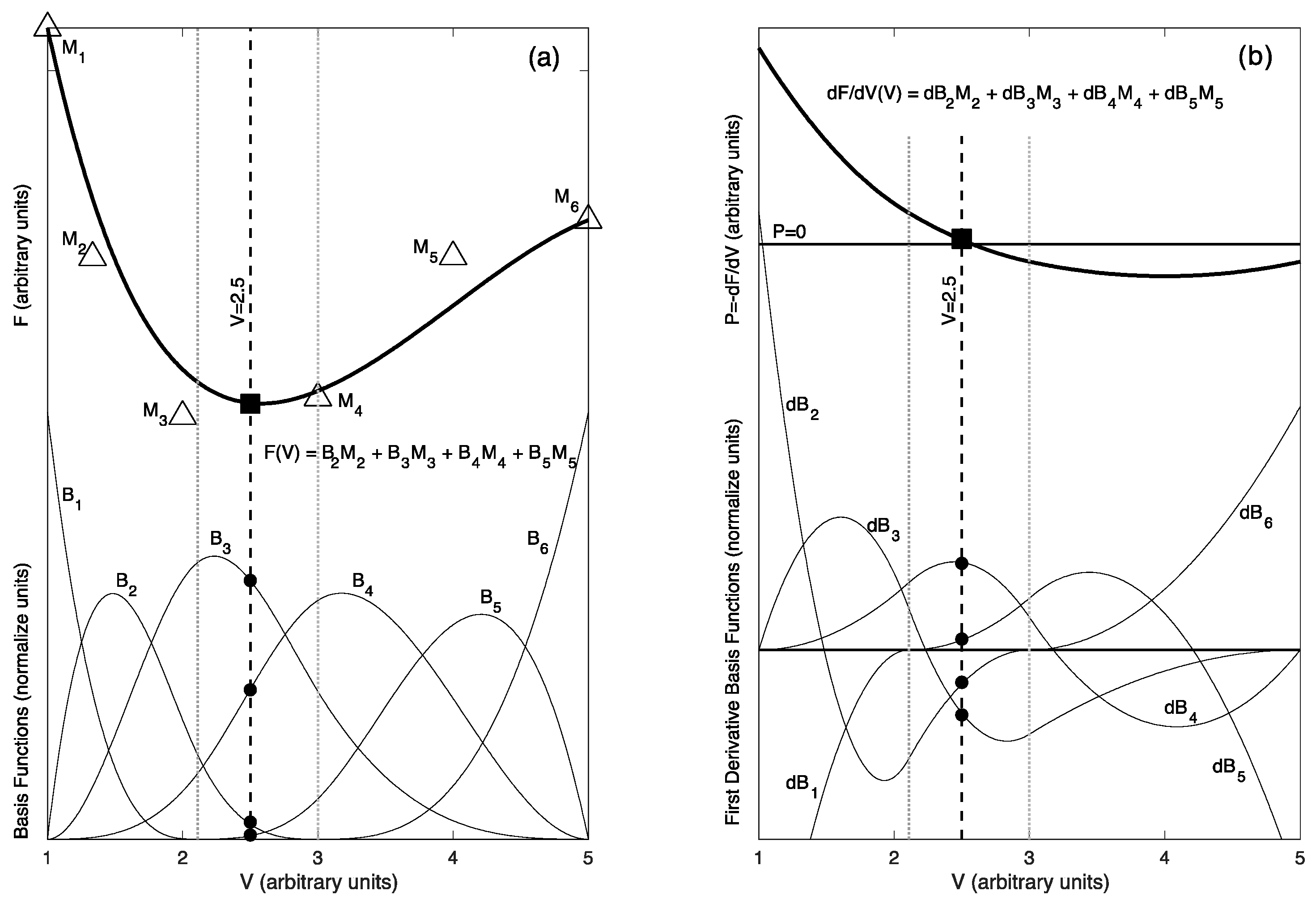
2.2. Local-Basis-Function Representation of Helmholtz Energy

Numerical methods, developed to meet modern computational speed and accuracy requirements as well as for computer-aided graphics applications, are shown in this section to provide an alternative framework for the representation of Helmholtz energy. Although standard quantities (e.g., trigonometric and logarithmic) can be determined numerically, interpolation of previously calculated values in lookup tables is more efficient. Various interpolation algorithms have been developed and are embedded in both modern hardware and software. Such methods can be applied to representation of Helmholtz energy since any empirically based equation of state is created as an accurate interpolating formula capable of matching all measurements and theory.

The linear interpolation of a list of energies at different volumes is the simplistic approach that can work with sufficiently dense tables. However, accurate smaller models are possible using better interpolating functions and mathematical forms can be chosen to aid construction of representations. Here, piece-wise polynomials on intervals (splines) are used to represent Helmholtz energy over wide ranges of compression. Within each interval, representations are numerically analogous to the conventional series expansion-based equations of state. However, having separate polynomials in different intervals gives greater flexibility in meeting the needs of the underlying physics.

In the following, b-splines [37] are used since they have a number of beneficial numerical properties that are further described below. A b-spline representation, in essence a lookup table, consists of two lists, one containing points defining intervals of the independent variable and a second containing the model parameters. Basis functions then provide the means to interpolate the table. A b-spline of order two (spline order is one greater than the degree of underlying polynomials) is equivalent to linear interpolation of model parameters as a function of the independent variable. In this case, the representation has discontinuous derivatives at interval boundaries. With increasing b-spline order (using higher degree polynomials within each interval) the number of continuous derivatives at interval boundaries increases. The size of a b-spline equation of state is larger than that of a conventional representation. In addition to coefficients required for any global polynomial representation, at least one additional model parameter is needed for each added interval. As shown later, only a few intervals are needed to achieve adequate representations and the model size remains small.

Key properties of b-spline basis functions that make their use advantageous for equation of state representations include:

• B-spline basis function values are available in all computer environments as a call to a function/subroutine. Analogous to the use of exponential or trigonometric functions, no custom (user) programing is necessary for use of b-spline basis functions. The evaluation of equation of state properties then uses universal calling functions that are not material specific.
• The calculation of values and derivatives of a b-spline model are based on linear programing. Interpolation using b-splines is essentially a weighted average of neighboring model parameters with the basis functions providing the normalized weights. This enables efficient computer algorithms for both construction and evaluation of spline models. Arbitrary precision is possible in representing any functional behavior.
• B-spline basis functions are localized. Unlike global polynomial fits of data, spline model parameters pertain to the behavior of the underlying function in a separate restricted regime of the independent variable.
• Details of how intervals are defined allow flexibility in the behavior of function derivatives at interval boundaries. It is possible to allow discontinuities of the function or specified derivatives of the function at a location to meet the needs of a particular equation of state that might involve higher-order transitions.

Additional b-spline details are important in understanding their use for equations of state representations. The full articulation of the underlying mathematics is provided by de Boor [29]. Only a short overview that emphasizes points relevant to the current applications is provided in Appendix A. These include further articulation of spline order, model parameters, and b-spline basis functions. Also included is a description of the interval boundaries, the knots, and how local derivatives are controlled by knot multiplicity. An example representation of Helmholtz energy is given to further illustrate the underlying concepts.

Although spline representations of data can be constructed using standard numerical packages, the concept of local-basis-function (LBF) equation of state representations, as developed here, emphasizes the use of physics-based constraints during their construction. This was introduced in Brown [38], where Gibbs energy was expanded as a function of pressure and temperature. An equation of state for water based on Gibbs energy LBF representations is given in Bollengier et al. [39] and for high pressure ices in Journaux et al. [40]. Here, Helmholtz energy, with volume as the independent variable, is the focus. The representations are extended far beyond the regime of measurement using theory-based constraints for limiting behavior (i.e., a constraint on the pressure derivative of the bulk modulus at infinite pressure based on the Thomas–Fermi electron gas limit).

2.3. Determination of Helmholtz Energy by Collocation

Helmholtz energy, a surface in volume and temperature, can be reconstructed through collocation. Collocation is a standard approach for the numerical solution of differential equations in which basis functions are chosen that match differential properties at specified points, the collocation points. In addition, integrating constants must be applied. Here, considering only the volume axis of energy at 300 K, measurements, theory, and physical insight constrain derivatives of the energy surface at specified collocation sites. A sufficiently flexible set of b-spline basis functions then allows representation of any plausible physical behavior for Helmholtz energy and its derivative properties. Here, the arbitrary energy “datum” is set to zero at equilibrium. The challenges lie in the details of data selection, articulation of what constitutes adequate fitting as opposed to overfitting of data, and how to constrain behavior in data-poor regimes.

Such challenges are not unique to equation of state studies and are described within the rubric of parameter estimation using inverse methods [41]. Here, the “damped least square method” or Tikhonov inversion is used to determine model parameters for equation of state representations. The minimization of one or more side constraints (hereafter called regularization) is added to the standard least square solution. A straightforward approach based on physical insight is to minimize a specified derivative of the model. A smooth model would be one with the smallest second derivatives while still adequately fitting data. In the case of equations of state represented by energy potentials, the second derivative of the Helmholtz energy figures into the determination of the bulk modulus (as shown in Equation (3)), a third derivative is needed to determine K’ and a fourth derivative is needed to determine K”. Since K’ is a frequent quantity of interpretation and since it is typically found to be smooth and trending to an asymptotic value at infinite pressure, minimizing the fourth derivative of the Helmholtz energy emerges as a possible side constraint. Linear inverse methods then allow determination of the model parameters, fitting pressure–volume (and/or bulk moduli) data with a side constraint on the derivative of energy. The explicit minimization of the third derivative of the bulk modulus (to make K’ smooth or to require a specific value for K’) is undertaken with non-linear analysis. Further details of inverse theory are described in Appendix A.

In summary, a framework is described to find Helmholtz energy by collocation of measurements, theory, and physical insight (through use of regularization) over arbitrarily large regimes of compression. Local-basis-functions (LBF) based on piece-wise polynomials in the form of b-splines are used. A linear problem allows fits of pressure–volume and bulk modulus–volume measurements. Fits involving determinations of the bulk modulus as a function of pressure and its pressure derivatives requires iterative and non-linear analysis. The resulting representations for Helmholtz energy have model parameters in units of energy that can be analytically evaluated for equation of state properties including pressure, the bulk modulus, and derivatives of bulk modulus as a function of volume (or density). The numerical function to evaluate properties based on the LBF representation is universal, no material-specific coding is required.

A number of decisions are required in the creation of an LBF representation for Helmholtz energy. An optimal choice of strain metric may reduce model size. The number of intervals for strain (as well as their distribution and bounds) can be varied. The cost of subdivision is that at least one additional model parameter is required for each added interval of representation. The total parameter count grows slowly since boundary conditions (matching values and derivatives of values at boundaries) reduce the required number of unique parameters. The order of a chosen basis function set is arbitrary and might depend on the physics of a specific material. Smaller intervals allow lower order fits. The derivative of the potential used for regularization is an arbitrary choice. Additional non-linear optimization is required if a specific limiting value for the pressure derivative of the bulk modulus is required.

Using the MATLAB numerical environment, a set of tools based on the concepts given here are provided with the Supplementary Materials. They allow creation and evaluation of LBF equations of state. Scripts using these tools are also provided that reproduce the analyses given in the following sections.

3. Results

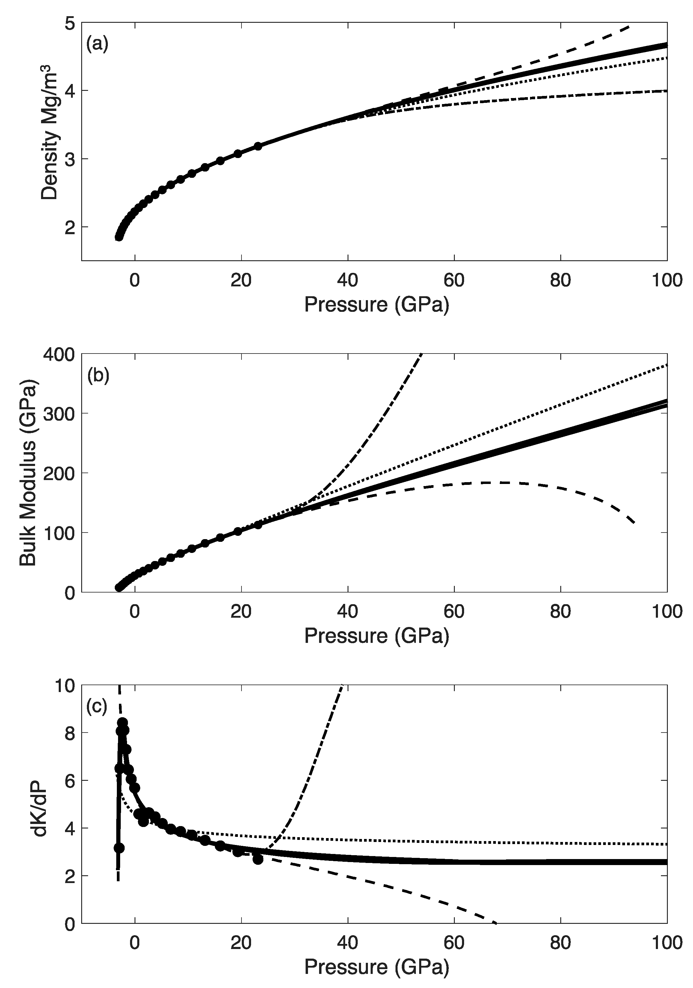
3.1. Equations of State for NaCl

3.1.1. Data and Representations

Measured volumes of NaCl provide an internal pressure calibrant in some high-pressure experiments [42]. The widely used pressure scale for NaCl given by Decker (1971) [43] was based on an assumed two-term pair-wise interaction energy potential. Accurate high-pressure data obtained subsequent to Decker’s work exhibited systematic deviations from his pressure scale. Brown (1999) [44] reported an energy potential for NaCl that provides a better representation of accurate high-pressure and high-temperature measurements. Here, properties on the zero Kelvin isotherm, tabulated in [44], provide precise quantities to evaluate the current method of representation. The data and an example script illustrating the analysis given in this section are provided in Supplementary Materials. The fitting is constrained by both pressure–volume and bulk modulus data. The relative weight of these data was adjusted to provide a satisfactory balance between simultaneous fits of pressures and the bulk moduli as a function of volume.

In Figure 1 the zero-Kelvin densities (panel a), bulk modulus (panel b), and its pressure derivative (panel c) as tabulated in [44] are plotted as a function of pressure. Lines show equation of state predictions based on the model parameters given in

Table 2. Equation of state parameters and root-mean-square (rms) misfits of pressure (P_rms) and the bulk modulus (K_rms) for representations of the NaCl 0 K isotherm. A 1 bar density of 2.226 Mg/m³ is used in all representations. Units for all parameters are shown.

Type of Function	Parameters				(rms)
Global-Basis-Function
Third order/degree Eulerian Finite Strain	Ko = 28.0 GPa	Ko’ = 4.5			Prms = 0.15 GPa Krms = 2.3 GPa
Fourth order/degree Eulerian Finite Strain	Ko = 27.4 GPa	Ko’ = 5.4		Ko” = −0.44 GPa−1	Prms = 0.02 GPa Krms = 0.3 GPa
Ninth order/degree Eulerian Finite Strain	Ko = 27.8 GPa	Ko’ = 5.4		Ko” = −0.67 GPa−1	Prms = 0.01 GPa Krms = 0.2 GPa
	(Five more parameters for the ninth order fit are not reported here. See Supplementary Materials)
Local-Basis-Function:
	Knots (strain units):		Coefficients (GPa m3/Mg)
Eulerian Finite Strain Order: 6 (degree 5)	[−0.08, −0.035, 0.24, 0.67] (first and last knots are repeated six times)		[0.308, 0.242, −0.155, −0.292, 4.10, 10.9, 19.8, 26.1]		Prms = 0.01 GPa Krms = 0.2 GPa
log Strain Order: 5 (degree 4)	[−0.09, −0.036, 0.2, 0.42] (first and last knots are repeated five times)		[0.326, 0.241, −0.141, −0.326 3.92 16.4 26.0]		Prms = 0.01 GPa Krms = 0.2 GPa

. Data misfits are listed in Table 2. Values extend from negative pressures (constrained by high-temperature measurements at 1 bar) to the high-pressure limit of the NaCl B1 structure.

Properties are plotted in Figure 1 to pressures beyond the stability regime of the B1 structure to examine the behavior of each equation of state in extrapolation. Both conventional global fits (Birch-Murnaghan third and fourth order) and a non-standard global fit (ninth-order), all based on Equation (2), are illustrated. Local-basis-function (LBF) representations (using both Eulerian and log strain metrics) are also shown.

3.1.2. Discussion

The energy potential for NaCl over the extended range of volume compression samples significantly different physical behavior. Expanded state properties (negative pressures) are more strongly influenced by long-range cohesive forces (including Coulomb and inductive). In the compressed state, the overlap of electrons creates large short-range repulsive interactions. The large variation of K’ values with a maximum just below ambient pressure provides evidence that the underlying potential is more complex than one that can be represented by a global low order series expansion.

In Figure 1 all equations of state in the regime of measurements provide adequate approximation to values and trends in density and the bulk modulus. Unsurprisingly, as shown in Table 2, misfit is largest for the third-order representation and this lower order fit has an unsatisfactory representation of the pressure dependence of K’. The fourth-order version, while providing a more plausible fit of measurements in the compressed regime, does not have sufficient flexibility to follow the behavior of K’ in the expanded state. The fourth-order predicted pressure derivative of the bulk modulus continues to increase as pressure becomes increasingly negative. The data show a maximum in K’ slightly below ambient pressure as required by the necessary behavior of the energy of interaction in the expanded state. As a result of a need for significant curvature of the bulk modulus as a function of pressure near equilibrium (requiring a large second derivative of the bulk modulus), the behavior of the bulk modulus for the global fourth-order fit at high pressure is unstable; K’ implausibly goes through zero to negative values and the bulk modulus decreases with increasing pressure. A ninth-order fit proved to be the lowest order global representation that could adequately represent all data. As expected, this equation of state cannot be extrapolated.

The LBF equations of state are constructed to have satisfying performance from the expanded state to high compression. They are required to adequately fit data while extrapolating with appropriate physics-based limiting behavior. Two versions (graphically indistinguishable) are shown that fit data equally well. One LBF uses Eulerian finite strains and the other uses log strains. The log strain version allowed use of a lower order spline (order 5) than the Eulerian strains did (order 6). Both LBFs use three intervals (two in the low-pressure regime, and one extending well beyond the regime of measurements). The high-pressure behavior for both was constrained by requiring that the fourth derivative of the potential be small and that the high-pressure limit of K’ be greater than 5/3 [45,46]. The high-pressure constraint on K’ was enforced through non-linear optimization of an initial linear model. In this case, it is a choice to slightly misfit the pressure derivative of the bulk modulus for the highest-pressure data as a necessary consequence of enforcing the smooth asymptotic behavior for K’. Here, physical insight is given more weight that the accuracy of a single data point at the extreme of the measurements.

The key findings of this section include the following: (1) Standard forms for equations of state based on global representations using series expansions of the Helmholtz energy can neither capture the details of NaCl behavior in regimes of measurement nor do they correctly extrapolate to high pressure. (2) Higher order global fits can be constructed that adequately fit all data, but even modest extrapolation is impossible. (3) In contrast, an LBF representation having three volume intervals (one extending well beyond measurements) can both better represent data and provides plausible (physics-based) behavior well beyond any possible measurement. (4) The choice of strain metric has no impact on the quality of the fit. (5) The behavior of representations in regions of extrapolation can be adjusted to match theory-based constraints. (6) The model size of the LBF representations are larger (a dozen or so parameters) compared to three for a global fourth-order fit. However, this is not a serious impediment to their use.

3.2. Equations of State for High Pressure Ice (Ice VII–X System)

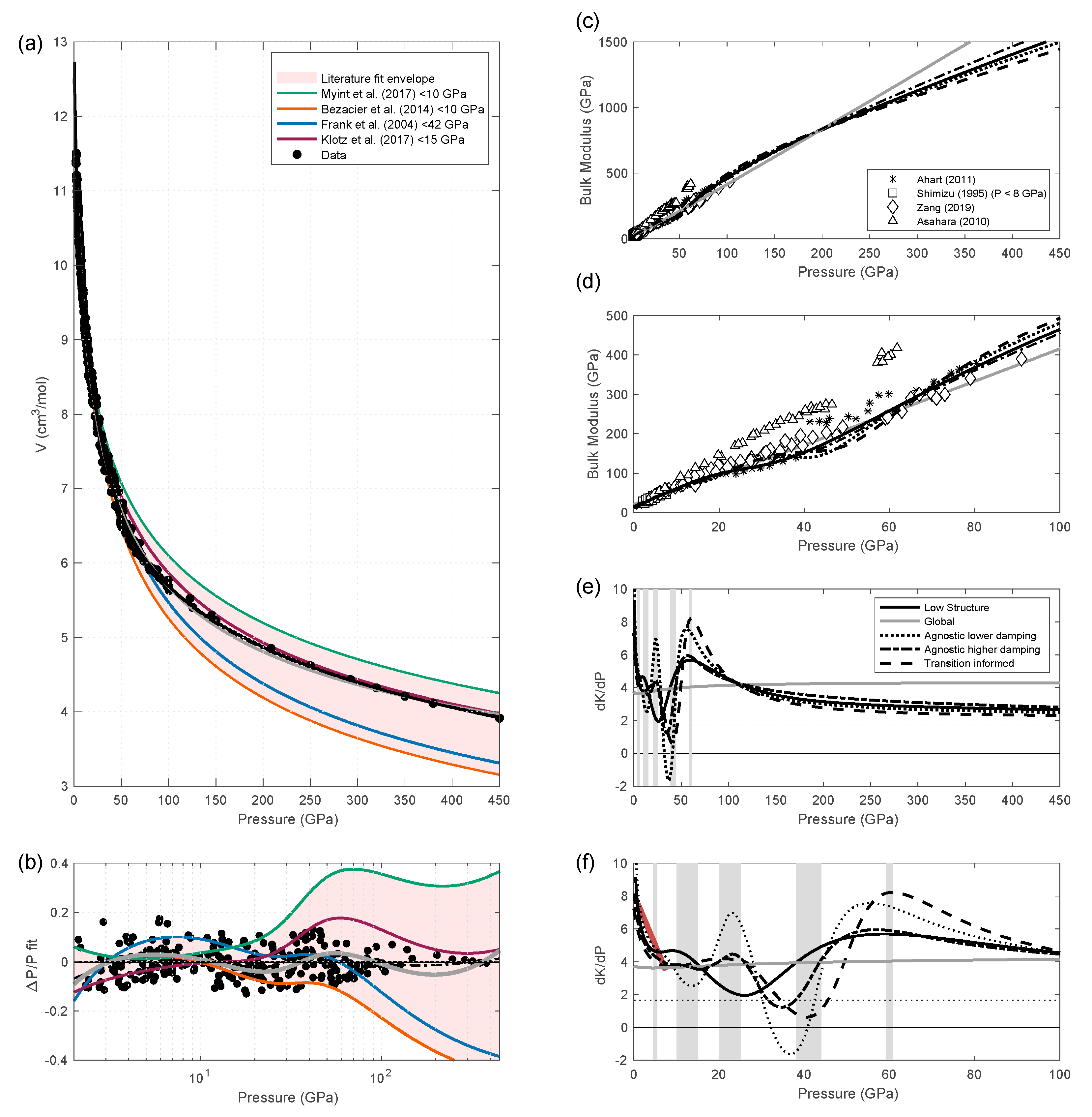
3.2.1. Data and Representations

Based on the success of local-basis-function representations in the previous section, attention is focused on the ice VII–ice X system to 450 GPa. The upper pressure limit of this representation is associated with the span of the density-functional (DFT) calculations. Equations of state at 300 K are constructed minimizing the root-mean-square (rms) misfit to 291 selected pressure–volume points from 16 independent datasets. While independently determined values for the bulk modulus have been reported and are discussed below, these data were not directly used as fitting constraints. Data and the numerical analysis are provided as scripts with the Supplementary Materials. Both experimental [15,16,17,21,33,47,48,49,50,51,52,53,54,55,56,57] and DFT studies [51,52] are considered. Results above 150 GPa are based solely on theory. The results in [15], that used an experimental method for pressure calibration, and measurements reported in [16], that deviate substantially from other work, are excluded in the current fits. Inclusion of these data increases the root-mean-square (rms) misfit but does not change the interpretations given below. No additional quality-of-data assessment is undertaken in the current analysis. Biases associated with systematic and random errors are likely reduced in the current meta-analysis of all data. The sample size may be sufficient to diminish the impact of small disagreements between merged datasets, arising from the use of different pressure gauges, volume measurement techniques, or experimental protocols that may affect biases associated with non-hydrostatic stresses. Pressure–volume data are plotted and compared with published equations of states [47,49,53,58] in Figure 2a.

To adequately explore the information contained in the pressure–volume measurements, an ensemble of representations was created based on differing assumptions for parameterizations and regularization. Examples are plotted in all panels of Figure 2, and parameters for these fits and associated misfits are listed in

Table 3. Equation of state parameters and root-mean-square (rms) pressure misfits (P_rms) for representations of high-pressure ice VII and X 300 K isotherm. Units for all parameters are shown. V_o for ice VII is taken from Klotz (2017): 12.7218 cm³/mol or 42.25 ų at 300 K.

Type of function	Parameters		(rms)
Global-Basis-Function
Fourth order/degree Eulerian Finite Strain	Ko = 19.2 GPa, Ko’ = 3.8, Ko” = −0.09 GPa−1		Prms = 3.0 GPa
Local-Basis-Function:
	knots (dimensionless strain):	Coefficients (GPa cm3/mole)
“Agnostic” log Strain low damping Order: 6 (degree 5)	[−0.01, 0.02, 0.04, 0.06, 0.08, 0.10, 0.12, 0.15, 0.17, 0.20, 0.24, 0.27, 0.31, 0.36, 0.42] (first and last knots are repeated six times)	[−0.10, −0.07, 0.05, 0.40, 1.37, 3.75, 7.13, 12.5, 20.0, 30.7, 46.7, 72.5, 103, 157, 254, 379, 520, 647, 723]	Prms = 1.7 GPa
“Agnostic” log Strain higher damping Order: 6 (degree 5)	[−0.01, 0.02, 0.04, 0.06, 0.08, 0.10, 0.12, 0.15, 0.17, 0.20, 0.24, 0.27, 0.31, 0.36, 0.42] (first and last knots are repeated six times)	[0.02, −0.03, −0.03, 0.23, 1.16, 3.55, 6.96, 12.3, 19.7, 30.4, 46.9, 71.5, 103, 157, 253, 375, 516, 645, 724]	Prms = 2.0 GPa
“low structure” log Strain (seven intervals) Order: 7 (degree 6)	[−0.01, 0.08, 0.12, 0.16, 0.16, 0.24, 0.3, 0.42] (first and last knots are repeated seven times)	[−0.09, −0.04, 0.43, 2.21, 6.50, 17.5, 46.3, 93.1, 153, 258, 433, 595, 723]	Prms = 2.0 GPa
“transition informed” log Strain (seven intervals) Order: 7 (degree 6)	[−0.01, 0.12, 0.16, 0.16, 0.21, 0.23, 0.26, 0.42] (first and last knots are repeated seven times)	[0.10, −0.27, 0.26, 2.86, 10.6, 25.6, 57.3, 104, 153, 263, 396, 556, 722]	Prms = 1.7 GPa

. The global fourth-order Eulerian representation, Equation (2), has the largest rms misfit. The LBF versions have reduced rms misfits. Although reduced misfit is expected for models containing more parameters, the global representation has greater systematic misfit and, as shown below, the LBF representations give results that better align with the lowest pressure bulk moduli data and the known complex phase behavior in the ice VII–X system. The LBF representation labeled “low structure” resulted from exploration (based on manual variation of knot placements) in which the goal was to find the smallest number of intervals with the least structure (smallest variations of K’). The impact of discontinuities in higher order derivatives of Helmholtz energy were tested by introducing knot multiplicity at boundaries that are manually aligned to match pressures for proposed higher-order phase transitions. One such fit labeled “transition informed” is reported and is further discussed below. “Agnostic” LBF fits were constructed using a sixth-order spline over 14 internal intervals to allow more than necessary flexibility in representing the equation of state with no preconceptions of where higher-order phase transitions might occur. Two examples demonstrate differing levels of regularization. Additional LBF representations, created to explore hypothesized pressure dependences of the bulk modulus, are discussed and rejected in the following discussion. Regularization, based on minimizing the fourth derivative of Helmholtz energy, was applied to the LBF models. The damping parameter for regularization was varied to find an optimal trade-off between misfit and model smoothness. The tradeoff is illustrated in Figure 3 where the rms average of the Helmholtz energy fourth derivative is plotted against rms misfit of the pressure–volume data. An infinite number of solutions are possible as the damping parameter is continuously changed. As shown in the figure, larger rms values for the fourth derivative allow smaller misfit at the cost of possibly over fitting data. As greater smoothing is enforced (larger damping), misfit increases, eventually becoming unacceptably large. Three points marked on the diagram are associated with the three levels of misfit reported in Table 3. Acceptable solutions for damped solutions are typically chosen near the corner of the trade-off curve, representing a compromise between data misfit and the degree of smoothness.

Fractional deviations from the “low-structure” representation of the pressure volume data and selected literature equations of state are plotted as a function of the logarithm of pressure in Figure 2b. As shown in this panel, the fractional deviations are relatively uniform as a function of pressure with a standard deviation near 5%. The highest-pressure points based on theory have greater precision with unknown accuracy but appear to merge into the more scattered measurements with little apparent offset or change in slope.

In Figure 2c (full pressure range) and d (lower pressure regime), predictions of the isothermal bulk modulus based the current equation of state are compared to reported adiabatic bulk modulus based on Brillouin acoustic measurements [31,59,60,61]. The difference between adiabatic and isothermal moduli is small in the high-pressure regime and is currently ignored. Although the conversion from sound speeds to elastic moduli requires knowledge of the density, the differences in density between the current representation and those used in the original studies had negligible impact at the scale of these figures. The measurements to 8 GPa reported by Shimizu et al. [60] for single crystals grown in equilibrium with liquid water provide plausible determinations of the bulk modulus. Other studies relied on longitudinal and transverse wave measurements in polycrystalline material with unknown fabric in a non-hydrostatic environment. In spite of the cubic symmetry for the high-pressure ices, such data may suffer from systematic biases.

Pressure derivatives of the bulk modulus based on our representations are shown in Figure 2e (full pressure range) and f (lower pressure regime). Also shown between 2 GPa and 8 GPa is the behavior of K’ as constrained by a quadratic fit to the single crystal measurements of Shimizu et al. Vertical bands in these panels indicate the pressure ranges for the suggested higher-order transitions listed in Table 1.

3.2.2. Discussion

The following discussion progresses through considerations of (1) the pressure–volume data, (2) the elastic bulk moduli determinations, and finally, (3) how variations of the pressure derivative of the bulk modulus correlate to pressure ranges where higher-order transitions likely occur. In the absence of transitions and as previously documented in Figure 1 for NaCl, values for the pressure derivative of the bulk modulus, K’, can range from more than 6 at low pressure to less than 3 at the highest pressures. The second derivative, K”, is usually small and negative. Possible changes of ice’s compressive behavior related to higher order transition as summarized in Table 1 include the following ideas. A possible distortion in the bcc lattice around 15 GPa is suspected to be the expression of the locking of OH-rotational disorder which could change the rate of stiffening under compression [51]. Changing derivatives of the bulk modulus near 25 GPa might reflect the transition from ice VII to ice VII’ associated with the start of dynamic translational proton disorder by tunneling and thermal hoping. The onset of the hydrogen bond symmetrization, with the transition towards H-translational disorder [51], should have an effect on compression beyond 40 GPa. Furthermore, a broad minimum in K’ would be the expected behavior for a second order transition between ice VII and a slightly higher density ice X phase.

In prior analyses of individual datasets, equations of state were constrained by data spanning restricted ranges of pressures. The envelopes of such regional fits, extrapolated to cover the entire range of pressure, are illustrated in Figure 2a,b. The various fits are essentially indistinguishable below 50 GPa (Figure 2a). Even at the scale of the residuals (Figure 2b), data scatter is as large as the envelop bounds. Unsurprisingly, predictions in regimes of extrapolation diverge and do not accurately match the highest-pressure DFT results.

The adequacy of representations as measured by the rms misfit to data is not immediately obvious in examination of just the pressure–volume relationships shown in Figure 2a,b. However, the trade-off curve shown in Figure 3 indicates that an rms misfit near 2 GPa is optimal. On this basis, the global fourth-order representation clearly underfits the data, while the low damping agnostic fit and the transition informed fit may overfit the data (as further discussed below).

Greater discrimination between equation of state representations is expected at the level of the derivative properties: the bulk modulus and its pressure derivative (all panels on the right side of Figure 2). For pressures below 8 GPa, K and K’ values determined from sound speed measurements are replicated in the LBF fits, indicating that the underlying pressure–volume data are sufficiently accurate and that the analysis can extract higher order derivatives of Helmholtz energy. In contrast, all global fits, both from prior literature and the current fourth-order, do not match the low-pressure behavior for K’. In order to approximate the volume trends over the entire range of pressures, all global fits require a nearly constant and low (~4) value for K’ since such global representations have insufficient flexibility to accommodate both behavior at low pressure and at high pressure. This mirrors the findings in the previous section with the effort to represent the NaCl equation of state. At the highest pressures, where only theory provides constraints, the LBF representations smoothly approach the Thomas–Fermi limit. No global representation provides correct limiting behavior. Furthermore, the current fourth-order global representation shows unphysical behavior with K’ increasing from 3.8 near zero pressure to a nearly constant value of approximately 4 at the highest pressure.

In the critical range of higher-order transitions for ice between 15 GPa and 60 GPa, the measured bulk moduli show disagreement between the independent studies and the LBF representations Whether these differences are caused by systematic errors in measurement, differences in non-hydrostatic stresses, or are indicative of material properties that vary with the time-scale of measurement, remains unresolved. A hypothetical relaxation time for a phase transition or for proton mobility that is large compared to the sub-nanosecond periods of acoustic wave measured in Brillouin experiments could rationalize the observation that the static moduli are smaller than the moduli based on sound speeds. Equation of state fits required to match the Brillouin-based bulk moduli in this pressure regime were found to systematically misfit the pressure–volume data. In contrast, the bulk moduli beyond 60 GPa [59,61] converge to a common pressure dependence that is consistent with predictions based on the LBF fits.

Focusing on K’ in Figure 2e,f, trends for its pressure dependence separate into three zones. In the low-pressure regime K’ decreases from a value near 6.5 at 2.2 GPa (similar to values for ice V and ice VI [40]) to about 4 for pressures between 10 to 15 GPa. As shown in the figure, this normal trend is in agreement with the Shimizu et al. determinations to 8 GPa. Above 60–70 GPa, K’ also shows normal behavior, an asymptotic decrease with pressure. In contrast, the intermediate pressure range, the previously identified regime of higher-order transitions, shows the most anomalous behavior for K’. All LBF representations show a minimum between 30 GPa and 40 GPa. The “agnostic” fits have shoulder maxima on the sides of the minimum values. One “agnostic” fit has an optimal misfit of 2 GPa (based on Figure 3). The other “agnostic” fit, with smaller rms misfit (that appears on the overfitting side of the trade-off curve), predicts that K’ dips below zero resulting in a local minimum of K as shown in Figure 2d. The “low structure” representation has a shallower minimum and no shoulder maxima around 25 GPa for the same (optimal) 2 GPa misfit. Since K’ is negative in the transition region only for the least damped “agnostic” solution, the bulk modulus does not generally “soften” (decrease at higher pressure). Instead, it simply fails to increase normally with pressure. The “transition informed” fit, created to better align features of K’ with identified pressures of transitions, has interval boundaries near the transition from dominant rotational disorder to more translational disorder around 15 GPa and the start of hydrogen symmetrization with the increase of translational disorder above 40 GPa, with a full transition to ice X above 60–80. As shown in Table 3, the misfit for the “transition informed” representation is reduced at the cost of a higher rms average for the fourth derivative of Helmholtz energy. Whether this represents over fitting data remains to be determined.

The key findings of this section reinforce those associated with the effort to represent NaCl. Conventional equation of state global representations can provide approximations to all pressure–volume data at the expense of predicted bulk moduli that are not in accord with low pressure measurements and exhibit incorrect high-pressure limiting behavior. Local-basis-function representation for high-pressure ice are able to better satisfy these strong side constraints. However, for the ice VII–X continuum, in the regime of higher-order phase transitions, an infinite number of representations are possible that fit the data within plausible bounds. The ensemble reported here provide examples of trade-off possibilities between misfit to data and allowable structure of the fits. Representations can have features of K’ aligned with expected transitions on the basis of a priori constraints although such close alignment is not required by the pressure–volume data alone. The most robust features of all members of successful fits are a decrease in K’ from normal values near 15 GPa to a minimum in the 25 to 40 GPa range followed by an increase to 60–70 GPa followed by normal asymptotic decreases at much higher pressures. No fit required to follow measured bulk moduli in the 25 to 60 GPa range provided an adequate representation of the pressure–volume data. Whether this is a result of errors in data or is an indication of a rate-dependent process remains undetermined.

4. Discussion

A representation of Helmholtz energy at 300 K for ice VII–X was developed in order to better understand the complexity of high-pressure ices that exist as mineral phases in this solar system and beyond. Questions of origins and evolution require knowledge of an underlying equation of state. The results of this investigation are summarized in the concluding section. In order to accomplish the principal goal, coverage of a broad set of concepts and analysis was necessary. Topics include a foundational review about the nature of numerical representations for equations of state, an exposition describing a new framework for representations, and articulation of important details associated with the new framework. Both interpolation and inverse problems are widely recognized challenges in data assimilation. Methods, previously found useful in other fields, are adapted and modified to meet the unique requirements of Helmholtz energy representations.

The underlying premise is that equations of state must provide coherent empirical representations of all measurement-constrained and theory-based knowledge of a material. The previous generation of parameterizations under performed in this task as a result of a bias towards using physics-blind models with insufficient flexibility. This lack of flexibility resulted in discussions that shifted to numerical issues such as “What constitutes the best strain metric?” and “Which order expansion is preferred?”. The current analysis refocuses attention. The behavior of an equation of state should be physics-based and basis-function independent. The total number of model parameters required is less important than how well the representation matches the constraining information. Finding the best representation involves determining the appropriate relative weighting of data from varied sources, assessing the quality of results based on theory, and applying suitable side-constraints based on the best physical insight. Decisions based on these ideas were specifically expressed during the construction of equations of state for NaCl and high-pressure ice.

The new equation of state analysis is a seminal step beyond the earlier generation of Helmholtz energy-based parameterizations that use polynomial series expansions of an arbitrarily defined strain metric. Here, a single global polynomial is replaced with flexible local piece-wise polynomials in the form of b-splines. The new local-basis-function representations are more than simple spline fits of data since their creation is embedded in an inverse theory framework of parameter estimation by Tikhonov inversion that requires incorporation of physics-based constraints and insight. An important characteristic of inverse theory solutions is the ability to explore features shared by all possible representations of data. A key strength of this approach, demonstrated in the effort to represent ice, is the power to ask both what model features are required by data and conversely what are data requirements to adequately delineate model features.

5. Conclusions

A large body of measurements and theory for ice VII–X were assimilated into an equation of state covering pressures up to 450 GPa. Selected pressure–volume data from 14 experimental studies and two theoretical reports were then accurately represented. In addition, separately measured derivative properties (the bulk modulus and its pressure derivative) were replicated both in low-pressure and high-pressure regimes, indicating that the underlying pressure–volume data are sufficiently accurate and that the current analysis can extract higher order derivatives. Anomalies in the bulk modulus (and its derivative) were found to roughly align with proposed higher-order transitions at intermediate pressures. However, in this range, bulk moduli determined using GHz-frequency Brillouin experiments did not match the static determination. The differences between results from different groups leaves open the possibility that systematic experimental errors remain large. Alternatively, a relaxation time-constant for the underlying high-order phase transition or for proton mobility may be large compared to the frequencies used in acoustic measurements. The pressure–volume data can resolve variations of the second derivative of the bulk modulus with pressure. However, discontinuities in K” and/or the precise locations of features in the pressure derivative of the bulk modulus are not currently resolvable. Improved high-pressure determinations of derivative properties could provide better constraints for the next-generation representations. More generally, the tools and methodologies developed here can be broadly applied in other high-pressure equation of state studies.

Articulation of the necessary background for b-splines and for parameter estimation is placed in Appendix A. A small toolbox containing five functions and example scripts written in the MATLAB numerical environment are also provided with the Supplementary Materials. MATLAB is convenient for exploration of the ideas presented in this paper. The open source environment OCTAVE is compatible with the provided MATLAB functions and scripts and can be downloaded for no cost. PYTHON and FORTRAN implementations can easily be created.

In the provided MATLAB scripts, the analysis requires four steps: (1) load data, (2) set options, (3) fit data, (4) display results. This provides a straightforward workflow that encourages exploration of how modifications of assumptions provide differences in the resulting equation of state. It is important to try modifications of all adjustable elements in order to explore the parameter sensitivity and quality variations of fits.

References

1. Tschauner, O.; Huang, S.; Greenberg, E.; Prakapenka, V.B.; Ma, C.; Rossman, G.R.; Shen, A.H.; Zhang, D.; Newville, M.; Lanzirotti, A.; et al. Ice-VII inclusions in diamonds: Evidence for aqueous fluid in Earth’s deep mantle. Science 2018, 359, 1136–1139. [Google Scholar] [CrossRef] [Green Version]
2. Léger, A.; Selsis, F.; Sotin, C.; Guillot, T.; Despois, D.; Mawet, D.; Ollivier, M.; Labèque, A.; Valette, C.; Brachet, F. A new family of planets? Icarus 2004, 169, 499–504. [Google Scholar] [CrossRef] [Green Version]
3. Sotin, C.; Grasset, O. Mass-radius curve for extrasolar Earth-like planets and ocean planets. Icarus 2007, 191, 337–351. [Google Scholar] [CrossRef]
4. Noack, L.; Höning, D.; Rivoldini, A.; Heistracher, C.; Zimov, N.; Journaux, B.; Lammer, H.; Van Hoolst, T.; Bredehöft, J.H. Water-rich planets: How habitable is a water layer deeper than on Earth? Icarus 2016, 277, 215–236. [Google Scholar] [CrossRef]
5. Vance, S.D.; Panning, M.P.; Stähler, S.; Cammarano, F.; Bills, B.G.; Tobie, G.; Kamata, S.; Kedar, S.; Sotin, C.; Pike, W.T.; et al. Geophysical investigations of habitability in ice-covered ocean worlds: Geophysical habitability. J. Geophys. Res. Planets 2018, 123, 180–205. [Google Scholar] [CrossRef] [Green Version]
6. Journaux, B.; Daniel, I.; Petitgirard, S.; Cardon, H.; Perrillat, J.-P.; Caracas, R.; Mezouar, M. Salt partitioning between water and high-pressure ices. Implication for the dynamics and habitability of icy moons and water-rich planetary bodies. Earth Planet. Sci. Lett. 2017, 463, 36–47. [Google Scholar] [CrossRef]
7. Unterborn, C.T.; Desch, S.J.; Hinkel, N.R.; Lorenzo, A. Inward migration of the TRAPPIST-1 planets as inferred from their water-rich compositions. Nat. Astron. 2018, 2, 297–302. [Google Scholar] [CrossRef] [Green Version]
8. Kite, E.S.; Ford, E.B. Habitability of exoplanet waterworlds. arXiv 2018, arXiv:1801.00748 [astro-ph]. [Google Scholar] [CrossRef] [Green Version]
9. Hendrix, A.R.; Hurford, T.A.; Barge, L.M.; Bland, M.T.; Bowman, J.S.; Brinckerhoff, W.; Buratti, B.J.; Cable, M.L.; Castillo-Rogez, J.; Collins, G.C.; et al. The NASA Roadmap to Ocean Worlds. Astrobiology 2019, 19, 1–27. [Google Scholar] [CrossRef] [Green Version]
10. Birch, F. Elasticity and constitution of the Earth’s interior. J. Geophys. Res. 1952, 57, 227–286. [Google Scholar] [CrossRef]
11. Stacey, F.D.; Brennan, B.J.; Irvine, R.D. Finite strain theories and comparisons with seismological data. Geophys. Surv. 1981, 4, 189–232. [Google Scholar] [CrossRef]
12. Benoit, M.; Bernasconi, M.; Focher, P.; Parrinello, M. New High-Pressure Phase of Ice. Phys. Rev. Lett. 1996, 76, 2934–2936. [Google Scholar] [CrossRef] [PubMed]
13. Hermann, A.; Ashcroft, N.W.; Hoffmann, R. High pressure ices. Proc. Natl. Acad. Sci. USA 2012, 109, 745–750. [Google Scholar] [CrossRef] [Green Version]
14. Millot, M.; Coppari, F.; Rygg, J.R.; Correa Barrios, A.; Hamel, S.; Swift, D.C.; Eggert, J.H. Nanosecond X-ray diffraction of shock-compressed superionic water ice. Nature 2019, 569, 251–255. [Google Scholar] [CrossRef] [PubMed]
15. Hemley, R.J.; Jephcoat, A.P.; Mao, H.K.; Zha, C.S.; Finger, L.W.; Cox, D.E. Static compression of H2O-ice to 128 GPa (1.28 Mbar). Nature 1987, 330, 737–740. [Google Scholar] [CrossRef]
16. Loubeyre, P.; Letoullec, R.; Wolanin, E.; Hanfland, M.; Häusermann, D. Modulated phases and proton centering in ice observed by X-ray diffraction up to 170 GPa. Nature 1999, 397, 503–506. [Google Scholar] [CrossRef]
17. Sugimura, E.; Iitaka, T.; Hirose, K.; Kawamura, K.; Sata, N.; Ohishi, Y. Compression of H2O ice to 126 GPa and implications for hydrogen-bond symmetrization: Synchrotron x-ray diffraction measurements and density-functional calculations. Phys. Rev. B 2008, 77, 214103. [Google Scholar] [CrossRef]
18. Goncharov, A.F.; Struzhkin, V.V.; Somayazulu, M.S.; Hemley, R.J.; Mao, H.K. Compression of Ice to 210 Gigapascals: Infrared Evidence for a Symmetric Hydrogen-Bonded Phase. Science 1996, 273, 218–220. [Google Scholar] [CrossRef]
19. Zha, C.-S.; Hemley, R.J.; Gramsch, S.A.; Mao, H.; Bassett, W.A. Optical study of H2O ice to 120GPa: Dielectric function, molecular polarizability, and equation of state. J. Chem. Phys. 2007, 126, 074506. [Google Scholar] [CrossRef]
20. Meier, T.; Petitgirard, S.; Khandarkhaeva, S.; Dubrovinsky, L. Observation of nuclear quantum effects and hydrogen bond symmetrisation in high pressure ice. Nat. Commun. 2018, 9, 1–7. [Google Scholar] [CrossRef] [Green Version]
21. Grande, Z.M.; Huang, C.; Smith, D.; Smith, J.S.; Boisvert, J.H.; Tschauner, O.; Steffen, J.H.; Salamat, A. Bond strengthening in dense H2O and implications to planetary composition. arXiv 2019, arXiv:1906.11990 [astro-ph, physics:cond-mat]. [Google Scholar]
22. Hirai, H.; Kadobayashi, H.; Matsuoka, T.; Ohishi, Y.; Yamamoto, Y. High pressure X-ray diffraction and Raman spectroscopic studies of the phase change of D2O ice VII at approximately 11 GPa. Int. J. High Press. Res. 2014, 34, 289–296. [Google Scholar] [CrossRef]
23. Somayazulu, M.; Shu, J.; Zha, C. In situ high-pressure x-ray diffraction study of H2O ice VII. J. Chem. Phys. 2008, 128, 064510. [Google Scholar] [CrossRef] [PubMed]
24. Pruzan, P.; Chervin, J.-C.; Gauthier, M. Raman Spectroscopy Investigation of Ice VII and Deuterated Ice VII to 40 GPa. Disorder in Ice VII. Europhys. Lett. 1990, 13, 81–87. [Google Scholar] [CrossRef]
25. Zha, C.-S.; Tse, J.S.; Bassett, W.A. New Raman measurements for H2O ice VII in the range of 300 cm−1 to 4000 cm−1 at pressures up to 120 GPa. J. Chem. Phys. 2016, 145, 124315. [Google Scholar] [CrossRef] [Green Version]
26. Guthrie, M.; Boehler, R.; Tulk, C.A.; Molaison, J.J.; dos Santos, A.M.; Li, K.; Hemley, R.J. Neutron diffraction observations of interstitial protons in dense ice. Proc. Natl. Acad. Sci. USA 2013, 110, 10552–10556. [Google Scholar] [CrossRef] [Green Version]
27. Yoshimura, Y.; Stewart, S.T.; Somayazulu, M.; Mao, H.; Hemley, R.J. High-pressure x-ray diffraction and Raman spectroscopy of ice VIII. J. Chem. Phys. 2006, 124, 024502. [Google Scholar] [CrossRef]
28. Okada, T.; Iitaka, T.; Yagi, T.; Aoki, K. Electrical conductivity of ice VII. Sci. Rep. 2014, 4, 5778. [Google Scholar] [CrossRef] [Green Version]
29. Noguchi, N.; Okuchi, T. Self-diffusion of protons in H2O ice VII at high pressures: Anomaly around 10 GPa. J. Chem. Phys. 2016, 144, 234503. [Google Scholar] [CrossRef]
30. Polian, A.; Grimsditch, M. New High-Pressure Phase of H2O: Ice X. Phys. Rev. Lett. 1984, 52, 1312–1314. [Google Scholar] [CrossRef]
31. Asahara, Y.; Hirose, K.; Ohishi, Y.; Hirao, N.; Murakami, M. Thermoelastic properties of ice VII and its high-pressure polymorphs: Implications for dynamics of cold slab subduction in the lower mantle. Earth Planet. Sci. Lett. 2010, 299, 474–482. [Google Scholar] [CrossRef]
32. French, M.; Redmer, R. Construction of a thermodynamic potential for the water ices VII and X. Phys. Rev. B 2015, 91, 014308. [Google Scholar] [CrossRef] [Green Version]
33. Wolanin, E.; Pruzan, P.; Chervin, J.; Canny, B.; Gauthier, M.; Häusermann, D.; Hanfland, M. Equation of state of ice VII up to 106 GPa. Phys. Rev. B 1997, 56, 5781–5785. [Google Scholar] [CrossRef]
34. Davies, G.F. Quasi-harmonic finite strain equations of state of solids. J. Phys. Chem. Solids 1973, 34, 1417–1429. [Google Scholar] [CrossRef]
35. Poirier, J.-P.; Tarantola, A. A logarithmic equation of state. Phys. Earth Planet. Inter. 1998, 109, 1–8. [Google Scholar] [CrossRef]
36. Vinet, P.; Rose, J.H.; Ferrante, J.; Smith, J.R. Universal features of the equation of state of solids. J. Phys. Condens. Matter 1989, 1, 1941. [Google Scholar] [CrossRef]
37. de Boor, C. A Practical Guide to Splines, Rev. ed.; Springer: New York, NY, USA, 2001; ISBN 978-0-387-95366-3. [Google Scholar]
38. Brown, J.M. Local basis function representations of thermodynamic surfaces: Water at high pressure and temperature as an example. Fluid Phase Equilibria 2018, 463, 18–31. [Google Scholar] [CrossRef]
39. Bollengier, O.; Brown, J.M.; Shaw, G.H. Thermodynamics of pure liquid water: Sound speed measurements to 700 MPa down to the freezing point, and an equation of state to 2300 MPa from 240 to 500 K. J. Chem. Phys. 2019, 151, 054501. [Google Scholar] [CrossRef]
40. Journaux, B.; Brown, J.M.; Pakhomova, A.; Collings, I.E.; Petitgirard, S.; Espinoza, P.; Ballaran, T.B.; Vance, S.D.; Ott, J.; Cova, F.; et al. Holistic Approach for Studying Planetary Hydrospheres: Gibbs Representation of Ices Thermodynamics, Elasticity, and the Water Phase Diagram to 2300 MPa. J. Geophys. Res. Planets 2020, 125, e2019JE006176. [Google Scholar] [CrossRef]
41. Aster, R.C.; Borchers, B.; Thurber, C.H. Parameter Estimation and Inverse Problems, Waltham; Academic Press: Cambridge, MA, USA, 2012. [Google Scholar]
42. Strässle, T.; Klotz, S.; Kunc, K.; Pomjakushin, V.; White, J.S. Equation of state of lead from high-pressure neutron diffraction up to 8.9 GPa and its implication for the NaCl pressure scale. Phys. Rev. B 2014, 90, 014101. [Google Scholar] [CrossRef] [Green Version]
43. Decker, D.L. High-pressure equation of state for NaCl, KCl, and CsCl. J. Appl. Phys. 1971, 42, 3239–3244. [Google Scholar] [CrossRef] [Green Version]
44. Brown, J.M. The NaCl pressure standard. J. Appl. Phys. 1999, 86, 5801–5808. [Google Scholar] [CrossRef]
45. Stacey, F.D.; Davis, P.M. High pressure equations of state with applications to the lower mantle and core. Phys. Earth Planet. Inter. 2004, 142, 137–184. [Google Scholar] [CrossRef]
46. Stacey, F.D. The K-primed approach to high-pressure equations of state. Geophys. J. Int. 2000, 143, 621–628. [Google Scholar] [CrossRef] [Green Version]
47. Bezacier, L.; Journaux, B.; Perrillat, J.-P.; Cardon, H.; Hanfland, M.; Daniel, I. Equations of state of ice VI and ice VII at high pressure and high temperature. J. Chem. Phys. 2014, 141, 104505. [Google Scholar] [CrossRef] [PubMed]
48. Bridgman, P.W. Freezings and Compressions to 50,000 kg/cm2. J. Chem. Phys. 1941, 9, 794–797. [Google Scholar] [CrossRef]
49. Fei, Y.; Mao, H.; Hemley, R.J. Thermal expansivity, bulk modulus, and melting curve of H2O–ice VII to 20 GPa. J. Chem. Phys. 1993, 99, 5369–5373. [Google Scholar] [CrossRef]
50. Frank, M.; Fei, Y.; Hu, J. Constraining the equation of state of fluid H2O to 80 GPa using the melting curve, bulk modulus, and thermal expansivity of Ice VII1. Geochim. Cosmochim. Acta 2004, 68, 2781–2790. [Google Scholar] [CrossRef]
51. Hernandez, J.-A.; Caracas, R. Proton dynamics and the phase diagram of dense water ice. J. Chem. Phys. 2018, 148, 214501. [Google Scholar] [CrossRef]
52. Journaux, B.; Caracas, R.; Carrez, P.; Gouriet, K.; Cordier, P.; Daniel, I. Elasticity and dislocations in ice X under pressure. Phys. Earth Planet. Inter. 2014, 236, 10–15. [Google Scholar] [CrossRef]
53. Klotz, S.; Komatsu, K.; Kagi, H.; Kunc, K.; Sano-Furukawa, A.; Machida, S.; Hattori, T. Bulk moduli and equations of state of ice VII and ice VIII. Phys. Rev. B 2017, 95, 174111. [Google Scholar] [CrossRef] [Green Version]
54. Liu, L. Compression of ice VII to 500 kbar. Earth Planet. Sci. Lett. 1982, 61, 359–364. [Google Scholar] [CrossRef]
55. Munro, R.G.; Block, S.; Mauer, F.A.; Piermarini, G. Isothermal equations of state for H2O-VII and D2O-VII. J. Appl. Phys. 1982, 53, 6174–6178. [Google Scholar] [CrossRef]
56. Olinger, B.; Halleck, P.M. Compression and bonding of ice VII and an empirical linear expression for the isothermal compression of solids. J. Chem. Phys. 1975, 62, 94. [Google Scholar] [CrossRef]
57. Sugimura, E.; Komabayashi, T.; Hirose, K.; Sata, N.; Ohishi, Y.; Dubrovinsky, L.S. Simultaneous high-pressure and high-temperature volume measurements of ice VII and its thermal equation of state. Phys. Rev. B 2010, 82, 134103. [Google Scholar] [CrossRef] [Green Version]
58. Myint, P.C.; Benedict, L.X.; Belof, J.L. Free energy models for ice VII and liquid water derived from pressure, entropy, and heat capacity relations. J. Chem. Phys. 2017, 147, 084505. [Google Scholar] [CrossRef]
59. Ahart, M.; Somayazulu, M.; Gramsch, S.A.; Boehler, R.; Mao, H.; Hemley, R.J. Brillouin scattering of H2O ice to megabar pressures. J. Chem. Phys. 2011, 134, 124517. [Google Scholar] [CrossRef]
60. Shimizu, H.; Nabetani, T.; Nishiba, T.; Sasaki, S. High-pressure elastic properties of the VI and VII phase of ice in dense H2O and D2O. Phys. Rev. B 1996, 53, 6107–6110. [Google Scholar] [CrossRef]
61. Zhang, J.S.; Hao, M.; Ren, Z.; Chen, B. The extreme acoustic anisotropy and fast sound velocities of cubic high-pressure ice polymorphs at Mbar pressure. Appl. Phys. Lett. 2019, 114, 191903. [Google Scholar] [CrossRef]
Figure 1. Equation of state properties for NaCl as a function of pressure. (a) Density. (b) Isothermal bulk modulus. (c) Pressure derivative of the isothermal bulk modulus. Solid circles in all panels are the tabulated values given in [44]. Lines are predictions based on differing parameterizations as listed in Table 2. Solid lines: local basis functions using different strain metrics (essentially indistinguishable). Dotted line: global third order finite strain. Dashed line: global fourth-order finite strain. Dash-dot line: global ninth-order finite strain.
Minerals 10 00092 g001
Figure 2. Data and equations of states of ice VII and X at 300K. In all panels, predictions based on the “low structure” local-basis-function (LBF) are shown with thick solid lines, the dotted and dot-dashed lines are the “agnostic” LBFs with lighter or heavier damping, the dashed lines are “transition informed”, the gray lines are the global fourth-order fit. (a) Specific volume as a function of pressure. All measurements are represented with solid circles. Prior fits are identified in the legend. (b) Residuals relative to the preferred LBF representation as a function of the logarithm of pressure. (c,d) Bulk moduli as a function of pressure. All symbols are identified in the legend. (e,f) Pressure derivative of the bulk moduli for the four current representations. The 5/3 limit for high-pressure behavior of K’ in represented as a horizontal dotted line. The behavior of K’ based on a quadratic fit to Shimizu et al. [60] is shown for pressures between 2 and 8 GPa a thick line. Vertical bars indicate identified pressure ranges (Table 1) for higher order transitions.
Minerals 10 00092 g002
Figure 3. Tradeoff between root-mean-square (rms) data misfit and model smoothness as measured by the root-mean-square average of the fourth derivative of Helmholtz energy. The line defines the locus of solutions obtained by varying the damping factor for regularization. Circles mark points with rms misfits of 1.7 GPa, 2 GPa, and 3 GPa that are associated with fits listed in Table 3.
Minerals 10 00092 g003