
Applications of Mössbauer Spectroscopy in Meteoritical and Planetary Science, Part I: Undifferentiated Meteorites


1
Department of Experimental Physics, Institute of Physics and Technology, Ural Federal University, 620002 Ekaterinburg, Russian Federation
2
The Zavaritsky Institute of Geology and Geochemistry of the Ural Branch of the Russian Academy of Sciences, 620016 Ekaterinburg, Russian Federation
*
Author to whom correspondence should be addressed.
Minerals 2021, 11(6), 612; https://doi.org/10.3390/min11060612
Submission received: 14 January 2021
/
Revised: 8 May 2021
/
Accepted: 24 May 2021
/
Published: 8 June 2021
(This article belongs to the Special Issue Applications of Mössbauer Spectroscopy in Meteoritical and Planetary Science—In Memory of Dr. Göstar Klingelhöfer)
Abstract
:Mössbauer (nuclear γ-resonance) spectroscopy is a powerful technique that is actively used in various fields, from physics and chemistry to biology and medicine. Rudolf L. Mössbauer, who observed nuclear γ-resonance and published his results in 1958, received a Nobel Prize in physics in 1961 for this discovery. The 57Fe is the most widely used nucleus in Mössbauer spectroscopy. Therefore, a large variety of compounds containing iron can be studied by Mössbauer spectroscopy. It is well known that planetary matter contains various iron-bearing phases and minerals. Therefore, the extraterrestrial material from different meteorites, asteroids, and planets can be studied using 57Fe Mössbauer spectroscopy as additional powerful technique. Two parts of this review consider the results of more than 50 years of experience of Mössbauer spectroscopy applied for the studies of various meteorites, soils and rocks from the Moon and recent investigation of the Mars surface using two rovers equipped with miniaturized Mössbauer spectrometers. Part I will discuss known results on Mössbauer spectroscopy of undifferentiated meteorites, which are the most primitive and formed with the solar system.
Keywords:
57Fe Mössbauer spectroscopy; undifferentiated meteorites; iron-bearing minerals; 57Fe hyperfine interactions; iron-bearing phase composition; Fe2+ partitioning in silicate phases; temperature of cation equilibrium distribution in silicate phases; classification of H, L, and LL ordinary chondrites; chondrites weathering; fusion crust1. Introduction
In 1958, Rudolf L. Mössbauer (1929–2011) published his observation of the phenomenon of nuclear γ-resonance emission and absorption using 191Ir nuclei [1], which was further named the Mössbauer effect. Three years later, R.L. Mössbauer received a Nobel Prize in physics for this discovery. Then, the Mössbauer effect was observed on a number of isotopes, so-called Mössbauer isotopes, such as 57Fe, 119mSn, 121Sb, 125Te, 127I, 197Au, 151Eu, etc. This phenomenon results from the nuclear resonant transitions between the ground and excited states of the Mössbauer nuclei. Further, these transitions appeared to be visible in the spectra of γ-rays that became the basis of Mössbauer spectroscopy development. Detailed descriptions of the Mössbauer effect and Mössbauer spectroscopy can be found, for example, in [2,3,4,5,6,7,8]. The 57Fe is the most widely used nucleus in Mössbauer spectroscopy. The main parameters that can be obtained from 57Fe Mössbauer spectroscopy are the following: (i) isomer shift δ, which is determined by the electron density on the 57Fe nucleus; therefore, δ is related to the iron valence/spin state; (ii) quadrupole splitting ΔEQ, which is related to the electric field gradient on the 57Fe nucleus and reflects any tiny variations in the 57Fe local microenvironment (quadrupole shift ε for magnetically split spectra, 2ε = ΔEQ); both δ and ΔEQ determine the iron electron structure; (iii) effective magnetic hyperfine field Heff on the 57Fe nucleus; (iv) the line width at a half maximum Γ; (v) the relative spectrum (subspectrum) area A, which is proportional to the product of the Mössbauer effect probability (f-factor) and the number of 57Fe nuclei in the corresponding compound. This unique technique appeared to be a powerful spectroscopic tool which is actively used in various fields from physics and chemistry to biology and medicine. Therefore, a large variety of compounds containing iron can be studied by Mössbauer spectroscopy.
It is well known that planetary material contains various iron-bearing compounds and minerals. Therefore, the extraterrestrial matter from various meteorites, asteroids, and planets can be studied using Mössbauer spectroscopy as an additional powerful technique. These studies were started soon after R.L. Mössbauer’s discovery. Now, we have about 60 years of experience in the applications of Mössbauer spectroscopy in the study of extraterrestrial materials (the first short reviews see in [9,10,11]). Then, some other reviews were published, for example, (i) concerning ideas of the solar system evolution analysis using Mössbauer spectroscopy data [12]; (ii) study of meteorites [13] and meteoritic Fe-Ni alloy [14,15]; (iii) studies of spinels in meteorites [16]; and (iv) Mössbauer spectroscopy of ordinary chondrites [17]. Further development of Mössbauer spectrometers led to appearance of new possibilities in its applications. For example, the miniaturized Mössbauer spectrometer MIMOS II was developed by Göstar Klingelhöfer (1956–2019) and his team for the exploration of planetary surfaces (see [18] and references therein), the two of which were successfully used for the 2003 NASA (USA) Mars missions (for review see [19,20,21]). Mössbauer spectroscopy based on synchrotron radiation became a useful, precise, and fast instrument in the study of materials (see, e.g., [22,23]), which was applied for meteorite studies. Another option of precise measurements was developed in the case of so-called Mössbauer spectroscopy with a high velocity resolution, i.e., with a higher discretization of the velocity reference signal (up to 212) than that in conventional spectrometers (up to 29) (see [24,25]). This method is not so fast but very precise and sensitive that demonstrates some important advances in the study of meteorites (for review see [26,27,28,29,30]). In the present review, which was divided in two parts: this Part I and the next Part II [31], we will consider the main results of various meteorites and planetary materials investigations by 57Fe Mössbauer spectroscopy known up to now.
The methodological details of the Mössbauer spectra measurement and fit can be found in considered papers to avoid overloading the present review with this information. However, a brief information about the Mössbauer effect is given in Appendix A.
2. Meteorites, Their Classifications, and Composition
Meteorites are space messengers which carry information about various processes and stages of the solar system formation and evolution (see [32] and references therein). Meteorites are divided into iron, stony-iron and stony meteorites on the base of their mineral (phase) and chemical compositions. The main iron-bearing phases and minerals in meteorites are: Fe-Ni-Co alloy with α-Fe(Ni, Co), α2-Fe(Ni, Co), γ-Fe(Ni, Co), and γ-FeNi phases (kamacite, martensite, taenite and tetrataenite, respectively), olivine (Fe, Mg)2SiO4, orthopyroxene (Fe, Mg)SiO3, clinopyroxene (Fe, Ca, Mg)SiO3 with different Ca content, troilite FeS, chromite FeCr2O4, hercynite FeAl2O4, ilmenite FeTiO3, schreibersite (Fe, Ni)3P and its microcrystals named rhabdites, daubréelite FeCr2S4, etc. (see [33,34]). Ferric compounds, such as magnetite Fe3O4, magnesioferrite MgFe2O4, maghemite γ-Fe2O3, hematite α-Fe2O3, goethite α-FeOOH, akaganéite β-FeOOH, etc., can appear with the fusion crust formation, when meteorite passes through the Earth atmosphere with a very high velocity, and during the terrestrial weathering. The modern classification considers undifferentiated and differentiated meteorites [35]. Undifferentiated meteorites, such as carbonaceous chondrites, enstatite chondrites, and ordinary chondrites, are the most primitive meteorites, which in fact were formed together with the solar system and have the same age. The name “chondrites” came from “chondrules”, the spherical millimeter-sized silicate aggregates found in the meteorite matrix. Carbonaceous chondrites are divided in several groups marked CI, CK, CH, CB, etc. Enstatite chondrites consist of two groups, marked EH, i.e., with a high iron content, and EL, i.e., with a low iron content. There are two chondrite groups named R and K, which were not related to other chondrites. Ordinary chondrites are divided into unequilibrated and equilibrated on the basis of the order of their metamorphism, while basing on the iron content, they are divided into the H, L, and LL groups: H is high iron content, L is low iron content, and LL is low iron and low metallic iron alloy content (see, e.g., [36]). Part I of our review will consider the results of various studies of undifferentiated meteorites by Mössbauer spectroscopy. Information about registered meteorites can be found in the Meteoritical Bulletin Database (MBD) (https://www.lpi.usra.edu/meteor/) (accessed on 6 June 2021) and will be used further for the description of meteorites.
Sample preparations were described in considered papers and usually the powdered material was used (~50–150 mg).
3. Carbonaceous Chondrites
The earliest known Mössbauer spectra of carbonaceous chondrites Orgueil CI1, Alais CI1, Mighei CM2, Nogoya CM2, Kaba CV3, Mokoia CV3 were published in [37]. The previous classification of carbonaceous chondrites (types I, II and III) was used in [37] while here we use the modern classification (the capital letter “C” means “carbonaceous”, the second letter “I”, “K”, “M”, “V”, etc., means the first letter of the meteorite name found the first in correspondent group, e.g., Ivuna for CI chemical group, Mighei for CM chemical group, Vigarano for CV chemical group, etc., except letter “H”, which means “high metallic iron alloy content”; the numbers “1”, “2”, or “3” mean petrologic type). This study demonstrated different contents of iron oxides and oxyhydroxides, hydrated minerals (phyllosilicates) such as serpentine with the appropriate generalized formula (Mg, Fe, Ni, Mn, Zn)2-3(Si, Al, Fe)2O5(OH)4 as well as troilite, iron-nickel alloy, olivine, and orthopyroxene. A comparison of two carbonaceous chondrites Allende CV3 and Axtell CV3 was done in [38] by Mössbauer spectroscopy (Figure 1). The Mössbauer spectrum of Allende CV3 demonstrates the presence of magnetically split and paramagnetic components while the spectrum of Axtell CV3 shows paramagnetic components only. The authors of [38] determined that quadrupole doublet with the largest ΔEQ value in both spectra was related to olivine. Small quadrupole doublet with smaller ΔEQ value in the spectrum of Axtell CV3 was associated with ferromagnesian phyllosilicate and ferric compound while smaller quadrupole doublet in the spectrum of Allende CV3 was assigned to another ferric compound. Moreover, in the latter spectrum, the magnetic sextets related to troilite and magnetite, as well as the minor doublet assigned to ilmenite were found. Similar results were obtained by Mössbauer spectroscopy for Allende CV3 in [39], but without magnetic components.
Other carbonaceous chondrites Vigarano and Kaba from CV3 group were studied in [40,41], respectively. Their room temperature Mössbauer spectra are shown in Figure 2 for comparison. Both spectra demonstrate the presence of magnetically split components with different relative areas. Two magnetic sextets with the largest Heff values were related to the tetrahedral (A) and octahedral [B] sites in magnetite. Their total A values in the spectra were different: 17.3% for Vigarano CV3 and 36.2% for Kaba CV3 (these components are marked “A” in Figure 2b), indicating different weathering grade of these meteorites. Small magnetic sextet was assigned to troilite (this component is marked “B” in Figure 2b). The largest quadrupole doublets were related to the non-equivalent M1 and M2 sites in olivine (these components are marked “C” in Figure 2b). As for a small quadrupole doublet, which hyperfine parameters indicate ferric iron, the authors of [40] assigned this component to ferric hydrous oxides in the paramagnetic state while the authors of [41] associated this quadrupole doublet with pentlandite (Fe,Ni)9S8 (component “D” in Figure 2b). Frankly speaking, the δ and ΔEQ values of these components are very close; therefore, low temperature measurements are required to determine compounds corresponding to these small paramagnetic quadrupole doublets.
Further, Allende CV3, Murchison CM2, Tagish Lake C2-ung (ungrouped) and Orgueil CI1 were used for modal mineralogical analysis by X-ray diffraction (XRD) mainly and Mössbauer spectroscopy in [42]. The authors determined different amounts of magnetite in the Mössbauer spectra of these meteorites that may indicate different alteration. The Mössbauer spectrum of Tagish Lake C2-ung is shown in Figure 3 and demonstrates some differences from the spectra presented in Figure 1 and Figure 2. In this spectrum, the authors suggested the presence of doublets probably associated with Fe-bearing phyllosilicate and carbonate in addition to magnetite.
Carbonaceous chondrite Isheyevo CH/CBb is a transitional between CH group and b-subgroup of CB group (Bencubbin-like group). This meteorite contains from 50 to 70 vol% of Fe-Ni-Co alloy and has weathering grade W1. This meteorite was studied by Mössbauer spectroscopy with a high velocity resolution in [43]. The authors analyzed external and internal parts of meteorite fragment, which spectra are shown in Figure 4. The main spectral components are magnetic sextets related to various phases in Fe-Ni-Co alloy, which Heff values were approximately the same for each phase: ~345–346 kOe (α2-Fe(Ni, Co), component 1), ~334 kOe (α-Fe(Ni, Co), component 2), ~332–334 kOe (α-Fe(Ni, Co), component 3) and ~312–314 kOe (γ-Fe(Ni, Co), component 4). Components 5 and 6 were associated with olivine and pyroxene, respectively (pyroxene was not found in the spectrum of the external part). The 57Fe hyperfine parameters of component 7 were slightly different for the internal and external parts, but correspond to the unknown high spin Fe2+ compound. The 57Fe hyperfine parameters for component 8 characterized the Fe3+ compounds which were different for both parts and their contents were also different (A = 3% for the internal part, A = 9% for the external part). This indicates that the surface of meteorite was more highly weathered than the internal part.
Mössbauer spectroscopy investigation of carbonaceous chondrite Mukundpura CM2 was carried out in [44,45]. It was found that the Mössbauer spectra of Mukundpura CM2 measured at room temperature and 100 K did not contain magnetite, troilite, and olivine (see Figure 5) while contain spectral components with parameters close to cronstedtite (Fe2+, Fe3+, Mg3[SiFe3+]2O5[OH]4), the mixed valence iron silicate mineral belonging to serpentine group. This result indicates the high level of aqueous alteration of this CM2 carbonaceous chondrite within the CM2 group. On the other hand, the contents of magnetite and troilite in Mukundpura CM2 may be below the limit of Mössbauer spectroscopy sensitivity. However, if the authors did not observe magnetically split components in their Mössbauer spectra, they should measure new spectra in the small velocity range to obtain better quality spectra of paramagnetic components and extract more information.
Mössbauer spectroscopy was used for reclassification of some carbonaceous chondrites found in Antarctica [46]. Typical Mössbauer spectrum of Lewis Cliff 86258 CK3 (LEW 86258) is shown in Figure 6a. Again, the Mössbauer spectrum indicates the presence of ~20% of magnetite as characteristic of carbonaceous chondrites. On the other hand, the Mössbauer spectrum of LaPaz Icefield (LAP) 03834 is shown in Figure 6b. This meteorite was initially classified as carbonaceous chondrite from CK3 group. However, this spectrum does not contain magnetite. Therefore, using additional chemical data and Mössbauer results, LAP 03834 was reclassified as R chondrite (see the next Section 4) with petrologic type 3.
4. R Chondrites
Rumuruti (R) type chondrites do not clearly belong to any of the major classes of chondrites such as ordinary, carbonaceous and enstatite. Like carbonaceous, R chondrites contain hydrated silicate minerals and bring information about aqueous alteration of minerals in the early solar system. One R chondrite LAP 03834 R3 has already been mentioned above (see Figure 6b) and Reference [46] as a result of reclassification of this meteorite. This Mössbauer spectrum consists of two quadrupole doublets with δ values corresponding to Fe2+ compounds with different ΔEQ values.
Another example of R chondrite is LaPaz Icefield (LAP) 04840 R6 (see MBD) meteorite which was studied in [47]. The room temperature Mössbauer spectrum of the whole rock (bulk material) is shown in Figure 7a. This spectrum shows the presence of a magnetic sextet related to pyrrhotite (δ = 0.70 mm/s, 2ε = 2.80 mm/s, Heff = 282 kOe) and the absence of sextets associated with magnetite, probably as a result of its low abundance. This spectrum also contains five quadrupole doublets which hyperfine parameters indicate four ferrous compounds and one ferric compound. The ferrous components were assigned to olivine (two quadrupole doublets) and to orthopyroxene or amphibole (the rest two quadrupole doublets). Then the authors studied some separates from the bulk material. The room temperature Mössbauer spectrum of olivine and orthopyroxene separate is shown in Figure 7b. This spectrum was fitted using four quadrupole doublets with hyperfine parameters characterized the presence of three ferrous compounds and one ferric compound. Two quadrupole doublets with δ = 1.18 mm/s, ΔEQ = 2.96 mm/s and δ = 1.10 mm/s, ΔEQ = 2.85 mm/s were related to the M1 and M2 sites in olivine, respectively. The third quadrupole doublet with δ = 1.13 mm/s, ΔEQ = 2.08 mm/s was assigned to orthopyroxene. In the latter case, the authors revealed only one doublet for orthopyroxene while this silicate contains also the M1 and M2 sites occupied by Fe2+ and Mg2+. Moreover, in the Mössbauer spectrum of the whole rock, the authors revealed two quadrupole doublets associated with orthopyroxene or amphibole, i.e., these quadrupole doublets can be also related to the M1 and M2 sites in orthopyroxene. The nature of ferric compound was not exactly determined. Finally, using various techniques, the authors reclassified this meteorite as R5.
5. Enstatite Chondrites
Enstatite (E) chondrites are a rare group of chondrites that contain iron-free orthopyroxene (enstatite MgSiO3), Fe-Ni-Co alloy and iron sulfides. This group was divided in two subgroups: H (high iron) and L (low iron). The first study of enstatite chondrite by Mössbauer spectroscopy was done in [48] for Abee EH4, which iron content is about 30 wt%. The Mössbauer spectrum of Abee EH4 is shown in Figure 8 and demonstrates the presence of three magnetic sextets which were assigned to (1) kamacite or α-Fe(Ni, Co) phase (δ = 0.005 mm/s and Heff = 333.5 kOe), (2) taenite or γ-Fe(Ni, Co) phase (δ = 0.012 mm/s and Heff = 310.8 kOe) and (3) troilite (δ = 0.749 mm/s and Heff = 306.1 kOe). The remaining two peaks marked in Figure 8 as (4) and (5) were assigned to the paramagnetic singlets corresponding to paramagnetic γ-Fe(Ni, Co) phase and niningerite (which stoichiometric formula is Mg0.5Fe0.5S), respectively. Their δ values are −0.04 mm/s (4) and 0.81 mm/s (5).
Another study of enstatite chondrite was done in [49] for two fragments of Neuschwanstein EL6 marked as Neu1 and Neu2 samples. The room temperature Mössbauer spectra of these fragments are shown in Figure 9. In contrast to the Abee EH4 spectrum, these spectra consist of two magnetic sextets only. Their 57Fe hyperfine parameters were very similar and estimated as (1) δ = 0.01 mm/s and Heff = 333.2 kOe and (2) δ = 0.75 mm/s and Heff = 305.5 kOe. The first magnetic sextet was related to kamacite while the second sextet was assigned to troilite. It should be noted that the authors in this study used the fit of troilite magnetic sextet with the full static Hamiltonian that provided better quality of the Mössbauer spectra fits. The full static Hamiltonian is required in the case of comparable energies of the electric quadrupole interactions and the magnetic dipole interactions (see, e.g., [8]). However, if energy of the electric quadrupole interaction is substantially smaller than that of the magnetic dipole interaction, the perturbation of the first order for the Hamiltonian can be used. The perturbation of the first order is used to fit the magnetic sextets related to Fe-Ni-Co alloy, ferric oxides and oxyhydroxides while troilite and some pyrrhotites magnetic sextets require the fit using the full static Hamiltonian. An improvement of the Mössbauer spectra fits with the full static Hamiltonian and its simulation used for troilite magnetic sextet will be clearly demonstrated further in Section 6.2.
6. Ordinary Chondrites
About 80% of all meteorites reaching the Earth are ordinary chondrites. These meteorites consist of olivine, orthopyroxene, clinopyroxene, troilite, chromite, hercynite, ilmenite and Fe-Ni-Co alloy. Ordinary chondrites from H, L, and LL groups contain 25–28 wt% of total iron and 15–19 wt% of iron in alloy, 20–25 wt% of total iron and 4–10 wt% of iron in alloy, and 19–22 wt% of total iron and 1–3 wt% of iron in alloy, respectively (see, e.g., [36,50]). Unequilibrated ordinary chondrites have petrologic types 3.0–3.9 while equilibrated ordinary chondrites have petrologic types 4–7.
6.1. H Ordinary Chondrites
Unequilibrated ordinary chondrites Yamato (Y) 790461 H3.7, Dhajala H3.8, Lewis Cliff (LEW) 88121 H3.4 and Uruq al Hadd (UaH) 002 H3 were studied by Mössbauer spectroscopy in [51,52,53,54], respectively. Y 790461 H3.7 and LEW 88121 H3.4 are meteorites from Antarctica. The room temperature Mössbauer spectra of these meteorites are shown in Figure 10. These spectra consist of magnetic sextets and paramagnetic quadrupole doublets. The spectra of Y 790461 H3.7 and Dhajala H3.8 demonstrate the same spectral components but there were no parameters for the former. The Dhajala H3.8 spectrum consists of kamacite or α-Fe(Ni, Co) phase (δ = 0.01 mm/s, Heff = 337 kOe and A = 19%), troilite (δ = 0.76 mm/s, Heff = 316 kOe and A = 18%), olivine (δ = 1.16 mm/s, ΔEQ = 3.00 mm/s and A = 43%), pyroxene (δ = 1.16 mm/s, ΔEQ = 2.13 mm/s and A = 19%) and Fe3+ compound (δ = 0.37 mm/s, ΔEQ = 0.75 mm/s and A = 4%). The A value indicates a high content of α-Fe(Ni, Co) phase which is characteristic for H chondrites. In the spectrum of LEW 88121 H3.4 the authors revealed the same number of magnetic and paramagnetic components which relative areas (fractions) are shown in Figure 10c. The ferric compound was related to phyllosilicate. Data for these components were limited by the relative areas and the value of ΔEQ = 2.93 mm/s for olivine only. Some other unequilibrated H ordinary chondrites were also studied in [53] without presenting their Mössbauer spectra but with the same number of parameters. The Mössbauer spectrum of UaH 002 H3 (Figure 10d) appeared to be more complex. Two magnetic sextets and three quadrupole doublets are similar to above mentioned components: kamacite (δ = 0.03 mm/s, Heff = 333 kOe and A = 7%), troilite (δ = 0.86 mm/s, Heff = 299 kOe and A = 9%), olivine (δ = 1.17 mm/s, ΔEQ = 2.94 mm/s and A = 30%), pyroxene (δ = 1.17 mm/s, ΔEQ = 2.11 mm/s and A = 16%) and Fe3+ compound (δ = 0.38 mm/s, ΔEQ = 0.66 mm/s and A = 13%). In addition, four other magnetic sextets were revealed: maghemite (δ = 0.35 mm/s, Heff = 504 kOe and A = 7%), goethite (δ = 0.30 mm/s, Heff = 487 kOe and A = 8%), magnetite, (A) sites (δ = 0.29 mm/s, Heff = 470 kOe and A = 4%) and magnetite, [B] sites (δ = 0.64 mm/s, Heff = 446 kOe and A = 6%). These ferric components indicate the high weathering grade (total fraction is 38% while kamacite fraction is 7% only) than the grade W1 in 1996 indicated in MBD. It should be noted that the value of Heff = 487 kOe associated with goethite is significantly larger than Heff = 380 kOe known for goethite from [55]. Following the latter, this component has parameters, which are closer to hematite (Heff = 518 kOe) than to goethite.
One ordinary chondrite Zag H3-6, 3-6 means a breccia of components with petrologic types from 3 to 6, was studied by two groups [56,57]. The measured Mössbauer spectra of Zag H3-6 are shown in Figure 11. The spectrum of Zag H3-6 measured in [56] does not contain ferric component while consists of two magnetic sextets related to metallic iron alloy (A = 21%) and troilite (A = 18%) and two quadrupole doublets associated with olivine (A = 36%) and pyroxene (A = 25%). In contrast, the Zag H3-6 spectrum measured in [57] contains ferric component (δ = 0.36 mm/s, ΔEQ = 0.79 mm/s and A = 6.3%) in addition to two magnetic sextets assigned to metallic phases 1 (δ = 0.03 mm/s, Heff = 341 kOe) and 2 (δ = 0.01 mm/s, Heff = 331 kOe) with a total relative area A = 20.5%, one magnetic sextet related to troilite (δ = 0.75 mm/s, Heff = 309 kOe and A = 16.7%) and two quadrupole doublets associated with olivine (δ = 1.14 mm/s, ΔEQ = 2.95 mm/s and A = 36.4%) and pyroxene (δ = 1.15 mm/s, ΔEQ = 2.09 mm/s and A = 20.0%). It should be noted that the latter results were obtained by the fit of troilite magnetic sextet using the full static Hamiltonian (the necessity of which for the troilite Mössbauer spectra fit was demonstrated, e.g., in [58,59]), therefore, these results should be considered as much more correct. The presence of ferric component may be a result of the weathering of Zag H3-6 fragment studied in [57] which was published 15 years later than [56]. It is interesting that the authors of [57] distinguished two magnetic sextets for metallic phases which Heff values correspond to α-Fe(Ni, Co) phase with different Ni concentrations (see, e.g., [60]).
A comparison of the Mössbauer spectra of equilibrated H ordinary chondrites Y 74155 H4 from Antarctica and Jilin H5 from China is shown in Figure 12 (see [51,61]). The authors of both studies found the same number of spectral components: two magnetic sextets and three quadrupole doublets. The magnetic sextets were related to Fe-Ni alloy and troilite while quadrupole doublets were associated with two ferrous compounds (olivine and pyroxene) and one ferric compound. Mössbauer parameters were presented in [61] only for three different samples of Jilin H5 marked A, B, and C. It was interesting that δ and Heff values for kamacite were almost the same: ~0.01–0.03 mm/s and 337–336 kOe, respectively, while the relative areas were different: AA = 37.4%, AB = 12.0% and AC = 11.6%. Similarly, Mössbauer parameters for other components demonstrate the following values: δ = ~0.75–0.76 mm/s and Heff = 309–310 kOe, AA = 11.9%, AB = 16.7% and AC = 16.0% for troilite, δ = ~1.14–1.15 mm/s and ΔEQ = 2.94–2.95 mm/s, AA = 28.9%, AB = 41.1% and AC = 45.1% for olivine, δ = ~1.14–1.15 mm/s and ΔEQ = 2.08–2.10 mm/s, AA = 15.6%, AB = 23.5% and AC = 20.7% for pyroxene and δ = 0.36–0.37 mm/s and ΔEQ = 0.68–0.71 mm/s, AA = 6.3%, AB = 6.8% and AC = 6.5% for ferric compound. These results indicate that the weathering grade is the same while there is inhomogeneity in the content of the main phases for three samples. It should be noted that troilite magnetic sextet was fitted in [61] using the full static Hamiltonian.
Equilibrated ordinary chondrites Gujargaon H5, Didwana H5 (this is undocumented meteorite in MBD), Xingyang H6 and Wuan H6 were studied by Mössbauer spectroscopy in [52,62]. The spectra of the first two meteorites are shown in Figure 13. The Mössbauer spectra of Gujargaon H5, Didwana H5, Xingyang H6 and Wuan H6 consist of two magnetic sextets related to Fe-Ni alloy (Heff is in the range 335–338 kOe) and troilite (Heff is in the range 311–316 kOe) and two quadrupole doublets assigned to olivine (δ is in the range 1.09–1.16 mm/s, ΔEQ is in the range 2.96–3.00 mm/s) and pyroxene (δ is in the range 1.10–1.14 mm/s, ΔEQ is in the range 2.10–2.13 mm/s). Ferric compound (A = 7%) was observed in Wuan H6 only (δ = 0.38 mm/s, ΔEQ = 0.71 mm/s). The relative areas of Fe-Ni alloy components in these Mössbauer spectra were 24%, 20%, 11% and 10%, respectively. If ferric compound was a result of Wuan H6 weathering with first oxidation of Fe-Ni alloy, these data indicate variation of the Fe-Ni alloy (using A values) in the range 24–11%.
The study of separated magnetic and mineral fractions by Mössbauer spectroscopy was done for El Hammami H5 meteorite in [39]. The Mössbauer spectrum of mineral fraction is shown in Figure 14a, it consists of magnetic sextet 1 related to troilite and two quadrupole doublets assigned to olivine (2) and pyroxene (3). Their parameters agree with those mentioned above.
As for the Mössbauer spectrum of the magnetic fraction extracted from El Hammami H5 (Figure 14b), the authors of [39] observed asymmetrical six-line pattern which was fitted using four magnetic sextets (1–4) associated with Fe-Ni alloy and one small quadrupole doublet (5) related to ferric compound (the weathering product). Sextets 1–4 were assigned to kamacite with different Heff and A values: 349.9 kOe and 9.6% (1), 340.5 kOe and ~38.3% (2), 332.9 kOe and ~34.2% (3), and 323.9 kOe and ~12.0% (4). However, the largest Heff value can indicate the presence of martensite, the α2-Fe(Ni, Co) phase, while the lowest Heff value can be related to taenite, the γ-Fe(Ni, Co) phase (see also the Heff values in Part II, Section 3 and Section 4 on stony-iron and iron meteorites [31]). This study demonstrates an importance of the magnetic fraction investigation in addition to the bulk meteorite material in order to extract the detailed information about Fe-Ni-Co alloy in meteorites.
Ordinary chondrite Carancas H4-5 (breccia of petrologic types 4 and 5) was studied in [63,64]. The room temperature Mössbauer spectra of the bulk Carancas H4-5 samples are shown in Figure 15a,b. Both spectra consist of the same components: two magnetic sextets related to Fe-Ni alloy (taenite in [63] and kamacite in [64]) and troilite and two quadrupole doublets assigned to olivine and pyroxene. There were not any ferric compounds found in this meteorite. Mössbauer parameters obtained for the bulk Carancas H4-5 in [63] and [64] are similar with some differences: (i) δ = −0.10 mm/s, Heff = 338 kOe, A = 19% for taenite in [63] and δ = 0.01 mm/s, Heff = 338 kOe, A = 16% for kamacite/taenite in [64]; (ii) δ = 0.65 mm/s, Heff = 314 kOe, A = 17% for troilite in [63] and δ = 0.75 mm/s, Heff = 315 kOe, A = 15% for troilite in [64]; (iii) δ = 1.04 mm/s, ΔEQ = 2.95 mm/s, A = 43% for olivine in [63] and δ = 1.16 mm/s, ΔEQ = 2.97 mm/s, A = 41% for olivine in [64]; (iv) δ = 1.03 mm/s, ΔEQ = 2.09 mm/s, A = 21% for pyroxene in [63] and δ = 1.15 mm/s, ΔEQ = 2.14 mm/s, A = 28% for pyroxene in [64]. It should be noted that the largest magnetic sextet in [63] should be assigned to kamacite.
In addition, the authors of [64] studied separated metal particles from the bulk Carancas H4-5 and those treated with HCl to reduce the presence of kamacite (Figure 15c,d). Three components were found in the Mössbauer spectrum of separated metal particles: magnetic sextet with Heff = 332 kOe and A = 90% associated with kamacite, magnetic sextet with Heff = 294 kOe and A = 4% associated with tetrataenite γ-FeNi and paramagnetic singlet with δ = 0.07 mm/s and A = 6%, which the authors called “antitaenite” (firstly, this component was supposed as a new mineral observed in meteorites only [65], which was criticized in [66]. However, this paramagnetic singlet is a result of the concentration-related magnetic phase transition in f.c.c. γ-Fe-Ni alloy in the range ~29–33 at% of Ni as shown for terrestrial alloys, e.g., in [67,68,69]. Moreover, the International Mineralogical Association did not approve “antitaenite” as a new mineral; therefore, we will further use the term “paramagnetic γ-Fe(Ni, Co) phase” instead of a questionable term “antitaenite”). The Mössbauer spectrum of chemically treated metal particles show the presence of reduced amount of kamacite (Heff = 335 kOe, A = 26%) and two other ferromagnetic components associated by the authors with ordered tetrataenite (Heff = 292 kOe, A = 29%) and disordered tetrataenite (Heff = 312 kOe, A = 20%) as well as with the paramagnetic γ-Fe(Ni) phase (δ = −0.03 mm/s, A = 25%). It should be noted that tetrataenite in fact means the ordered γ-FeNi phase (~50 at% of Ni), therefore, the latter ferromagnetic phases should be considered as tetrataenite and taenite or as ordered and disordered taenite, respectively.
Ordinary chondrites Pavel H5, Košice H5, Grzempach H5 as well as non-registered in MBD Al-Dalang and Al-Hawashat H-type meteorites were studied by Mössbauer spectroscopy in [70,71,72,73,74]. The Mössbauer spectra of Pavel H5 and Košice H5 meteorites are shown in Figure 16. These spectra consist of the same number of components: two magnetic sextets and three quadrupole doublets. The obtained parameters were similar for corresponding components: (i) kamacite: δ = 0.06 mm/s, Heff = 333 kOe for Pavel H5 and δ = −0.02 mm/s, Heff = 336 kOe, A = 22% for Košice H5; (ii) troilite: δ = 0.79 mm/s, Heff = 303 kOe for Pavel H5 and δ = 0.73 mm/s, Heff = 313 kOe, A = 13% for Košice H5; (iii) olivine: δ = 1.18 mm/s, ΔEQ = 2.95 mm/s for Pavel H5 and δ = 1.12 mm/s, ΔEQ = 2.95 mm/s, A = 38% for Košice H5; (iv) pyroxene: δ = 1.19 mm/s, ΔEQ = 2.11 mm/s for Pavel H5 and δ = 1.12 mm/s, ΔEQ = 2.10 mm/s, A = 23% for Košice H5; (v) ferric compound: δ = 0.39 mm/s, ΔEQ = 0.76 mm/s for Pavel H5 and δ = 0.38 mm/s, ΔEQ = 0.69 mm/s, A = 4% for Košice H5.
In the study of Grzempach H5, the authors [73] obtained some different results. They revealed two magnetic sextets related to kamacite and taenite in addition to troilite. However, this assignment looks sporous because Heff = 330 kOe determined by the authors for taenite is characteristic for the b.c.c. α-Fe phase than for the f.c.c. γ-Fe phase. It is likely that both magnetic sextets with Heff = 330 kOe and Heff = 340 kOe should be related to the α-Fe(Ni, Co) phase (kamacite) with different Ni contents. A questionable result was also obtained for ferric compound: δ = 0.74 mm/s, ΔEQ = 0.3 mm/s because these parameters are closer to ferrous compound, and probably this is the authors’ misprint. Mössbauer parameters for olivine and pyroxene are similar with those obtained by the other authors (see above). The Mössbauer spectra of non-registered Al-Dalang and Al-Hawashat H-type meteorites consist of four components: two magnetic sextets related to kamacite and troilite and two quadrupole doublets assigned to olivine and pyroxene [74]. There were no ferric compounds in the spectra. Mössbauer parameters were similar to those determined for the same phases in the other H ordinary chondrites. It should be noted that the authors of [73,74] used the full static Hamiltonian to fit troilite component.
The first studies of H and L ordinary chondrites using Mössbauer spectroscopy with a high velocity resolution were done in [75,76,77,78]. These results demonstrated the possibility to distinguish spectral components related to the M1 and M2 sites in olivine and orthopyroxene. Then it was shown that, using the simulation of the full static Hamiltonian to fit troilite subspectrum, it is possible to reveal various minor spectral components related to the α-Fe(Ni, Co) and γ-Fe(Ni, Co) phases, the M1 and M2 sites in clinopyroxene, chromite, hercynite and ilmenite in the high velocity resolution Mössbauer spectra [79,80,81] (this will be discussed in Section 6.2 and Section 6.3). The Mössbauer spectra of Ochansk H4, Richardton H5, Vengerovo H5 and Zvonkov H6 (which were measured in 4096 channels and then converted into the 1024-channel spectra to increase signal-to-noise ratio for the minor components) were refitted within this model in [82,83] and two of them are shown in Figure 17. The Mössbauer spectra of Ochansk H4, Richardton H5, Vengerovo H5 and Zvonkov H6 consist of nine components, as shown in Figure 17, including four magnetic sextets (1–4), four quadrupole doublets (5–8) corresponding to ferrous compounds and one quadrupole doublet (9) corresponding to ferric compound. The values of Heff were assigned to: (1) α2-Fe(Ni, Co) (342.4–343.8 kOe), (2) α-Fe(Ni, Co) (333.1–336.1 kOe), (3) γ-Fe(Ni, Co) (313.8–320.4 kOe) except Richardton H5 with Heff = 327.7 kOe, which was supposed to be related to α-Fe(Ni, Co), and (4) troilite (312.6–315.1 kOe). Quadrupole doublets 5 and 6 were associated respectively with 57Fe in the M1 and M2 sites in olivine (δ values are in the range 1.184–1.200 mm/s, ΔEQ values are in the range 3.033–2.985 mm/s for M1 and δ values are in the range 1.184–1.158 mm/s, ΔEQ values are in the range 2.886–2.866 mm/s for M2) while doublets 7 and 8 were associated respectively with 57Fe in the M1 and M2 sites in orthopyroxene (δ values are in the range 1.287–1.237 mm/s, ΔEQ values are in the range 2.389–2.293 mm/s for M1 and δ values are in the range 1.184–1.178 mm/s, ΔEQ values are in the range 2.084–2.080 mm/s for M2). Mössbauer parameters for ferric component 9 were in the ranges: δ = 0.347–0.486 mm/s and ΔEQ = 0.788–0.714 mm/s.
It should be noted that in the Mössbauer spectra presented in [82,83] the residuals or differential spectra, which are the difference between the experimental and calculated points, were shown and should be considered as the most visible criterion of the fitting quality. In the majority of published results on Mössbauer spectroscopy of meteorites, their authors did not show residuals that may raise questions concerning the quality of the spectra fits.
An unusual result was obtained in the Mössbauer study of Annama H5 meteorite in [84]. The room temperature Mössbauer spectrum of this H ordinary chondrite measured with a high velocity resolution is shown in Figure 18. It is clearly seen a substantially higher intensity of the six-line pattern related to metallic Fe-Ni-Co alloy than in the other previously studied H ordinary chondrites. This six-line pattern was decomposed using a superposition of 7 magnetic sextets which were assigned to the following phases: α2-Fe(Ni, Co), Heff = 356.2 kOe, A = ~0.7%; α-Fe(Ni, Co), (i) Heff = 345.5 kOe, A = ~10.2%; (ii) Heff = 338.2 kOe, A = ~17.1%; (iii) Heff = 330.4 kOe, A = ~15.1%; and (iv) Heff = 328.0 kOe, A = ~4.5%; γ-Fe(Ni, Co), Heff = 315.6 kOe, A = ~1.1%; γ-FeNi, Heff = 283.9 kOe, A = ~2.1%. Revealing of four magnetic components associated with α-Fe(Ni, Co) phase was related to the Ni variation in the kamacite metal grains in the range ~3–6 at%. Additionally, it was found a single peak indicated the presence of the paramagnetic γ-Fe(Ni, Co) (δ = −0.068 mm/s, A = ~2.6%). The total relative area for these components is ~53%, i.e., larger than the total relative area of all remaining phases. Residual sextet was associated with troilite (δ = 0.762 mm/s, Heff = 313.8 kOe, A = ~11.4%). Two pairs of quadrupole doublets were related to the M1 and M2 sites in olivine: δ = 1.150 mm/s, ΔEQ = 2.992 mm/s, A = ~12.5% (M1) and δ = 1.093 mm/s, ΔEQ = 2.878 mm/s, A = ~8.8% (M2), and in orthopyroxene: δ = 1.139 mm/s, ΔEQ = 2.200 mm/s, A = ~2.0% (M1) and δ = 1.121 mm/s, ΔEQ = 2.069 mm/s, A = ~8.7% (M2). The fifth quadrupole doublet was assigned to hercynite (δ = 0.852 mm/s, ΔEQ = 1.465 mm/s, A = ~0.9%) while paramagnetic singlet was related to chromite (δ = 0.748 mm/s, A = ~2.4%). It should be noted that the presence of the minor components in the Mössbauer spectrum of Annama H5 was confirmed by other techniques, as well as by misfits, which appeared at the differential spectrum if these components were not taken into the fitting model.
The authors of [85] measured Mössbauer spectra of ordinary chondrites Carancas H4-5 and Juancheng H5 (Figure 19) but did not present the 57Fe hyperfine parameters. These authors revealed two magnetic sextets associated with kamacite and taenite in Carancas H4-5 while in the previous studies of this meteorite in [63,64] kamacite only was found. In the case of Juancheng H5, the authors determined kamacite only. The same relative area of chromite component was detected in both spectra (A = 0.2%). However, the authors of [85] did not show residuals to confirm the fitting quality, which is why spectral component with A = 0.2% seems to be very doubtful looking to the spectral noise which is visually larger than the intensity of the component assigned to chromite (additionally, in this case there is a strong overlapping of the chromite peak and ferric compound right peak, which makes chromite revealing much more complex). The authors observed that the Fe-Ni-Co alloy fraction was different in Carancas H4-5 (26.2%) and Juancheng H5 (14.6%) as well as troilite content was twice different in these meteorites.
Equilibrated H ordinary chondrites Buzzard Coulee H4 and Bassikounou H5 were studied by Mössbauer spectroscopy in [57]. Their room temperature spectra are shown in Figure 20. In both spectra the authors revealed two magnetic sextets related to two metallic phases 1 and 2 (Heff = 340 kOe and Heff = 330 kOe for Buzzard Coulee H4 and Heff = 338 kOe and Heff = 330 kOe for Bassikounou H5) and magnetic sextet associated with troilite which was fitted with the full static Hamiltonian (δ = 0.75 mm/s, Heff = 308 kOe for Buzzard Coulee H4 and δ = 0.75 mm/s, Heff = 309 kOe for Bassikounou H5). Three quadrupole doublets were assigned to olivine, pyroxene, and Fe3+.
In contrast to [57,85], the authors of [86] were able to reveal spectral components related to the M1 and M2 sites in olivine and pyroxene in the Mössbauer spectrum of Y-790272 H4 meteorite measured in 512 channels (after folding) as shown in Figure 21. Two pairs of quadrupole doublets were related to the M1 and M2 sites in olivine (M1: δ = 1.14 mm/s, ΔEQ = 3.02 mm/s, A = 15% and M2: δ = 1.13 mm/s, ΔEQ = 2.84 mm/s, A = 16%) and in pyroxene (M1: δ = 1.05 mm/s, ΔEQ = 2.39 mm/s, A = 3.6% and M2: δ = 1.10 mm/s, ΔEQ = 2.09 mm/s, A = 13.1%). A high weathering grade of this meteorite from Antarctica resulting in a high content of ferric compound (δ = 0.42 mm/s, ΔEQ = 0.61 mm/s, A = 28%) and a small relative area of the magnetic sextet assigned to Fe-Ni alloy (Heff = 332 kOe, A = 8.9%). The second magnetic sextet was associated with troilite (δ = 0.76 mm/s, Heff = 311 kOe, A = 14.9%). It was important that the authors of [86] showed residual demonstrating that this fit accounting for the M1 and M2 sites in silicate phases was good. The only one visible misfit at around +0.5 mm/s may indicate the missing of the minor component, such as chromite or superposition of at least two quadrupole doublets for ferric compounds.
6.2. L Ordinary Chondrites
Unequilibrated L ordinary chondrites Itawa Bhopji L3-5 (this means a breccia of components with petrologic types ranging from 3 to 5, this meteorite was not documented in MBD) and Aba Panu L3 were studied by Mössbauer spectroscopy in [62] and [87], respectively. The Mössbauer spectra of these meteorites are shown in Figure 22. The spectra of Itawa Bhopji L3-5 and Aba Panu L3 were fitted using two magnetic sextets and two quadrupole doublets which were assigned to: (i) kamacite: δ = 0.04 mm/s, Heff = 332 kOe, A = 6% for Itawa Bhopji L3-5 and δ = 0.02 mm/s, Heff = 348 kOe, A = 8% for Aba Panu L3; (ii) troilite: δ = 0.73 mm/s, Heff = 313 kOe, A = 16% for Itawa Bhopji L3-5 and δ = 0.75 mm/s, Heff = 311 kOe, A = 14% for Aba Panu L3; (iii) olivine: δ = 1.12 mm/s, ΔEQ = 2.95 mm/s, A = 58% for Itawa Bhopji L3-5 and δ = 1.14 mm/s, ΔEQ = 2.93 mm/s, A = 55% for Aba Panu L3; (iv) pyroxene: δ = 1.12 mm/s, ΔEQ = 2.09 mm/s, A = 20% for Itawa Bhopji L3-5 and δ = 1.14 mm/s, ΔEQ = 2.15 mm/s, A = 23% for Aba Panu L3. These parameters indicate the larger relative area for olivine spectral components than that for H ordinary chondrites considered above. The obtained parameters for Itawa Bhopji L3-5 and Aba Panu L3 are very similar except the values of Heff for the α-Fe(Ni, Co) phases in these meteorites. However, Heff = 348 kOe is likely close to martensite α2-Fe(Ni, Co) phase, but the authors of [87] determined about 6% of Ni that indicates α-Fe(Ni, Co) phases. It should be noted that the authors of [87] fitted the Mössbauer spectrum of Aba Panu L3 meteorite using the full static Hamiltonian for troilite component.
Several unequilibrated L ordinary chondrites were also studied in [53] with information about relative areas of spectral components and values of ΔEQ for olivine in the range 2.88–2.93 mm/s.
In the studies of equilibrated L ordinary chondrites Villalbeto de la Peña L6 and Lavras do Sul L5 [88,89], the authors measured the Mössbauer spectra of both bulk material and extracted metal fraction after magnetic separation (see Figure 23). The bulk spectra of Villalbeto de la Peña L6 and Lavras do Sul L5 consist of four components with two magnetic sextets and two quadrupole doublets. There were no ferric compounds found in these spectra. In the spectra of magnetic separates two magnetic sextets in both meteorites and one singlet for the latter meteorite were revealed. Mössbauer parameters were presented for Villalbeto de la Peña L6 only: δ = 0.02 mm/s, Heff = 337 kOe, A = 4.3% for kamacite (1); δ = 0.69 mm/s, Heff = 316 kOe, A = 11.1% for troilite (2); δ = ~1.16 mm/s, ΔEQ = ~2.10 mm/s, A = 24.6% for pyroxene (3); and δ = ~1.15 mm/s, ΔEQ = ~2.92 mm/s, A = 60% for olivine (4). Parameters for the magnetic fraction were: δ = 0.04 mm/s, Heff = 314 kOe, A = 23.5% for taenite (1); δ = 0.02 mm/s, Heff = 337 kOe, A = 76.5% for kamacite (2). The authors of [89] found two sextets assigned to kamacite and tetrataenite in the spectrum of the metal separate from Lavras do Sul L5, as well as revealed an additional singlet peak related to the paramagnetic γ-Fe(Ni, Co) phase (a brief discussion about questionable term “antitaenite” see above in Section 6.1).
An unusual result was obtained in the study of Ararki L5 ordinary chondrite in [90]. The Mössbauer spectrum of this meteorite is shown in Figure 24a. The authors did not find magnetic sextet related to metallic iron alloy while revealed two magnetic sextets assigned to altered and pure troilite, respectively. This is strange for ordinary chondrite from the L group. Mössbauer parameters for the obtained spectral components are the following: δ = 1.14 mm/s, ΔEQ = 2.98 mm/s, A = ~48.6% for olivine; δ = 1.14 mm/s, ΔEQ = 2.14 mm/s, A = ~35.6% for pyroxene; δ = 0.57 mm/s, Heff = 287 kOe, A = ~11.4% for altered troilite; and δ = 0.69 mm/s, Heff = 313 kOe, A = 4.3% for pure troilite. The pyroxene content is also higher than that for L ordinary chondrites. The authors explained the presence of altered troilite as a result of mild weathering. In contrast, Mössbauer spectrum of Varre-Sai L5 (Figure 24b) demonstrates the presence of Fe-Ni-Co alloy, troilite, pyroxene, and olivine [91].
In contrast, another ordinary chondrite Mughsayl L6 was weathered (weathering grade is W2) and studied by Mössbauer spectroscopy in [92] (by the way, the authors of [92] called this meteorite “Maghsayl” while the name “Mughsayl” is given in MBD). The room temperature Mössbauer spectrum of Mughsayl L6 was fitted using three magnetic sextets and three quadrupole doublets with the parameters related to the corresponding phases: (i) δ = 0.27 mm/s, Heff = 490 kOe, A = 10% for ferric oxide; (ii) δ = 0.03 mm/s, Heff = 325 kOe, A = 4% for kamacite; (iii) δ = 0.75 mm/s, Heff = 300 kOe, A = 6% for troilite; (iv) δ = 1.16 mm/s, ΔEQ = 2.93 mm/s, A = 43% for olivine; (v) δ = 1.17 mm/s, ΔEQ = 2.13 mm/s, A = 19% for pyroxene; (vi) δ = 0.27 mm/s, ΔEQ = 0.80 mm/s, A = 18% for ferric compound. The authors assigned magnetic ferric component to magnetite and paramagnetic ferric component to goethite, although usually the magnetite Mössbauer spectrum at room temperature consists of two sextets related to the Fe3+ and Fe2.5+ in the tetrahedral and octahedral sites, respectively, while goethite has the Néel temperature (TN) of 400 K, therefore, its room temperature Mössbauer spectrum should demonstrate a magnetic sextet (if there is no nanosized goethite) [55]. It is possible that the large paramagnetic ferric component (18%) may be related to various ferric hydrous oxides with TN ranged from room to lower temperatures and/or nanosized goethite as well as Fe3+ containing olivine resulting from the weathering, therefore, this component can be a superposition of several quadrupole doublets.
Investigation of ordinary chondrite Shişr 176 L6 was carried out in one laboratory but results published in [93,94] were slightly different. The Mössbauer spectra of Shişr 176 L6 measured in these studies are shown in Figure 25. The authors showed the presence of four magnetic sextets, three quadrupole doublets and one paramagnetic singlet in the spectrum measured in [93]. They identified spectral components using Mössbauer parameters as following: (i) kamacite (δ = 0.00 mm/s, Heff = 341 kOe, A = 2.3%); (ii) taenite (δ = −0.11 mm/s, Heff = 323 kOe, A = 1.5%); (iii) tetrataenite (δ = 0.00 mm/s, Heff = 347 kOe, A = 0.1%); (iv) troilite (δ = 0.76 mm/s, Heff = 310 kOe, A = 7.8%); (v) olivine (δ = 1.14 mm/s, ΔEQ = 2.95 mm/s, A = 64.5%); (vi) pyroxene (δ = 1.15 mm/s, ΔEQ = 2.11 mm/s, A = 22.2%); (vii) Fe3+ compound (δ = 0.41 mm/s, ΔEQ = 0.71 mm/s, A = 1.3%); and (viii) “antitaenite” (δ = 0.00 mm/s, A = 0.4%). However, the spectral component related by the authors to tetrataenite has the value of Heff corresponding to martensite while tetrataenite has lower value of Heff (this will be shown in Part II, Section 3 and Section 4 [31]). The authors used the questionable term “antitaenite” instead of “paramagnetic taenite” or “paramagnetic γ-Fe(Ni, Co) phase”. In contrast, two magnetic sextets and three quadrupole doublets only were revealed by the authors in [94]. These components are: (i) kamacite (δ = 0.00 mm/s, Heff = 337 kOe, A = 4%); (ii) troilite (δ = 0.76 mm/s, Heff = 310 kOe, A = 7.4%); (iii) olivine (δ = 1.14 mm/s, ΔEQ = 2.95 mm/s, A = 64.7%); (iv) pyroxene (δ = 1.15 mm/s, ΔEQ = 2.12 mm/s, A = 22.3%); and (v) Fe3+ compound (δ = 0.45 mm/s, ΔEQ = 0.60 mm/s, A = 1.5%). This difference may be a consequence of the “preliminary results” published in [93]. It should be noted that the authors of [93,94] used the full static Hamiltonian to fit troilite component.
Applications of Mössbauer spectroscopy with a high velocity resolution, as mentioned in the previous section, permitted to distinguish spectral components related to the 57Fe in crystallographically non-equivalent M1 and M2 sites in silicate crystals as well as to the minor iron-bearing phases [75,76,77,78,79,80,81,82,83,84]. The difference between the Mössbauer spectra of L ordinary chondrites Mbale L5/6, Mount Tazerzait L5, and Saratov L4 measured with a low and high velocity resolution can be illustrated in Figure 26. In the Mössbauer spectra of these meteorites as well as other ones (Farmington L5, Kunashak L6, and Tsarev L5) measured with a high velocity resolution the authors of [82,83] revealed three magnetic sextets related to the α2-Fe(Ni, Co), α-Fe(Ni, Co), and γ-Fe(Ni, Co) phases (except Tsarev L5 in which spectrum two magnetic sextets assigned to α-Fe(Ni, Co) were obtained instead of γ-phase). The values of Heff exceeded 340 kOe were considered for the α2-Fe(Ni, Co) phase, however, this should be confirmed by the chemical analysis of the metal grains and observation of Ni content in the range ~8–25 at%. It should be noted that in these spectra fits the authors used a simulation of the full static Hamiltonian to fit troilite component (see [79,80,83]). In the case of these spectra fits using the perturbation of the first order for troilite magnetic sextet, the differential spectra indicate big misfits related to this incorrectness (see Figure 27) [95].
A comparison of different fits of the Mössbauer spectra of Farmington L5 and Tsarev L5 shown in Figure 27 demonstrates the importance of the troilite component correct fit using the full static Hamiltonian. The spectra in Figure 27a,b were fitted using the perturbation of the first order for troilite component using UNIVEM-MS program. The same spectra in Figure 27c,d were fitted using the full static Hamiltonian for troilite component with the MossWinn code [96], which show a decrease of the misfits in the differential spectra. However, in the case of the high velocity resolution Mössbauer spectra of ordinary chondrites with a high complexity, their correct fit with the full static Hamiltonian was not successful for the majority of the spectra. Therefore, a simulation of the full static Hamiltonian was applied (see [79,80,81,83]) that permitted to fit all the Mössbauer spectra of ordinary chondrites measured with a high velocity resolution much correctly and reveal new spectral components (see Figure 27e,f with the spectra of Farmington L5 and Tsarev L5 demonstrating significantly low misfits). Components related to the M1 and M2 sites in olivine and orthopyroxene were revealed in all these spectra. Moreover, in the latter case with the correct fits additional components were found: in both spectra three magnetic sextets associated with α2-Fe(Ni, Co), α-Fe(Ni, Co), and γ-Fe(Ni, Co) phases were detected as well as two ferric compounds were found in the spectrum of Tsarev L5 indicating a higher weathering grade of this meteorite.
Figure 26.
Comparison of the room temperature Mössbauer spectra of equilibrated ordinary chondrites Mbale L5/6 (a,b), Mount Tazerzait L5 (c,d) and Saratov L4 (e,f) measured with a low velocity resolution (a,c,e) and with a high velocity resolution (b,d,f). Indicated components are the results of the fits. The differential spectra are shown on the bottom (b,d,f). Adapted from References [62,82,83,94,97].

Figure 27.
Comparison of the fits of the room temperature Mössbauer spectra of equilibrated ordinary chondrites Farmington L5 (a,c,e) and Tsarev L5 (b,d,f): using perturbation of the first order for troilite component (a,b), using the full static Hamiltonian for troilite component (c,d) and using simulation of the full static Hamiltonian for troilite component (e,f). The Mössbauer spectra (a–d) are presented in 2048 channels while the spectra (e,f) are presented in 1024 channels. The differential spectra are shown on the bottom. Adapted from Reference [95].

Revealing of spectral components related to the M1 and M2 sites in olivine and pyroxene was successfully done in the 512-channel Mössbauer spectrum of Miller Range (MIL) 07710 L4 ordinary chondrite found in Antarctica [86] (see Figure 28). The authors decomposed their spectrum in two magnetic sextets and five quadrupole doublets assigned to the following phases: (i) Fe-Ni alloy (δ = 0.09 mm/s, Heff = 331 kOe, A = 2.1%); (ii) troilite (δ = 0.75 mm/s, Heff = 311 kOe, A = 23.0%); (iii) olivine (M1: δ = 1.14 mm/s, ΔEQ = 3.02 mm/s, A = 20.3% and M2: δ = 1.13 mm/s, ΔEQ = 2.80 mm/s, A = 21.8%); (iv) pyroxene (M1: δ = 1.10 mm/s, ΔEQ = 2.29 mm/s, A = 5.0% and M2: δ = 1.11 mm/s, ΔEQ = 2.06 mm/s, A = 11.3%); (v) ferric compound (δ = 0.44 mm/s, ΔEQ = 0.57 mm/s, A = 16.4%).
Further, ordinary chondrites Tsarev L5, Ozerki L6, Kemer L4, and Bursa L6 were studied by Mössbauer spectroscopy with a high velocity resolution [98,99,100,101] and these spectra were decomposed using the fitting model with simulation of the full static Hamiltonian for troilite component and accounting for additional minor components (see Figure 29). Additionally, new components associated with the M1 and M2 sites in clinopyroxene (if clinopyroxene content was not less than 4 wt%), with chromite, hercynite, ilmenite, non-stoichiometric troilite Fe1−xS and components for Fe-Ni-Co phases with Ni content variations were revealed in these spectra.
A magnetic sextet with Heff = 347.4 kOe found in the Bursa L6 Mössbauer spectrum was assigned to the α2-Fe(Ni, Co) phase. However, this phase was not found in the Tsarev L5, Ozerki L6 and Kemer L4 spectra. All these spectra contain α-Fe(Ni, Co) and γ-Fe(Ni, Co) phases, moreover, in the spectra of Ozerki L6, Kemer L4, and Bursa L6 up to two magnetic sextets were related to α- or γ-phases with variations in Ni content. The values of Heff for the α-Fe(Ni, Co) phase varied in the range 331.0–341.5 kOe, while those for the γ-Fe(Ni, Co) phase ranged between 307.6 and 326.4 kOe. The paramagnetic γ-Fe(Ni, Co) phase was revealed in the Mössbauer spectra of Ozerki L6 and Bursa L6 (δ was 0.102 mm/s and 0.019 mm/s, respectively). The following ranges of Mössbauer parameters for troilite were determined: δ = 0.739–0.774 mm/s, Heff = 313.4–314.4 kOe. Spectral components assigned to non-stoichiometric troilite were found in the spectra of Tsarev L5 and Bursa L6 with the following Mössbauer parameters ranges: δ = 0.673–0.716 mm/s, Heff = 234.9–285.0 kOe. Mössbauer parameters for the M1 and M2 sites in silicate phases were in the following ranges: (i) olivine (M1: δ = 1.131–1.186 mm/s, ΔEQ = 2.961–3.016 mm/s, A = ~19.7–29.4% and M2: δ = 1.093–1.098 mm/s, ΔEQ = 2.834–2.948 mm/s, A = ~14.6–19.8%); (ii) orthopyroxene (M1: δ = 1.065–1.224 mm/s, ΔEQ = 2.331–2.543 mm/s, A = ~1.4–4.5% and M2: δ = 1.114–1.151 mm/s, ΔEQ = 2.053–2.120 mm/s, A = ~10.1–14.4%) and (iii) clinopyroxene (M1: δ = 0.982–1.039 mm/s, ΔEQ = 2.215–2.435 mm/s, A = ~1.3–2.8% and M2: δ = 0.997–1.004 mm/s, ΔEQ = 2.058–2.121 mm/s, A = ~0.4–1.9%).
Components related to clinopyroxene were revealed in the spectra of Tsarev L5 and Kemer L4. It should be mentioned that Fe2+ cations occupy: (i) the M1 sites in olivine (slightly more than the M2 sites); (ii) preferably the most distorted M2 sites in orthopyroxene; and (iii) preferably the M1 sites in Ca-rich clinopyroxene because the most distorted M2 sites are occupied by Ca2+. The relative areas of corresponding spectral components agree with this iron distribution among the M1 and M2 sites. Spectral components assigned to chromite and hercynite have the following ranges of Mössbauer parameters: (i) chromite (δ = 0.598–1.361 mm/s) and (ii) hercynite (δ = 0.843–1.137 mm/s, ΔEQ = 1.149–1.645 mm/s). These ranges of the hyperfine parameters can be related to some deviations from stoichiometry and accessory atoms in these spinels (see [16] and references therein). A spectral component associated with ilmenite was found in the Mössbauer spectrum of Bursa L6 only with the following parameters: δ = 0.949 mm/s, ΔEQ = 0.654 mm/s, A = 0.5%. Ozerki L6 meteorite is the fresh fall without weathering while the other ordinary chondrites are weathered. Therefore, their Mössbauer spectra contain also spectral component related to ferric compound with parameters in the ranges: δ = 0.335–0.406 mm/s, ΔEQ = 0.577–0.811 mm/s, A = ~1.3–12.2%. Tsarev L5 contains the largest amount of ferric component. The ferric component in the spectrum of Bursa L6 was identified as ferrihydrite using additional techniques.
6.3. LL Ordinary Chondrites
Several unequilibrated LL ordinary chondrites (from Antarctica and falls) were studied in [53]. The Mössbauer spectrum of Bishunpur LL3.15 is shown in Figure 30a. This spectrum was decomposed using two magnetic sextets related to Fe-Ni alloy and troilite and three quadrupole doublets assigned to olivine, pyroxene and ferric compound which the authors associated with phyllosilicate. The range of ΔEQ for olivine in the spectra of all unequilibrated LL ordinary chondrites were 2.88–2.96 mm/s. The relative areas of the spectral component related to Fe-Ni alloy varied from 0% (for Grosvenor Mountains 95658 LL3.3, Lewis Cliff 88336 LL3.5, Elephant Moraine 83213 LL3.7, Semarkona LL3.00, Manych LL3.4, and Ngawi LL3.6) up to 15.3% for Bishunpur LL3.15. An intermediate A value of 7.6% was found for the spectrum of Chainpur LL3.4. The latter meteorite was further studied in [102], the room temperature Mössbauer spectrum of Chainpur LL3.4 is shown in Figure 30b.
The authors of [102] determined two magnetic sextets and three quadrupole doublets assigned to the following compounds: (i) kamacite (δ = −0.02 mm/s, Heff = 334 kOe, A = 8.6%); (ii) troilite (δ = 0.75 mm/s, Heff = 313 kOe, A = 15.8%); (iii) olivine (δ = 1.13 mm/s, ΔEQ = 2.92 mm/s, A = 57.8%); (iv) pyroxene (δ = 1.12 mm/s, ΔEQ = 2.12 mm/s, A = 12.7%); and (v) Fe3+ compound (δ = 0.47 mm/s, ΔEQ = 0.65 mm/s, A = 5.2%). The ΔEQ values for olivine (2.88 mm/s and 2.92 mm/s) and the A values for Fe-Ni alloy (7.6% and 8.6%) and for pyroxene (12.7% and 12.7%) are similar or the same in [53] and [102], respectively, while the relative areas for other spectral components are different.
Equilibrated ordinary chondrites Bhawad LL6 and Al Zarnkh LL5 were studied by Mössbauer spectroscopy in [56] and [103], respectively. It should be noted that the authors of [56] used the meteorite name “Jodhpur”, which was not registered yet at that time, while further it was registered in MBD with the name “Bhawad”. The room temperature Mössbauer spectra of Bhawad LL6 and Al Zarnkh LL5 ordinary chondrites are shown in Figure 31. In the spectrum of Bhawad LL6 the authors did not revealed component related to Fe-Ni alloy while a small amount of Fe-Ni alloy detectable by Mössbauer spectroscopy was found in the spectrum of Al Zarnkh LL5. Other spectral components were the same: olivine, pyroxene and troilite without any ferric compounds. Mössbauer parameters for these spectral components are the following: (i) kamacite: δ = −0.01 mm/s, Heff = 336 kOe, A = 2.7% for Al Zarnkh LL5; (ii) troilite: δ = 0.73 mm/s, Heff = 310 kOe, A = 15% for Bhawad LL6 and δ = 0.79 mm/s, Heff = 314 kOe, A = 12.7% for Al Zarnkh LL5; (iii) olivine: δ = 1.11 mm/s, ΔEQ = 2.95 mm/s, A = 64% for Bhawad LL6 and δ = 1.15 mm/s, ΔEQ = 2.92 mm/s, A = 60.6% for Al Zarnkh LL5; (iv) pyroxene: δ = 1.13 mm/s, ΔEQ = 2.11 mm/s, A = 21% for Bhawad LL6 and δ = 1.15 mm/s, ΔEQ = 2.10 mm/s, A = 24% for Al Zarnkh LL5. The 57Fe hyperfine parameters for the same spectral components are very similar while the relative areas demonstrate some variations indicating slightly different phase composition.
The Mössbauer spectra of equilibrated ordinary chondrites Northwest Africa (NWA) 8590 and Oued el Hadjar, which belong to the LL6 group, were measured in [104] (see Figure 32). This study was directed to troilite analysis mainly with the spectra fits using the full static Hamiltonian. These spectra were decomposed with different number of spectral components. In the spectrum of NWA 8590 LL6, the authors revealed four magnetic sextets, three quadrupole doublets and one paramagnetic singlet. Four sextets were assigned to kamacite, troilite and two pyrrhotites Fe1−xS with different values of Heff. Three doublets were related to olivine, pyroxene and ferric compound while singlet line was associated with chromite. In the spectrum of Oued el Hadjar LL6, the authors revealed the same components except pyrrhotites. The relative areas of kamacite and ferric compound demonstrate small content of Fe-Ni alloy and Fe3+ compound resulting from the Fe-Ni alloy weathering in both meteorites confirming the LL group of ordinary chondrites. It should be mentioned that the reliability of chromite components (A = 0.2% and 0.3% for NWA 8590 LL6 and Oued el Hadjar LL6) would be confirmed if the authors showed the signal-to-noise ratios and the differential spectra.
Mössbauer spectra of equilibrated ordinary chondrites NWA 7733 LL5-6 (a breccia of materials of petrologic types 5 and 6) and Kilabo LL6 measured in [105] and [97], respectively, are shown in Figure 33. The authors of [97] did not observe kamacite (Fe-Ni alloy) in the spectrum of Kilabo LL6. This spectrum was decomposed using one magnetic sextet related to troilite and three quadrupole doublets assigned to olivine, pyroxene, and ferric compound (unfortunately, the Mössbauer parameters were not presented).
The spectrum of NWA 7733 LL5-6 was fitted using two magnetic sextets and three quadrupole doublets which were associated with: (i) kamacite (δ = 0.01 mm/s, Heff = 335 kOe, A = 0.2%); (ii) troilite (δ = 0.76 mm/s, Heff = 310 kOe, A = 6.7%); (iii) olivine (δ = 1.15 mm/s, ΔEQ = 2.93 mm/s, A = 65.8%); (iv) pyroxene (δ = 1.15 mm/s, ΔEQ = 2.10 mm/s, A = 27.0%); and (v) Fe3+ compound (δ = 0.56 mm/s, ΔEQ = 0.86 mm/s, A = 0.3%).
Application of Mössbauer spectroscopy with a high velocity resolution increases the quality of the complex spectra of ordinary chondrites and revealing new spectral components which corresponding compounds were found by complementary techniques. A comparison of the Mössbauer spectra of Chelyabinsk LL5 and Bjurböle L/LL4 meteorites measured with a low velocity resolution [73,104] and with a high velocity resolution [106,107] is shown in Figure 34. The authors of [73] decomposed the Chelyabinsk LL5 spectrum using two magnetic sextets and three quadrupole doublets related to the following compounds: (i) kamacite (δ = 0.00 mm/s, Heff = 372 kOe, A = 1%); (ii) troilite (δ = 0.75 mm/s, Heff = 309 kOe, A = 11%); (iii) olivine (δ = 1.14 mm/s, ΔEQ = 2.94 mm/s, A = 61%); (iv) pyroxene (δ = 1.14 mm/s, ΔEQ = 2.10 mm/s, A = 24%); and (v) Fe3+ compound (δ = 0.48 mm/s, ΔEQ = 0.62 mm/s, A = 3%). However, the value of Heff = 372 kOe is substantially higher than the range of Heff for the b.c.c. α-Fe(Ni, Co) phase with Ni and Co variations. Maybe this is an authors’ misprint because the ΔEQ values for olivine and pyroxene were printed inversely.
The Mössbauer spectrum of Bjurböle L/LL4 [103] was decomposed using a larger number of spectral components: three magnetic sextets, three quadrupole doublets and one paramagnetic singlet. These spectral components were assigned to the following phases: kamacite, troilite, pyrrhotite, olivine, pyroxene, ferric compound, and chromite, respectively. Unfortunately, the authors did not publish Mössbauer hyperfine parameters for these components. The Mössbauer spectra of Chelyabinsk LL5 and Bjurböle L/LL4 in [73,104] were fitted using the full static Hamiltonian for troilite spectral component.
The Mössbauer spectra of Chelyabinsk LL5 and Bjurböle L/LL4 measured with a high velocity resolution were fitted using the simulation of the full static Hamiltonian for troilite spectral component. In contrast with the spectra measured with a low velocity resolution, the high velocity resolution spectra were decomposed using three magnetic sextets, eight quadrupole doublets and two paramagnetic singlets for Chelyabinsk LL5 and three magnetic sextets, seven quadrupole doublets, and two paramagnetic singlets for Bjurböle L/LL4. Spectral components associated with the M1 and M2 sites in olivine, orthopyroxene and clinopyroxene as well as with chromite, hercynite, paramagnetic γ-Fe(Ni, Co) phase, and ilmenite were revealed. The following Mössbauer parameters for spectral components of the Chelyabinsk LL5 spectrum were determined: (i) α-Fe(Ni, Co) phase (δ = 0.029 mm/s, Heff = 333.8 kOe, A = ~4.5%); (ii) γ-Fe(Ni, Co) phase (δ = −0.201 mm/s, Heff = 299.9 kOe, A = ~1.8%); (iii) troilite (δ = 0.751 mm/s, Heff = 314.1 kOe, A = ~11.4%); (iv) olivine (δ = 1.161 mm/s, ΔEQ = 2.993 mm/s, A = ~33.9% for M1 and δ = 1.079 mm/s, ΔEQ = 2.904 mm/s, A = ~24.7% for M2); (v) orthopyroxene (δ = 1.257 mm/s, ΔEQ = 2.525 mm/s, A = ~4.3% for M1 and δ = 1.125 mm/s, ΔEQ = 2.061 mm/s, A = ~10.8% for M2); (vi) clinopyroxene (δ = 1.030 mm/s, ΔEQ = 2.471 mm/s, A = ~3.6% for M1 and δ = 1.068 mm/s, ΔEQ = 1.943 mm/s, A = ~1.6% for M2); (vii) hercynite (δ = 0.997 mm/s, ΔEQ = 1.486 mm/s, A = ~0.7%); (viii) ilmenite (δ = 1.092 mm/s, ΔEQ = 0.559 mm/s, A = ~0.8%); (ix) chromite (δ = 0.589 mm/s, A = ~1.2%) and (x) paramagnetic γ-Fe(Ni, Co) phase (δ = −0.085 mm/s, A = ~0.7%). It should be noted that five different fragments of Chelyabinsk LL5 meteorite with different lithologies named as No 1, No 1a, No 2, No 2a, and No 3 were studied in [80,82,83,95,106,108,109] and demonstrated some variations in the phase composition and Mössbauer hyperfine parameters indicating brecciated structure of meteoroid. The Mössbauer spectrum of fragment No 2a is shown in Figure 34b and its parameters are presented above.
Spectral parameters for the Bjurböle L/LL4 Mössbauer spectrum were obtained as follows: (i) δ = 0.015 mm/s, Heff = 337.4 kOe, A = ~2.8% (α-Fe(Ni, Co) phase); (ii) δ = 0.067 mm/s, Heff = 287.0 kOe, A = ~1.7% (γ-Fe(Ni, Co) phase); (iii) δ = 0.761 mm/s, Heff = 314.7 kOe, A = ~9.4% (troilite); (iv) δ = 1.156 mm/s, ΔEQ = 2.963 mm/s, A = ~30.5% (M1 sites in olivine) and δ = 1.063 mm/s, ΔEQ = 2.913 mm/s, A = ~24.5% (M2 sites in olivine); (v) δ = 1.212 mm/s, ΔEQ = 2.473 mm/s, A = ~4.6% (M1 sites in orthopyroxene) and δ = 1.118 mm/s, ΔEQ = 2.060 mm/s, A = ~16.1% (M2 sites in orthopyroxene); (vi) δ = 0.984 mm/s, ΔEQ = 2.461 mm/s, A = ~3.4% (M1 sites in clinopyroxene) and δ = 1.125 mm/s, ΔEQ = 1.909 mm/s, A = ~1.1% (M2 sites in clinopyroxene); (vii) δ = 0.625 mm/s, ΔEQ = 1.521 mm/s, A = ~0.6% (hercynite); (viii) δ = 0.690 mm/s, A = ~2.6% (chromite) and (ix) δ = 0.124 mm/s, A = ~2.7% (paramagnetic γ-Fe(Ni, Co) phase). Revealing of the minor spectral components in the high velocity resolution Mössbauer spectra of Chelyabinsk LL5 and Bjurböle L/LL4 was confirmed by the fitting quality (see differential spectra in Figure 34b,d) and by the other independent techniques.
Ordinary chondrites from the LL6 group NWA 6286 and NWA 7857 were studied in [109,110,111]. Their Mössbauer spectra measured with a high velocity resolution are shown in Figure 35. These spectra were fitted using the simulation of the full static Hamiltonian for troilite component and various minor components demonstrating good fits with the absence of significant misfits at the differential spectra. The following Mössbauer parameters for the spectral components in the NWA 6286 LL6 spectrum were obtained: (i) δ = 0.288 mm/s, Heff = 347.9 kOe, A = ~1.0% (α2-Fe(Ni, Co) phase); (ii) δ = −0.154 mm/s, Heff = 304.6 kOe, A = ~1.8% (γ-Fe(Ni, Co) phase); (iii) δ = −0.086 mm/s, Heff = 293.8 kOe, A = ~1.9% (γ-Fe(Ni, Co) phase); (iv) δ = 0.748 mm/s, Heff = 312.7 kOe, A = ~9.1% (troilite); (v) δ = 0.654 mm/s, Heff = 282.9 kOe, A = ~1.8% (Fe1−xS); (vi) δ = 0.824 mm/s, Heff = 272.5 kOe, A = ~2.5% (Fe1−xS); (vii) δ = 1.142 mm/s, ΔEQ = 3.030 mm/s, A = ~31.9% (M1 sites in olivine) and δ = 1.115 mm/s, ΔEQ = 2.836 mm/s, A = ~26.9% (M2 sites in olivine); (viii) δ = 1.246 mm/s, ΔEQ = 2.349 mm/s, A = ~2.6% (M1 sites in orthopyroxene) and δ = 1.139 mm/s, ΔEQ = 2.050 mm/s, A = ~9.9% (M2 sites in orthopyroxene); (ix) δ = 1.053 mm/s, ΔEQ = 2.405 mm/s, A = ~2.8% (M1 sites in clinopyroxene) and δ = 1.008 mm/s, ΔEQ = 2.115 mm/s, A = ~2.2% (M2 sites in clinopyroxene); (x) δ = 0.987 mm/s, ΔEQ = 1.434 mm/s, A = ~0.9% (hercynite); (xi) δ = 0.776 mm/s, A = ~3.1% (chromite) and (xii) δ = 0.035 mm/s, A = ~1.7% (paramagnetic γ-Fe(Ni, Co) phase). In contrast, the authors did not find ferromagnetic α2-Fe(Ni, Co) and paramagnetic γ-Fe(Ni, Co) phases in the Mössbauer spectrum of NWA 7857 LL6 while revealed α-Fe(Ni, Co) phase with variations in Ni concentration and only one component related to non-stoichiometric troilite. For the NWA 7857 LL6 spectral components, the obtained parameters were: (i) δ = −0.060 mm/s, Heff = 337.1 kOe, A = ~1.7% (α-Fe(Ni, Co) phase); (ii) δ = 0.167 mm/s, Heff = 333.8 kOe, A = ~2.8% (α-Fe(Ni, Co) phase); (iii) δ = −0.017 mm/s, Heff = 300.0 kOe, A = ~1.0% (γ-Fe(Ni, Co) phase); (iv) δ = 0.742 mm/s, Heff = 313.7 kOe, A = ~10.0% (troilite); (v) δ = 0.621 mm/s, Heff = 258.6 kOe, A = ~2.5% (Fe1−xS); (vi) δ = 1.140 mm/s, ΔEQ = 3.026 mm/s, A = ~33.5% (M1 sites in olivine) and δ = 1.113 mm/s, ΔEQ = 2.834 mm/s, A = ~27.1% (M2 sites in olivine); (vii) δ = 1.207 mm/s, ΔEQ = 2.467 mm/s, A = ~3.2% (M1 sites in orthopyroxene) and δ = 1.125 mm/s, ΔEQ = 2.067 mm/s, A = ~9.4% (M2 sites in orthopyroxene); (viii) δ = 1.056 mm/s, ΔEQ = 2.409 mm/s, A = ~2.6% (M1 sites in clinopyroxene) and δ = 1.064 mm/s, ΔEQ = 1.930 mm/s, A = ~1.8% (M2 sites in clinopyroxene); (ix) δ = 0.959 mm/s, ΔEQ = 1.504 mm/s, A = ~1.6% (hercynite); (x) δ = 0.662 mm/s, A = ~2.9% (chromite). All minor spectral components were also observed by the other techniques confirming these fits.
6.4. Modal (Phase) Analysis of Ordinary Chondrites
The relative area of the Mössbauer spectrum component is proportional to the production of the number of 57Fe nuclei n in compound i related to component i and the Mössbauer effect probability (f-factor) in this compound fi: Ai~ni × fi. Therefore, if we consider the same f-factor for all iron-bearing phases in ordinary chondrites which consist of various compounds, we can do roughly a modal analysis of the phase composition (the relative iron fractions in the iron-bearing compounds) in meteorites. The modal analysis of selected unequilibrated ordinary chondrites from H, L, and LL groups is shown in Figure 36 using the results of Mössbauer spectroscopy presented in [52,56,102]. These meteorites are presented in the order: Mount Wisting (WSG) 95300 H3.3, Lewis Cliff (LEW) 88121 H3.4, Sharps H3.4, Queen Alexandra Range 93030 (QUE) 93030 H3.6, Graves Nunataks (GRA) 95208 H3.7, Ceniceros H3.7, Gorlovka H3.7, GRA 98050 H3.8, Dhajala H3.8, Zag H3-6, Tieschitz H/L3.6, Aba Panu L3, LEW 86018 L3.1, Allan Hills (ALH) A77176 (ALHA77176) L3.2, Hallingeberg L3.4, ALHA77260 L3.5, ALH 90411 L3.7, ALH 85045 L3.8, ALH 84205 L3.9, Bishunpur LL3.1, Chainpur LL3.4, ALH 84126 LL3.4, Manych LL3.4, LEW 88336 LL3.5, David Glacier (DAV) 92302 LL3.6, Elephant Moraine (EET) 83213 LL3.7, and ALH 84086 LL3.8. It is clearly seen that the relative areas of spectral components assigned to the corresponding iron-bearing minerals/phases in mentioned meteorites (the relative iron fractions in these minerals/phases) vary between the H, L, and LL groups as well as within each group. The average relative iron fractions in Fe-Ni alloy plus ferric compound(s), which were formed as a result of metal oxidation mainly, decrease from the H group to LL group (~29%, ~19% and ~11%). On the other hand, the average relative areas of olivine increase from the H group to LL group (~38%, 48% and ~54%). However, in contrast to the α-Fe(Ni, Co) phase, troilite, and ferric compounds which iron content can be related to these phases contents, in the case of silicate crystals, their relative fractions may be higher while the relative iron contents (fayalite Fa and ferrosilite Fs) can be lower. Therefore, the relative iron fractions in silicate minerals cannot be directly related to the contents of these phases in meteorite because an increase in silicate mineral content in the studied sample may be compensated by a decrease of the iron content (Fa or Fs).
Modal analysis using the relative areas of spectral components revealed in the Mössbauer spectra of selected equilibrated ordinary chondrites is shown in Figure 37. Similar tendencies of the average relative iron fractions in Fe-Ni alloy plus ferric compound(s) and the average relative areas of olivine variations can be observed: ~20% (H), ~6% (L), ~2% (LL), and ~39% (H), ~58% (L), ~64% (LL), respectively. However, a dispersion of the relative areas for the same components in the Mössbauer spectra of unequilibrated ordinary chondrites in each group is higher than that for equilibrated ordinary chondrites.
Similar modal analysis for the Mössbauer spectra of equilibrated H and L ordinary chondrites measured with a high velocity resolution in [77] and refitted using a simulation of the full static Hamiltonian for troilite component in [83] is shown in Figure 38. In this case the total relative areas for: (i) the α2-Fe(Ni, Co), α-Fe(Ni, Co) and γ-Fe(Ni, Co) phases; (ii) ferric compounds and the M1 and M2 sites in (iii) olivine and (iv) orthopyroxene were used. The average total relative areas of the Fe-Ni-Co alloy phases plus ferric compound(s) decrease from ~16% (H) to ~13% (L) while the average total relative areas for olivine increase from ~41% (H) to ~52% (L).
Further, modal analysis for the Mössbauer spectra of equilibrated H, L, and LL ordinary chondrites measured with a high velocity resolution in [84,98,99,100,101,106,107,111] and fitted using a simulation of the full static Hamiltonian and minor spectral components is shown in Figure 39. The total relative areas for: (i) the α2-Fe(Ni, Co), α-Fe(Ni, Co) and γ-Fe(Ni, Co) phases; (ii) ferric compounds and the M1 and M2 sites in (iii) olivine; (iv) orthopyroxene; and (v) clinopyroxene; (vi) troilite and Fe1−xS; (vii) chromite; (viii) hercynite; and (ix) ilmenite were used. It is interesting to point out that the total relative areas for Fe-Ni-Co alloy plus ferric compound(s) appeared to be higher for Annama H5 (~53%), for Kemer L4 (~30%) and Bursa L6 (~32%) and for Chelyabinsk LL5 No 2 (~10%) than those for other H, L, and LL ordinary chondrites. For remaining ordinary chondrites, the average total relative areas for Fe-Ni-Co alloy plus ferric compound decrease from ~9% (L) to ~6% (LL) and the average total relative areas for olivine increase from ~48% (L) to ~57% (LL).
6.5. The 57Fe Hyperfine Parameters in Selected Phases
The 57Fe hyperfine parameters are very useful for distinguishing ferrous and ferric compounds, magnetic, and paramagnetic/diamagnetic compounds. Moreover, they are very sensitive to the iron local microenvironment. This can help to find tiny structural variations in the same iron bearing phases in different meteorites, which can be a result of their different thermal and shock history. Therefore, in addition to distinguishing and determination the main and minor iron bearing phases in ordinary chondrites using the 57Fe hyperfine parameters, a comparison of the iron local microenvironments in the same phases in different meteorites can be done. For example, a comparison of the 57Fe hyperfine parameters for olivine, pyroxene and troilite in selected ordinary chondrites from the H, L, and LL groups obtained by Mössbauer spectroscopy with a low velocity resolution such as Dhajala H3.8, Uruq al Hadd 002 H3, Zag H3-6, Jilin H5, Gujargaon H5, Xingyang H6, Wuan H6, Carancas H4-5, Pavel H5, Itawa Bhopji L3-5, Aba Panu L3, Villalbeto de la Peña L6, Shişr 176 L6, Mbale L5/6, Chainpur LL3.4, Bhawad LL6, and Al Zarnkh LL5 (all these meteorites were considered in Section 6.1, Section 6.2 and Section 6.3 with corresponding references) can be considered first. The plots of ΔEQ vs. δ for both olivine and pyroxene as well as Heff vs. δ for troilite for mentioned meteorites are shown in Figure 40. The authors used various terms for errors in their papers (“accuracy”, “experimental uncertainties”, “statistical errors”, and undetermined errors) without explanation of their origin or did not show errors in some papers at all. Therefore, Figure 40 does not contain errors. Small variations in the 57Fe hyperfine parameters for olivines, pyroxenes, and troilites, respectively, can be seen beyond some of the authors’ errors (e.g., ±0.02 mm/s for δ and ΔEQ and ±2 kOe for Heff) for different meteorites, although there is not any relation to the ordinary chondrite groups. However, the use of the instrumental errors, suggested in [24,25], will smooth away the most of these differences.
Further the 57Fe hyperfine parameters for olivine, pyroxene and troilite phases in ordinary chondrites obtained using Mössbauer spectroscopy with a high velocity resolution can be considered. In this case it is possible to compare ΔEQ and δ values for the 57Fe in the M1 and M2 sites in olivine, orthopyroxene and clinopyroxene. The plots of ΔEQ vs. δ for the M1 and M2 sites in olivine, orthopyroxene and clinopyroxene in the H, L, and LL ordinary chondrites Ochansk H4, Richardton H5, Vengerovo H5, Annama H5, Zvonkov H6, Saratov L4, Kemer L4, Mount Tazerzait L5, Tsarev L5 (samples 1 and 2), Farmington L5, Mbale L5/6, Kunashak L6, Bursa L6, Ozerki L6, Bjurböle L/LL4, Chelyabinsk LL5 (fragments No 1, 1a, 2, 2a, and 3), NWA 6286 LL6 and NWA 7857 LL6 studied by Mössbauer spectroscopy with a high velocity resolution (see Section 6.1, Section 6.2 and Section 6.3) are shown in Figure 41. It is clearly seen that in the cases of both M1 and M2 sites in olivine and orthopyroxene there are small differences of the 57Fe hyperfine parameters for some groups of ordinary chondrites beyond the instrumental errors. These differences indicate that there are small structural variations in the iron local microenvironments in the M1 and M2 sites in olivine and orthopyroxene between the corresponding groups of ordinary chondrites. As for clinopyroxene, the corresponding spectral components were revealed in three L and three LL ordinary chondrites only (including four fragments of Chelyabinsk LL5), in which clinopyroxene content was not smaller than 4 wt%. The plots of ΔEQ vs. δ demonstrate also small variations for both M1 and M2 sites in clinopyroxene in these meteorites that indicates corresponding small differences in the iron local microenvironments in these sites for studied ordinary chondrites. At least two reasons may effect on the iron local microenvironment in the M1 and M2 sites in silicate crystals: (i) the total number of Fe2+ and Mg2+ cations in each silicate phase and (ii) the Fe2+ and Mg2+ occupancies of the M1 and M2 sites in each silicate crystal (which depend of the thermal history of meteorites). The latter will be considered in the next Section 6.6 and Section 6.7.
The plot of Heff vs. δ for troilite in above-mentioned ordinary chondrites is shown in Figure 42. Small variations in the Heff values beyond the instrumental errors can be seen for some groups of ordinary chondrites. Following [59], it is possible that a decrease in the Heff values in troilite correlates with an increase in the Fe vacancies in FeS. Therefore, it is possible that troilite in Chelyabinsk LL5 (fragments No 1, 1a, and 2), Kunashak L6 and Zvonkov H6 has lower iron vacancies than troilite in Tsarev L5-1, Farmington L5, Ochansk H4 and NWA 6286 LL6. The appearance of the iron vacancies in troilite may be related to the higher temperature metamorphism of the latter meteorites, thus, this result is related to the thermal history of ordinary chondrites. It should be noted that observed variations in the 57Fe hyperfine parameters do not relate to the group of ordinary chondrites while can be associated with chemical composition and thermal history of meteorites.
6.6. Fe2+ Occupancies of the M1 and M2 Sites in Silicate Crystals
The Fe2+ and Mg2+ cations occupancies of the M1 and M2 sites in olivine, orthopyroxene and clinopyroxene are denoted as XFeM1, XMgM1, XFeM2, and XMgM2, respectively, for each silicate crystal. Partitioning of Fe2+ and Mg2+ cations among the M1 and M2 sites in silicate crystals depends on their thermal history mainly. The XFeM1, XMgM1, XFeM2, and XMgM2 values can be directly estimated from XRD data basing on the unit cell parameters determination (see, e.g., [112] and references therein). In contrast, these values cannot be derived directly from the Mössbauer spectra. However, suggesting the equal f-factor for all phases (see Section 6.4), the relative iron fractions in the M1 and M2 sites in each silicate phase can be estimated using the corresponding relative areas of spectral components: AM1 and AM2, respectively. This can be done in the case of correct revealing of spectral components assigned to the 57Fe in the M1 and M2 sites in silicate crystals (in this case application of Mössbauer spectroscopy with a high velocity resolution can be a good way). Therefore, the ratios of AM1/AM2 for the chosen silicate spectral components could be compared with the ratios of the Fe2+ occupancies of the M1 and M2 sites (XFeM1/XFeM2) in the same silicate crystals determined from XRD. The result of this comparison for olivine, orthopyroxene and Ca-rich clinopyroxene in ordinary chondrites is presented in Table 1. It is clearly seen from Table 1 that AM1/AM2 and XFeM1/XFeM2 values are very close for the majority of shown meteorites. Owing to independence of XRD and Mössbauer spectroscopy techniques, this agreement can be used for the results verification and demonstrates an importance of correct fits of the complex Mössbauer spectra of ordinary chondrites with accounting for the M1 and M2 sites in silicate phases. The observed differences in AM1/AM2 and XFeM1/XFeM2 values for different ordinary chondrites may be related to the different total iron content in silicate phase and different Fe2+ and Mg2+ partitioning among the M1 and M2 sites.
6.7. Temperatures of Equilibrium Cation Distribution in Silicate Crystals
The Fe2+ and Mg2+ cations partitioning among the M1 and M2 sites in silicate crystals depends on these cations content and thermal history of silicates mainly. The equilibrium distribution of cations among the M1 and M2 sites in silicate crystals can be written as:
This cation equilibrium can be reached during a long-time heating at a temperature higher than so-called closure temperature (TCl). TCl is a temperature of the limitation of cations partitioning among the M1 and M2 sites resulting from the energy restriction of cations exchange due to their impossibility to overcome the potential barrier between the M1 and M2 sites. In the case of a very slow cooling rate for silicates in space, the Fe2+ and Mg2+ cations equilibrium distribution can be reached at corresponding temperature above TCl. On the other hand, a fast cooling down to a temperature below TCl leads to a fixation of cation distribution corresponding to equilibrium at higher temperatures. Therefore, the knowledge about occupancies of the M1 and M2 sites by Fe2+ and Mg2+ cations permits to estimate the temperature of equilibrium cation distribution (Teq) using the value of the distribution coefficient (KD):
The KD value can be directly deduced from XRD data while Mössbauer spectroscopy cannot determine relative fractions of non-Mössbauer isotopes. However, KD can be estimated from the results of Mössbauer spectroscopy using Fa and Fs values for olivine and orthopyroxene, respectively (see, [77,106,112] and references therein). Taking into account that XMgM1 = 1 − XFeM1 and XMgM2 = 1 − XFeM2 and using the Fe2+ molar fractions XFa and XFs (in the unit portions) for olivine and orthopyroxene, respectively, which can be determined from the Fa and Fs values, the XMgM1 and XMgM2 can be determined as follows:
for olivine and
for orthopyroxene. Then, using Equations (3) and (4) for olivine, and (5) and (6) for orthopyroxene, Equation (2) can be written with Mössbauer parameters, Fa and Fs only as follows:
and
for olivine and orthopyroxene, respectively. Therefore, it is possible to estimate KD using the values of AM1 and AM2 for the M1 and M2 sites in olivine or orthopyroxene deduced from the Mössbauer spectrum of ordinary chondrite and the values of Fa and Fs. Then it is possible to determine Teq.
The values of Teq for olivine can be calculated using the following equation:
where the Gibbs free energy for olivine ΔG° = 20,935 J and the gas constant R = 8.31 J·K−1·mol−1 [113]. The values of Teq for orthopyroxene can be calculated using the equation obtained in [114]:
These equations were used for Teq calculations for olivine and orthopyroxene in ordinary chondrites considered in [100,101,107,112] and references therein. The Teq values deduced from Mössbauer spectroscopy were compared with Teq values obtained using XRD data and listed in Table 2 and Table 3 for olivine and orthopyroxene, respectively. Data presented in Table 2 and Table 3 demonstrate a good agreement between KD and Teq values calculated from the results deduced from the two independent techniques: XRD and Mössbauer spectroscopy. It should be noted that Teq values for orthopyroxene in Bursa L6, Ozerki L6, NWA 6286 LL6 and NWA 7857 LL6 (Table 3) agree with the Teq range of 1085–1207 K calculated in [115] for orthopyroxene in ordinary chondrites with petrologic type 6.
6.8. Ordinary Chondrites Classification
There are various approaches for H, L, and LL ordinary chondrites classification, e.g., classification is usually carried out using the values of Fa and Fs in the Fs vs. Fa plot [116] and the plot of Fa vs. the ratio Fe0/Fetotal, where Fe0 is the iron fraction in metallic alloy and Fetotal is the total iron fraction [36]. The earliest suggestions to use Mössbauer spectroscopy for ordinary chondrites classification were considered in [11,37]. Further, the relationship of the relative areas of the Mössbauer spectra components and the relative iron fractions in the corresponding phases in ordinary chondrites was used for these meteorite classifications [52,56,62,117]. The plots of the A values for olivine vs. pyroxene and for metallic phase vs. silicate phases are shown in Figure 43. Both plots in Figure 43 demonstrate two and three regions for H and L/LL ordinary chondrites. These plots were used for classification of Bhawad LL6 [56] and Ghubara L5 [117] meteorites. However, both plots are unable to distinguish L and LL ordinary chondrites and show some overlapping of H and L/LL regions. In the plot of the relative area of metallic phase vs. the relative area of silicate phases there are two regions for the group H. It should be noted that in the latter plot the authors of [56,117] did not consider the contribution of ferric compounds which were found in the Mössbauer spectra of considered ordinary chondrites. In fact, in the case of the low weathering grade, the ferric compounds are formed from the Fe-Ni-Co alloy first. Therefore, this plot cannot be considered as accounting for the initial metallic phase content. Nevertheless, this approach (see [62]) was further used for classification of Lynch 001 L5/6 ordinary chondrite in [118].
Then, the use of Mössbauer parameters (relative areas of spectral components) for ordinary chondrites classification was continued for the results obtained by Mössbauer spectroscopy with a high velocity resolution considered first in [77] and continued in [83,99,106,107,111]. In this way the most appropriate plot is based on the total relative area of spectral components assigned to the α-Fe(Ni, Co) and γ-Fe(Ni, Co) phases and ferric compounds (in the case of low weathering grade) versus the total relative area of the spectral components related to the M1 and M2 sites in olivine. The plot with the latest results is shown in Figure 44. This plot shows that the majority of ordinary chondrites were well divided into three groups: H, L, and LL. However, there are three meteorites which regions overlap with regions corresponding to ordinary chondrites from another groups: Chelyabinsk LL5, fragment No 2 fell into the L group while Kemer L4 and Bursa L6 fell into the H group. The position of Annama H5 is out of the plot. This is related to the higher total relative area of Fe-Ni-Co alloy and ferric components (in the case of low weathering grade) in the Mössbauer spectra than that observed for corresponding ordinary chondrite groups. The total relative areas Atotal of Fe-Ni-Co alloy and ferric components in the case of weathering for these meteorites are the following: Atotal = ~53% for Annama H5 [84], Atotal = ~29.9% for Kemer L4 [100], Atotal = ~31.6% for Bursa L6 [101] and Atotal = ~10.2% for Chelyabinsk LL5, fragment No 2 [106]. In the case of equal f-factor for all phases, Atotal in the arbitrary units in fact is the metallic iron fraction Fe0/Fetotal considered in [36]. In the presence of the small weathering grade, this value corresponds to (Fe0+Fe3+)/Fetotal which is the initial metallic iron fraction (before weathering). Using the Atotal and fayalite values for Annama H5, Kemer L4, Bursa L6 and Chelyabinsk LL5 No 2, their positions in the plot Fa vs. Fe0/Fetotal demonstrate agreement with their classifications (Figure 45a). However, the Fe0/Fetotal values were obtained in [36] by chemical analysis. Therefore, similar plot of (Fe0+Fe3+)/Fetotal vs. Fa, where (Fe0+Fe3+)/Fetotal values were deduced from the Mössbauer spectra of various meteorites, is shown in Figure 45b. The positions of Annama H5, Kemer L4, Bursa L6 and Chelyabinsk LL5 No 2 are within their groups also. Thus, in the case of the higher Atotal value, when ordinary chondrites can fall into another region than the region for its group in the plot in Figure 44, other plots shown in Figure 45 can be used for verification of the ordinary chondrites classification using Mössbauer parameters.
Another approach for ordinary chondrites classification was developed in [97,105]. The authors constructed a quantitative method using Mössbauer spectral areas, multidimensional discriminant analysis, and Mahalanobis distance (4M method) to determine the probability of an ordinary chondrite to be a member of the group H, L, or LL. They applied their method to check Goronyo meteorite which was classified in MBD as H4 ordinary chondrite. The authors of [105] obtained the highest probability that this meteorite belongs to the L group instead of H. By the way, MBD contains Fa and Fs values for Goronyo meteorite which clearly indicate the L group of this ordinary chondrite in the plot of Fs vs. Fa suggested in [116]. It should be noted that the authors of [52,56,62,97,105,117,118] did not take into account the iron fraction in ferric compound in the case of the low weathering grade and, therefore, did not use the real initial metallic iron fraction in ordinary chondrites classification.
6.9. Ordinary Chondrites Terrestrial Weathering and Age
Terrestrial weathering of ordinary chondrites after fall by water and other chemical factors lead to Fe0 and Fe2+ oxidation with formation of various Fe3+ compounds. The Mössbauer hyperfine parameters of the paramagnetic and magnetic ferric compounds are well distinguished from those of ferrous compounds and metallic iron alloy. These compounds were found in the weathered ordinary chondrite Mössbauer spectra shown above. Some other examples of the Mössbauer spectra of weathered ordinary chondrites Camel Donga 007 L5, Gunnadorah 002 L5 and Lynch 001 L5-6 measured with a low velocity resolution in [118,123] and Gandom Beryan 008 H5 measured with a high velocity resolution in [124] are shown in Figure 46.
These Mössbauer spectra demonstrate the presence of magnetic and paramagnetic ferric compounds resulting from terrestrial weathering. The values of Mössbauer parameters for the paramagnetic ferric compound were: (i) δ = 0.39 mm/s, ΔEQ = 0.73 mm/s and A = 17% for Camel Donga 007 L5; (ii) δ = 0.37 mm/s, ΔEQ = 0.68 mm/s and A = 20% for Gunnadorah 002 L5; and (iii) δ = 0.40 mm/s, ΔEQ = 0.75 mm/s and A = ~15% for Lynch 001 L5-6. In the case of Gandom Beryan 008 H5 two quadrupole doublets associated with FeOOH polymorph were revealed with parameters: δ = 0.369 mm/s, ΔEQ = 0.566 mm/s and A = ~12% for FeOOH (I) and δ = 0.286 mm/s, ΔEQ = 1.207 mm/s and A = ~5% for FeOOH (II). In fact, the 57Fe hyperfine parameters are very close for the paramagnetic ferric compounds found in various Mössbauer spectra of ordinary chondrites. This can be seen in Figure 47 with plots of ΔEQ vs. δ for ferric compounds deduced from the spectra measured with a low and high velocity resolution.
Both plots in Figure 47 show some distribution of the ΔEQ and δ values for the paramagnetic ferric compounds. The authors of [125] suggested consideration of three regions which were assigned to akaganéite, goethite and lepidocrocite. In fact, all these hyperfine parameters correspond to ferric hydrous oxides such as ferrihydrite, akaganéite and lepidocrocite and/or nanosized goethite or ferric oxides (see [55]).
The room temperature Mössbauer parameters deduced for the magnetic spectral components shown in Figure 46 and related to ferric compounds are the following: (i) δ = 0.43 mm/s, Heff = 478 kOe, A = 6% (maghemite) for Camel Donga 007 L5; (ii) δ = 0.62 mm/s, Heff = 285 kOe, A = 16% (goethite), δ = 0.33 mm/s, Heff = 498 kOe, A = 8% (maghemite) and δ = 0.27 mm/s, Heff = 478 kOe, A = 9% (maghemite) for Gunnadorah 002 L5; and (iii) δ = 0.311 mm/s, Heff = ~501 kOe, A = ~7% (hematite), δ = 0.239 mm/s, Heff = ~491 kOe, A = ~13% (magnetite, (A) sites), δ = 0.671 mm/s, Heff = 460 kOe, A = ~4% (magnetite, [B] sites), δ = 0.174 mm/s, Heff = ~477 kOe, A = ~3% (unknown Fe3+ compound 1) and δ = 0.288 mm/s, Heff = ~421 kOe, A = ~4% (unknown Fe3+ compound 2) for Gandom Beryan 008 H5. However, to determine ferric compounds exactly, the low temperature measurements are required because paramagnetic compounds undergone magnetic phase transitions as well as distinguishing of the different ferric compounds in the magnetic states is better due to different behavior (see, e.g., [64,118,126,127,128,129]).
The results of the Mössbauer studies of the weathered ordinary chondrites demonstrate different content of ferric compounds. This is clearly seen from the modal phase analysis shown in Figure 36, Figure 37, Figure 38 and Figure 39. These differences in the ferric compound contents may be related to the place of meteorite fall: the fast weathering can be in the fogs or wet soil while the slow weathering can be in the dry areas like deserts or ice (in Antarctica). In this case, for instant, the weathering of different meteorites recovered at the same desert may be considered as occurred within the same conditions. For example, the Mössbauer spectra of two ordinary chondrites San Juan 013 L3 and San Juan 025 H5 with different weathering grade recovered in the San Juan area of the Atacama Desert, Chile, are shown in Figure 48 for comparison (see [127]). These spectra show the presence of (i) one paramagnetic ferric component in San Juan 013 L3 with A = 13% and (ii) one paramagnetic and two magnetic ferric components in San Juan 025 H5 with A = ~58%. This difference in the oxidation may be related to different initial Fe-Ni-Co alloy content in the L and H ordinary chondrites and to different weathering time for these meteorites.
Thus, the weathering grade or total relative area of spectral components in the Mössbauer spectra of ordinary chondrites assigned to ferric compounds can be related to the terrestrial age of these meteorites determined using 14C (see, e.g., [125,130]) as shown in Figure 49. This correlation was observed for meteorites recovered in various hot deserts and looks like power low. Therefore, the oxidation process in ordinary chondrites versus terrestrial age was modeling by power low for H and L/LL ordinary chondrites from Roosevelt County (hot desert) using equation:
where R is oxidation in % deduced from the Mössbauer spectra and t is terrestrial age determined by 14C [131]. The plot of R vs. t is shown in Figure 50a. Similar plot and power law were used for the terrestrial age determination of Kinclaven 001 L5 [123] and Lynch 001 L5-6 [118] ordinary chondrites recovered in the Nullarbor Plain region of Western Australia (Figure 50b).
6.10. Ordinary Chondrites Fusion Crust
Before a meteorite falls, it passes through the Earth’s atmosphere with a high velocity which is in the range 11–72 km/s [132]. Therefore, the meteorite matter, heating by friction, interacts with atmospheric oxygen with combustion of meteoritical surface material and formation the fusion crust (see, e.g., [133,134]). Usually, the fusion crust has a thickness of about 1 mm at the meteorite fragment surface. Therefore, the study of the fusion crust by Mössbauer spectroscopy is much more complex than investigation of the bulk interior due to a small portion of material which can be extracted from the meteorite surface without mixing with the bulk interior matter. The first Mössbauer spectrum of the fusion crust from Chelyabinsk LL5 fragment was measured in [135]. Then Mössbauer spectroscopy with a high velocity resolution was applied for the study of the fusion crust from Chelyabinsk LL5, fragments No 1a and No 2a [106], Ozerki L6 [99], and Kemer L4 [100]. The Mössbauer spectra of the fusion crust from these ordinary chondrites measured with a high velocity resolution are shown in Figure 51.
The fits of these spectra showed the presence of 4 or 5 magnetic sextets which hyperfine parameters correspond to magnesioferrite MgFe2O4, a spinel consisting of tetrahedral (A) and octahedral [B] sites for Fe3+ and Mg2+. Due to the distribution of different numbers of Mg2+ in the local microenvironment of Fe3+ in both (A) and [B] sites, several magnetic sextets can be assigned to these local microenvironments for the (A) and [B] sites. Earlier, the presence of magnetite in the fusion crust in meteorites was considered [33], while magnesioferrite was detected by XRD for Saratov L5 only [136]. The formation of magnesioferrite can be a result of combustion of Fe-Ni-Co alloy, troilite, and silicates containing both Fe and Mg. There were not any paramagnetic ferric compounds found in Chelyabinsk LL5 samples while the fusion crust spectra from Ozerki L6 and Kemer L4 (the latter was weathered) contain paramagnetic ferric component. One additional magnetic component with the 57Fe hyperfine parameters close to maghemite was found in the fusion crust from Kemer L4. The unknown ferrous compounds were revealed in the Mössbauer spectra of the fusion crust from Chelyabinsk LL5 fragments and Ozerki L6. Other spectral components were similar to the bulk interior and assigned to the α-Fe(Ni, Co) phase, troilite, the M1 and M2 sites in olivine and orthopyroxene, chromite and hercynite. It should be noted that another Mössbauer study of the fusion crust from Sołtmany L6 ordinary chondrite was done in [137] with a low velocity resolution. However, the authors of [137] did not reveal any new phases resulting from the fusion crust formation and concluded that the fusion crust has the same composition as the bulk interior.
Comparison of the modal phase analysis of the bulk interior and the fusion crust in Chelyabinsk LL5, fragments No 1a and No 2a, Ozerki L6 and Kemer L4 based on the relative component areas, which were deduced from the Mössbauer spectra of these meteorites, is shown in Figure 52. It is clearly seen that the contents of Fe-Ni-Co alloy and silicate phases are decreased in the fusion crusts in these meteorites while the content of magnesioferrite appears in the fusion crust. Moreover, in the study of Chelyabinsk LL5 fragments [106], the differences in the modal phase analysis of the bulk interior and the fusion crust in fragments No1a and in No 2a was considered as a result of different depth of these fragments in the initial 20-m sized meteoroid before its defragmentation that led to different time of these fragments fell and combustion in the atmosphere.
A comparison of the 57Fe hyperfine parameters for the M1 and M2 sites in olivine and orthopyroxene in both bulk interior and fusion crust from Chelyabinsk LL5, fragments No 1a and No 2a, Ozerki L6, and Kemer L4 ordinary chondrites is shown in Figure 53. This comparison demonstrates that in some cases, e.g., Ozerki L6, small variations in the ΔEQ and δ values for the M1 and M2 sites in silicate crystals from the bulk interior and fusion crust can be observed. These variations can be related to the small differences in the 57Fe local microenvironments in these sites in the bulk interior and in the fusion crust (see Section 6.5). The observed differences may be a result of the thermal alteration of silicate crystals during the fusion crust formation and redistribution of the Fe2+ and Mg2+ occupancies among the M1 and M2 sites in both olivine and orthopyroxene.
Using approaches described in Section 6.6 and Section 6.7, the ratios of the Fe2+ and Mg2+ occupancies among the M1 and M2 sites in olivine and orthopyroxene in the fusion crust from Ozerki L6 and Kemer L4 as well as temperatures at which the fusion crust started fast cooling (TFC) were estimated by XRD and Mössbauer spectroscopy and listed in Table 4. These results show a good agreement between two independent techniques and slightly different TFC for Ozerki L6 and Kemer L4 meteorites.
7. Conclusions
Part I of our review discussed the results of Mössbauer spectroscopy of undifferentiated chondrites, namely, carbonaceous, enstatite, R and ordinary chondrites. The main information, which can be obtained using Mössbauer spectroscopy of these meteorites, are the following: (i) decomposition of the Mössbauer spectra with determination the 57Fe hyperfine parameters and other Mössbauer parameters; (ii) determination of the iron-bearing phases/minerals using the 57Fe hyperfine parameters; (iii) comparison of the 57Fe hyperfine parameters for the same phases/minerals in different meteorites in order to analyze microstructural variations in the iron local microenvironments and evaluate similarities and differences in their formation and evolution; (iv) carrying out the modal phase analysis of the iron-bearing phases/minerals and its comparison for different samples; (v) determination of the Fe2+ partitioning among the M1 and M2 sites in silicate crystals (olivine, orthopyroxene and clinopyroxene); (vi) estimation of the distribution coefficient and the temperature of equilibrium cation distribution for olivines and orthopyroxenes in order to analyze their thermal history (with a thermal history of extraterrestrial materials containing these silicates); (vii) investigation of the processes of terrestrial weathering of chondrites as well as the fusion crust formation; (viii) estimation of the terrestrial age of ordinary chondrites; (ix) classification of ordinary chondrites using Mössbauer parameters, and so on.
Further, Part II [31] will continue our review and discuss the results of Mössbauer spectroscopy of differentiated meteorites (primitive achondrites, achondrites, stony-iron, and iron meteorites) as well as Lunar and Mars matter.
Author Contributions
Conceptualization, Methodology, Validation, Writing-Original Draft Preparation, Supervision, M.I.O.; Data Curation, Validation, Writing-Review & Editing, A.A.M. Both authors have read and agreed to the published version of the manuscript.
Funding
This work was supported by the Ministry of Science and Higher Education of the Russian Federation, project No. FEUZ-2020-0060. The Zavaritsky Institute of Geology and Geochemistry of the Ural Branch of the Russian Academy of Sciences is supported by the Ministry of Science and Higher Education of the Russian Federation, project No. AAAA-A19-119071090011-6 (A.A.M.).
Conflicts of Interest
The authors declare no conflict of interest.
Appendix A. Mössbauer Effect and Mössbauer Spectroscopy: A Brief Explanation
The brief explanation of details and the basic principles of the Mössbauer effect and spectroscopy, which have been recently considered in [30,138] (see also references therein and in the Introduction), are adapted and presented below. If we consider the case of a free nucleus in the excited state (e) with energy E0 (Figure A1), it will emit γ-quantum with energy smaller than E0 due to recoil energy ER loss. Consequently, a free nucleus in the ground state (g) with energy E0 will absorb the γ-quantum if its energy is larger than E0 on the value of recoil energy ER. According to the Heisenberg uncertainty principle, if the mean lifetime τ of the excited nucleus is determined, the energy of the excited state E0 can be determined with the uncertainty of ΔE0 × τ = h/2π, where h is the Plank constant (this is shown using broader red lines indicating the excited nuclear energy states in the diagram in Figure A1). Therefore, emission and absorption lines demonstrate Lorentzian shape with a line width Γ = ΔE0 (full width at half maximum):
where I(E) is the line intensity at the energy scale, I0 is the line intensity at E0. The line width relates to the lifetime τ of an excited nuclear state as follows: Γ = h/2πτ. Therefore, the resonance emission and absorption are impossible if 2ER > Γ due to recoil energy loss.
Figure A1.
Diagram of the energy levels and nuclei transitions in the source and absorber and energy spectra of γ-rays emission and absorption by free nuclei. The absence of the resonance emission and absorption of γ-rays is due to recoil energy loss in the case of free nuclei.
Figure A1.
Diagram of the energy levels and nuclei transitions in the source and absorber and energy spectra of γ-rays emission and absorption by free nuclei. The absence of the resonance emission and absorption of γ-rays is due to recoil energy loss in the case of free nuclei.

In the case of bound nuclei, for instance, in molecules, crystals or solids with the mass M and a strong binding energy in the lattice, the transitions between the ground and excited states with the energy difference E0 = Ee − Eg will be accompanied by the absorption (emission) of γ-quantum with the same energy E0. The recoil energy ER is proportional to 1/M. If the mass M is large enough in comparison with the mass of free nucleus, ER is of negligible quantity allowing the resonance emission or absorption of γ-quanta, i.e., without recoil energy loss. This is the nuclear γ-resonance or the Mössbauer effect. However, if we embed resonance nuclei in two different matrices of the source (s) and absorber (a), the energies of the ground and excited states of the same resonant nuclei in the source and absorber will be different (Figure A2). Therefore, the transition energies E0s and E0a of the same nuclei in the source and absorber, respectively, and corresponding energies of the emitted and absorbed γ-quanta are not equal in general. In this case, it is not possible to observe resonant absorption of emitted resonant γ-quanta due to this difference.
However, if we compensate the difference between the energy of emitted γ-quantum and the transition energy of the nucleus in absorber, we can reach the nuclear resonance absorption. This compensation can be obtained using the Doppler effect, by moving the source relative to the absorber. If, for example, the source is moved relative to the absorber with the constant acceleration and velocity +Vi or −Vi at the time ti, the energy of emitted resonance γ-quantum will be changed as a result of the Doppler effect as Eis = E0s(1 ± Vi/c), where Eis is the modulated energy of the emitted γ-quantum, E0s is the transition energy of the resonant nuclei (energy of resonantly emitted γ-rays) in the source, and c is the speed of light. If we place a detector behind the absorber and measure the counts of resonantly emitted γ-rays transmitted through the absorber with respect to the source velocity, we can record a decrease of counts when the Doppler velocity shifts the emission γ-quanta energy Eis to be equal within the Γ with the transition energy E0a in the absorber. Thus, we can observe the nuclear absorption line in the spectrum of γ-rays (Figure A3). This is the basis of Mössbauer spectroscopy.
Figure A2.
Diagram of the energy levels and nuclear transitions for the source and absorber. The case of bound nuclei.
Figure A2.
Diagram of the energy levels and nuclear transitions for the source and absorber. The case of bound nuclei.

Figure A3.
Achieving γ-resonance absorption using Doppler modulation of γ-rays energy Eis = E0s(1 ± Vi/c), open lines are emitted γ-ray lines with energy modulation by velocity and dashed line is absorption γ-ray line. Observation of the Mössbauer spectrum.
Figure A3.
Achieving γ-resonance absorption using Doppler modulation of γ-rays energy Eis = E0s(1 ± Vi/c), open lines are emitted γ-ray lines with energy modulation by velocity and dashed line is absorption γ-ray line. Observation of the Mössbauer spectrum.

By now, more than 40 Mössbauer isotopes have been observed. The most widely used Mössbauer nucleus is the 57Fe with the transition energy from the ground to the first excited nuclear state E0 of 14.4 keV. The lifetime of the 57Fe first excited state is of 1.4 × 10⁻⁷ s, therefore, the natural line width Γ is of 4.7 × 10⁻⁹ eV. In case of 57Fe Mössbauer spectroscopy the Doppler velocity of 1 mm/s corresponds to the energy of ~4.8 × 10⁻⁸ eV. Therefore, it is possible to detect the nuclear hyperfine interactions using Mössbauer spectroscopy.
Interaction between the nuclear charge and electron cloud which crosses the nucleus volume determines the isomer shift (δ) of the energy states (the difference between E0a and E0s). In the scheme shown in Figure A4 the electric monopole interaction and resulting shifting of the 57Fe nuclear state are shown. The energy shift δ = δa − δs, where δa = E0 − E0a, δs = E0 − E0s, is related to the difference in the electron density at the 57Fe nuclei in the absorber and in the source:
where A is a constant for a given isotope containing nuclear parameters and relativistic correction, R is nuclear radius in the ground state, ΔR is the difference of radii in the ground and excited states, |Ψ(0)|2 is the total electron density at the nucleus. Therefore, the isomer shift as a Mössbauer parameter gives information about the iron valence/spin state. In the spectrum shown in Figure A4, which in this case has a shape of a single resonance absorption peak (singlet), this value can be determined as a distance between the center of peak position and relative zero velocity point (usually the reference absorbers are used for this purpose such as α-Fe foil to avoid problems with different matrices of the sources leading to different δs values that is why the δ values are given with respect to α-Fe at 295 K). The relations of δ values for Fe valence/spin state are shown in Figure A5.
Figure A4.
Scheme of the nuclear electric monopole interaction and isomer shift δ for the 57Fe, resonance transition and resulting shape of the Mössbauer spectrum. I is a nuclear spin.
Figure A4.
Scheme of the nuclear electric monopole interaction and isomer shift δ for the 57Fe, resonance transition and resulting shape of the Mössbauer spectrum. I is a nuclear spin.

Figure A5.
Relation of isomer shift and Fe valence/spin state.

Interaction of the nuclear quadrupole moment Q with the electric field gradient (EFG) at the nucleus position leads to the splitting of degenerated excited state into two sub-states with the energies WQ described by the equation:
where Vzz is the electric field gradient along the z axis, e is an electron charge, m is a magnetic quantum number, I is a nuclear spin. The m takes on 2I+1 values in the range from −I to I with a step of 1 and determines the order of the ground and excited states degeneration. The energy WQ depends on the value of m2. Therefore, the excited state of the 57Fe nucleus with I = 3/2 splits into 2 sub-states only with m = ±1/2 and m = ±3/2 although each sub-state still remains twofold degenerated. The ground state of the 57Fe nucleus with I = 1/2 also remains twofold degenerated because m = ±1/2. The energy between the two nuclear sub-states (quadrupole splitting) can be defined as:
where η = (Vxx − Vyy)/Vzz is asymmetry parameter, the principal axes of coordinate system were chosen such that the principal eigenvalues of the EFG tensor were in the order |Vzz| ≥ |Vxx| ≥ |Vyy|. The energy scheme of two transitions between one nuclear ground state and two split sub-states of the first excited nuclear state as well as corresponding shape of the Mössbauer spectrum with two resonance absorption peaks (quadrupole doublet) are shown in Figure A6. The value of δ can be determined as a distance between the chosen zero velocity point and the center for two peaks. The value of ΔEQ is related to the iron valence/spin state, symmetry of the electric field, the energies of the iron electronic terms, etc., and very sensitive to the iron local microenvironment.
Figure A6.
The scheme of the nuclear electric monopole and quadrupole interactions, isomer shift δ and quadrupole splitting ΔEQ for the 57Fe, resonance transitions and resulting shape of the Mössbauer spectrum. I is a nuclear spin, m is a magnetic quantum number.
Figure A6.
The scheme of the nuclear electric monopole and quadrupole interactions, isomer shift δ and quadrupole splitting ΔEQ for the 57Fe, resonance transitions and resulting shape of the Mössbauer spectrum. I is a nuclear spin, m is a magnetic quantum number.

If the nucleus has I > 0 its dipole magnetic moment μ can interact with a magnetic field. This interaction (nuclear Zeeman effect) leads to the splitting of both the ground and excited states with the energies Wμ determined by:
where Heff is the effective magnetic hyperfine field on the nuclear surface. The first nuclear excited state of the 57Fe splits into 4 sub-states while the ground state splits into two sub-states. The number of possible transitions between the split ground and excited sub-states (Figure A7) is 8. However, within the Pauli exclusion principle, the allowed transitions are defined by the selection rule: Δm = 0, ±1. Therefore, it is possible to observe six transitions only for the 57Fe nuclei as shown in Figure A7 with the Mössbauer spectrum as a six-line pattern (magnetic sextet). In general, the ratio of peak intensities related to correspondent transition probabilities is 3:2:1:1:2:3 (it should be noted that intensities of the second and the fifth peaks may vary in the range from 0 up to 4 depending on the sample texture and experimental conditions). In addition to the value of Heff it is possible to extract the value of quadrupole shift ε (2ε = ΔEQ). Quadrupole interaction shifts the sub-state energies in the excited state due to the interaction of Q and EFG as shown in Figure A8 (in this case there are changes of the spectral peak positions as a result of combination of quadrupole and magnetic interactions). The value of δ can be determined as the central spectrum position relative to the zero-velocity point from the magnetically split Mössbauer spectrum.
Figure A7.
Scheme of the nuclear electric monopole and magnetic dipole interactions, isomer shift δ and magnetic hyperfine field Heff for the 57Fe, resonance transitions and resulting shape of the Mössbauer spectrum. I is a nuclear spin, m is a magnetic quantum number.
Figure A7.
Scheme of the nuclear electric monopole and magnetic dipole interactions, isomer shift δ and magnetic hyperfine field Heff for the 57Fe, resonance transitions and resulting shape of the Mössbauer spectrum. I is a nuclear spin, m is a magnetic quantum number.

Figure A8.
Scheme of combination of the nuclear electric monopole and quadrupole interactions and dipole magnetic interaction, isomer shift δ, quadrupole shift ε = 1/2ΔEQ and magnetic hyperfine field Heff for the 57Fe, resonance transitions and resulting shape of the Mössbauer spectrum. I is a nuclear spin, m is a magnetic quantum number.

The experimental line width in the measured Mössbauer spectra appeared to be broader than the natural one (0.19 mm/s for the 57Fe). This is a result of several factors namely instrumental broadening, effective thickness of absorber (surface density of iron), dynamic effects, overlapping of poorly resolved peaks, the presence of a distribution of small structural variations of the 57Fe microenvironment in the sample, broad source emission line, etc. Concerning dynamic effects, the resonant nuclei bound in the matrix are vibrating with the mean square displacement <x2> which can be described within the Debye model. These nuclear vibrations can change the energy of resonant γ-quanta, which is why the probability of resonance emission or absorption of γ-rays will be changed. The Mössbauer effect probability (f-factor) depends on <x2> as follows:
where λ is the wavelength of the resonant γ-ray. The f-factor or the Mössbauer effect probability is also known as Lamb-Mössbauer factor. The values of <x2> will increase with temperature increase, therefore, the f-factor will decrease down to zero (for instance, it is not possible to observe the Mössbauer effect in liquids unless they are frozen). The spectral line width is related to the absorption peak area A for Lorentzian line shape: A = π/2 × I × Γ, where I is the intensity of the absorption peak. On the other hand, the A value is proportional to the product na × fa, where na is the number of resonant nuclei in the absorber and fa is the Mössbauer effect probability in the absorber. Therefore, determination of the A values of spectral components in the Mössbauer spectra of complicated materials permits to evaluate the relative Fe content in the mixture of different iron containing compounds because the natural abundance of the 57Fe isotope is ~2.19%.
The main source of the resonant γ-rays for 57Fe Mössbauer spectroscopy is 57Co. After K-electron capture (see Figure A9a) the 57Co nucleus converts into the 57Fe nucleus in the second excited state with nuclear spin I = 5/2 and the energy of ~136 keV. Then this nucleus can emit γ-ray with the energy of ~122 keV with transition to the first excited state with nuclear spin I = 3/2 and E0 = 14.4 keV. The next transition to the ground state produces the resonant γ-quantum. Radioactive isotope 57Mn can be also used because it converts into 57Fe too. However, its half-life time is extremely short while that for 57Co is 270 days. The Mössbauer source of 57Co is mainly prepared by manufacturers in rhodium matrix and sometimes in chromium matrix. At present there are several options to measure Mössbauer spectra (transmission, emission, backscattering, electron conversion, using synchrotron radiation, etc.). The main pathways of the energy emission following resonant absorption by the 57Fe nucleus are shown in the scheme in Figure A9b.
Figure A9.
Schemes of 57Co decay (a) and the main pathways of the energy emission following resonant absorption by the 57Fe nucleus (b).
Figure A9.
Schemes of 57Co decay (a) and the main pathways of the energy emission following resonant absorption by the 57Fe nucleus (b).

A widely used type of Mössbauer spectrometers with transmission geometry can be roughly presented using the block-scheme in Figure A10a and a part of spectrometer block-scheme with backscattering geometry is shown in Figure A10b.
Computer controlled velocity driving system provide a movement of the source or absorber with a constant velocity or a constant acceleration (the latter case will be considered further). First the velocity reference signal is formed by the digital-analogue converter as a number of discrete steps with discretization of 2n (in different spectrometers n can vary from 8 up to 12). This signal can be nonlinear (sinusoidal) and linear (triangular, saw-tooth, etc.). The velocity signal is transmitted to the electromechanical driving part with linearization to produce a movement of the source or absorber. The height of the velocity reference signal step (in mV) is chosen to reach the required velocity range between −V and +V (in mm/s), thus the value 2V/2n can be considered as velocity resolution in Mössbauer spectrometer. The γ-rays beam transmitted through the absorber is registered by detector with discrimination of resonance energy region. The velocity driving system is synchronized with the data acquisition system: the start of the i-th velocity step opens the i-th memory cell in the multichannel analyzer for storage pulses corresponding to the i-th range of Doppler modulation. Thus, the channel switching for γ-rays registration is related to the next velocity step starting by the digital-analogue converter (the time window of the digital-analogue converter). As a result, computer accumulates pulses into consequent set of 2m channels in which the stored pulses in the i-th channel correspond to the i-th Doppler velocity range (0 ≤ i ≤ m). Therefore, the total number of stored pulses in each channel versus Doppler velocity represents the Mössbauer spectrum. This set (spectrum) can contain the same number of points (analyzer channels) as the number of velocity steps or 2, 4, etc. times smaller (m = n, n − 1, n − 2, etc.). Therefore, the velocity resolution in the Mössbauer spectrum can be determined as 2V/2m. To get a twice smaller velocity resolution in the spectrum it takes to increase twice the time window of multichannel analyzer or consequently summarize two neighboring channels in the initial spectrum.
Figure A10.
Simple block-scheme of Mössbauer spectrometer with moving source or absorber in transmission geometry (a) and a part of block-scheme of Mössbauer spectrometer with moving source in backscattering geometry (b).
Figure A10.
Simple block-scheme of Mössbauer spectrometer with moving source or absorber in transmission geometry (a) and a part of block-scheme of Mössbauer spectrometer with moving source in backscattering geometry (b).

Usual (so-called conventional) Mössbauer spectrometers use sinusoidal or triangular velocity reference signal and 256 or 512 steps (n = 8 or 9) to form the velocity reference signal on both “direct” (from −V to +V) and “reverse” (from +V to −V) velocity variation or vice versa with measurement of two mirror spectra (this is not a displacement of the source or absorber which varies by parabolic law in the case of constant acceleration and, e.g., one “direct” velocity variation leads to the forward and backward displacements). Such a velocity driving system provides spectra measurement with a low velocity resolution (in 2m = 256 or 512 channels) with a possibility to decrease measurement time and reach needed signal-to-noise ratio by folding of the two mirror spectra. However, these driving systems do not provide a low instrumental (systematic) error for the velocity signal, while folding increases the integral velocity error due to the different velocity errors in the “direct” and “reverse” velocity changes as well due to increasing the mechanical errors, produced by the springs, which can be different for forward-backward and backward-forward displacements. Additionally, the sinusoidal velocity reference signal leads to higher nonlinearity of the velocity scale in comparison with triangular or saw-tooth velocity reference signals. These problems can be neglected if a high precision is not required for the spectra measurement (for instance, for distinguishing the ferrous and ferric compounds, the magnetic and nonmagnetic compounds). However, one of the ways of further development of Mössbauer spectroscopy is related to increasing in the precision and quality of the spectra measurement with a smaller instrumental (systematic) velocity error by increasing the discretization of the velocity reference signal and, therefore, velocity resolution for both the spectrometer and the spectrum. Some comparison and advances of the high velocity resolution Mössbauer spectrometers with the velocity reference signal quantification up to 4096 velocity steps formed by the digital-analogue converter (discretization is 212) were considered in [24,25]. This approach can provide much more precise measurement of the Mössbauer spectra. This system based on SM-2201 spectrometer operating with the saw-tooth shape velocity reference signal with 4096 velocity steps formed by the digital-analogue converter (discretization is 212). The geometry with moving absorber even in the liquid nitrogen cryostat excludes distortion of the spectral base line and appearance of parasite spectral components related to the 57Fe in beryllium windows used in detectors and cryostats. The absence of folding due to only one direction of the velocity variation as well as only forward-backward absorber displacement exclude an increase in the velocity and mechanical errors. This spectrometric system permits to measure resonance absorption peaks with a higher precision due to eight times smaller Doppler velocity step for modulation of the γ-ray energy. Moreover, a corresponding increase in the number of spectral points permits to fit complicated Mössbauer spectra much better with more reliable result than that for the low velocity resolution Mössbauer spectra. It was shown in [24,25] that the instrumental (systematic) error for one spectrum point should be ±0.5 channel because during the i-th time window there is a range of the Doppler velocity which varies linearly from Vi1 till Vi2, therefore, the i-th channel accumulates pulses with energy modulation within the i-th range of the Doppler velocity while this i-th channel is assigned to velocity Vi = (Vi2 + Vi1)/2. Therefore, the instrumental (systematic) error for the hyperfine parameters should be ±1 channel (in mm/s or kOe). Additionally, the statistical (fitting) error should be estimated for the Mössbauer parameters and compared with the instrumental errors. The larger error should be shown for corresponding parameter.
The fits of the Mössbauer spectra are based on two approaches: model-dependent and model-independent (see [139]). The model-dependent fit uses a least-square method to minimize the following equation [96]:
where f is the model function determined by the vectors of the baseline (b) and peak parameters (p1, p2, … pn), n is the number of peaks, Ni and vi are the counts and velocity belonging to the i-th channel, respectively, and K is the total number of channels. In this approach the Mössbauer parameters of spectral components can be determined directly by minimization of χ2 equation in the case of the thin absorber. If the sample is thick it takes to use a transmission integral accounting for the self-absorption in the sample.
The model-independent fits based on the evaluation of the transformed spectrum for the thin absorber by a convolution of a density function and Lorentzian function. There are several ways to use equations for obtaining the distribution functions for the magnetic hyperfine field distribution and quadrupole splitting distribution. The shape of obtained distribution functions can be additionally fitted by Gaussian lines to determine parameters of possible components which may be related, e.g., to the different iron local microenvironments, etc.
References
- Mössbauer, R.L. Kernresonanzfluoreszenz von Gammastrahlung in Ir191. Z. Phys. 1958, 151, 124–143. [Google Scholar] [CrossRef]
- Frauenfelder, H. The Mössbauer Effect, A Review—With a Collection of Reprints; W.A. Benjamin: New York, NY, USA, 1962; pp. 1–356. [Google Scholar]
- Wertheim, G.K. The Mössbauer Effect, Principles and Applications; Academic Press: New York, NY, USA, 1964; pp. 1–116. [Google Scholar]
- Goldanskii, V.I.; Herber, R.H. (Eds.) Chemical Applications of Mössbauer Spectroscopy; Academic Press: New York, NY, USA; London, UK, 1968; pp. 1–701. [Google Scholar]
- Greenwood, N.N.; Gibb, T.C. Mössbauer Spectroscopy; Chapman and Hall: London, UK, 1971; pp. 1–659. ISBN 412-10710-4. [Google Scholar]
- Gibb, T.C. Principles of Mössbauer Spectroscopy; Springer-Science + Business Media B.V.: Berlin, Germany, 1976; pp. 1–254. ISBN 978-0-412-13960-4. [Google Scholar]
- Vertes, A.; Korecz, L.; Burger, K. Mössbauer Spectroscopy; Academia Kiada: Budapest, Hungary, 1979; pp. 1–432. [Google Scholar]
- Gutlich, P.; Bill, E.; Trautwein, A. Mössbauer Spectroscopy and Transition Metal Chemistry. Fundamentals and Applications; Springer: Berlin/Heidelberg, Germany, 2011; pp. 1–569. ISBN 978-3-540-88427-9. [Google Scholar]
- Sprenkel-Segel, E.L.; Hanna, S.S. Mössbauer analysis of iron in stone meteorites. Geochim. Cosmochim. Acta 1964, 28, 1913–1931. [Google Scholar] [CrossRef]
- Sprenkel-Segel, E.L.; Hanna, S.S. Mössbauer analysis of meteoritic iron minerals. In Mössbauer Effect Methodology; Gruverman, I.J., Ed.; Springer Science + Business Media: New York, NY, USA, 1966; Volume 2, pp. 113–126. ISBN 978-1-4757-1546-0. [Google Scholar]
- Sprenkel-Segel, E.L. Mössbauer investigation of the unequilibrated ordinary chondrites. In Meteorite Research; Millman, P.M., Ed.; D. Reidel Publishing Company: Dordrecht, The Netherlands, 1969; pp. 93–105. ISBN 978-94-010-3413-5. [Google Scholar]
- Knudsen, J.M. Mössbauer spectroscopy of 57Fe and the evolution of the Solar System. Hyperfine Interact. 1989, 47, 3–31. [Google Scholar] [CrossRef]
- Scorzelli, R.B. Application of the Mössbauer effect to the study of meteorites—A review. Hyperfine Interact. 1991, 66, 249–258. [Google Scholar] [CrossRef]
- Scorzelli, R.B. Meteorites: Messengers from the outer space. J. Braz. Chem. Soc. 2008, 19, 226–231. [Google Scholar] [CrossRef]
- Scorzelli, R.B.; Dos Santos, E. Meteoritic Fe-Ni alloys: A review of 57Fe Mössbauer spectroscopy studies. Geochemistry 2019, 79, 125547. [Google Scholar] [CrossRef]
- Maksimova, A.A.; Chukin, A.V.; Felner, I.; Oshtrakh, M.I. Spinels in meteorites: Observation using Mössbauer spectroscopy. Minerals 2019, 9, 42. [Google Scholar] [CrossRef] [Green Version]
- Maksimova, A.A.; Oshtrakh, M.I. Ordinary chondrites: What can we learn using Mössbauer spectroscopy? J. Mol. Struct. 2019, 1186, 104–117. [Google Scholar] [CrossRef]
- Klingelhöfer, G. The miniaturized spectrometer MIMOS II. In Mössbauer Spectroscopy in Materials Science; Miglierini, M., Petridis, D., Eds.; Kluwer Academic Publishers: Amsterdam, The Netherlands, 1999; pp. 413–426. [Google Scholar]
- Klingelhöfer, G. Mössbauer analysis of the surface of Mars with MIMOS II at Meridiani Planum and Gusev Crater. In Industrial Applications of the Mössbauer Effect; Garcia, M., Marco, J.F., Plazaola, F., Eds.; American Institute of Physics: College Park, MD, USA, 2005; Volume 765, pp. 369–379. [Google Scholar]
- Fleischer, I.; Klingelhöfer, G.; Morris, R.V.; Schröder, C.; Rodionov, D.; De Souza, P.A. In-situ Mössbauer spectroscopy with MIMOS II. Hyperfine Interact. 2012, 207, 97–105. [Google Scholar] [CrossRef]
- Klingelhöfer, G. Extraterrestrial Mössbauer spectroscopy. In The Rudolf Mössbauer Story; Kalvius, M., Kienle, P., Eds.; Springer: Berlin/Heidelberg, Germany, 2012; pp. 293–316. ISBN 978-3-642-17951-8. [Google Scholar]
- Yan, L.; Zhao, J.; Toellner, T.S.; Divan, R.; Xu, S.; Cai, Z.; Boesenberg, J.S.; Friedrich, J.M.; Cramera, S.P.; Alp, E.E. Exploration of synchrotron Mössbauer microscopy with micrometer resolution: Forward and a new backscattering modality on natural samples. J. Synchrotron Rad. 2012, 19, 814–820. [Google Scholar] [CrossRef] [Green Version]
- Mitsui, T. Synchrotron Mössbauer spectroscopy measurement. In Magmas under Pressure: Advances in High-Pressure Experiments on Structure and Properties of Melts; Kono, Y., Sanloup, C., Eds.; Elsevier: Amsterdam, The Netherlands, 2018; pp. 179–210. ISBN 978-0-12-811301-1. [Google Scholar]
- Oshtrakh, M.I.; Semionkin, V.A. Mössbauer spectroscopy with a high velocity resolution: Advances in biomedical, pharmaceutical, cosmochemical and nanotechnological research. Spectrochim. Acta Part A Mol. Biomol. Spectrosc. 2013, 100, 78–87. [Google Scholar] [CrossRef] [Green Version]
- Oshtrakh, M.I.; Semionkin, V.A. Mössbauer spectroscopy with a high velocity resolution: Principles and applications. In Proceedings of the International Conference “Mössbauer Spectroscopy in Materials Science 2016”, Liptovský Ján, Slovakia, 23–27 May 2016; Tuček, J., Miglierini, M., Eds.; AIP Publishing: New York, NY, USA, 2016; Volume 1781, p. 020019. [Google Scholar]
- Oshtrakh, M.I.; Grokhovsky, V.I.; Petrova, E.V.; Larionov, M.Y.; Uymina, K.A.; Semionkin, V.A.; Abramova, N.V. Study of meteorites using Mössbauer spectroscopy with high velocity resolution. In Proceedings of the International Conference “Mössbauer Spectroscopy in Materials Science 2008”, Hlohovec u Breclavi, Czech Republic, 16–20 June 2000; Mashlan, M., Zboril, R., Eds.; Melville: New York, NY, USA; Volume 1070, pp. 131–139.
- Grokhovsky, V.I.; Zhiganova, E.V.; Larionov, M.Y.; Uimina, K.A.; Oshtrakh, M.I. Mössbauer spectroscopy with high velocity resolution in the meteorites study. Phys. Met. Metallogr. 2008, 105, 177–187. [Google Scholar]
- Grokhovsky, V.I.; Oshtrakh, M.I.; Petrova, E.V.; Larionov, M.Y.; Uymina, K.A.; Semionkin, V.A. Mössbauer spectroscopy with high velocity resolution in the study of iron-bearing minerals in meteorites. Eur. J. Mineral. 2009, 21, 51–63. [Google Scholar] [CrossRef]
- Oshtrakh, M.I.; Grokhovsky, V.I.; Petrova, E.V.; Larionov, M.Y.; Goryunov, M.V.; Semionkin, V.A. Mössbauer spectroscopy with a high velocity resolution applied for the study of meteoritic iron-bearing minerals. J. Mol. Struct. 2013, 1044, 268–278. [Google Scholar] [CrossRef] [Green Version]
- Oshtrakh, M.I.; Maksimova, A.A.; Goryunov, M.V.; Yakovlev, G.A.; Petrova, E.V.; Larionov, M.Y.; Grokhovsky, V.I.; Semionkin, V.A. Mössbauer spectroscopy with a high velocity resolution: Advances in the study of meteoritic iron-bearing minerals. In Proceedings of the Workshop on the Modern Analytical Methods Applied to Earth and Planetary Sciences, Sopron, Hungary, 1 November 2014; Gucsik, A., Ed.; The MicroMatLab Kft Hungary: Sopron, Hungary, 2015; pp. 43–86. ISBN 978-963-12-1410-9. [Google Scholar]
- Maksimova, A.A.; Goryunov, M.V.; Oshtrakh, M.I. Applications of Mössbauer spectroscopy in meteoritical and planetary science, Part II: Differentiated meteorites, Moon and Mars. Minerals 2021, 11, 614. [Google Scholar] [CrossRef]
- Wasson, J.T. Meteorites, Classification and Properties; Springer: Berlin/Heidelberg, Germany, 1974; pp. 1–320. [Google Scholar]
- Rubin, A.E. Mineralogy of meteorite groups. Meteorit. Planet. Sci. 1997, 32, 231–247. [Google Scholar] [CrossRef]
- Rubin, A.E.; Ma, C. Meteoritic minerals and their origins. Geochemistry 2017, 77, 325–385. [Google Scholar] [CrossRef]
- Weisberg, M.K.; McCoy, T.J.; Krot, A.N. Systematics and evaluation of meteorite classification. In Meteorites and the Early Solar System II; Lauretta, D.S., McSween, H.Y., Jr., Eds.; The University of Arizona Press: Tucson, AL, USA, 2006; pp. 19–52. [Google Scholar]
- Van Schmus, W.R.; Wood, J.A. A chemical-petrologic classification for the chondritic meteorites. Geochim. Cosmochim. Acta 1967, 31, 747–765. [Google Scholar] [CrossRef]
- Herr, W.; Skerra, B. Mössbauer spectroscopy applied to the classification of stone meteorites. In Meteorite Research; Millman, P.M., Ed.; D. Reidel Publishing Company: Dordrecht, The Netherlands, 1969; pp. 106–122. ISBN 978-94-010-3413-5. [Google Scholar]
- Hoffman, E.; Seifu, D.; Oliver, F.W. Axtell and Allende: A Mössbauer spectroscopic study. Meteorit. Planet. Sci. 2000, 35, 431–434. [Google Scholar] [CrossRef]
- Ludwig, A.; Zarek, W.; Popiel, E. The investigations of chondritic meteorites by X-ray diffraction and Mössbauer effect methods. Acta Phys. Pol. A 2001, 100, 761–765. [Google Scholar] [CrossRef]
- Bland, P.A.; Berry, F.J.; Jull, A.J.T.; Smith, T.B.; Bevan, A.W.R.; Cadogan, J.M.; Sexton, A.S.; Franchi, L.A.; Pillinger, C.T. 57Fe Mössbauer spectroscopy studies of meteorites: Implications for weathering rates, meteorite flux, and early Solar System processes. Hyperfine Interact. 2002, 142, 481–494. [Google Scholar] [CrossRef]
- Czakó-Nagy, I.; Kubovics, I.; Vértes, A. 57Fe Mössbauer study of meteorite from Kaba, Hungary. J. Radioanal. Nucl. Chem. 2003, 256, 153–154. [Google Scholar] [CrossRef]
- Bland, P.A.; Cressey, G.; Menzies, O.N. Modal mineralogy of carbonaceous chondrites by X-ray diffraction and Mössbauer spectroscopy. Meteorit. Planet. Sci. 2004, 39, 3–16. [Google Scholar] [CrossRef]
- Oshtrakh, M.I.; Grokhovsky, V.I.; Uymina, K.A.; Semionkin, V.A. Study of hyperfine interactions in carbonaceous chondrite Isheyevo (CH/CB) using Mössbauer spectroscopy with high velocity resolution. Hyperfine Interact. 2007, 177, 73–79. [Google Scholar] [CrossRef]
- Tripathi, R.P.; Dixit, A.; Bhandari, N. Characterization of Mukundpura carbonaceous chondrite. Curr. Sci. 2018, 114, 214–217. [Google Scholar] [CrossRef]
- Dixit, A.; Tripathi, R.P.; Bhandari, N. Glassy magnetic cronstedtite signatures in Mukundpura CM2 chondrite based on magnetic and Mössbauer studies. Meteorit. Planet. Sci. 2019, 54, 2902–2907. [Google Scholar] [CrossRef]
- Kubuki, S.; Iwanuma, J.; Akiyama, K.; Isa, M.; Shirai, N.; Ebihara, M.; Nishida, T. Reclassification of CK chondrites confirmed by elemental analysis and Fe-Mössbauer spectroscopy. Hyperfine Interact. 2012, 208, 75–78. [Google Scholar] [CrossRef]
- McCanta, M.C.; Treiman, A.H.; Dyar, M.D.; Alexander, C.M.O.D.; Rumble, D., III; Essene, E.J. The LaPaz Icefield 04840 meteorite: Mineralogy, metamorphism, and origin of an amphibole- and biotite-bearing R chondrite. Geochim. Cosmochim. Acta 2008, 72, 5757–5780. [Google Scholar] [CrossRef]
- Dunlap, R.A. A Mössbauer effect investigation of the enstatite chondrite from Abee, Canada. Hyperfine Interact. 1997, 110, 209–215. [Google Scholar] [CrossRef]
- Hochleitner, R.; Fehr, K.T.; Simon, G.; Pohl, J.; Schmidbauer, E. Mineralogy and 57Fe Mössbauer spectroscopy of opaque phases in the Neuschwanstein EL6 chondrite. Meteorit. Planet. Sci. 2004, 39, 1643–1648. [Google Scholar] [CrossRef]
- Dodd, R.T. Meteorites: A Petrological-Chemical Synthesis; Cambridge University Press: Cambridge, UK, 1981; pp. 1–368. [Google Scholar]
- Endo, K.; Hirunuma, R.; Shinonaga, T.; Ebihara, M.; Nakahara, H. Mössbauer spectroscopic study of meteorites recovered on Antarctica. Hyperfine Interact. 1994, 91, 557–561. [Google Scholar] [CrossRef]
- Paliwal, B.S.; Tripathi, R.P.; Verma, H.C.; Sharma, S.K. Classification of the Didwana-Rajod meteorite: A Mössbauer spectroscopic study. Meteorit. Planet. Sci. 2000, 35, 639–642. [Google Scholar] [CrossRef]
- Menzies, O.N.; Bland, P.A.; Berry, F.J.; Cressey, G. A Mössbauer spectroscopy and X-ray diffraction study of ordinary chondrites: Quantification of modal mineralogy and implications for redox conditions during metamorphism. Meteorit. Planet. Sci. 2005, 40, 1023–1042. [Google Scholar] [CrossRef]
- Al-Rawas, A.D.; Gismelseed, A.M.; Yousif, A.A.; Elzain, M.E.; Worthing, M.A.; Al-Kathiri, A.; Gnos, E.; Hofmann, B.A.; Steele, D.A. Studies on al Hadd meteorite. Planet. Space Sci. 2007, 55, 859–863. [Google Scholar] [CrossRef]
- Murad, E. Mössbauer spectroscopy of clays, soils and their mineral constituents. Clay Miner. 2010, 45, 413–430. [Google Scholar] [CrossRef]
- Verma, H.C.; Jee, K.; Tripathi, R.P. Systematics of Mössbauer absorption areas in ordinary chondrites and applications to newly fallen meteorite in Jodhpur, India. Meteorit. Planet. Sci. 2003, 38, 963–967. [Google Scholar] [CrossRef]
- Bogusz, P.; Brzózka, K.; Górka, B.; Szumiata, T.; Wozniak, M.; Gałązka-Friedman, J. Classification of meteorites—Mössbauer comparative studies of three ordinary chondrites measured in different laboratories. Acta Phys. Pol. A 2018, 134, 1070–1075. [Google Scholar] [CrossRef]
- Kruse, O.; Ericsson, T. A Mössbauer investigation of natural troilite from the Agpalilik meteorite. Phys. Chem. Miner. 1988, 15, 509–513. [Google Scholar] [CrossRef]
- Kruse, O. Mössbauer and X-ray study of the effects of vacancy concentration in synthetic hexagonal pyrrhotites. Am. Mineral. 1990, 75, 755–763. [Google Scholar]
- Vincze, I.; Campbell, I.A.; Meyer, A.J. Hyperfine field and magnetic moments in b.c.c. Fe-Co and Fe-Ni. Solid State Commun. 1974, 15, 1495–1499. [Google Scholar] [CrossRef]
- Grandjean, F.; Long, G.J.; Hautot, D.; Whitney, D.L. A Mössbauer spectral study of the Jilin meteorite. Hyperfine Interact. 1998, 116, 105–115. [Google Scholar] [CrossRef]
- Verma, H.C.; Rawat, A.; Paliwal, B.S.; Tripathi, R.P. Mössbauer spectroscopic studies of an oxidized ordinary chondrite fallen at Itawa-Bhopji, India. Hyperfine Interact. 2002, 142, 643–652. [Google Scholar] [CrossRef]
- Loayza, M.L.C.; Cabrejos, J.A.B. Characterization of the Carancas-Puno meteorite by energy dispersive X-ray fluorescence, X-ray diffractometry and transmission Mössbauer spectroscopy. Hyperfine Interact. 2011, 203, 17–23. [Google Scholar] [CrossRef]
- Munayco, P.; Munayco, J.; Varela, M.E.; Scorzelli, R.B. The new Peruvian meteorite Carancas: Mössbauer spectroscopy and X-ray diffraction studies. Earth Moon Planets 2013, 110, 1–9. [Google Scholar] [CrossRef]
- Rancourt, D.G.; Scorzelli, R.B. Low-spin γ-Fe-Ni (γLS) proposed as a new mineral in Fe-Ni-bearing meteorites: Epitaxial intergrowth of γLS and tetrataenite as a possible equilibrium state at ~20–40 at% Ni. J. Mag. Mag. Mater. 1995, 150, 30–36. [Google Scholar] [CrossRef]
- Chadwick, J. Comments on the proposal of low-spin γ-Fe-Ni (γLS) in meteorites as a new mineral. J. Mag. Mag. Mater. 1997, 174, 321–323. [Google Scholar] [CrossRef]
- Nakamura, Y.; Shiga, M.; Shikazono, N. Mössbauer study of invar-type iron-nickel alloys. J. Phys. Soc. Jpn. 1964, 19, 1177–1181. [Google Scholar] [CrossRef]
- Baldokhin, Y.V.; Tcherdyntsev, V.V.; Kaloshkin, S.D.; Kochetov, G.A.; Pustov, Y.A. Transformations and fine magnetic structure of mechanically alloyed Fe-Ni alloys. J. Mag. Mag. Mater. 1999, 203, 313–315. [Google Scholar] [CrossRef]
- Valderruten, J.F.; Alcazar, G.A.P.; Greneche, J.M. Study of Fe-Ni alloys produced by mechanical alloying. Phys. B Condens. Matter. 2006, 384, 316–318. [Google Scholar] [CrossRef]
- Rusanov, V.; Gushterov, V.; Nedialkov, P. Mössbauer study of the Pavel and Gumoschnik meteorites, and some meteorwrongs. J. Optoelectr. Adv. Mater. 2007, 9, 406–408. [Google Scholar]
- Sitek, J.; Dekan, J.; Degmová, J.; Sedlačková, K. Phase analysis of Košice meteorite: Preliminary results. In Proceedings of the International Conference “Mössbauer Spectroscopy in Materials Science 2012”, Olomouc, Czech Republic, 11–15 June 2012; Tuček, J., Machala, L., Eds.; Melville: New York, NY, USA, 2012; Volume 1489, pp. 164–168. [Google Scholar]
- Sitek, J.; Dekan, J.; Sedlačková, K. Analysis of Košice meteorite by Mössbauer spectroscopy. J. Electr. Eng. 2016, 67, 307–310. [Google Scholar] [CrossRef] [Green Version]
- Szlachta, K.; Woźniak, M.; Gałązka-Friedman, J. Mössbauer comparative studies of the Sołtmany (L6), Chelyabinsk (LL5) and Grzempach (H5) meteorites. Acta Soc. Metheor. Pol. 2014, 5, 115–120. (In Polish) [Google Scholar]
- Gismelseed, A.M.; Abdallah, S.B.; Al-Rawas, A.D.; Al-Mabsali, F.N.; Widatallah, H.M.; Elzain, M.E.; Yousif, A.A.; Ericsson, T.; Annersten, H. Investigations of Al-Dalang and Al-Hawashat meteorites. Hyperfine Interact. 2016, 237, 14. [Google Scholar] [CrossRef]
- Zhiganova, E.V.; Grokhovsky, V.I.; Oshtrakh, M.I. Study of ordinary chondrites by Mössbauer spectroscopy with high velocity resolution: Identification of M1 and M2 sites in silicate phases. Phys. Status Solidi 2007, 204, 1185–1191. [Google Scholar] [CrossRef]
- Oshtrakh, M.I.; Petrova, E.V.; Grokhovsky, V.I.; Semionkin, V.A. Determination of quadrupole splitting for 57Fe in M1 and M2 sites of both olivine and pyroxene in ordinary chondrites using Mössbauer spectroscopy with high velocity resolution. Hyperfine Interact. 2007, 177, 65–71. [Google Scholar] [CrossRef]
- Oshtrakh, M.I.; Petrova, E.V.; Grokhovsky, V.I.; Semionkin, V.A. A study of ordinary chondrites by Mössbauer spectroscopy with high-velocity resolution. Meteorit. Planet. Sci. 2008, 43, 941–958. [Google Scholar] [CrossRef] [Green Version]
- Oshtrakh, M.I.; Petrova, E.V.; Grokhovsky, V.I.; Semionkin, V.A. Mössbauer spectroscopy with high velocity resolution in the study of ordinary chondrites. Hyperfine Interact. 2008, 186, 61–69. [Google Scholar] [CrossRef]
- Maksimova, A.A.; Klencsár, Z.; Oshtrakh, M.I.; Petrova, E.V.; Grokhovsky, V.I.; Kuzmann, E.; Homonnay, Z.; Semionkin, V.A. Mössbauer parameters of ordinary chondrites influenced by the fit accuracy of the troilite component: An example of Chelyabinsk LL5 meteorite. Hyperfine Interact. 2016, 237, 33. [Google Scholar] [CrossRef]
- Oshtrakh, M.I.; Maksimova, A.A.; Klencsár, Z.; Petrova, E.V.; Grokhovsky, V.I.; Kuzmann, E.; Homonnay, Z.; Semionkin, V.A. Study of Chelyabinsk LL5 meteorite fragments with different lithology using Mössbauer spectroscopy with a high velocity resolution. J. Radioanal. Nucl. Chem. 2016, 308, 1103–1111. [Google Scholar] [CrossRef]
- Maksimova, A.A.; Chukin, A.V.; Oshtrakh, M.I. Revealing of the minor iron-bearing phases in the Mössbauer spectra of Chelyabinsk LL5 ordinary chondrite fragment. In Proceedings of the International Conference “Mössbauer Spectroscopy in Materials Science 2016”, Liptovský Ján, Slovakia, 23–27 May 2016; Tuček, J., Miglierini, M., Eds.; AIP Publishing: New York, NY, USA , 2016; Volume 1781, p. 020016. [Google Scholar]
- Maksimova, A.A.; Oshtrakh, M.I.; Grokhovsky, V.I.; Petrova, E.V.; Semionkin, V.A. Mössbauer spectroscopy of H, L and LL ordinary chondrites. Hyperfine Interact. 2016, 237, 134. [Google Scholar] [CrossRef]
- Maksimova, A.A.; Oshtrakh, M.I.; Petrova, E.V.; Grokhovsky, V.I.; Semionkin, V.A. Comparison of iron-bearing minerals in ordinary chondrites from H, L and LL groups using Mössbauer spectroscopy with a high velocity resolution. Spectrochim. Acta Part A Mol. Biomol. Spectrosc. 2017, 172, 65–76. [Google Scholar] [CrossRef]
- Kohout, T.; Haloda, J.; Halodová, P.; Meier, M.M.M.; Maden, C.; Busemann, H.; Laubenstein, M.; Caffee, M.W.; Welten, K.C.; Hopp, J.; et al. Annama H chondrite–mineralogy, physical properties, cosmic ray exposure, and parent body history. Meteorit. Planet. Sci. 2017, 52, 1525–1541. [Google Scholar] [CrossRef]
- Jakubowska, M.; Rzepecka, P.; Duda, P.; Woźniak, M.; Gałązka-Friedman, J. Mössbauer measurements of ordinary chondrites type H confirm their level of weathering determined by scale W. Acta Soc. Metheor. Pol. 2017, 8, 63–72. (In Polish) [Google Scholar]
- Sato, W.; Nakagawa, M.; Shirai, N.; Ebihara, M. Mössbauer spectroscopic study on the composition of Fe-containing minerals in ordinary chondrites, Miller Range 07710 and Yamato 790272. Hyperfine Interact. 2018, 239, 13. [Google Scholar] [CrossRef]
- Gismelssed, A.; Okunlola, O.; Al-Rawas, A.; Yousif, A.; Oyedokun, M.; Adetunji, J.; Widatallah, H.; Elzai, M. Characterization of a newly fallen Nigerian meteorite. Hyperfine Interact. 2020, 241, 22. [Google Scholar] [CrossRef]
- Llorca, J.; Gich, M.; Molins, E. The Villalbeto de la Peña meteorite fall: III. Bulk chemistry, porosity, magnetic properties, 57Fe Mössbauer spectroscopy, and Raman spectroscopy. Meteorit. Planet. Sci. 2007, 42, A177–A182. [Google Scholar] [CrossRef]
- Zucolotto, M.E.; Antonello, L.L.; Varela, M.E.; Scorzelli, R.B.; Ludka, I.P.; Munayco, P.; Dos Santos, E. Lavras do Sul: A New Equilibrated Ordinary L5 Chondrite from Rio Grande do Sul, Brazil. Earth Moon Planets 2012, 108, 139–150. [Google Scholar] [CrossRef]
- Bhandari, N.; Murty, S.V.S.; Shukla, P.N.; Mahajan, R.R.; Shukla, A.D.; Lashkari, G.; Sisodia, M.S.; Tripathi, R.P.; Parthasarathy, G.; Verma, H.C.; et al. Ararki (L5) chondrite: The first meteorite find in Thar Desert of India. Meteorit. Planet. Sci. 2008, 43, 761–770. [Google Scholar] [CrossRef]
- Zucolotto, M.E.; Antonello, L.L.; Varela, M.E.; Scorzelli, R.B.; Munayco, P.; Dos Santos, E.; Ludka, I.P. Varre-Sai: The recent Brazilian fall. Earth Moon Planets 2012, 109, 43–53. [Google Scholar] [CrossRef]
- Al-Rawas, A.D.; Gismelseed, A.M.; Al-Kathiri, A.F.; Elzain, M.E.; Yousif, A.A.; Al-Kathiri, S.B.; Widatallah, H.M.; Abdalla, S.B. Characterization of Maghsail meteorite from Oman by Mössbauer spectroscopy, X-ray diffraction and petrographic microscopy. Hyperfine Interact. 2008, 186, 105–111. [Google Scholar] [CrossRef]
- Gałązka-Friedman, J.; Szlachta, K.; Woźniak, M. Moessbauer studies of Shisr 176 meteorite–preliminary results. Acta Soc. Metheor. Pol. 2013, 4, 39–45. (In Polish) [Google Scholar]
- Gałązka-Friedman, J.; Szlachta, K.; Karwowski, Ł.; Woźniak, M. Mössbauer studies of Soltmany and Shisr 176 meteorites–comparison with other ordinary chondrites. Hyperfine Interact. 2014, 226, 593–600. [Google Scholar] [CrossRef] [Green Version]
- Maksimova, A.A.; Oshtrakh, M.I.; Klencsár, Z.; Petrova, E.V.; Grokhovsky, V.I.; Kuzmann, E.; Homonnay, Z.; Semionkin, V.A. A Comparative study of troilite in bulk ordinary chondrites Farmington L5, Tsarev L5 and Chelyabinsk LL5 using Mössbauer spectroscopy with a high velocity resolution. J. Mol. Struct. 2014, 1073, 196–201. [Google Scholar] [CrossRef]
- Klencsár, Z.; Kuzmann, E.; Vértes, A. User-friendly software for Mössbauer spectrum analysis. J. Radioanal. Nucl. Chem. 1996, 210, 105–118. [Google Scholar] [CrossRef]
- Gałązka-Friedman, J.; Woźniak, M.; Bogusz, P.; Jakubowska, M.; Karwowski, Ł.; Duda, P. Application of Mössbauer spectroscopy for classification of ordinary chondrites–different database and different methods. Hyperfine Interact. 2020, 241, 20. [Google Scholar] [CrossRef] [Green Version]
- Maksimova, A.A.; Kamalov, R.V.; Chukin, A.V.; Felner, I.; Oshtrakh, M.I. An analysis of orthopyroxene from Tsarev L5 meteorite using X-ray diffraction, magnetization measurement and Mössbauer spectroscopy. J. Mol. Struct. 2018, 1174, 6–11. [Google Scholar] [CrossRef]
- Maksimova, A.A.; Petrova, E.V.; Chukin, A.V.; Karabanalov, M.S.; Felner, I.; Gritsevich, M.; Oshtrakh, M.I. Characterization of the matrix and fusion crust of the recent meteorite fall Ozerki L6. Meteorit. Planet. Sci. 2020, 55, 231–244. [Google Scholar] [CrossRef]
- Maksimova, A.A.; Petrova, E.V.; Chukin, A.V.; Karabanalov, M.S.; Nogueira, B.A.; Fausto, R.; Yesiltas, M.; Felner, I.; Oshtrakh, M.I. Characterization of Kemer L4 meteorite using Raman spectroscopy, X-ray diffraction, magnetization measurements and Mössbauer spectroscopy. Spectrochim. Acta Part A Mol. Biomol. Spectrosc. 2020, 242, 118723. [Google Scholar] [CrossRef]
- Maksimova, A.A.; Petrova, E.V.; Chukin, A.V.; Unsalan, O.; Szabó, Á.; Dankházi, Z.; Felner, I.; Zamyatin, D.A.; Kuzmann, E.; Homonnay, Z.; et al. Study of Bursa L6 ordinary chondrite by X-ray diffraction, magnetization measurements and Mössbauer spectroscopy. Meteorit. Planet. Sci. 2020, 55, 2780–2793. [Google Scholar] [CrossRef]
- Elewa, N.N.; Cobas, R.; Cadogan, J.M. 57Fe Mössbauer study of the Chainpur meteorite. Hyperfine Interact. 2016, 237, 107. [Google Scholar] [CrossRef]
- Gismelseed, A.M.; Bashir, S.; Worthing, M.A.; Yousif, A.A.; Elzain, M.E.; Al Rawas, A.D.; Widatallah, H.M. Studies and characterizations of the Al Zarnkh meteorite. Meteorit. Planet. Sci. 2005, 40, 255–259. [Google Scholar] [CrossRef]
- Duda, P.; Rzepecka, P.; Jakubowska, M.; Woźniak, M.; Karwowski, Ł.; Gałązka-Friedman, J. Mössbauer studies of iron sulphides present in ordinary chondrites type LL. Acta Soc. Metheor. Pol. 2017, 8, 30–39. (In Polish) [Google Scholar]
- Woźniak, M.; Gałązka-Friedman, J.; Duda, P.; Jakubowska, M.; Rzepecka, P.; Karwowski, Ł. Application of Mössbauer spectroscopy, multidimensional discriminant analysis, and Mahalanobis distance for classification of equilibrated ordinary chondrites. Meteorit. Planet. Sci. 2019, 54, 1828–1839. [Google Scholar] [CrossRef] [Green Version]
- Oshtrakh, M.I.; Maksimova, A.A.; Chukin, A.V.; Petrova, E.V.; Jenniskens, P.; Kuzmann, E.; Grokhovsky, V.I.; Homonnay, Z.; Semionkin, V.A. Variability of Chelyabinsk meteoroid stones studied by Mössbauer spectroscopy and X-ray diffraction. Spectrochim. Acta Part A Mol. Biomol. Spectrosc. 2019, 219, 206–224. [Google Scholar] [CrossRef] [PubMed]
- Maksimova, A.A.; Petrova, E.V.; Chukin, A.V.; Nogueira, B.A.; Fausto, R.; Szabó, Á.; Dankházi, Z.; Felner, I.; Gritsevich, M.; Kohout, T.; et al. Bjurböle L/LL4 ordinary chondrite properties studied by Raman spectroscopy, X-ray diffraction, magnetization measurements and Mössbauer spectroscopy. Spectrochim. Acta Part A Mol. Biomol. Spectrosc. 2021, 248, 119196. [Google Scholar] [CrossRef]
- Oshtrakh, M.I.; Petrova, E.V.; Grokhovsky, V.I.; Semionkin, V.A. Characterization of a Chelyabinsk LL5 meteorite fragment using Mössbauer spectroscopy with a high velocity resolution. Hyperfine Interact. 2014, 226, 559–564. [Google Scholar] [CrossRef]
- Oshtrakh, M.I.; Maksimova, A.A.; Grokhovsky, V.I.; Petrova, E.V.; Semionkin, V.A. The 57Fe hyperfine interactions in the iron-bearing phases in some LL ordinary chondrites. Hyperfine Interact. 2016, 237, 138. [Google Scholar] [CrossRef]
- Maksimova, A.A.; Oshtrakh, M.I.; Felner, I.; Chukin, A.V.; Karabanalov, M.S.; Semionkin, V.A. Mössbauer spectroscopy of NWA 6286 and NWA 7857 ordinary chondrites. J. Mol. Struct. 2017, 1140, 122–126. [Google Scholar] [CrossRef]
- Maksimova, A.A.; Oshtrakh, M.I.; Chukin, A.V.; Felner, I.; Yakovlev, G.A.; Semionkin, V.A. Characterization of Northwest Africa 6286 and 7857 ordinary chondrites using X-ray diffraction, magnetization measurements and Mössbauer spectroscopy. Spectrochim. Acta Part A Mol. Biomol. Spectrosc. 2018, 192, 275–284. [Google Scholar] [CrossRef]
- Maksimova, A.A.; Petrova, E.V.; Chukin, A.V.; Oshtrakh, M.I. Fe2+ partitioning between the M1 and M2 sites in silicate crystals in some stony and stony-iron meteorites studied using X-ray diffraction and Mössbauer spectroscopy. J. Mol. Struct. 2020, 1216, 128391. [Google Scholar] [CrossRef]
- Malysheva, T.V. Mössbauer Effect in Geochemistry and Cosmochemistry; Nauka: Moscow, USSR, 1975; pp. 1–116. (In Russian) [Google Scholar]
- Wang, L.; Moon, N.; Zhang, Y.; Dunham, W.R.; Essene, E.J. Fe-Mg order-disorder in orthopyroxenes. Geochim. Cosmochim. Acta 2005, 69, 5777–5788. [Google Scholar] [CrossRef]
- Slater-Reynolds, V.; McSween, H.Y., Jr. Peak metamorphic temperatures in type 6 ordinary chondrites: An evaluation of pyroxene and plagioclase geothermometry. Meteorit. Planet. Sci. 2005, 40, 745–754. [Google Scholar] [CrossRef]
- Keil, K.; Fredriksson, K. The iron, magnesium, and calcium distribution in coexisting olivines and rhombic pyroxenes of chondrites. J. Geophys. Res. 1964, 69, 3487–3515. [Google Scholar] [CrossRef]
- Verma, H.C.; Tripathi, R.P. Anomalous Mössbauer parameters in the second generation regolith Ghubara meteorite. Meteorit. Planet. Sci. 2004, 39, 1755–1759. [Google Scholar] [CrossRef]
- Elewa, N.N.; Cadogan, J.M. An 57Fe Mössbauer study of the ordinary chondrite meteorite Lynch 001. Hyperfine Interact. 2017, 238, 4. [Google Scholar] [CrossRef]
- Ortalli, I.; Pedrazzi, G. Study of the Torino meteorite. Hyperfine Interact. 1990, 57, 2275–2278. [Google Scholar] [CrossRef]
- Zhang, Y.; Stevens, J.G.; Li, Y.; Li, Z. Mössbauer study of the Jilin and Xinyang meteorites. Hyperfine Interact. 1994, 91, 547–550. [Google Scholar] [CrossRef]
- Abdu, Y.A.; Ericsson, T. Mössbauer spectroscopy, X-ray diffraction, and electron microprobe analysis of the New Halfa meteorite. Meteorit. Planet. Sci. 1997, 32, 373–375. [Google Scholar] [CrossRef]
- Lipka, J.; Sitek, J.; Dekan, J.; Degmová, J.; Porubčan, V. Mössbauer study of Slovak meteorites. Hyperfine Interact. 2013, 218, 107–111. [Google Scholar] [CrossRef]
- Cadogan, J.M.; Rebbouh, L.; Mills, J.V.J.; Bland, P.A. An 57Fe Mössbauer study of three Australian L5 ordinary-chondrite meteorites: Dating Kinclaven–001. Hyperfine Interact. 2013, 222 (Suppl. S2), S91–S98. [Google Scholar] [CrossRef]
- Petrova, E.V.; Maksimova, A.A.; Chukin, A.V.; Oshtrakh, M.I. X-ray diffraction and Mössbauer spectroscopy of Gandom Beryan 008 ordinary chondrite. Hyperfine Interact. 2019, 240, 42. [Google Scholar] [CrossRef]
- Bland, P.A.; Sexton, A.S.; Jull, A.J.T.; Bevan, A.W.R.; Berry, F.J.; Thornley, D.M.; Astin, T.R.; Britt, D.T.; Pillinger, C.T. Climate and rock weathering: A study of terrestrial age dated ordinary chondritic meteorites from hot desert regions. Geochim. Cosmochim. Acta 1998, 62, 3169–3184. [Google Scholar] [CrossRef]
- Calogero, S.; Stievano, L.; Benoit, B.H. Mössbauer and thermoluminescence studies of meteorites from Frontier Mountain, Antarctica. J. Geophys. Res. 1999, 104, 30817–30823. [Google Scholar] [CrossRef]
- Munayco, P.; Munayco, J.; Valenzuela, M.; Rochette, P.; Gattacceca, J.; Scorzelli, R.B. 57Fe Mössbauer spectroscopy studies of chondritic meteorites from the Atacama Desert, Chile: Implications for weathering processes. Hyperfine Interact. 2014, 224, 257–262. [Google Scholar] [CrossRef] [Green Version]
- Cadogan, J.M.; Devlin, E.J. 57Fe Mössbauer study of the Nurina-003 ordinary chondrite meteorite. Hyperfine Interact. 2014, 226, 553–558. [Google Scholar] [CrossRef]
- Lipka, J.; Sitek, J.; Dekan, J.; Sedlačková, K. Analyses of Rumanová meteorite. Hyperfine Interact. 2014, 226, 565–569. [Google Scholar] [CrossRef]
- Bland, P.A.; Zolensky, M.E.; Benedix, G.K.; Sephtone, M.A. Weathering of Chondritic Meteorites. In Meteorites and the Early Solar System II; Lauretta, D.S., McSween, H.Y., Jr., Eds.; The University of Arizona Press: Tucson, AL, USA, 2006; pp. 853–867. [Google Scholar]
- Bland, P.A.; Berry, F.J.; Pillinger, C.T. Rapid weathering in Holbrook: An iron-57 Mössbauer spectroscopy study. Meteorit. Planet. Sci. 1998, 33, 127–129. [Google Scholar] [CrossRef]
- Gritsevich, M.I. Determination of parameters of meteor bodies based on flight observational data. Adv. Space Res. 2009, 44, 323–334. [Google Scholar] [CrossRef]
- Genge, M.J.; Grady, M.M. The fusion crusts of stony meteorites: Implications for the atmospheric reprocessing of extraterrestrial materials. Meteorit. Planet. Sci. 1999, 34, 341–356. [Google Scholar] [CrossRef]
- Thaisen, K.G.; Taylor, L.A. Meteorite fusion crust variability. Meteorit. Planet. Sci. 2009, 44, 871–878. [Google Scholar] [CrossRef]
- Maksimova, A.A.; Oshtrakh, M.I.; Petrova, E.V.; Grokhovsky, V.I.; Semionkin, V.A. Study of Chelyabinsk LL5 meteorite fragment with light lithology and its fusion crust using Mössbauer spectroscopy with a high velocity resolution. In Proceedings of the International Conference “Mössbauer Spectroscopy in Materials Science 2014”, Hlohovec u Breclavi, Czech Republic, 26–30 May 2014; Tuček, J., Miglierini, M., Eds.; Melville: New York, NY, USA, 2014; Volume 1622, pp. 24–29. [Google Scholar]
- Yudin, I.A.; Kozmanov, Y.D.; Remennikova, I.M. Investigation of minerals in the fusion crust of Saratov meteorite. Meteoritics 1968, 28, 156–157. (In Russian) [Google Scholar]
- Karwowski, Ł.; Brzózka, K.; Przylibski, T.A.; Duda, P.; Górka, B.; Gawronski, M.; Jakubowska, M.; Łuszczek, K. Mössbauer studies of fusion crust of the Sołtmany meteorite. Acta Phys. Pol. A 2018, 134, 1076–1079. [Google Scholar] [CrossRef]
- Oshtrakh, M.I. Applications of Mössbauer spectroscopy in biomedical research. Cell Biochem. Biophys. 2019, 77, 15–32. [Google Scholar] [CrossRef] [PubMed]
- Kuzmann, E.; Homonnay, Z.; Nagy, S.; Nomura, K. Mössbauer spectroscopy. In Handbook of Nuclear Chemistry; Vértes, A., Nagy, S., Klencsár, Z., Lovas, R.G., Rösch, F., Eds.; Springer Science + Business Media B.V.: Berlin, Germany, 2011; Chapter 25; pp. 1379–1446. [Google Scholar]
Figure 1.
Mössbauer spectra of carbonaceous chondrites: (a) Allende CV3 and (b) Axtell CV3. Indicated components are the results of the fits. Adapted from Reference [38].
Figure 1.
Mössbauer spectra of carbonaceous chondrites: (a) Allende CV3 and (b) Axtell CV3. Indicated components are the results of the fits. Adapted from Reference [38].

Figure 2.
Room temperature Mössbauer spectra of carbonaceous chondrites: (a) Vigarano CV3 and (b) Kaba CV3 (explanation of indicated components see in the text). Adapted from References [40,41], respectively.

Figure 3.
Room temperature Mössbauer spectrum of carbonaceous chondrite Tagish Lake C2-ung. Indicated components are the result of the fit. Adapted from Reference [42].
Figure 3.
Room temperature Mössbauer spectrum of carbonaceous chondrite Tagish Lake C2-ung. Indicated components are the result of the fit. Adapted from Reference [42].

Figure 4.
Room temperature Mössbauer spectra of carbonaceous chondrite Isheyevo CH/CBb: (a) internal and (b) external parts. Spectral components are described in the text. Adapted from Reference [43].
Figure 4.
Room temperature Mössbauer spectra of carbonaceous chondrite Isheyevo CH/CBb: (a) internal and (b) external parts. Spectral components are described in the text. Adapted from Reference [43].

Figure 5.
Mössbauer spectra of carbonaceous chondrite Mukundpura CM2 measured at room temperature (a) and at 100 K (b). Indicated components are the results of the fits. Adapted from References [44,45], respectively.

Figure 6.
Room temperature Mössbauer spectra of carbonaceous chondrite LEW 86258 CK3 (a) and R chondrite LAP 03834 R3 (b). Indicated components are the results of the fits. Adapted from Reference [46].
Figure 6.
Room temperature Mössbauer spectra of carbonaceous chondrite LEW 86258 CK3 (a) and R chondrite LAP 03834 R3 (b). Indicated components are the results of the fits. Adapted from Reference [46].

Figure 7.
Room temperature Mössbauer spectra of R chondrite LAP 04840 R6: the bulk sample (a) and extracted olivine and orthopyroxene (b). Indicated components are the results of the fits. Adapted from Reference [47].
Figure 7.
Room temperature Mössbauer spectra of R chondrite LAP 04840 R6: the bulk sample (a) and extracted olivine and orthopyroxene (b). Indicated components are the results of the fits. Adapted from Reference [47].

Figure 8.
Room temperature Mössbauer spectrum of the Abee EH4 enstatite chondrite. Spectral components are described in the text. Adapted from Reference [48].
Figure 8.
Room temperature Mössbauer spectrum of the Abee EH4 enstatite chondrite. Spectral components are described in the text. Adapted from Reference [48].

Figure 9.
Room temperature Mössbauer spectra of enstatite chondrite Neuschwanstein EL6: sample Neu1 (a) and sample Neu2 (b). Spectral components are described in the text. Adapted from Reference [49].
Figure 9.
Room temperature Mössbauer spectra of enstatite chondrite Neuschwanstein EL6: sample Neu1 (a) and sample Neu2 (b). Spectral components are described in the text. Adapted from Reference [49].

Figure 10.
Room temperature Mössbauer spectra of unequilibrated ordinary chondrites Y 790461 H3.7 (a), Dhajala H3.8 (b), LEW 88121 H3.4 (c), and UaH 002 H3 (d). Indicated components are the results of the fits. Adapted from References [51,52,53,54].

Figure 11.
Room temperature Mössbauer spectra of Zag H3-6 meteorite measured in [56] (a) and in [57] (b). Indicated components are the results of the fits. Adapted from References [56,57].

Figure 12.
Room temperature Mössbauer spectra of equilibrated ordinary chondrites Y 74155 H4 (a) and Jilin H5, sample A (b). Indicated components are the results of the fits. Adapted from References [51,61].

Figure 13.
Room temperature Mössbauer spectra of equilibrated ordinary chondrites Gujargaon H5 (a) and Didwana H5 (b). Adapted from Reference [62].
Figure 13.
Room temperature Mössbauer spectra of equilibrated ordinary chondrites Gujargaon H5 (a) and Didwana H5 (b). Adapted from Reference [62].

Figure 14.
Room temperature Mössbauer spectra of equilibrated ordinary chondrite El Hammami H5: mineral fraction (a) and magnetic fraction (b). Spectral components are explained in the text. Adapted from Reference [39].
Figure 14.
Room temperature Mössbauer spectra of equilibrated ordinary chondrite El Hammami H5: mineral fraction (a) and magnetic fraction (b). Spectral components are explained in the text. Adapted from Reference [39].

Figure 15.
Room temperature Mössbauer spectra of equilibrated ordinary chondrite Carancas H4-5 measured in [63] (a) and in [64] (b) as well as extracted metal particles (c) and those after chemical treatment (d) from the latter Reference. Indicated components are the results of the fits. Adapted from References [63,64].

Figure 16.
Room temperature Mössbauer spectra of equilibrated ordinary chondrites Pavel H5 (a) and Košice H5 (b). Indicated components are the results of the fits. Adapted from References [70,71].

Figure 17.
Room temperature Mössbauer spectra of equilibrated ordinary chondrites Ochansk H4 (a) and Vengerovo H5 (b). Spectral components are explained in the text. The differential spectra are shown on the bottom. Adapted from References [82,83].

Figure 18.
Room temperature Mössbauer spectrum of ordinary chondrite Annama H5. Spectral components are explained in the text. The differential spectrum is shown on the bottom. Adapted from Reference [84].
Figure 18.
Room temperature Mössbauer spectrum of ordinary chondrite Annama H5. Spectral components are explained in the text. The differential spectrum is shown on the bottom. Adapted from Reference [84].

Figure 19.
Room temperature Mössbauer spectra of equilibrated ordinary chondrites Carancas H4-5 (a) and Juancheng H5 (b). Indicated components are the results of the fits. Adapted from Reference [85].
Figure 19.
Room temperature Mössbauer spectra of equilibrated ordinary chondrites Carancas H4-5 (a) and Juancheng H5 (b). Indicated components are the results of the fits. Adapted from Reference [85].

Figure 20.
Room temperature Mössbauer spectra of equilibrated ordinary chondrites Buzzard Coulee H4 (a) and Bassikounou H5 (b). Indicated components are the results of the fits. Adapted from Reference [57].
Figure 20.
Room temperature Mössbauer spectra of equilibrated ordinary chondrites Buzzard Coulee H4 (a) and Bassikounou H5 (b). Indicated components are the results of the fits. Adapted from Reference [57].

Figure 21.
Room temperature Mössbauer spectrum of ordinary chondrite Y-790272 H4. Indicated components are the results of the fits. The residual (differential spectrum) is shown on the top. Adapted from Reference [86].
Figure 21.
Room temperature Mössbauer spectrum of ordinary chondrite Y-790272 H4. Indicated components are the results of the fits. The residual (differential spectrum) is shown on the top. Adapted from Reference [86].

Figure 22.
Room temperature Mössbauer spectra of unequilibrated ordinary chondrites Itawa Bhopji L3-5 (a) and Aba Panu L3 (b). Indicated components are the results of the fits. Adapted from References [62,87].

Figure 23.
Room temperature Mössbauer spectra of equilibrated ordinary chondrites Villalbeto de la Peña L6 [88] (a,b) and Lavras do Sul L5 [89] (c,d): bulk material (a,c) and extracted metal fraction (b,d). Indicated components are the results of the fits. Adapted from References [88,89].

Figure 24.
Room temperature Mössbauer spectra of ordinary chondrites Ararki L5 (a) and Varre-Sai L5 (b). Indicated components are the results of the fits. Adapted from References [90,91].

Figure 25.
Room temperature Mössbauer spectra of equilibrated ordinary chondrite Shişr 176 L6 measured in [93] (a) and in [94] (b). Indicated components are the results of the fits. Adapted from References [93,94].

Figure 28.
Room temperature Mössbauer spectrum of ordinary chondrite MIL 07710 L4. Indicated components are the result of the fit. The differential spectrum is shown on the top. Adapted from Reference [86].
Figure 28.
Room temperature Mössbauer spectrum of ordinary chondrite MIL 07710 L4. Indicated components are the result of the fit. The differential spectrum is shown on the top. Adapted from Reference [86].

Figure 29.
Room temperature Mössbauer spectra of equilibrated ordinary chondrites Tsarev L5 (a new sample) [98] (a), Ozerki L6 [99] (b), Kemer L4 [100] (c) and Bursa L6 [101] (d). Indicated components are the results of the best fits. The differential spectra are shown on the bottom. Adapted from References [98,99,100,101].

Figure 30.
Room temperature Mössbauer spectra of unequilibrated ordinary chondrites Bishunpur LL3.15 [53] (a) and Chainpur LL3.4 [102] (b). Indicated components are the results of the fits. Adapted from References [53,102].

Figure 31.
Room temperature Mössbauer spectra of equilibrated ordinary chondrites Bhawad LL6 [56] (a) and Al Zarnkh LL5 [103] (b). Indicated components are the results of the fits. Adapted from References [56,103].

Figure 32.
Room temperature Mössbauer spectra of equilibrated ordinary chondrites NWA 8590 LL6 (a) and Oued el Hadjar LL6 (b). Indicated components are the results of the fits. Adapted from Reference [104].
Figure 32.
Room temperature Mössbauer spectra of equilibrated ordinary chondrites NWA 8590 LL6 (a) and Oued el Hadjar LL6 (b). Indicated components are the results of the fits. Adapted from Reference [104].

Figure 33.
Room temperature Mössbauer spectra of equilibrated ordinary chondrites NWA 7733 LL5-6 [105] (a) and Kilabo LL6 [97] (b). Indicated components are the results of the fits. Adapted from References [97,105].

Figure 34.
Room temperature Mössbauer spectra of equilibrated ordinary chondrites Chelyabinsk LL5 (a,b) and Bjurböle L/LL4 (c,d) measured with a low velocity resolution (a,c) [73,104] and with a high velocity resolution (b,d) [106,107]. Indicated components are the results of the fits. The differential spectra are shown on the bottom of the spectra (b,d). Adapted from References [73,104,106,107].

Figure 35.
Room temperature Mössbauer spectra of equilibrated ordinary chondrites NWA 6286 LL6 (a) and NWA 7857 LL6 (b). Indicated components are the results of the best fits. The differential spectra are shown on the bottom. Adapted from Reference [111].
Figure 35.
Room temperature Mössbauer spectra of equilibrated ordinary chondrites NWA 6286 LL6 (a) and NWA 7857 LL6 (b). Indicated components are the results of the best fits. The differential spectra are shown on the bottom. Adapted from Reference [111].

Figure 36.
Modal analysis of the phase composition (relative iron fractions) using the relative areas of components revealed in the Mössbauer spectra of selected unequilibrated ordinary chondrites. □—Fe-Ni alloy (M), ![Minerals 11 00612 i001]() —ferric compounds (Ox), ■—troilite (Tr),
—ferric compounds (Ox), ■—troilite (Tr), ![Minerals 11 00612 i002]() —olivine (Ol),
—olivine (Ol), ![Minerals 11 00612 i003]() —pyroxene (Py). Data were taken from References [52,56,102].
—pyroxene (Py). Data were taken from References [52,56,102].
 —ferric compounds (Ox), ■—troilite (Tr),
  —olivine (Ol),
  —pyroxene (Py). Data were taken from References [52,56,102].
Figure 36.
Modal analysis of the phase composition (relative iron fractions) using the relative areas of components revealed in the Mössbauer spectra of selected unequilibrated ordinary chondrites. □—Fe-Ni alloy (M), ![Minerals 11 00612 i001]() —ferric compounds (Ox), ■—troilite (Tr),
—ferric compounds (Ox), ■—troilite (Tr), ![Minerals 11 00612 i002]() —olivine (Ol),
—olivine (Ol), ![Minerals 11 00612 i003]() —pyroxene (Py). Data were taken from References [52,56,102].
—pyroxene (Py). Data were taken from References [52,56,102].
—ferric compounds (Ox), ■—troilite (Tr), —olivine (Ol), —pyroxene (Py). Data were taken from References [52,56,102].
Figure 37.
Modal analysis of the phase composition (relative iron fractions) using the relative areas of components revealed in the Mössbauer spectra of selected equilibrated ordinary chondrites. □—Fe-Ni alloy (M), ![Minerals 11 00612 i001]() —ferric compounds (Ox), ■—troilite (Tr),
—ferric compounds (Ox), ■—troilite (Tr), ![Minerals 11 00612 i002]() —olivine (Ol),
—olivine (Ol), ![Minerals 11 00612 i003]() —pyroxene (Py). Data were taken from References [52,56,61,62,64,72,88,94,103,105].
—pyroxene (Py). Data were taken from References [52,56,61,62,64,72,88,94,103,105].
—ferric compounds (Ox), ■—troilite (Tr), —olivine (Ol), —pyroxene (Py). Data were taken from References [52,56,61,62,64,72,88,94,103,105].
Figure 38.
Modal analysis of the phase composition (the relative iron fractions) using the total relative areas of components revealed in the Mössbauer spectra of equilibrated H and L ordinary chondrites measured with a high velocity resolution. □—the α2-Fe(Ni, Co) + α-Fe(Ni, Co) + γ-Fe(Ni, Co) phases (M), ![Minerals 11 00612 i001]() —ferric compounds (Ox), ■—troilite (Tr),
—ferric compounds (Ox), ■—troilite (Tr), ![Minerals 11 00612 i002]() —the M1 + M2 sites in olivine (Ol),
—the M1 + M2 sites in olivine (Ol), ![Minerals 11 00612 i003]() —the M1 + M2 sites in orthopyroxene (OPy). Data were taken from Reference [83].
—the M1 + M2 sites in orthopyroxene (OPy). Data were taken from Reference [83].
—ferric compounds (Ox), ■—troilite (Tr), —the M1 + M2 sites in olivine (Ol), —the M1 + M2 sites in orthopyroxene (OPy). Data were taken from Reference [83].
Figure 39.
Modal analysis of the phase composition (the relative iron fractions) using the total relative areas of components revealed in the Mössbauer spectra of equilibrated H, L, and LL ordinary chondrites measured with a high velocity resolution. □—the α2-Fe(Ni, Co) + α-Fe(Ni, Co) + γ-Fe(Ni, Co) phases (M), ![Minerals 11 00612 i001]() —ferric compounds (Ox), ■—troilite + Fe1−xS (Tr),
—ferric compounds (Ox), ■—troilite + Fe1−xS (Tr), ![Minerals 11 00612 i002]() —the M1 + M2 sites in olivine (Ol),
—the M1 + M2 sites in olivine (Ol), ![Minerals 11 00612 i003]() —the M1 + M2 sites in orthopyroxene (OPy),
—the M1 + M2 sites in orthopyroxene (OPy), ![Minerals 11 00612 i004]() —the M1 + M2 sites in clinopyroxene (CPy),
—the M1 + M2 sites in clinopyroxene (CPy), ![Minerals 11 00612 i002]() —chromite (Ch),
—chromite (Ch), ![Minerals 11 00612 i005]() —hercynite (Hc),
—hercynite (Hc), ![Minerals 11 00612 i003]() —ilmenite (Il). Data were taken from References [84,98,99,100,101,106,107,111].
—ilmenite (Il). Data were taken from References [84,98,99,100,101,106,107,111].
—ferric compounds (Ox), ■—troilite + Fe1−xS (Tr), —the M1 + M2 sites in olivine (Ol), —the M1 + M2 sites in orthopyroxene (OPy),  —the M1 + M2 sites in clinopyroxene (CPy), —chromite (Ch),
  —hercynite (Hc), —ilmenite (Il). Data were taken from References [84,98,99,100,101,106,107,111].
Figure 39.
Modal analysis of the phase composition (the relative iron fractions) using the total relative areas of components revealed in the Mössbauer spectra of equilibrated H, L, and LL ordinary chondrites measured with a high velocity resolution. □—the α2-Fe(Ni, Co) + α-Fe(Ni, Co) + γ-Fe(Ni, Co) phases (M), ![Minerals 11 00612 i001]() —ferric compounds (Ox), ■—troilite + Fe1−xS (Tr),
—ferric compounds (Ox), ■—troilite + Fe1−xS (Tr), ![Minerals 11 00612 i002]() —the M1 + M2 sites in olivine (Ol),
—the M1 + M2 sites in olivine (Ol), ![Minerals 11 00612 i003]() —the M1 + M2 sites in orthopyroxene (OPy),
—the M1 + M2 sites in orthopyroxene (OPy), ![Minerals 11 00612 i004]() —the M1 + M2 sites in clinopyroxene (CPy),
—the M1 + M2 sites in clinopyroxene (CPy), ![Minerals 11 00612 i002]() —chromite (Ch),
—chromite (Ch), ![Minerals 11 00612 i005]() —hercynite (Hc),
—hercynite (Hc), ![Minerals 11 00612 i003]() —ilmenite (Il). Data were taken from References [84,98,99,100,101,106,107,111].
—ilmenite (Il). Data were taken from References [84,98,99,100,101,106,107,111].
—ferric compounds (Ox), ■—troilite + Fe1−xS (Tr), —the M1 + M2 sites in olivine (Ol), —the M1 + M2 sites in orthopyroxene (OPy), —the M1 + M2 sites in clinopyroxene (CPy), —chromite (Ch), —hercynite (Hc), —ilmenite (Il). Data were taken from References [84,98,99,100,101,106,107,111].
Figure 40.
Comparison of the 57Fe hyperfine parameters for olivine, pyroxene and troilite in selected ordinary chondrites from the H, L, and LL groups obtained by Mössbauer spectroscopy with a low velocity resolution. ![Minerals 11 00612 i006]() —H ordinary chondrites,
—H ordinary chondrites, ![Minerals 11 00612 i007]() —L ordinary chondrites,
—L ordinary chondrites, ![Minerals 11 00612 i008]() —LL ordinary chondrites. Data were taken for indicated meteorites in the corresponding references mentioned in Section 6.1, Section 6.2 and Section 6.3.
—LL ordinary chondrites. Data were taken for indicated meteorites in the corresponding references mentioned in Section 6.1, Section 6.2 and Section 6.3.
 —H ordinary chondrites,
  —L ordinary chondrites,
  —LL ordinary chondrites. Data were taken for indicated meteorites in the corresponding references mentioned in Section 6.1, Section 6.2 and Section 6.3.
Figure 40.
Comparison of the 57Fe hyperfine parameters for olivine, pyroxene and troilite in selected ordinary chondrites from the H, L, and LL groups obtained by Mössbauer spectroscopy with a low velocity resolution. ![Minerals 11 00612 i006]() —H ordinary chondrites,
—H ordinary chondrites, ![Minerals 11 00612 i007]() —L ordinary chondrites,
—L ordinary chondrites, ![Minerals 11 00612 i008]() —LL ordinary chondrites. Data were taken for indicated meteorites in the corresponding references mentioned in Section 6.1, Section 6.2 and Section 6.3.
—LL ordinary chondrites. Data were taken for indicated meteorites in the corresponding references mentioned in Section 6.1, Section 6.2 and Section 6.3.
—H ordinary chondrites, —L ordinary chondrites, —LL ordinary chondrites. Data were taken for indicated meteorites in the corresponding references mentioned in Section 6.1, Section 6.2 and Section 6.3.
Figure 41.
Comparison of the 57Fe hyperfine parameters for the M1 and M2 sites in olivine, orthopyroxene and clinopyroxene in ordinary chondrites from the H, L, and LL groups obtained by Mössbauer spectroscopy with a high velocity resolution. ![Minerals 11 00612 i009]() —H ordinary chondrites,
—H ordinary chondrites, ![Minerals 11 00612 i007]() —L ordinary chondrites,
—L ordinary chondrites, ![Minerals 11 00612 i010]() —LL ordinary chondrites. Data were taken for indicated meteorites in the corresponding references mentioned in Section 6.1, Section 6.2 and Section 6.3.
—LL ordinary chondrites. Data were taken for indicated meteorites in the corresponding references mentioned in Section 6.1, Section 6.2 and Section 6.3.
 —H ordinary chondrites, —L ordinary chondrites,
  —LL ordinary chondrites. Data were taken for indicated meteorites in the corresponding references mentioned in Section 6.1, Section 6.2 and Section 6.3.
Figure 41.
Comparison of the 57Fe hyperfine parameters for the M1 and M2 sites in olivine, orthopyroxene and clinopyroxene in ordinary chondrites from the H, L, and LL groups obtained by Mössbauer spectroscopy with a high velocity resolution. ![Minerals 11 00612 i009]() —H ordinary chondrites,
—H ordinary chondrites, ![Minerals 11 00612 i007]() —L ordinary chondrites,
—L ordinary chondrites, ![Minerals 11 00612 i010]() —LL ordinary chondrites. Data were taken for indicated meteorites in the corresponding references mentioned in Section 6.1, Section 6.2 and Section 6.3.
—LL ordinary chondrites. Data were taken for indicated meteorites in the corresponding references mentioned in Section 6.1, Section 6.2 and Section 6.3.
—H ordinary chondrites, —L ordinary chondrites, —LL ordinary chondrites. Data were taken for indicated meteorites in the corresponding references mentioned in Section 6.1, Section 6.2 and Section 6.3.
Figure 42.
Comparison of the 57Fe hyperfine parameters for troilite in ordinary chondrites from the H, L, and LL groups obtained by Mössbauer spectroscopy with a high velocity resolution with the use of simulation of the full static Hamiltonian. ![Minerals 11 00612 i009]() —H ordinary chondrites,
—H ordinary chondrites, ![Minerals 11 00612 i007]() —L ordinary chondrites,
—L ordinary chondrites, ![Minerals 11 00612 i010]() —LL ordinary chondrites. Data were taken for indicated meteorites in the corresponding references mentioned in Section 6.1, Section 6.2 and Section 6.3.
—LL ordinary chondrites. Data were taken for indicated meteorites in the corresponding references mentioned in Section 6.1, Section 6.2 and Section 6.3.
—H ordinary chondrites, —L ordinary chondrites, —LL ordinary chondrites. Data were taken for indicated meteorites in the corresponding references mentioned in Section 6.1, Section 6.2 and Section 6.3.
Figure 43.
Classifications of H, L, and LL ordinary chondrites using the relative areas obtained from the Mössbauer spectra: the relative area of pyroxene vs. the relative area of olivine (a) and the relative area of metallic phase vs. the relative area of silicate phases (b). Adapted from References [56,117].

Figure 44.
Classifications of H, L, and LL ordinary chondrites using the relative areas obtained from the Mössbauer spectra measured with a high velocity resolution: the total relative area of spectral components related to Fe-Ni-Co alloy plus ferric compounds vs. the total relative area of spectral components assigned to the M1 and M2 sites in olivine. Ch LL5 denotes different fragments of Chelyabinsk LL5 ordinary chondrite marked as No 1, No 1a, No 2, No 2a, and No 3. ![Minerals 11 00612 i009]() —H ordinary chondrites,
—H ordinary chondrites, ![Minerals 11 00612 i007]() —L ordinary chondrites,
—L ordinary chondrites, ![Minerals 11 00612 i010]() —LL ordinary chondrites. Grey zones indicate overlapping regions of (i) LL and L ordinary chondrites and (ii) L and H ordinary chondrites. Adapted from [107] with incorporation of new data from [100,101].
—LL ordinary chondrites. Grey zones indicate overlapping regions of (i) LL and L ordinary chondrites and (ii) L and H ordinary chondrites. Adapted from [107] with incorporation of new data from [100,101].
—H ordinary chondrites, —L ordinary chondrites, —LL ordinary chondrites. Grey zones indicate overlapping regions of (i) LL and L ordinary chondrites and (ii) L and H ordinary chondrites. Adapted from [107] with incorporation of new data from [100,101].
Figure 45.
Classifications of H, L, and LL ordinary chondrites using the plot of fayalite vs. the Fe0/Fetotal (Adapted from Reference [36]) with indication of Chelyabinsk LL5, No 2, Kemer L4, Bursa L6 and Annama H5 positions using the initial relative metallic iron fractions obtained from Mössbauer spectroscopy in [84,99,100,105] by asterisks and arrows (a) and the plot of the initial relative metallic iron fraction (Fe0+Fe3+)/Fetotal obtained from the total relative areas of metallic phases plus ferric compounds vs. fayalite ( ![Minerals 11 00612 i009]() —H ordinary chondrites,
—H ordinary chondrites, ![Minerals 11 00612 i007]() —L ordinary chondrites,
—L ordinary chondrites, ![Minerals 11 00612 i010]() —LL ordinary chondrites data obtained by Mössbauer spectroscopy with a low velocity resolution, data were taken from [56,61,62,87,105,119,120,121,122];
—LL ordinary chondrites data obtained by Mössbauer spectroscopy with a low velocity resolution, data were taken from [56,61,62,87,105,119,120,121,122]; ![Minerals 11 00612 i011]() —H ordinary chondrites,
—H ordinary chondrites, ![Minerals 11 00612 i012]() —L ordinary chondrites,
—L ordinary chondrites, ![Minerals 11 00612 i013]() —LL ordinary chondrites data obtained by Mössbauer spectroscopy with a high velocity resolution, data were taken from [100,101,107,112]), symbols corresponding to Chelyabinsk LL5, No 2, Kemer L4, Bursa L6, and Annama H5 are indicated accordingly (b). Fayalite values were taken from MBD.
—LL ordinary chondrites data obtained by Mössbauer spectroscopy with a high velocity resolution, data were taken from [100,101,107,112]), symbols corresponding to Chelyabinsk LL5, No 2, Kemer L4, Bursa L6, and Annama H5 are indicated accordingly (b). Fayalite values were taken from MBD.
—H ordinary chondrites, —L ordinary chondrites, —LL ordinary chondrites data obtained by Mössbauer spectroscopy with a low velocity resolution, data were taken from [56,61,62,87,105,119,120,121,122];  —H ordinary chondrites,
  —L ordinary chondrites,
  —LL ordinary chondrites data obtained by Mössbauer spectroscopy with a high velocity resolution, data were taken from [100,101,107,112]), symbols corresponding to Chelyabinsk LL5, No 2, Kemer L4, Bursa L6, and Annama H5 are indicated accordingly (b). Fayalite values were taken from MBD.
Figure 45.
Classifications of H, L, and LL ordinary chondrites using the plot of fayalite vs. the Fe0/Fetotal (Adapted from Reference [36]) with indication of Chelyabinsk LL5, No 2, Kemer L4, Bursa L6 and Annama H5 positions using the initial relative metallic iron fractions obtained from Mössbauer spectroscopy in [84,99,100,105] by asterisks and arrows (a) and the plot of the initial relative metallic iron fraction (Fe0+Fe3+)/Fetotal obtained from the total relative areas of metallic phases plus ferric compounds vs. fayalite ( ![Minerals 11 00612 i009]() —H ordinary chondrites,
—H ordinary chondrites, ![Minerals 11 00612 i007]() —L ordinary chondrites,
—L ordinary chondrites, ![Minerals 11 00612 i010]() —LL ordinary chondrites data obtained by Mössbauer spectroscopy with a low velocity resolution, data were taken from [56,61,62,87,105,119,120,121,122];
—LL ordinary chondrites data obtained by Mössbauer spectroscopy with a low velocity resolution, data were taken from [56,61,62,87,105,119,120,121,122]; ![Minerals 11 00612 i011]() —H ordinary chondrites,
—H ordinary chondrites, ![Minerals 11 00612 i012]() —L ordinary chondrites,
—L ordinary chondrites, ![Minerals 11 00612 i013]() —LL ordinary chondrites data obtained by Mössbauer spectroscopy with a high velocity resolution, data were taken from [100,101,107,112]), symbols corresponding to Chelyabinsk LL5, No 2, Kemer L4, Bursa L6, and Annama H5 are indicated accordingly (b). Fayalite values were taken from MBD.
—LL ordinary chondrites data obtained by Mössbauer spectroscopy with a high velocity resolution, data were taken from [100,101,107,112]), symbols corresponding to Chelyabinsk LL5, No 2, Kemer L4, Bursa L6, and Annama H5 are indicated accordingly (b). Fayalite values were taken from MBD.
—H ordinary chondrites, —L ordinary chondrites, —LL ordinary chondrites data obtained by Mössbauer spectroscopy with a low velocity resolution, data were taken from [56,61,62,87,105,119,120,121,122]; —H ordinary chondrites, —L ordinary chondrites, —LL ordinary chondrites data obtained by Mössbauer spectroscopy with a high velocity resolution, data were taken from [100,101,107,112]), symbols corresponding to Chelyabinsk LL5, No 2, Kemer L4, Bursa L6, and Annama H5 are indicated accordingly (b). Fayalite values were taken from MBD.
Figure 46.
Room temperature Mössbauer spectra of weathered ordinary chondrites Camel Donga 007 L5 (a), Gunnadorah 002 L5 (b), Lynch 001 L5-6 (c) and Gandom Beryan 008 H5 (d). The spectra (a–c) were measured with a low velocity resolution while the spectrum (d) was measured with a high velocity resolution. Indicated components are the results of the fits. The differential spectra are shown on the top (c) and bottom (d). Adapted from References [118,123,124].

Figure 47.
Comparison of the room temperature 57Fe hyperfine parameters for ferric compounds found in the weathered ordinary chondrites Mössbauer spectra measured with a low (a) and a high (b) velocity resolution. The plot (a) was adapted from Reference [125]. Data in the plot (b) were taken from References [83,98,100,101], ![Minerals 11 00612 i009]() —H ordinary chondrites,
—H ordinary chondrites, ![Minerals 11 00612 i007]() —L ordinary chondrites.
—L ordinary chondrites.
—H ordinary chondrites, —L ordinary chondrites.
Figure 48.
Mössbauer spectra of San Juan 013 L3 (a) and San Juan 025 H5 (b) ordinary chondrites with different weathering grade found in the Atacama Desert, Chile and measured at room temperature. Indicated components are the results of the spectra decomposition. Adapted from Reference [127].
Figure 48.
Mössbauer spectra of San Juan 013 L3 (a) and San Juan 025 H5 (b) ordinary chondrites with different weathering grade found in the Atacama Desert, Chile and measured at room temperature. Indicated components are the results of the spectra decomposition. Adapted from Reference [127].

Figure 49.
Correlation between oxidation (the total relative area of ferric components deduced from the Mössbauer spectroscopy) and terrestrial age determined using 14C for H (●) and L/LL (○) ordinary chondrites from the Roosevelt County (a) and Sahara Desert (b). Adapted from Reference [130].
Figure 49.
Correlation between oxidation (the total relative area of ferric components deduced from the Mössbauer spectroscopy) and terrestrial age determined using 14C for H (●) and L/LL (○) ordinary chondrites from the Roosevelt County (a) and Sahara Desert (b). Adapted from Reference [130].

Figure 50.
The plots of oxidation vs. terrestrial age for ordinary chondrites found in the Roosevelt County, New Mexico, USA (a) and in the Nullarbor Plain region of Western Australia (b). Fitting was done using the power law. Oxidation was determined by Mössbauer spectroscopy while terrestrial age was estimated using 14C. Adapted from References [118,131].

Figure 51.
Room temperature Mössbauer spectra of the fusion crust from ordinary chondrites: Chelyabinsk LL5, No 1a (a), Chelyabinsk LL5, No 2a (b), Ozerki L6 (c), and Kemer L4 (d). These spectra were measured with a high velocity resolution. Indicated components are the results of the best fits. The differential spectra are shown on the bottom. Adapted from References [99,100,106].

Figure 52.
Comparison of the modal phase analysis of the bulk interior (BI) and the fusion crust (FC) from Chelyabinsk LL5, No 1a and No 2a (C1a and C2a), Ozerki L6 (O) and Kemer L4 (K) on the basis of the relative component areas obtained from the Mössbauer spectra. M—Fe-Ni-Co alloy components, Ol—olivine, OPy—orthopyroxene, CPy—clinopyroxene, Tr—troilite, Ch—chromite, Hc—hercynite, Il—ilmenite, MF—magnesioferrite, MH—maghemite, Fe3+—ferric compound(s), Fe2+—ferrous compound(s). Adapted from [106] with incorporation of new data from [99,100].

Figure 53.
Comparison of the 57Fe hyperfine parameters for the M1 and M2 sites in olivine (a) and orthopyroxene (b) in the bulk interior (BI) and the fusion crust (FC) in ordinary chondrites Chelyabinsk LL5, fragments No 1a and No 2a (C1a and C2a), Ozerki L6 (O) and Kemer L4 (K). ![Minerals 11 00612 i014]() —bulk interior, M1 sites,
—bulk interior, M1 sites, ![Minerals 11 00612 i007]() —bulk interior, M2 sites,
—bulk interior, M2 sites, ![Minerals 11 00612 i008]() —fusion crust, M1 sites,
—fusion crust, M1 sites, ![Minerals 11 00612 i015]() —fusion crust, M2 sites. Adapted from Reference [100] with incorporation of new data from [99,106].
—fusion crust, M2 sites. Adapted from Reference [100] with incorporation of new data from [99,106].
 —bulk interior, M1 sites, —bulk interior, M2 sites, —fusion crust, M1 sites,
  —fusion crust, M2 sites. Adapted from Reference [100] with incorporation of new data from [99,106].
Figure 53.
Comparison of the 57Fe hyperfine parameters for the M1 and M2 sites in olivine (a) and orthopyroxene (b) in the bulk interior (BI) and the fusion crust (FC) in ordinary chondrites Chelyabinsk LL5, fragments No 1a and No 2a (C1a and C2a), Ozerki L6 (O) and Kemer L4 (K). ![Minerals 11 00612 i014]() —bulk interior, M1 sites,
—bulk interior, M1 sites, ![Minerals 11 00612 i007]() —bulk interior, M2 sites,
—bulk interior, M2 sites, ![Minerals 11 00612 i008]() —fusion crust, M1 sites,
—fusion crust, M1 sites, ![Minerals 11 00612 i015]() —fusion crust, M2 sites. Adapted from Reference [100] with incorporation of new data from [99,106].
—fusion crust, M2 sites. Adapted from Reference [100] with incorporation of new data from [99,106].
—bulk interior, M1 sites, —bulk interior, M2 sites, —fusion crust, M1 sites, —fusion crust, M2 sites. Adapted from Reference [100] with incorporation of new data from [99,106].

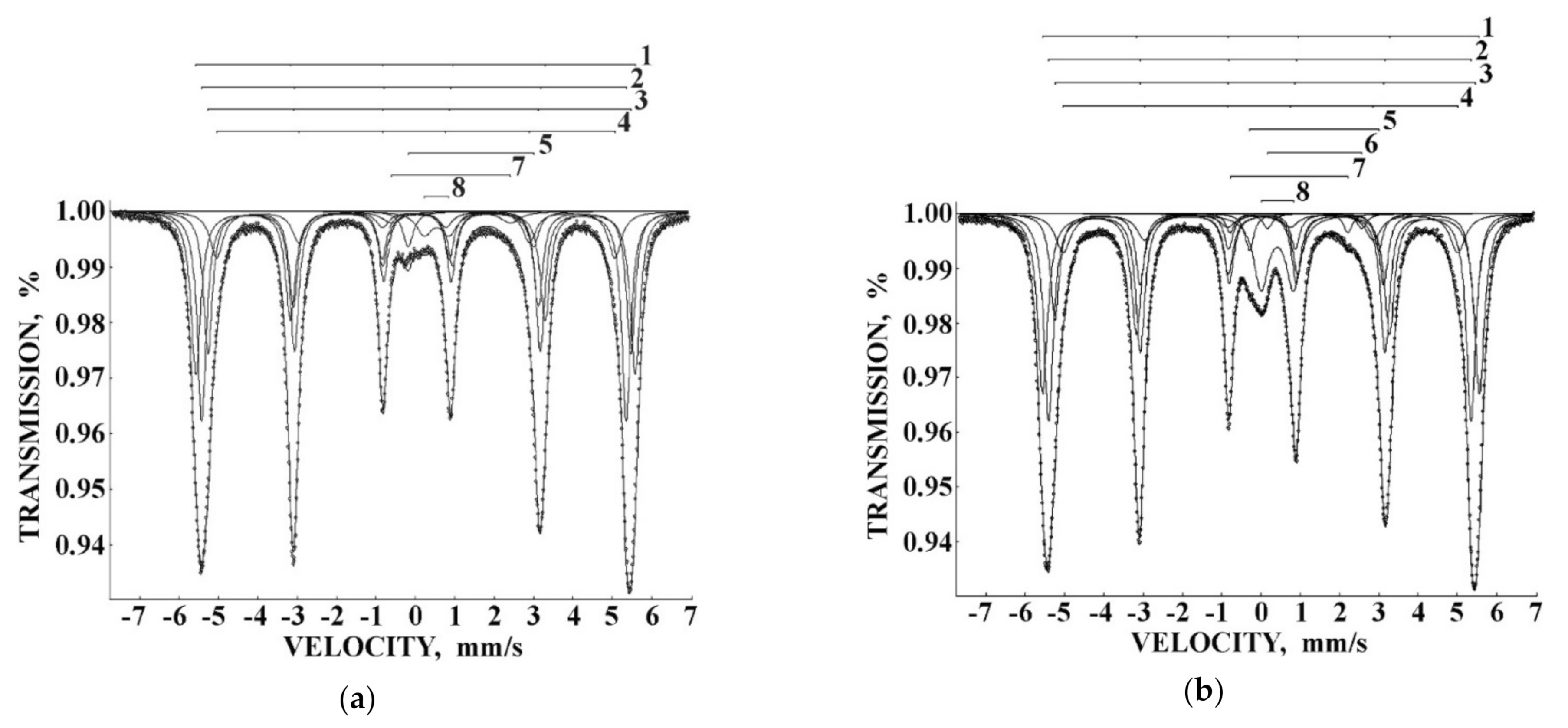
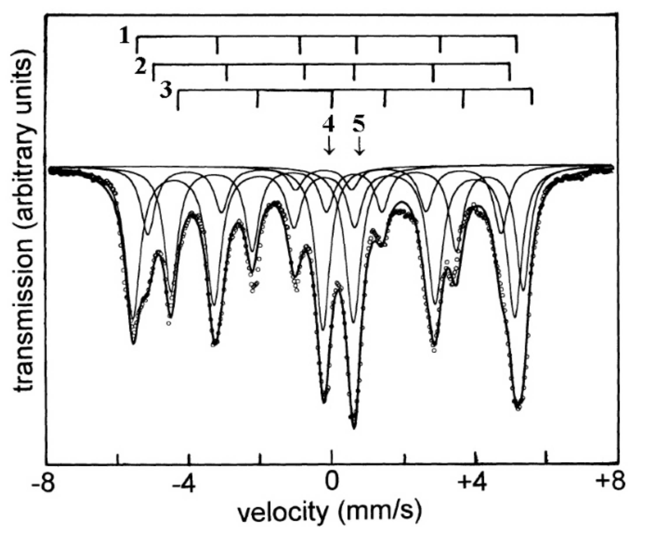
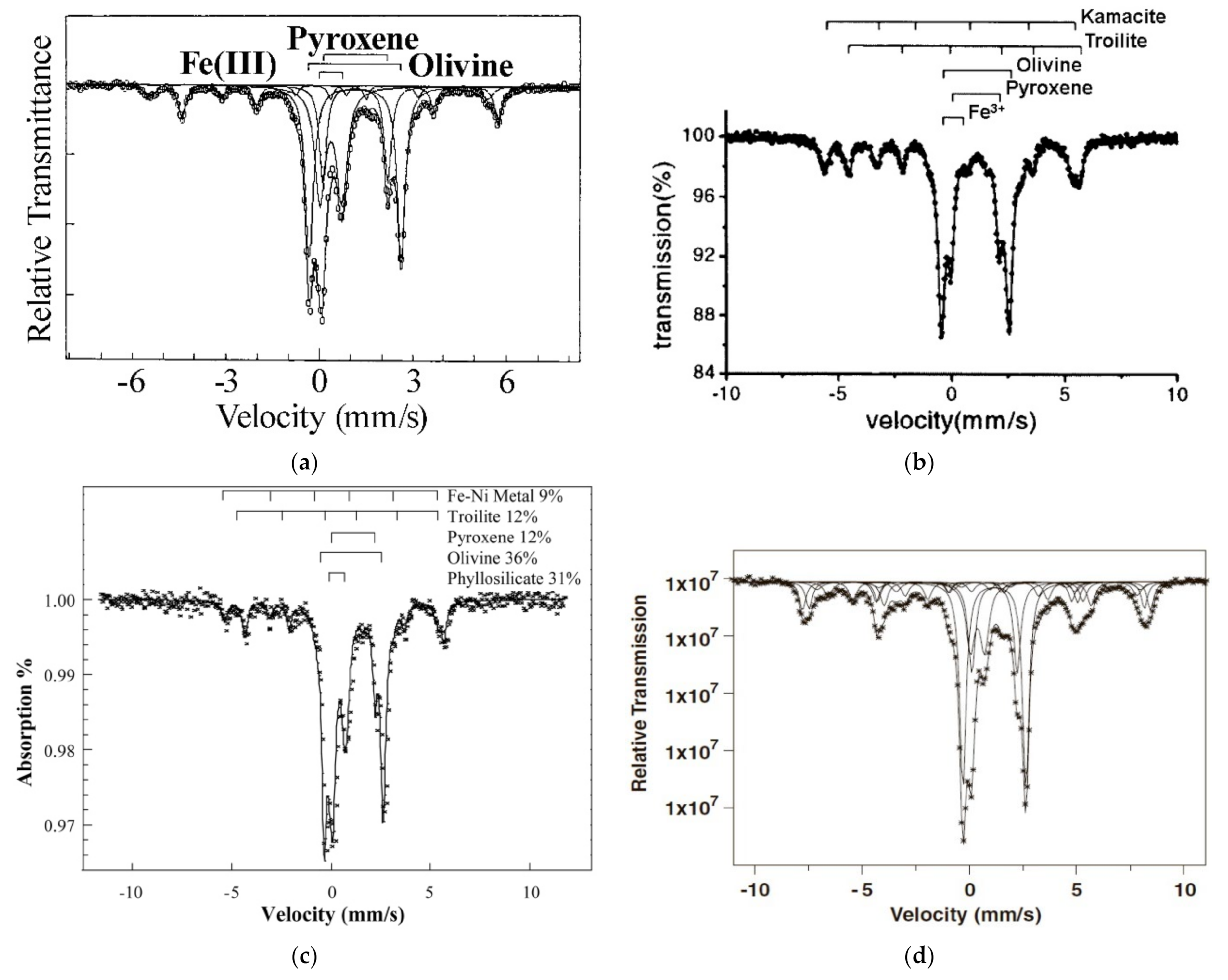
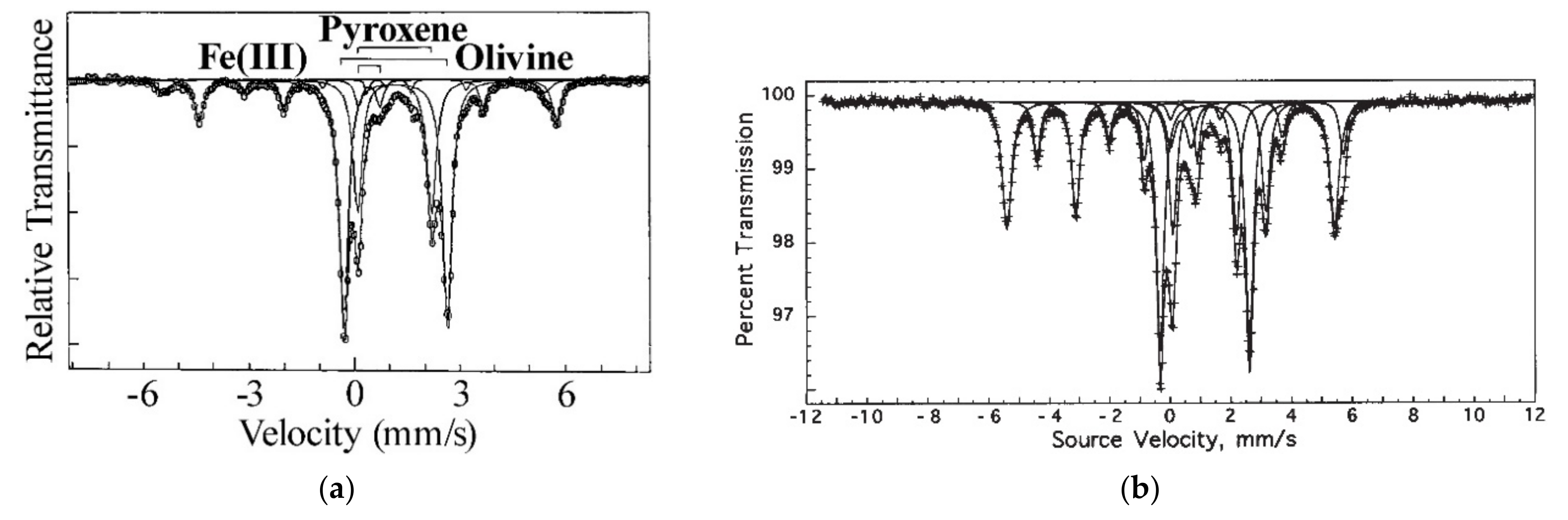
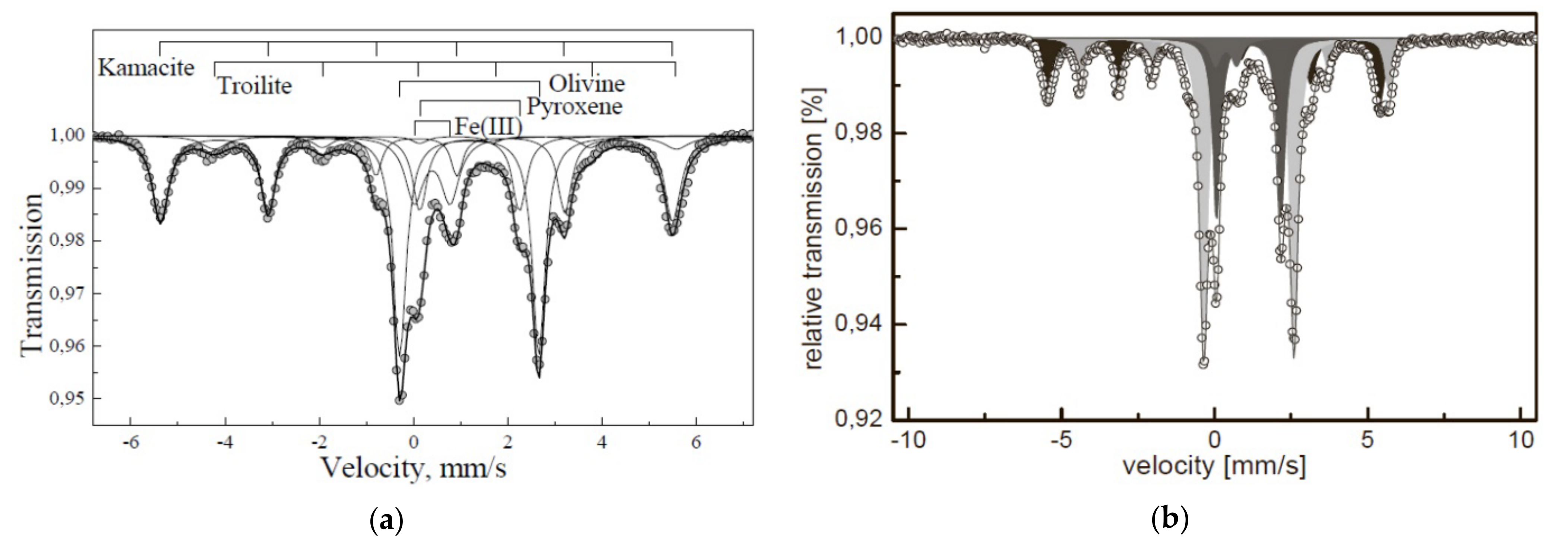
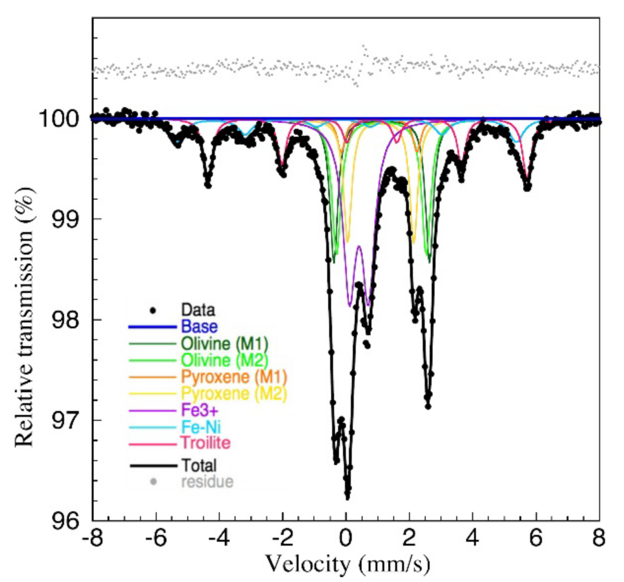
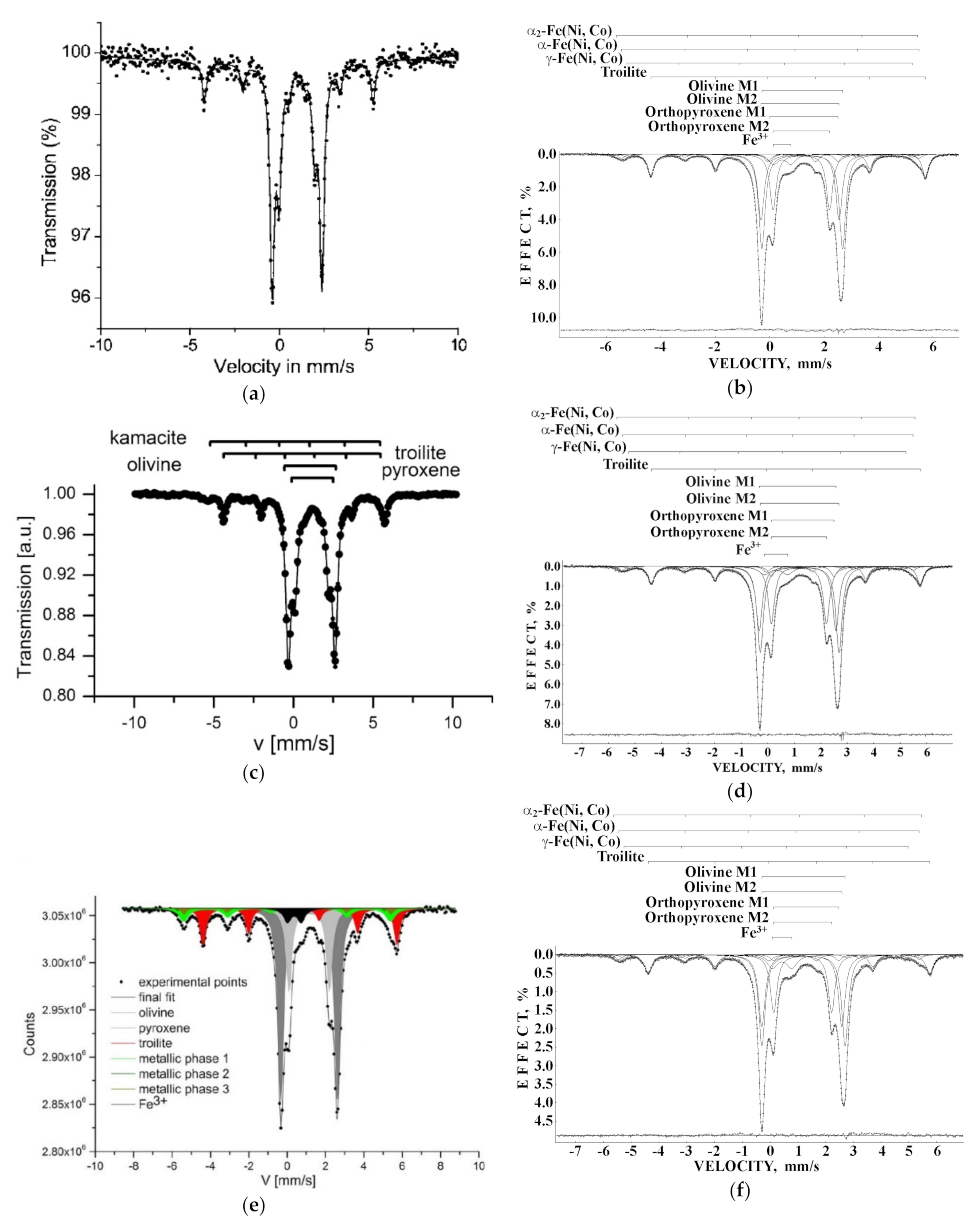
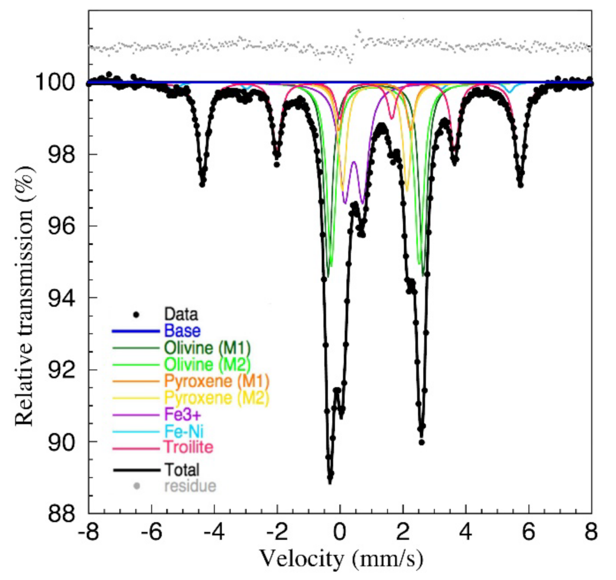
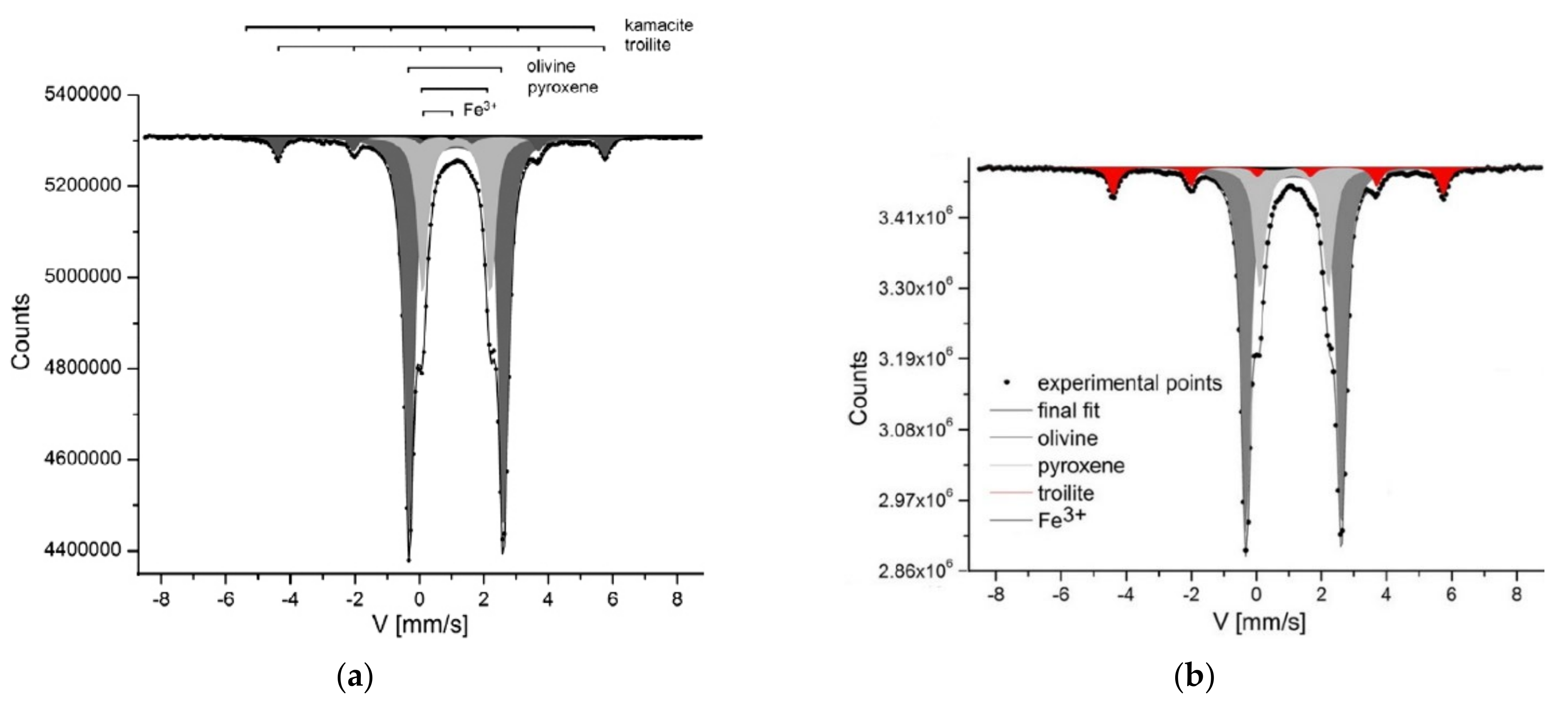
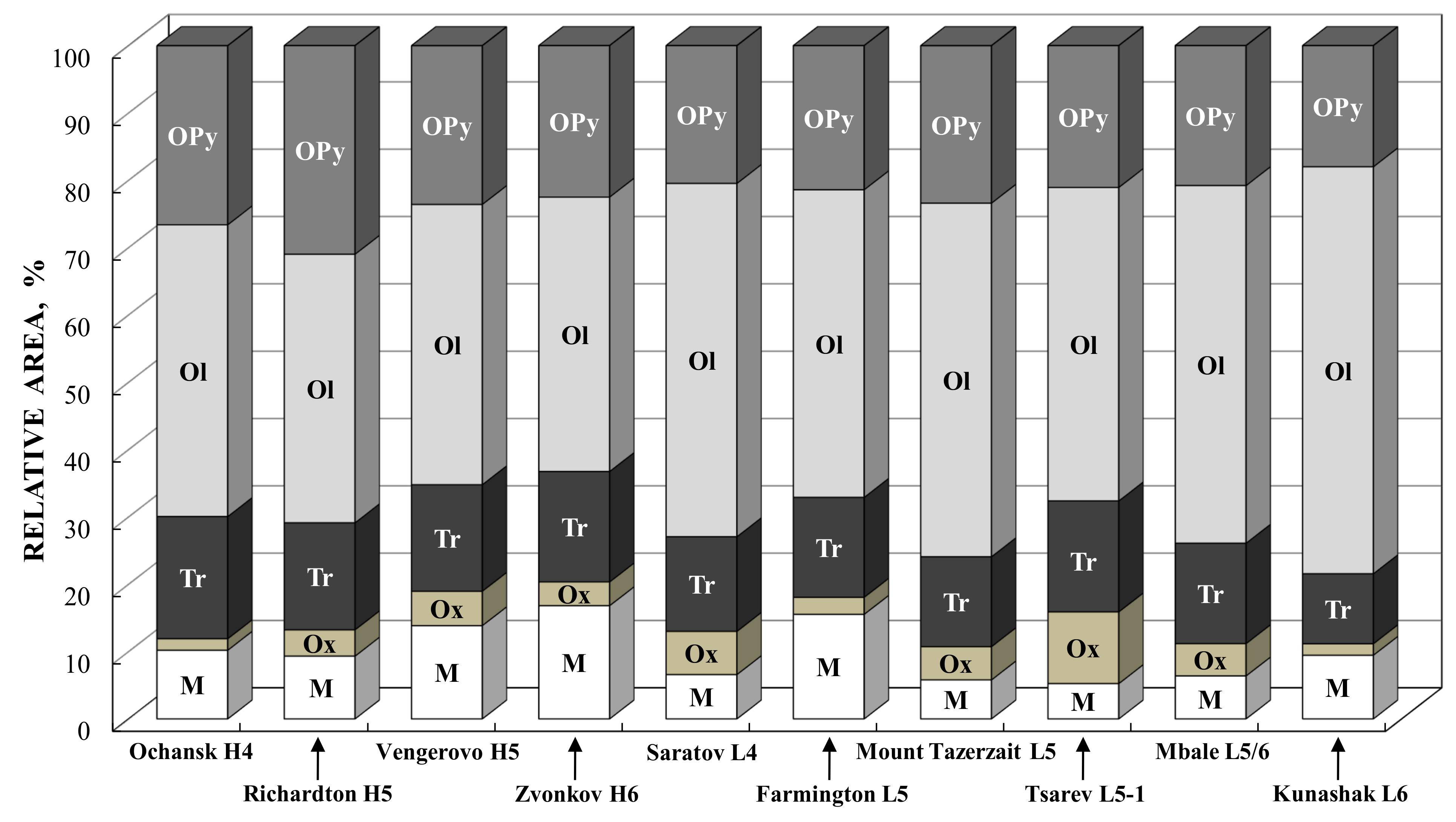
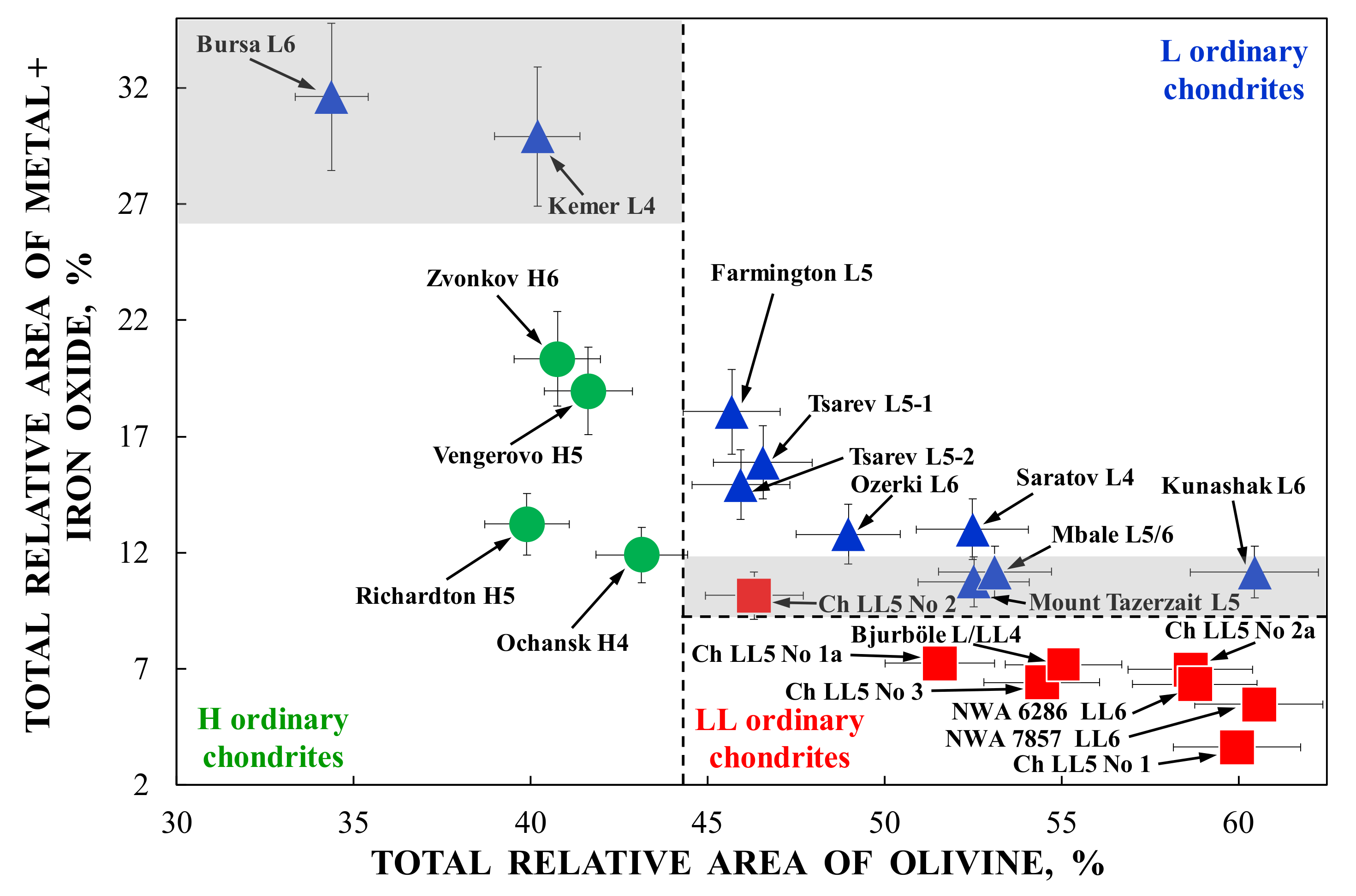
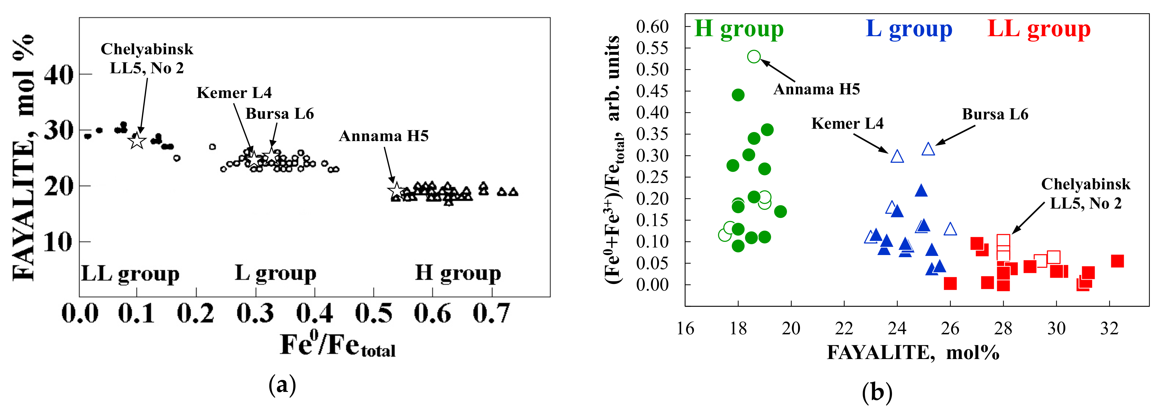
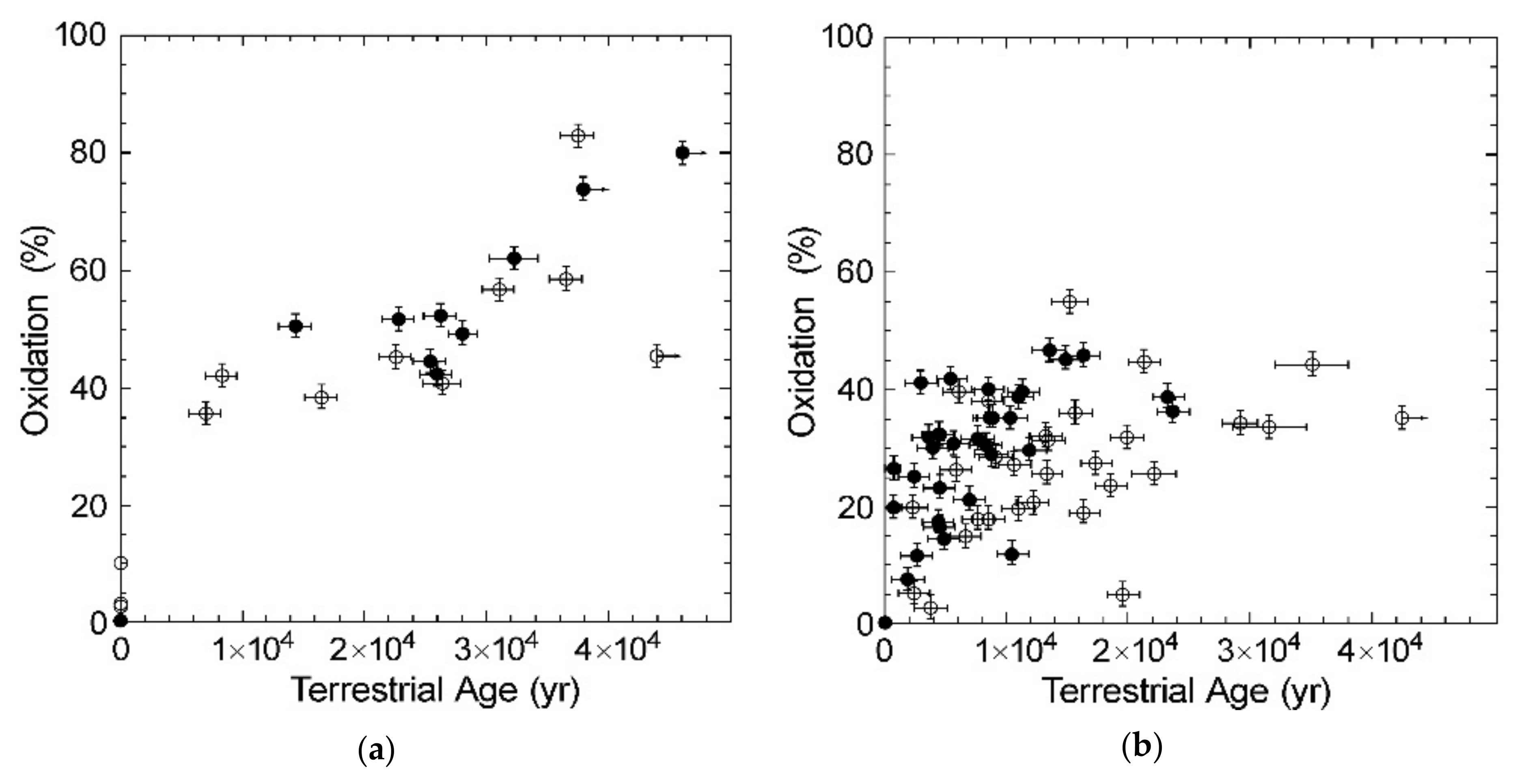
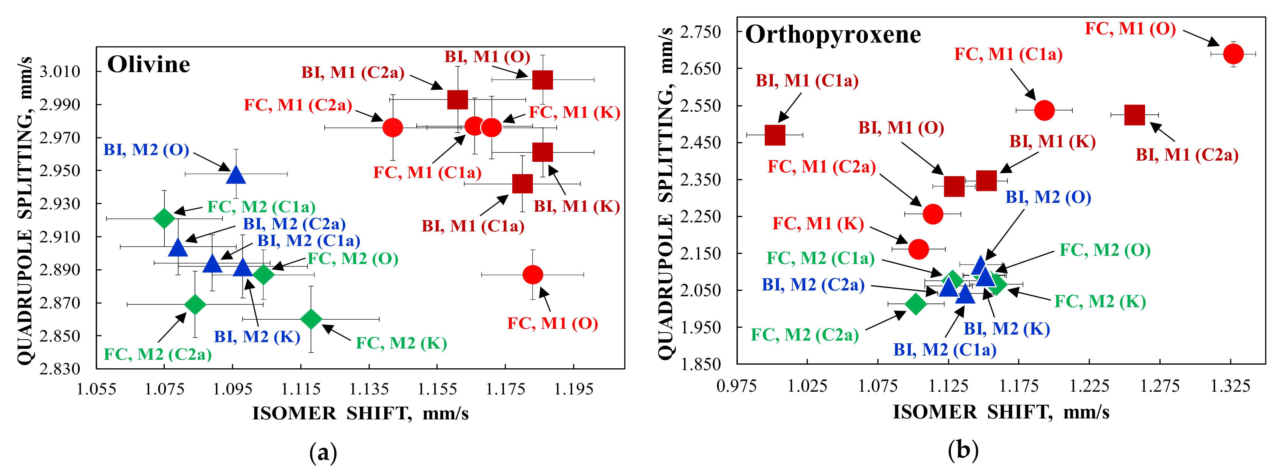
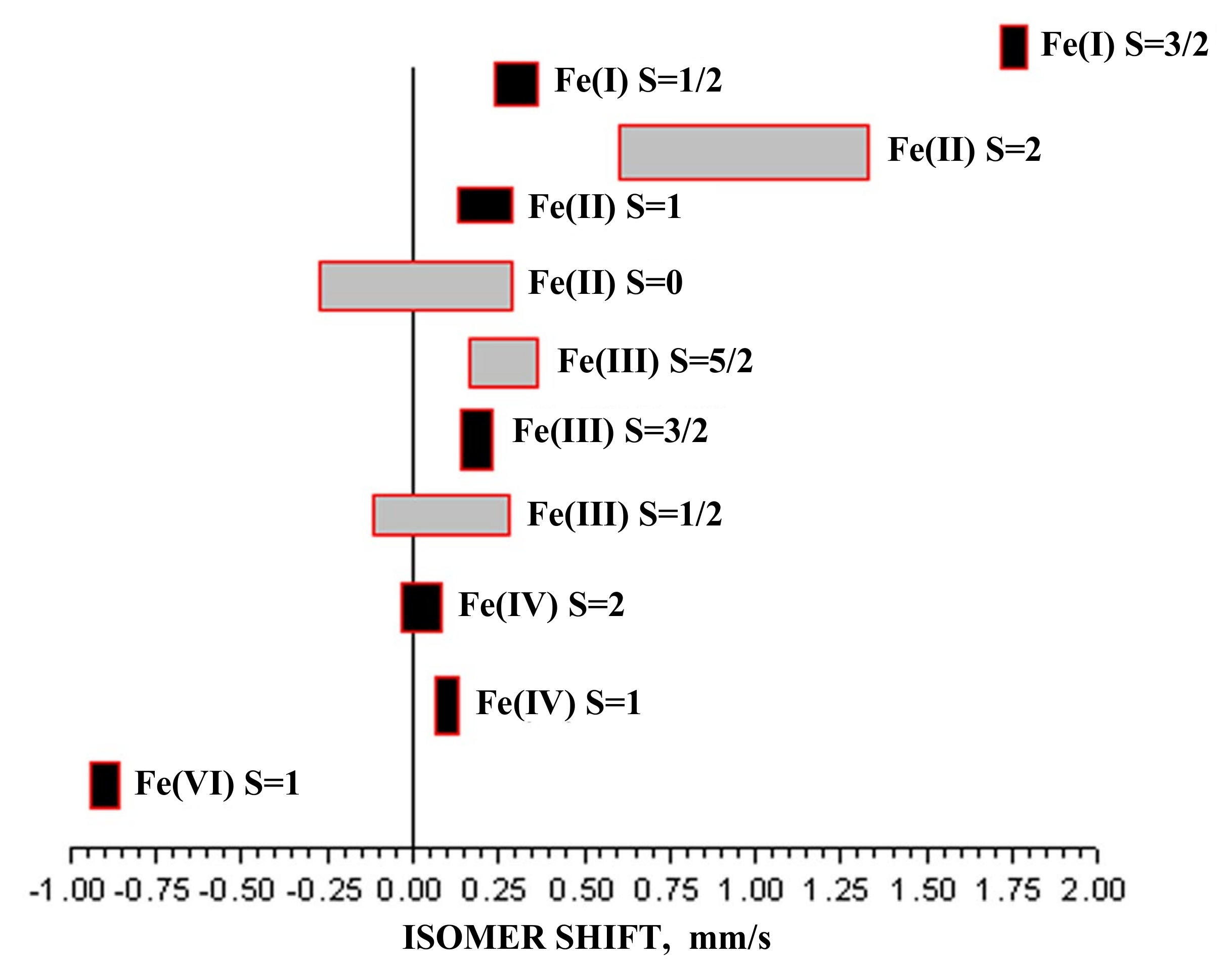
Table 1.
The ratios of Fe2+ fractions in the M1 and M2 sites in olivine, orthopyroxene and Ca-rich clinopyroxene crystals in ordinary chondrites determined by means of X-ray diffraction and Mössbauer spectroscopy (data were taken from References [100,101,107,112]).
| Silicate Crystals in Ordinary Chondrites | Method of Estimation | |
|---|---|---|
| XRD | Mössbauer Spectroscopy | |
| XFeM1/XFeM2 | AM1/AM2 | |
| Olivine | ||
| Ochansk H4 | – | 1.38 |
| Richardton H5 | – | 1.79 |
| Vengerovo H5 | – | 1.34 |
| Zvonkov H6 | – | 1.27 |
| Mount Tazerzait L5 | – | 1.34 |
| Farmington L5 | – | 1.47 |
| Kunashak L6 | – | 1.22 |
| Mbale L5/6 | – | 1.43 |
| Saratov L4 | – | 1.27 |
| Tsarev L5-1 | – | 1.29 |
| Annama H5 | 1.24 | 1.42 |
| Tsarev L5-2 | 1.36 | 1.44 |
| Kemer L4 | 1.56 | 1.55 |
| Bursa L6 | 1.37 | 1.35 |
| Ozerki L6 | 1.42 | 1.48 |
| Bjurböle L/LL4 | 1.21 | 1.24 |
| Chelyabinsk LL5, No 1 | 1.31 | 1.34 |
| Chelyabinsk LL5, No 1a | 1.21 | 1.21 |
| Chelyabinsk LL5, No 2 | 1.17 | 1.18 |
| Chelyabinsk LL5, No 2a | 1.32 | 1.37 |
| Chelyabinsk LL5, No 3 | 1.20 | 1.17 |
| NWA 6286 LL6 | 1.23 | 1.19 |
| NWA 7857 LL6 | 1.16 | 1.22 |
| Orthopyroxene | ||
| Ochansk H4 | – | 0.06 |
| Richardton H5 | – | 0.10 |
| Mount Tazerzait L5 | – | 0.17 |
| Farmington L5 | – | 0.15 |
| Kunashak L6 | – | 0.20 |
| Mbale L5/6 | – | 0.13 |
| Saratov L4 | – | 0.10 |
| Tsarev L5-1 | – | 0.09 |
| Annama H5 | 0.13 | 0.23 |
| Tsarev L5-2 | 0.20 | 0.19 |
| Kemer L4 | 0.15 | 0.13 |
| Bursa L6 | 0.31 | 0.28 |
| Ozerki L6 | 0.32 | 0.31 |
| Bjurböle L/LL4 | 0.23 | 0.28 |
| Chelyabinsk LL5, No 1 | 0.19 | 0.19 |
| Chelyabinsk LL5, No 1a | 0.18 | 0.33 |
| Chelyabinsk LL5, No 2 | 0.20 | 0.25 |
| Chelyabinsk LL5, No 2a | 0.26 | 0.40 |
| Chelyabinsk LL5, No 3 | 0.29 | 0.30 |
| NWA 6286 LL6 | 0.25 | 0.26 |
| NWA 7857 LL6 | 0.33 | 0.34 |
| Ca-rich clinopyroxene | ||
| Tsarev L5-2 | 1.28 | 1.50 |
| Kemer L4 | 3.00 | 3.02 |
| Bjurböle L/LL4 | 3.11 | 3.13 |
| Chelyabinsk LL5, No 1 | 2.54 | – |
| Chelyabinsk LL5, No 1a | 3.78 | 4.78 |
| Chelyabinsk LL5, No 2 | 1.78 | 1.90 |
| Chelyabinsk LL5, No 2a | 2.54 | 2.31 |
| Chelyabinsk LL5, No 3 | 2.43 | 2.33 |
| NWA 6286 LL6 | 1.33 | 1.30 |
| NWA 7857 LL6 | 2.00 | 2.43 |
Table 2.
The values of the distribution coefficient and the temperature of equilibrium cation distribution in olivine crystals in ordinary chondrites determined by means of X-ray diffraction and Mössbauer spectroscopy (data were taken from References [100,101,107,112]).
| Olivine Crystals in Ordinary Chondrites | Method of Estimation | ||||
|---|---|---|---|---|---|
| XRD | Mössbauer Spectroscopy | ||||
| KD | Teq, K | XFa | KD | Teq, K | |
| Ochansk H4 | – | – | 0.175 | 1.19 | 641 |
| Richardton H5 | – | – | 0.177 | 1.81 | 433 |
| Vengerovo H5 | – | – | 0.19 | 1.43 | 698 |
| Zvonkov H6 | – | – | 0.19 | 1.35 | 849 |
| Mount Tazerzait L5 | – | – | 0.246 | 1.47 | 654 |
| Farmington L5 | – | – | 0.238 | 1.65 | 503 |
| Kunashak L6 | – | – | 0.23 | 1.30 | 965 |
| Mbale L5/6 | – | – | 0.254 | 1.62 | 523 |
| Saratov L4 | – | – | 0.24 | 1.36 | 813 |
| Tsarev L5-1 | – | – | 0.243 | 1.40 | 744 |
| Annama H5 | 1.30 | 966 | 0.186 | 1.53 | 592 |
| Tsarev L5-2 | 1.52 | 602 | 0.243 | 1.59 | 542 |
| Kemer L4 | 1.77 | 441 | 0.24 | 1.77 | 439 |
| Bursa L6 | 1.50 | 623 | 0.252 | 1.50 | 625 |
| Ozerki L6 | 1.47 | 553 | 0.26 | 1.69 | 479 |
| Bjurböle L/LL4 | 1.46 | 666 | 0.262 | 1.34 | 850 |
| Chelyabinsk LL5 No 1 | 1.47 | 658 | 0.279 | 1.49 | 628 |
| Chelyabinsk LL5 No 1a | 1.29 | 979 | 0.279 | 1.30 | 964 |
| Chelyabinsk LL5 No 2 | 1.24 | 1179 | 0.279 | 1.25 | 1115 |
| Chelyabinsk LL5 No 2a | 1.48 | 645 | 0.279 | 1.55 | 573 |
| Chelyabinsk LL5 No 3 | 1.29 | 1002 | 0.279 | 1.25 | 1144 |
| NWA 6286 LL6 | 1.34 | 862 | 0.299 | 1.28 | 1006 |
| NWA 7857 LL6 | 1.24 | 1180 | 0.294 | 1.34 | 855 |
Table 3.
The values of the distribution coefficient and the temperature of equilibrium cation distribution in in orthopyroxene crystals in ordinary chondrites determined by means of X-ray diffraction and Mössbauer spectroscopy (data were taken from References [100,101,107,112]).
| Orthopyroxene Crystals in Ordinary Chondrites | Method of Estimation | ||||
|---|---|---|---|---|---|
| XRD | Mössbauer Spectroscopy | ||||
| KD | Teq, K | XFs | KD | Teq, K | |
| Ochansk H4 | – | – | 0.156 | 0.04 | 621 |
| Richardton H5 | – | – | 0.147 | 0.08 | 753 |
| Mount Tazerzait L5 | – | – | 0.208 | 0.12 | 879 |
| Farmington L5 | – | – | 0.205 | 0.10 | 823 |
| Kunashak L6 | – | – | 0.20 | 0.14 | 933 |
| Mbale L5/6 | – | – | 0.218 | 0.09 | 776 |
| Saratov L4 | – | – | 0.19 | 0.07 | 727 |
| Tsarev L5-1 | – | – | 0.20 | 0.06 | 677 |
| Annama H5 | 0.07 | 720 | 0.166 | 0.18 | 1035 |
| Tsarev L5-2 | 0.13 | 907 | 0.20 | 0.14 | 932 |
| Kemer L4 | 0.10 | 806 | 0.19 | 0.09 | 787 |
| Bursa L6 | 0.21 | 1138 | 0.214 | 0.21 | 1122 |
| Ozerki L6 | 0.24 | 1213 | 0.21 | 0.24 | 1202 |
| Bjurböle L/LL4 | 0.148 | 958 | 0.207 | 0.21 | 1136 |
| Chelyabinsk LL5 No 1 | 0.12 | 878 | 0.228 | 0.13 | 905 |
| Chelyabinsk LL5 No 1a | 0.14 | 942 | 0.228 | 0.25 | 1233 |
| Chelyabinsk LL5 No 2 | 0.13 | 908 | 0.228 | 0.17 | 1025 |
| Chelyabinsk LL5 No 2a | 0.18 | 1051 | 0.228 | 0.31 | 1416 |
| Chelyabinsk LL5 No 3 | 0.20 | 1107 | 0.228 | 0.22 | 1147 |
| NWA 6286 LL6 | 0.17 | 1010 | 0.239 | 0.18 | 1052 |
| NWA 7857 LL6 | 0.22 | 1169 | 0.242 | 0.25 | 1248 |
Table 4.
The ratios of the Fe2+ and Mg2+ occupancies among the M1 and M2 sites and the values of the distribution coefficient and the temperature of silicate crystals in the fusion crust (before fast cooling) from ordinary chondrites determined by means of X-ray diffraction and Mössbauer spectroscopy (data were taken from References [99,100]).
| Silicate Crystals in Ordinary Chondrites | Method of Estimation | ||||||
|---|---|---|---|---|---|---|---|
| XRD | Mössbauer Spectroscopy | ||||||
| XFeM1/XFeM2 | KD | TFC, K | AM1/AM2 | XFa/XFs | KD | TFC, K | |
| Ozerki L6 | |||||||
| Olivine | 1.19 | 1.25 | 1113 | 1.22 | 0.26 | 1.31 | 927 |
| Orthopyroxene | 0.22 | 0.16 | 978 | 0.21 | 0.21 | 0.15 | 962 |
| Kemer L4 | |||||||
| Olivine | 1.47 | 1.66 | 498 | 1.53 | 0.24 | 1.75 | 451 |
| Orthopyroxene | 0.19 | 0.13 | 901 | 0.14 | 0.19 | 0.09 | 803 |
Publisher’s Note: MDPI stays neutral with regard to jurisdictional claims in published maps and institutional affiliations. |
© 2021 by the authors. Licensee MDPI, Basel, Switzerland. This article is an open access article distributed under the terms and conditions of the Creative Commons Attribution (CC BY) license (https://creativecommons.org/licenses/by/4.0/).
Share and Cite
MDPI and ACS Style
Maksimova, A.A.; Oshtrakh, M.I. Applications of Mössbauer Spectroscopy in Meteoritical and Planetary Science, Part I: Undifferentiated Meteorites. Minerals 2021, 11, 612. https://doi.org/10.3390/min11060612
AMA Style
Maksimova AA, Oshtrakh MI. Applications of Mössbauer Spectroscopy in Meteoritical and Planetary Science, Part I: Undifferentiated Meteorites. Minerals. 2021; 11(6):612. https://doi.org/10.3390/min11060612
Chicago/Turabian StyleMaksimova, Alevtina A., and Michael I. Oshtrakh. 2021. "Applications of Mössbauer Spectroscopy in Meteoritical and Planetary Science, Part I: Undifferentiated Meteorites" Minerals 11, no. 6: 612. https://doi.org/10.3390/min11060612
Note that from the first issue of 2016, this journal uses article numbers instead of page numbers. See further details here.