Article

Reconstructing a Three-Dimensional Geological Model from Two-Dimensional Depositional Sections in a Tide-Dominated Estuarine Reservoir: A Case Study of Oil Sands Reservoir in Mackay River, Canada

1
Research Institute of Petroleum Exploration and Development, CNPC, Beijing 100083, China
2
China National Oil and Gas Exploration and Development Company, Beijing 100034, China
3
Key Laboratory of Oil and Gas Resources and Exploration Technology, Ministry of Education, Yangtze University, Wuhan 430100, China
4
School of Geosciences, Yangtze University, 111 University Road, Caidian District, Wuhan 430100, China
*
Authors to whom correspondence should be addressed.
Minerals 2022, 12(11), 1420; https://doi.org/10.3390/min12111420
Submission received: 8 October 2022 / Revised: 28 October 2022 / Accepted: 3 November 2022 / Published: 9 November 2022

Abstract

:
A tide-dominated estuarine reservoir is an important oil reservoir. However, due to the force of bidirectional water flow, its internal structure is complex, and the heterogeneity is serious. Accurately establishing the tide-dominated estuarine reservoir model is a great challenge. This paper takes the Mackay River oil sands reservoir in Canada as the research object to establish the elaborate geological model of a tide-dominated estuarine reservoir. Through the meticulous depiction of core data, 14 kinds of lithofacies and nine kinds of architectural elements are identified, and the lithological and electrical response in sedimentary architectural elements is established. On this basis, the plane and vertical distribution of architectural elements, as well as the spatial superimposition patterns, are depicted and characterized through well seismic combination and plane and section interaction, and the representative plane and section architecture maps are obtained as 2D training images (TIs) for multi-point statistical modeling. The 2D TI is scanned by 2D data template to obtain the multi-point statistical probability of the 2D spatial architectural pattern. Then, the 2D multi-point probability is fused to generate three-dimensional (3D) multi-point statistical probability by the probabilistic fusion. Finally, Monte Carlo sampling is used to predict the spatial distribution of architectures, and an elaborate geological model of a tide-dominated estuarine reservoir is established. Compared with the traditional sequential indication modeling method, the point-to-point error of the model section based on the 2D section reconstruction method is only 25.92%, while the sequential indication modeling method is as high as 58.52%. Even far from the TI, the point-to-point error of the 2D section model is 33.13%. From the cross-validation, the average error of the 2D section is 11%, while the sequential indicator modeling error is 23.1%, which indicates that the accuracy of 2D reconstruction of the estuarine reservoir model is high, and this method is suitable for the establishment of the tide-dominated estuarine reservoir model.

1. Introduction

An estuary is a very important transitional sediment environment, which develops in the transgression period where rivers enter the sea and receive sediments from both the river and the sea. They are mostly shaped like horns or funnels. Estuarine deposition is closely related to human activities and oil exploration. Typical modern tide-dominated estuary sediments include Fundy Bay [1], Fitzroy River Estuary [2,3], Severn River Estuary, etc. In recent years, estuarine reservoirs have also been found in the ancient stratigraphic records of Oriente Basin [4] and Abu Gharadig Basin [5], which contain a large amount of oil and gas, making estuarine reservoirs an important field for hydrocarbon geologists.
Mackay River sand reservoir of McMurray Formation is considered a typical ancient tide-dominated estuary sediment; it contains huge deposits of oil sands but is influenced by the complex hydrodynamic, estuary open angle, paleo-geomorphology and sea level changes. It also has lots of problems such as advanced heterogeneity, complex reservoir sand body superposition style and internal structure, which introduces a great challenge to reservoir prediction. Previous studies on estuarine reservoirs have been carried out through depositional numerical simulation [6], modern deposition [1,2,3,7], hydrodynamic dynamics [8], reservoir architectural elements [9,10,11] and other aspects revealing the internal structure and superposition style of estuarine reservoirs, but the establishment of reservoir models to predict the spatial distribution is relatively rare [5,12,13]. Traditional geological modeling methods, such as the two-point statistical method based on variation function, make good use of the existing geological information, but they are insufficient in the reservoir morphology and architecture superposition style, and the established tidal estuarine reservoir model is relatively simple and has limited predictability. Object-based modeling methods are still poor for dense well data processing. Due to the shallow burial and high seismic resolution of the Canadian oil sands, it is possible to combine geology and seismic data to trace architectural elements. However, this tracking and carving work is extremely arduous, and due to the small scale of architectural elements and little interface difference, there is large uncertainty in seismic identification. The reliability of a 3D model obtained by direct seismic interpretation is low, which is not conducive to model risk analysis. Recently, a group of scholars conducted a 3D modeling study of the estuary reservoir through depositional numerical simulation combined with multi-point geostatistics [13]. The core idea is to obtain 3D TIs by depositional numerical simulation to solve the demand for 3D TIs in multi-point geostatistics. However, it is very difficult to obtain the deposition kinetic parameters that are similar to those of underground deposition, so the representativeness of the obtained TIs is questionable. Although multi-point geostatistics has been studied for more than 30 years, a difficult problem in its popularization and application is the acquisition and evaluation of 3D TIs. Many scholars obtain TIs from sedimentary process simulation, object-based modeling, flume experiments, ground-penetrating radar and satellite data, as well as seismic data interpretation. However, the number of TIs is small and cannot meet the needs of practical applications. Secondly, the degree of conformity between the TIs and the actual block needs to be evaluated, and the quality of the model depends considerably on the representativeness of the input TIs. Thirdly, the existing TIs acquisition methods mainly focus on fluvial facies, and the TIs of other sedimentary systems, especially estuarine reservoirs, are rarely studied. Therefore, the establishment of a 3D model of tide-dominated estuarine reservoir is a key problem in reservoir prediction.
To avoid the problem of obtaining multi-point geostatistical representative 3D TIs, scholars attempted to reconstruct 3D geological models from 2D geological sections as TIs. Okaba (2004, 2005) used rock slices to construct a 3D pore-throat network model in the multi-point modeling of rock microscopic pore-throat [14,15]. However, the premise is that the distribution of pore-throat in rock is homogeneous, which has been improved by many scholars to express pore-throat’s heterogeneity. On this basis, Comunian (2012) extended it to lithofacies simulation, which attracted the interest of reservoir architecture modeling researchers, and gradually improved and formed the method of 3D reservoir geological model reconstruction based on 2D geological sections (2D to 3D) [16]. The advantage is that the TIs are directly derived from the architectural dissection of the reservoir and are satisfied with the data of the actual study area. Therefore, the TIs are representative. As the TIs are scanned through 2D multi-point data templates, the reservoir architecture and morphology information reflected in the 2D sections can be well captured. The 3D reservoir architecture and shape are well reproduced by the fusion of 2D sections in multiple directions. In this paper, based on the elaborate dissection of the reservoir architecture, the method of reconstructing a 3D model by 2D sections is adopted to establish the estuary reservoir model, which provides model support for a deep understanding of the heterogeneity in the tide-dominated estuary, as well as provides a reference for the establishment of the fine model of reservoirs in a similar environment.

2. Geological Setting

The Alberta Basin is located between the Canadian Shield and the Rocky Mountains. It is a typical foreland basin with narrow strip distribution and an NW-SE trend. The Alberta Basin is rich in oil sands, among which Athabasca oil sands are the most abundant [17]. Most bitumen resources in the Athabasca oil sands are located in the Lower Cretaceous McMurray Formation. The overall lithology of the McMurray Formation is mainly sandstone and sand–mudstone interbedded. Carrigy (1959) subdivides the McMurray Formation into the Upper, Middle and Lower member according to lithologic characteristics: Lower McMurray, Middle McMurray and Upper McMurray from bottom to top [18]. The Upper and Middle McMurray are stable, while the Lower McMurray is generally absent.
The McMurray Formation in the study area is a third-level sequence as a whole, and only transgression and highstand systems are developed in the study area [19]. Corresponding to the Middle and Upper McMurray Formation, the formation development style of multiple incised erosion and filling is formed under the overall long-term transgression and multiple medium-term and short-term regression–transgression [20]. When the McMurray Formation was deposited, it gradually changed from fluvial to coastal facies from the Lower member to the Upper member. Sandstone in the Middle McMurray Formation is filled in a super-large incised valley on the second-order sequence interface, forming a tidal flat and estuary system. Under the background of the east–west extrusion of the foreland basin, due to the continuous rise and short-term decline in relative sea level, a multi-stage incised valley appeared in the McMurray Formation, forming the pattern with high-frequency incised and filled stratum development.
The study area (Figure 1) covers an area of about 1360 km2 with abundant data, including the well-logging data of 281 conventional wells, core data of 168 coring wells, grain size data of 67 wells, dip data of 36 wells and 3D seismic data of more than 30 km2. It provides sufficient data support for the establishment of an accurate 3D geological model.

3. Geological Dissection of Tidal Estuarine Reservoir

Through previous studies [11,21] and observation of core in the study area, the study area is known to have tide-dominated estuary deposition, and tidal bar is an important reservoir. Tidal bars with reverse grain sequence (Mutti et al., 1985) [22] are developed longitudinally in tide-dominated estuaries, and they are usually large composite sand bodies with lateral accretion rather than vertical accretion [23].

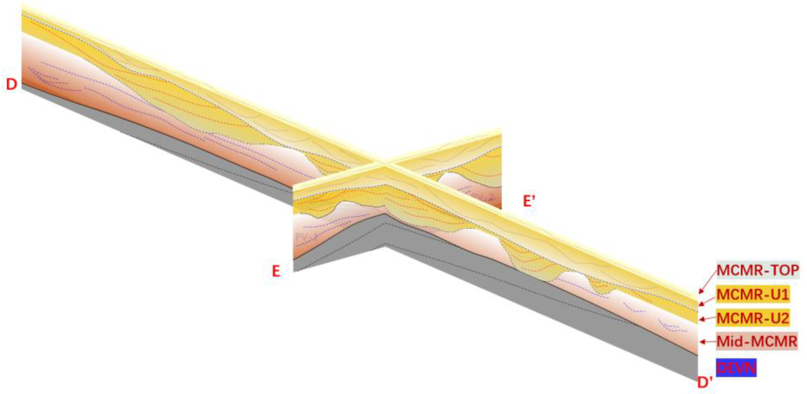
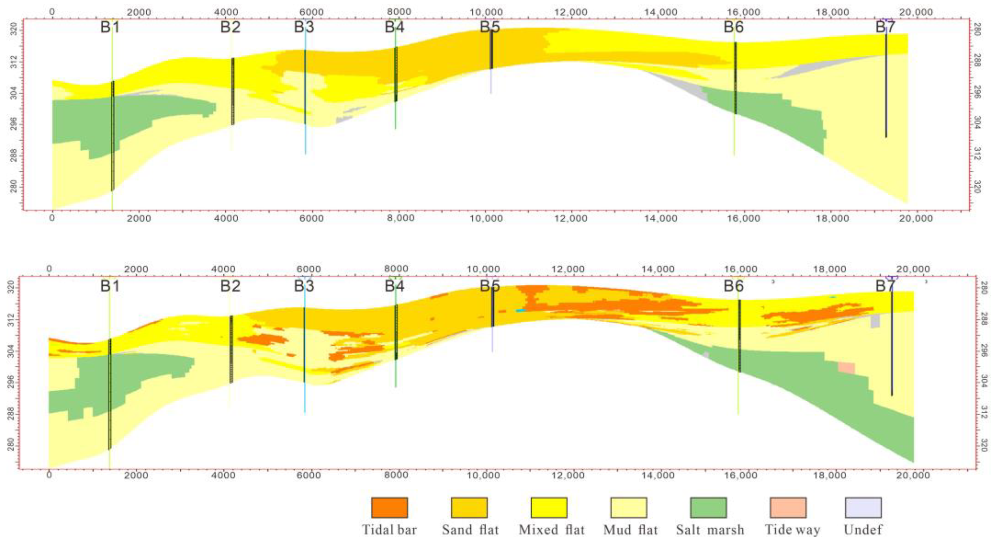
3.1. Stratigraphic Division and Correlation

The McMurray Formation is divided into the Middle and Upper members by analyzing the seismic response characteristics and log pattern, combined with lithologic data for stratigraphic correlation and division. The Middle McMurray exhibits a weak reverse rhythm with a high GR value and low resistivity. It is deposited in the estuarine coastal plain or inner-middle estuarine, and the content of the mud interlayer is high. The Upper McMurray shows a low GR value, high resistance, low mud interlayer content and good stratification. The Middle McMurray is deposited on the carbonate basement of Devonian (DEVN), which is dominated by the paleo-gully topography of the basement, showing a style of filling and complementing. The Upper McMurray is the main oil-bearing reservoir. To conduct fine modeling and characterization of the reservoir, the Upper McMurray is subdivided into four small layers, namely, U2, U1-2, U1-1 and TOP (Figure 2). In the McMurray Formation, there are several incision and filling processes, with the Upper section eroding the estuary and coastal mudstone deposits in the Middle section and filling the thick sandstone. The effect of bottom-up incision in the Upper segment has gradually weakened, and the phenomenon of U1-1 incision in the Upper segment is hardly visible. On the whole, the McMurray Formation is a period of transgression interleaved with high-frequency short-term regressive processes; the sedimentary system has receded to the land, and the river incision is weakened.

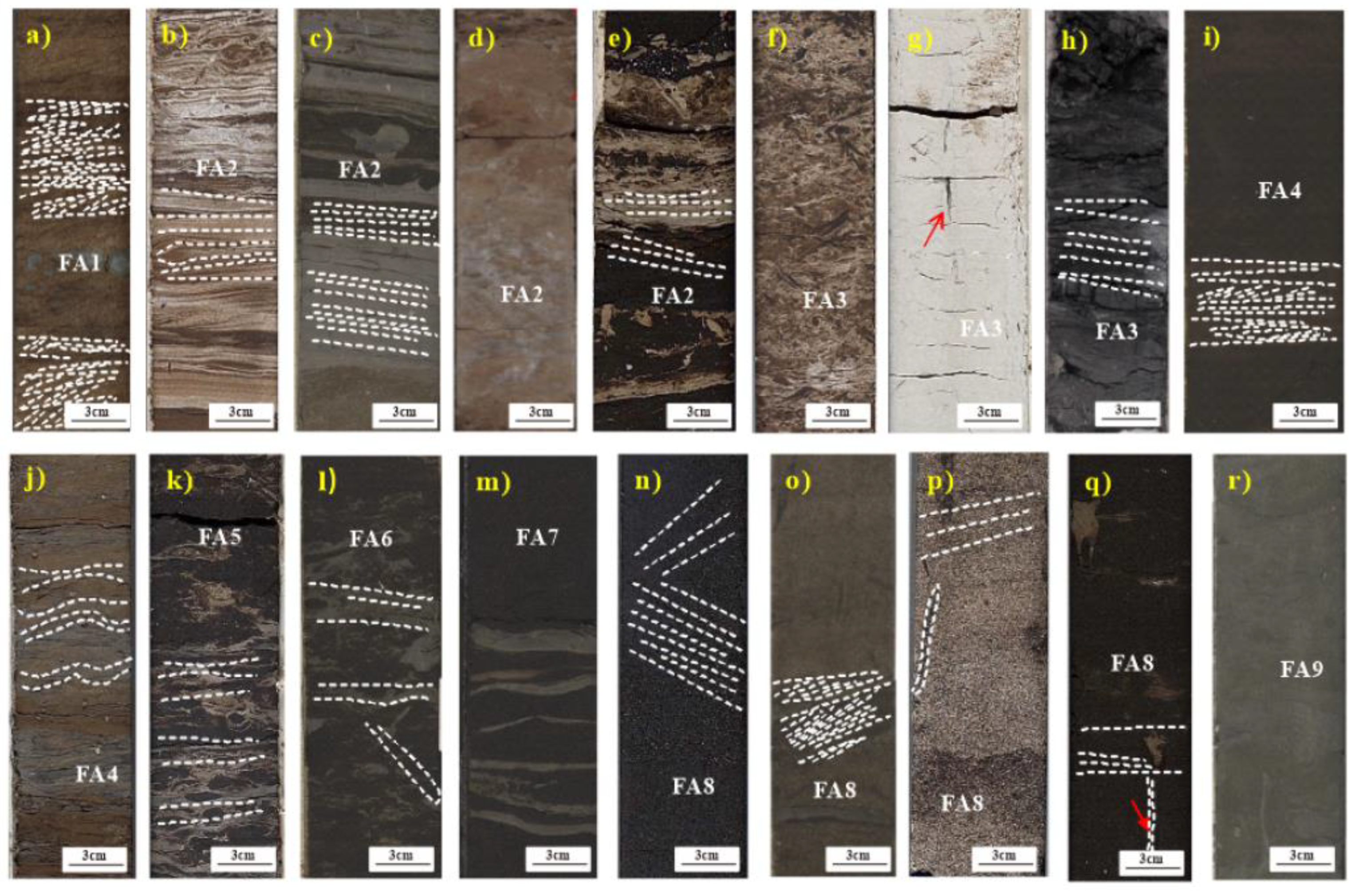
3.2. Architectural Elements

According to the characteristics of the core, such as color, grain size, sedimentary structure and biological disturbance, 14 types of lithofacies are identified. Nine architectural elements are recognized according to the lithofacies associations (Figure 3). The Middle McMurray mainly comprises FA1–FA4, namely, sandy channel filling, point bar, salt marsh, and tidal channel point bar; the Upper McMurray is mainly composed of FA5–FA9, which are mud flat, mixed flat, sand flat, tidal bar and offshore, respectively. Mud flat, mixed flat and sand flat constitute tidal flat [24]. Tidal flat and tidal bar constitute the main architectural elements, among which tidal bar and sand flat are the superior reservoirs.

3.2.1. FA1: Sandy Channel Filling

FA1 is fine sandstone with herringbone cross-bedding and tabular cross-bedding, and it has strong biological disturbance. The content of mud is small, and occasionally, rock debris and mud particles are found at the bottom. The bottom has a scour surface. The logs are reverse rhythm, GR and resistivity are high, and SP is close to the baseline.

3.2.2. FA2: Point Bar

FA2 is a lenticular-to-wavy sandy mudstone interbedded with wavy and lenticular bedding. The lithology is uneven including collapsed mud conglomerates. There are biological remains. FA2 is a slanted heterogeneous sand–mud interbed, which is formed in an environment where water flow varies greatly. It has a weak positive rhythm with high GR value with a toothing shape, and its SP curve is close to the baseline with low resistivity.

3.2.3. FA3: Salt Marshes

FA3 shows plant root traces and massive brittle coal seams, indicating the continuous deposition and vertical accretion of sediments in a moist, low-energy salt marsh environment. It has a weak reverse rhythm, high Gr value and resistivity, and its SP curve is close to the baseline.

3.2.4. FA4: Point Bar in Tidal Channels

FA4 is dominated by small-angle parallel bedding and wavy bedding, followed by flaser bedding, and the bio-disturbance shows sporadic heterogeneous distribution. It has a weak reverse rhythm with high GR and resistivity, and its SP curve is close to the baseline. The point bar of the tidal channel is tidal deposits. At high tide, the tidal channel is filled with water, and the point bar in tidal channels is deposited on its sides, presenting lenticular bedding. The point bar is deposited in meandering rivers with inclined heterolithic stratification and a high mud content.

3.2.5. FA5: Mudflat

FA5 has mainly developed wavy bedding, and heavy biological disturbance has destroyed the mud–sand interbedded structure with less biological disturbance, higher mud content and silt. There are different proportions of bio-disturbed interbedded sand, silt and mudstone, and scattered shell fragments, organic debris and coal debris. It has a weak positive rhythm with middle GR and resistivity, and its SP curve is far from the baseline.

3.2.6. FA6: Mixed Flat

FA6 has parallel bedding and wavy bedding with a high mud content, and most of the mud is strongly bioturbated. Mixed flats and mud flats often develop together. The difference lies in the level of mud content, which is formed under the tidal environment with alternating strong and weak hydrodynamic forces. It has a positive rhythm, which has low GR with less fluctuation, low resistivity, and an SP curve away from the baseline.

3.2.7. FA7: Sand Flat

This is black, fine-grained sandstone with parallel bedding and herringbone cross-bedding, and the bioturbation is of sporadic heterogeneous distribution. Under the action of a high-speed tidal current, the sandy flat is a sandy deposit under a high-energy hydrodynamic environment; it is a transverse-accreted bar deposit at the edge of a shallow bay, where tides are dominant. The reverse rhythm is dominant, GR is low, resistivity is high, and the SP is far from the baseline.

3.2.8. FA8: Tidal Bar

The sedimentary structure with large tabular cross-bedding and herringbone cross-bedding reflects the high-energy sedimentary environment. The tidal bars are reverse rhythmic, which are usually large composite sand bodies with lateral accretion. The reverse rhythm is dominant, GR is extremely high, resistivity is high, and SP is far from the baseline.

3.2.9. FA9: Offshore

This is the far-shore deposition of mixed tidal action influenced by waves. The deposition is very slow and stable in the whole area. Distinct glauconite sand is visible, indicating an open marine environment. The high degree of biological modification makes it easy to homogenize with sandstone. GR is extremely jagged with low resistivity and SP is close to baseline.

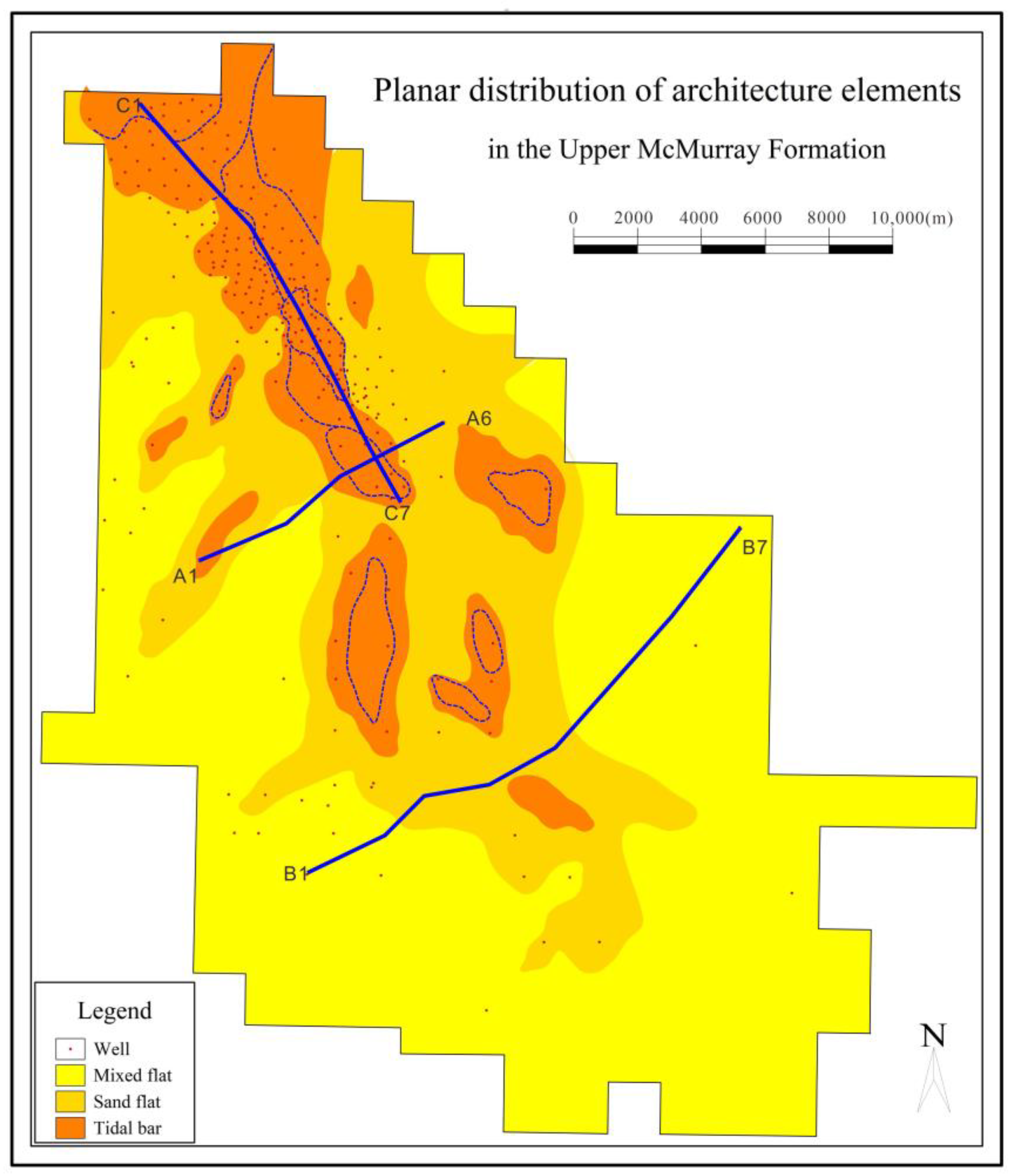
3.3. Reservoir Architecture

Guided by Miall’s analysis method of reservoir architectural elements, two cross-sections and one longitudinal section of the main sedimentary area (Figure 4) with seismic data are selected for architecture dissection. The architecture of the main tidal bar was dissected with seismic reflection style as constraint, logging response feature identification and rock correlation analysis, and well seismic combination.
On the seaward cross-section 1 (Figure 5), the boundary, superposition style and internal characteristics of architectural elements are determined by seismic reflection features, and the types of architectural elements are determined by combining the characteristics of lithofacies. Middle McMurray is poorly preserved and has developed salt marshes, mud flats and other deposits; the formation is generally flat inside. Upper McMurray is incised, and most architectural elements include lateral splicing contact and have lateral accretion. Mud flat is developed at the bottom of McMurray U2, and mixed flat is developed at the top. The two are vertically spliced and contacted, generally flat, and the interior is nearly parallel. McMurray U1-2 developed a mixed flat, sand flat, mud flat complex and tidal bar complex, showing small-scale lateral erosion-filling deposition. McMurray U1-1 developed sand flats and tidal bars, which deposited in the incised valley and above the sand flats with high-angle continuous lateral accretion.
Cross-section 2 (Figure 6) is closer to land and far from the seismic zone, so its architecture was dissected mainly ba5sed on lithologic data and logging data. From north to south, the incised degree of Middle McMurray is weakened, and the erosion degree of cross-section 2 is also weakened. Only the middle strata are eroded away. The middle member on the east and west sides are well preserved with salt marshes and point bars. The incision degree of Upper McMurray becomes moderate, the mud flat and mixed flat in U2 show vertical splicing contact, while sand flat, mixed flat and mud flat are mostly lateral splicing contact in U1 member.
Compared with two cross-sections, the McMurray Formation changes from thick to thin from the land to sea direction, the degree of stratum retention changes from good to poor, the depth of incised valley changes from shallow to deep, and the incised range changes from narrow to wide and large. Sand flat and tidal bar is the main reservoir, which is distributed in the middle incised valley with the sea level changing many times. The sedimentary associations with multiple incisions and filling are formed. Tidal bar and sand flat are lateral accretions, and there is a lateral lithofacies gradient; the lateral end was filled with sand flat and mixed flat.
The distribution relationship and internal structure of architectural elements are analyzed according to the longitudinal section (Figure 7). There are local remnants in Middle McMurray, and its preservation is very poor. McMurray U2 is thin in the north and thick in the south due to incised filling, and the dip of the sand flat is in the southward direction. The layer of McMurray U1-2 is thick in the north and thin in the south due to incised erosion, and the dip of the tidal bar is in the southward direction. In McMurray U1-1, tidal bars have developed continuously along the longitudinal direction, but the lithofacies show gradual changes. The downstream direction is mainly filled with deep valley sediments, including tidal bar and sand flat. Estuarine coastal plain and inner-middle estuary in the middle part of the McMurray Formation are mainly deposited in the upstream direction, while the Upper McMurray formation is thin and limited in scale.
Through the cross and longitudinal section, the Middle McMurray is of estuarine and coastal deposition with erosion residue, while the Upper McMurray is filled with a large incision system, and mud flat, mixed flat, sand flat and tidal bar are developed from bottom to top. There are many point bars and salt marshes in the Middle McMurray, and occasionally, channel filling deposits are found. In the Upper McMurray, most of the architectural elements show lateral splicing contact, while the mud flat and mixed flat have gentle accretion. The high-angle continuous accretion can be seen in the sand flat and tidal bar. The Upper McMurray is mainly tidal flat in U2, and sandy flat and tidal bar in U1.
In the cross-section, the incised valley combines with the outer estuary from south to north to form a shallow-to-deep landform, and the tidal flat and tidal bar gradually widen. The development of the tidal bar is closely related to the vertical erosion caused by the changes in sea level and the geomorphology of the estuary. In the longitudinal section, it is dominated by a deep valley filled with sediments downstream, mainly including tidal bar and sand flat. Estuarine coastal plain and inner-middle estuary in the Middle McMurray are mainly deposited in the upstream direction, while the Upper McMurray is thin and limited in scale.
Based on the architectural analysis, the plane architectural element is analyzed (Figure 4). Under the background of the filling and deposition of a large incision system, a large tidal bar complex developed on the northern side of the sea, which was laterally deposited and filled in the incision valley, and sand flat, mixed flat and mud flat are developed from the center to the outside of the tidal bar. In the south, the river force is strong, and only small-scale tidal bars are formed. In the north, the tidal bar with a length of 2000–8000 m radiates from south to north. Under the background of the filling and deposition of a large incised system, the incised valley from north to south is combined with the outer estuary to form a landform from deep to shallow, and the tidal flat and tidal bar gradually expand and increase in size.
The architecture model of the study area shows tidal flat and tidal bar lateral splicing deposition. According to the results of reservoir dissection, four types of architectural elements superposition models (Figure 8) are summarized as follows:
1.
SF-TB1-SF
This superposition pattern is mainly developed in U2 and U1-2, when the sea level changes many times, forming a multi-stage incision and filling sedimentary associations. Therefore, the sand flat and tidal bar are distributed in the incised valley, and they are connected laterally. The tidal bar shows lateral accretion, and there is a lateral gradient of lithofacies; moreover, the end of lateral accretion can fill the sand flat. The main tidal bar is located in the incised valley of the primary tide. It is a large complex with a wide ribbon and high-angle continuous lateral accretion. The lateral accretion angle is 6–12°, the width of the lateral accretion body is about 100–550 m, and the length is about 800–2400 m.
2.
ST-TB1-SF
The superposition pattern is mainly developed in U1-1, when the sea level rises to a high level, the effect of the regression is weak, and the hydrodynamic force is stable. The tidal bar shows lateral accretion and is laterally connected with the sand flat.
3.
SF-SF
Sand flat and sand flat exhibit lateral splicing contact, and their internal structure is lateral accretion or vertical accretion, which is a different type of sand flat complex. Erosion and filling are occasionally seen in the interior. The dip of the lateral angle is 2–6°; the length of lateral accretion is 300–2500 m.
4.
SF-MF
The sand flat and the mixed flat connect laterally. They are flat as a whole with nearly parallel internal development and small-scale lateral erosion filling.

3.4. Factors Influencing the Reservoir Architecture Distribution

Based on the analysis of reservoir architecture in a tide-dominated estuary, the influence of sedimentary architecture distribution is analyzed in combination with paleo-tectonic structure, paleo-incised geomorphology, and sea-level process.
From the perspective of paleo-tectonic pattern, the McMurray Formation is developed in a sub-basin in the eastern Alberta Basin. In the short axis, the topography slope is large and the uplift areas on both sides block the sediment source supply. The provenance supply is mainly from the long-axis direction (NW-SE), and the river flowed into the ocean from the southeast. Therefore, the paleo-tectonic pattern affects the source of sediment supply.
The paleo-valley geomorphology affects the movement and distribution of sediments. It has developed along the extension direction of the basin, which determined the distribution of parts of strata and sand bodies in the early McMurray Formation. The McMurray Formation was deposited in contact with the thick carbonate basement (Figure 9a,b). Carbonate basement shows a very stable concave reflection axis in seismic slices, which is the reflection of the paleo-valley in seismic slices. The distribution of sediments in the McMurray Formation is affected by paleo-valleys, and the characteristics of incision and filling can be seen above the reflection axis of the carbonate basement (Figure 9c). Tidal bars or sand flats are mainly deposited in the incised valleys.
Sea level changes affect the degree of incision and distribution of some sand bodies. Both the middle and upper sections of the McMurray Formation are deposited in direct contact with the carbonate basement (Figure 9a,b). In Figure 9a, the sediments above the carbonate basement have a high mud content, which belongs to the Middle McMurray Formation. In Figure 9b, the sediments above the carbonate basement have a low mud content, which belong to the Upper McMurray. This indicates that the sea level drops after the deposition of the Middle McMurray, and the incision force of the river will erode it. When the incision force is strong, the strata in the Middle McMurray will be eroded, and when the sea level rises again, the incised strata will be filled (Figure 10). U2 and U1 are also incised to varying degrees, and the sea level had risen to a sufficient height by the time of reaching the Top McMurray without incision. The three factors determine the complex superimposed pattern and internal heterogeneity of the tide-dominated estuary (Figure 10).

4. Reconstruction of 3D Geological Model from 2D Sections

4.1. Methods Introduction

Methods for reconstructing 3D models from 2D sections (2D to 3D) include consequent layer simulation [25], consequent layer local 3D model construction [26,27] and simulation, and finally, the probabilistic fusion method [28,29,30]. This study mainly adopts the probabilistic fusion method. The principle of this method is described in detail in the article (Comnian, Chen, Wang) [16,29,30]. It is also briefly described below.
A 3D model constructed from a 2D section refers to the multi-point probability of 3D space that is generated by combining the multi-point probability obtained by 2D section-scanning through the method of probability fusion. In the 2D direction, the fusion includes the same-direction section probability fusion and the 2D probability fusion in different directions. The same-direction fusion generates the joint probability in the direction, and the different-directions fusion generates the joint multi-point probability in the 3D space. For the probability fusion of the same direction, the linear pooling addition formula fusion method is generally adopted:
P t i ( Z ( x ) ) = j n ω j · P i , j ( Z ( x ) ) ;   i = 1 , , m
ω i , j = I i , j j = 1 n l i , j ;   i = 1 , , m
In the above formula, Z(x) represents the desired value of the point to be estimated, and l represents the distance of point x to the adjacent section in the same direction.
For probability fusion in different directions, the log-linear pooling multiplication formula is mainly adopted for fusion to reflect anisotropy, and the conditional probability density function Pf(Z(x)) reflecting the 3D reservoir distribution is obtained:
P f ( Z ( x ) ) P 0 ( Z ( x ) ) 1 i m w i i = 1 m P t i ( Z ( x ) ) w i
P0(Z(x)) is the prior probability. When i = 1 m w i = 1 , the prior probability distribution does not have any effect on the fusion probability. For the weight values in different directions, it can take the same weight value or choose different weight values. In practice, the inverse-distance weighting method (IDW) is usually used to calculate the value of wi.
The multi-point probability on the 2D section is mainly obtained by scanning the section of a 2D data sample. The scanning process is consistent with the SNESIM method for constructing a search tree. Firstly, data events composed of conditional data at the point to be estimated are obtained by data samples. Then, the data event is used to scan the 2D TI parallel with this direction, and the occurrence times R(Z) of different sedimentary facies Z at the matched data style are determined. The occurrence times of the data events are approximated to the 2D conditional probability at this point:
P i , j ( Z k ) = R ( Z k ) k = 1 v R ( Z k )
When there are multiple sections, the closest slice is searched for the requirement of local stationary.
Once the 3D multi-point probability is obtained, Monte Carlo random sampling can be used to obtain the reservoir attribute value at the estimated point. All the estimated points are visited sequentially to complete a simulation implementation. Since the multi-point probability is derived from the 2D section and represents the sections’ specific sedimentary model, the prediction is based on a matching sedimentary model as the result of the point to be estimated so that the sedimentary architecture model contained in the geological section can be well reproduced. The simulation is carried out by sequentially accessing the estimated points so that it is easy to meet the condition data and integrate the existing geological information, in order to ultimately achieve accurate prediction of sedimentary architecture.

4.2. Data Preparation

It can be seen from the principle of reconstructing the 3D model from the 2D section that its input parameters are the 2D sedimentary plane facies map and the section map. Therefore, it is very important to choose the proper sections and plane maps to obtain a good-quality 3D model. In the study area, well data are dense in the northern region and sparse in the southern area. In order to effectively control the quality of the model and reduce the number of unnecessary sections, the number of sections in the dense well pattern area in the northern region is set to less, and the well data constraints are fully used to improve the quality of the model. In the sparse well-pattern area in the southern area, due to few well data, it is necessary to make full use of seismic data, model cognition, and supplement the number of sections to achieve the purpose of constraint. Therefore, two cross-well sections in the direction of vertical provenance are selected in the northern area, and one cross-well section is selected in the southern area. At the same time, two sections are interpreted by seismic data in the southern area, equaling a total of five cross-sections. Four cross-well sections are selected in the direction of provenance. In the plane, the prepared plane architectural maps are used as input. Thus, a total of nine 2D sections and four planar sections constitute the 2D TIs required for modeling (Figure 11).
The basis of model construction is to extract architecture patterns from 2D TIs and count their developmental probability. The architecture pattern is extracted by scanning the TI with data templates. Therefore, another core parameter in multi-point statistical modeling is data templates. The shape and size of the data templates determine the details of the extraction and whether it reflects the object to be represented by the modeling. Too large a data template struggles to reflect the characteristics of small-scale architecture. However, due to the large data template and the small number of data events contained, it is difficult to reflect the variability of the model. Small data templates reflect the characteristics of small-scale architecture, but it is difficult to reflect the morphology and continuity of large-scale architecture, and it also increases the computational workload. Therefore, it is necessary to choose the appropriate size of data templates. Based on the architecture scale and rule of distribution, a 7 × 7 data template is used in this study.

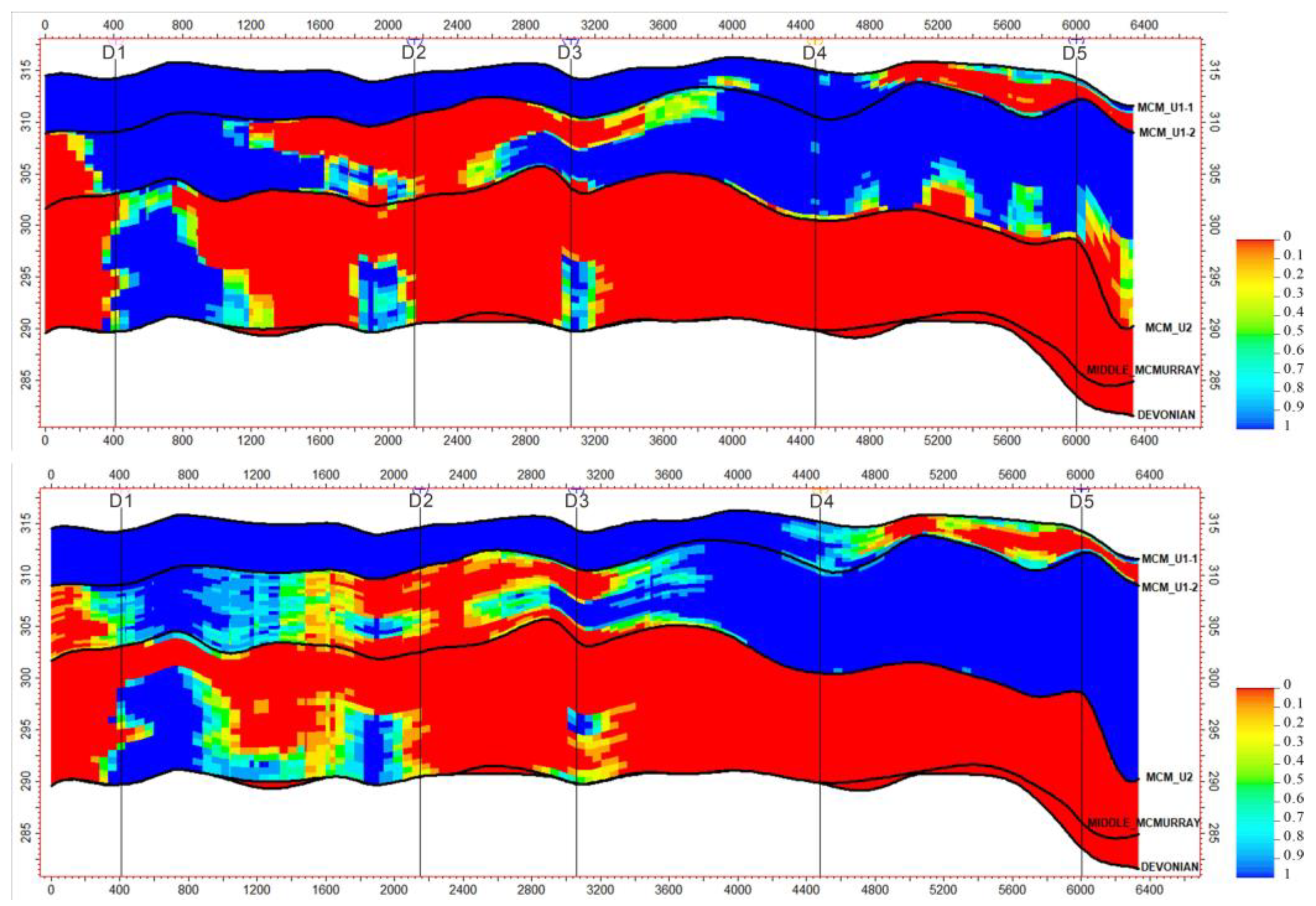
4.3. Model Construction and Analysis

After the input parameters are acquired, the modeling process is executed, and the model is constructed. On the plane, the established facies model has a high similarity with the facies map drawn. The scale of tidal bars varies greatly, and most of them are distributed in continuous sheets and ellipsoids, which are scattered in the sand flat (Figure 12). In the section, the overlapping styles of different sand bodies are well reproduced (Figure 13). The contact relationship and style of sand bodies are consistent with the results of geological dissection. From bottom to top, the number of tidal bars and sand flats increased; the lower part is mainly mixed flat and mud flat, with local point bars. Thick tidal bars and sand flats developed in the upper part. The established model well-reflects the spatial distribution of the architectural elements.
Sequential indication simulation is used to randomly simulate the unknown reservoir space between wells through the known well data and the algorithm under variation function representation. Variation function is the key input parameter of sequential indicator simulation (SIS). The spatial regularity of the sedimentary facies data can be obtained according to variation function analysis of the data points, and then the simulation can be completed. In the sequential indicator simulation, the sedimentary facies data were first coarsened to attach the geological grid of the study area with the sedimentary facies attributes. After that, the variation function analysis of model is implemented for data analysis according to adjusting the main variation, time variation, and nugget value, which can analyze the data in the direction of the vertical content source direction and content source correlation. The experiment of each layer and curve fitting of variational function were calculated as input parameters and guidance for modeling. For comparison, using a traditional sequential indicator method to establish the model, the sand body contact relationship is described in detail in the section (Figure 13). The distribution of sand bodies is different, the randomness is strong, the superior sand bodies are too dominant, and the continuity is strong. Sand bodies with smaller development scales have a smaller distribution range, and some scattered points are more developed. On the plane (Figure 12), the sand bodies in some areas are too continuous, smoothing out many details, and they are scattered in some areas. In addition, there is a great difference between the developed location of the sand body and geological dissection, which leads to a great difference between the established model and the reality.
Furthermore, the prediction results of the two methods are tested based on the seismic interpretation results. The accuracy of the simulated prediction on the section is evaluated by using the matching error between the seismic interpretation and the predicted value. In the direction J = 518, seismic data are used to reveal different sedimentary architecture and distribution patterns (Figure 14a), which are, respectively, predicted by 2D sections and sequential indicator modeling (Figure 14b,c). The architectural elements predicted by the 2D section have good continuity and high similarity with the seismic interpretation results. However, the sequential indicator modeling method is relatively scattered, and the predicted architecture distribution is random, which is very different from the seismic interpretation results. The error statistics of grid-to-grid show that the error of the 2D section prediction method is 25.92%, while sequential indicator modeling is 58.52%. This shows that the prediction result of the 2D section is more accurate. The established model can be used as the basis for subsequent physical property modeling and numerical simulation.

5. Discussion

Reconstructing a 3D model from a 2D section makes good use of the dissection results of 2D architecture and characterizes 3D spatial structure characteristics by fusing the multi-point statistics of different directions, which is a model-guided reservoir prediction method. Therefore, compared with the traditional method of sequential indication modeling (Table 1), all kinds of architectural continuity and superposition styles are more realistic. Compared with the prediction accuracy of the seismic interpretation section, the accuracy of the 2D section reconstruction method is significantly higher than sequential indicator modeling. Considering that the reservoir architecture pattern of the method is from the sections, the distance from the section will affect the accuracy of the model prediction. Based on this consideration, a section (J = 692) is reinterpreted using seismic data in a region far away from the TI and compared with the prediction results of the two methods point-to-point (Figure 15). The result shows that the absolute error is 33.13% based on 2D section modeling. The sequential indicator simulation is 57.25%. From the comparison results, sequential indicator modeling is dependent on the variogram and conditional data, so the error changes little. However, the method based on the 2D section extracts patterns from 2D TIs. If the distance is far from the position of the TIs, the pattern changes greatly, resulting in an increased difficulty of prediction.
To solve the accuracy of the model, it is a natural choice to increase the number of sections and reduce the distance between the estimated point and the section. In this study, two cross-sections are re-added in the area of the thin well pattern (Figure 16), and 10 wells are extracted for cross validation. In order to avoid the risk of a single simulation, a total of 10 simulations are carried out, and then error statistics are carried out to reflect the accuracy of model prediction through the average error. From the statistical results, the method based on the 2D section has high accuracy in reservoir prediction, and the model has little variation. The average error of the tidal bar in cross-validated wells is 8%, and the error range is 0%–35%. The average error in sand flats is 10%, and the error range is 0%–43.6%. The sequential indicator modeling model is highly variable, the average error of the tidal bar is 11.5%, and the error range is 0%–42.2%. The average error is 12.1%, and the range of error is 0%–51.6%.
Increasing the number of sections can improve the accuracy of the model, but this means increasing the workload. In addition, the prediction effect does not increase significantly with numerous sections. Therefore, there is a trade-off between the number of sections used for simulation and accuracy, which needs to be considered in practical applications to obtain the optimal geological model by the most economical method.

6. Conclusions

The oil sand reservoir of the McMurray Formation in Mackay River is a tide-dominated estuary deposit. Nine architectural elements—tidal bar, sand flat, mixed flat, mud flat, salt marsh, tidal channel, point bar, sandy channel filling and salt marsh–can be identified on the core. Influenced by paleo-tectonic structure, paleo-incised geomorphology, and paleo-sea level, different parts of the McMurray Formation have different architecture scales and development patterns. On the section, mud flat, mixed flat, sand flat, and tidal bar are developed from bottom to top. In the lower part, tidal channels and scour filling structures are mostly developed, while in the upper part, mud flat is gradually transformed into sand flat and tidal bar. The high angle continuous lateral accretion can be seen in the sand flat and tidal bar. On the plane, the river deposition from south to north gradually transitions to a tidal estuary, whose geomorphology gradually widens and is filled by tidal flat, tidal bar, and other architectural elements. In the section, the lateral splicing contact among sand bodies is summarized, and four architectural elements’ superposition patterns of SF-TB1-SF, ST-TB1-SF, SF-SF, and SF-MF are summarized.
By scanning the plane section’s architecture of the 2D data template, the superposition pattern and distribution rule of the architecture sand body are extracted. The probability fusion method was used to obtain the multi-point statistical probability of the architectural elements in 3D space, and the elaborate 3D model of the study area was established. The established sedimentary facies model is more similar to the sedimentary facies map drawn by geology, and the tidal bars are distributed in sheets and ellipsoids and scattered in the sand flat. The established model well-reflects the spatial distribution of the sand bodies. The absolute error of reconstruction of the 3D geological model from 2D sections is 33.13%, and the sequential indicator simulation is 57.25%. Therefore, compared with the traditional sequential indication modeling method, it is more successional and realistic. All in all, reconstruction of the 3D geological model from 2D sections is superior to sequential indicator simulation. The accuracy of the developed model is proved by the comparison of grid-to-grid and cross-validation. This study provides a reference for the 3D geological modeling of a tide-dominated estuarine reservoir.

Author Contributions

Conceptualization, Y.Y. and D.Y.; Methodology, Y.Y, J.H. (Jiaxuan Huang) and J.H. (Jixin Huang); software, Y.Y. and W.Z.; validation, J.H. (Jiaxuan Huang), J.H. (Jixin Huang) and W.Z.; formal analysis, Y.Y. and W.Z.; resources, J.H. (Jiaxuan Huang) and J.H. (Jixin Huang); writing—original draft preparation, W.Z.; writing—review and editing, Y.Y., J.H. (Jiaxuan Huang) and J.H. (Jixin Huang); supervision, D.Y.; project administration, J.H. (Jixin Huang) and D.Y. All authors have read and agreed to the published version of the manuscript.

Funding

This research was funded by [the National Natural Science Foundation of China] grant number [42130813, 41872138].

Data Availability Statement

Not applicable.

Acknowledgments

We are very thankful for the hard work of the reviewers and editors.

Conflicts of Interest

We confirm that we have no known competing financial interests or personal relationships that could have appeared to influence the work reported in this paper.

References

  1. Dalrymple, R.W.; Knight, R.J.; Zaitlin, B.A.; Middleton, G.V. Dynamics and facies model of a macrotidal sand-bar complex, Cobequid Bay-Salmon River Estuary (Bay of Fundy). Sedimentology 1990, 37, 577–612. [Google Scholar] [CrossRef]
  2. Bostock, H.C.; Brooke, B.P.; Ryan, D.A.; Hancock, G.; Pietsch, T.; Packett, R.; Harle, K. Holocene and modern sediment storage in the subtropical macrotidal Fitzroy River estuary, Southeast Queensland, Australia. Sediment. Geol. 2007, 201, 321–340. [Google Scholar] [CrossRef]
  3. Ryan, D.A.; Brooke, B.P.; Bostock, H.C.; Radke, L.C.; Siwabessy, P.J.; Margvelashvili, N.; Skene, D. Bedload sediment transport dynamics in a macrotidal embayment, and implications for export to the southern Great Barrier Reef shelf. Mar. Geol. 2007, 240, 197–215. [Google Scholar] [CrossRef]
  4. Liu, C.; Zhang, Q.; Xie, Y.; Qiao, L.; Sun, J.; Mei, X. Sequence Stratigraphic Framework and Development Model of the Cretaceous in Northeast Block, Oriente Basin, Ecuador. Acta Sedimentol. Sin. 2014, 32, 1123–1131. [Google Scholar] [CrossRef]
  5. Abdelwahhab, M.A.; Radwan, A.A.; Mahmoud, H.; Mansour, A. Geophysical 3D-static reservoir and basin modeling of a Jurassic estuarine system (JG-Oilfield, Abu Gharadig basin, Egypt). J. Southeast Asian Earth Sci. 2021, 225, 105067. [Google Scholar] [CrossRef]
  6. Zhou, H.; Huang, J.; Feng, W.; Liu, S.; Yin, Y. Analysis on formation factors and development characteristics of sand bar in tide-dominated estuaries—A case study based on Qiantang River. Geol. Rev. 2020, 66, 101–112. [Google Scholar] [CrossRef]
  7. Yang, B.; Dalrymple, R.W.; Gingras, M.K.; Chun, S.; Lee, H. Up-Estuary Variation of Sedimentary Facies and Ichnocoenoses in an Open-Mouthed, Macrotidal, Mixed-Energy Estuary, Gomso Bay, Korea. J. Sediment. Res. 2007, 77, 757–771. [Google Scholar] [CrossRef]
  8. Ji, Z.-G.; Hu, G.; Shen, J.; Wan, Y. Three-dimensional modeling of hydrodynamic processes in the St. Lucie Estuary. Estuar. Coast. Shelf Sci. 2007, 73, 188–200. [Google Scholar] [CrossRef]
  9. Dalrymple, R.W.; Choi, K. Morphologic and facies trends through the fluvial–marine transition in tide-dominated depositional systems: A schematic framework for environmental and sequence-stratigraphic interpretation. Earth-Sci. Rev. 2007, 81, 135–174. [Google Scholar] [CrossRef]
  10. Cheng, L.; Yin, Y.; Wang, H.; Feng, W.; Wang, L.; Liu, Z.; Wang, P.; Liu, J. Analysis of the internal architectural elements of tidal-influenced meandering fluvial deposits using well logging and seismic data: The study of the Athabasca Oil Sands, Alberta, Canada. Interpretation 2020, 8, SM103–SM114. [Google Scholar] [CrossRef]
  11. Tang, M.; Zhang, K.; Huang, J.; Lu, S. Facies and the architecture of estuarine tidal bar in the lower Cretaceous Mcmurray For-mation, Central Athabasca Oil Sands, Alberta, Canada. Energies 2019, 12, 1769. [Google Scholar] [CrossRef] [Green Version]
  12. Tang, M.; Lu, S.; Zhang, K.; Yin, X.; Ma, H.; Shi, X.; Liu, X.; Chu, C. A three dimensional high-resolution reservoir model of Napo Formation in Oriente Basin, Ecuador, integrating sediment dynamic simulation and geostatistics. Mar. Pet. Geol. 2019, 110, 240–253. [Google Scholar] [CrossRef]
  13. Tang, J.F.; Tang, M.M.; Lu, S.F.; Liu, X.P.; Zhang, K.X.; Hua, H.T.; Han, D. Three-Dimensional Modeling of Estuary Reservoir Based on Coupling Sedimentary Dynamics Simulation and Multipoint Geostatistics Method[J/OL]. Earth Science. Available online: http://kns.cnki.net/kcms/detail/42.1874.P.20220621.1503.016.html (accessed on 7 October 2022).
  14. Okabe, H.; Blunt, M.J. Prediction of permeability for porous media reconstructed using multiple-point statistics. Phys. Rev. E 2004, 70, 066135. [Google Scholar] [CrossRef] [PubMed] [Green Version]
  15. Okabe, H.; Blunt, M.J. Pore space reconstruction using multiple-point statistics. J. Pet. Sci. Eng. 2005, 46, 121–137. [Google Scholar] [CrossRef]
  16. Comunian, A.; Renard, P.; Straubhaar, J. 3D multiple-point statistics simulation using 2D training images. Comput. Geosci. 2011, 40, 49–65. [Google Scholar] [CrossRef] [Green Version]
  17. Takamura, K. Microscopic structure of athabasca oil sand. Can. J. Chem. Eng. 1982, 60, 538–545. [Google Scholar] [CrossRef]
  18. Carrigy, M.A. Geology of the McMurray Formation: General Geology of the McMurray AreaResearch Council of Alberta. Geological Division. 1959, 1, 130. [Google Scholar]
  19. Hein, F.J.; Cotterill, D.K. The Athabasca Oil Sands—A Regional Geological Perspective, Fort McMurray Area, Alberta, Canada. Nonrenewable Resour. 2006, 15, 85–102. [Google Scholar] [CrossRef]
  20. Barton, M.D.; Seibel, C. The architecture and variability of valley-fill deposits within the Cretaceous McMurray Formation, Shell Albian Sands Lease, northeast Alberta. Bull. Can. Pet. Geol. 2016, 64, 166–198. [Google Scholar] [CrossRef]
  21. Phillips, J. Sedimentology, Ichnology, and Development of a Sub-Regional Depositional and Stratigraphic Framework for the McMurray-Wabiskaw Succession in the MacKay River Area, Northeastern Alberta. Master’s Thesis, University of Alberta, Edmonton, AB, Canada, 2011. [Google Scholar] [CrossRef]
  22. Mutti, E. Turbidite Systems and Their Relations to Depositional Sequences. In Provenance of arenites; Springer: Dordrecht, The Netherlands, 1985; pp. 65–93. [Google Scholar] [CrossRef]
  23. Dalrymple, R.W.; Zaitlin, B.A.; Boyd, R. Estuarine facies models; conceptual basis and stratigraphic implications. J. Sediment. Res. 1992, 62, 1130–1146. [Google Scholar] [CrossRef]
  24. Qi, Y. Research on Estuarine Facies Models. Bull. Geol. Sci. Technol. 1999, 1, 46–50. [Google Scholar]
  25. Zhang, T.; Lu, T.; Li, D. A method of reconstruction of porous media using a two-dimensional image and multiple-point statis-tics. J. Univ. Sci. Technol. China 2010, 40, 271–277. [Google Scholar]
  26. Zheng, T.; Hou, W.; He, S. An MPS-Based Simulation Algorithm for 3D Geological Structure with 2D Cross-Sections. J. Jilin Univ. 2019, 49, 1496–1506. [Google Scholar] [CrossRef]
  27. Hou, W.; Liu, H.; Zheng, T.; Shen, W.; Xiao, F. Hierarchical MPS-Based Three-Dimensional Geological Structure Reconstruction with Two-Dimensional Image(s). J. Earth Sci. 2021, 32, 455–467. [Google Scholar] [CrossRef]
  28. Okabe, H.; Blunt, M. Pore space reconstruction of vuggy carbonates using microtomography and multiple-point statistics. Water Resour. Res. 2007, 43. [Google Scholar] [CrossRef]
  29. Chen, Q.; Mariethoz, G.; Liu, G.; Comunian, A.; Ma, X. Locality-based 3-D multiple-point statistics reconstruction using 2-D geological cross sections. Hydrol. Earth Syst. Sci. 2018, 22, 6547–6566. [Google Scholar] [CrossRef] [Green Version]
  30. Wang, L.; Yin, Y.; Wang, H.; Zhang, C.; Feng, W.; Liu, Z.; Wang, P.; Cheng, L.; Liu, J. A method of reconstructing 3D model from 2D geological cross-section based on self-adaptive spatial sampling: A case study of Cretaceous McMurray reservoirs in a block of Canada. Pet. Explor. Dev. 2021, 48, 407–420. [Google Scholar] [CrossRef]
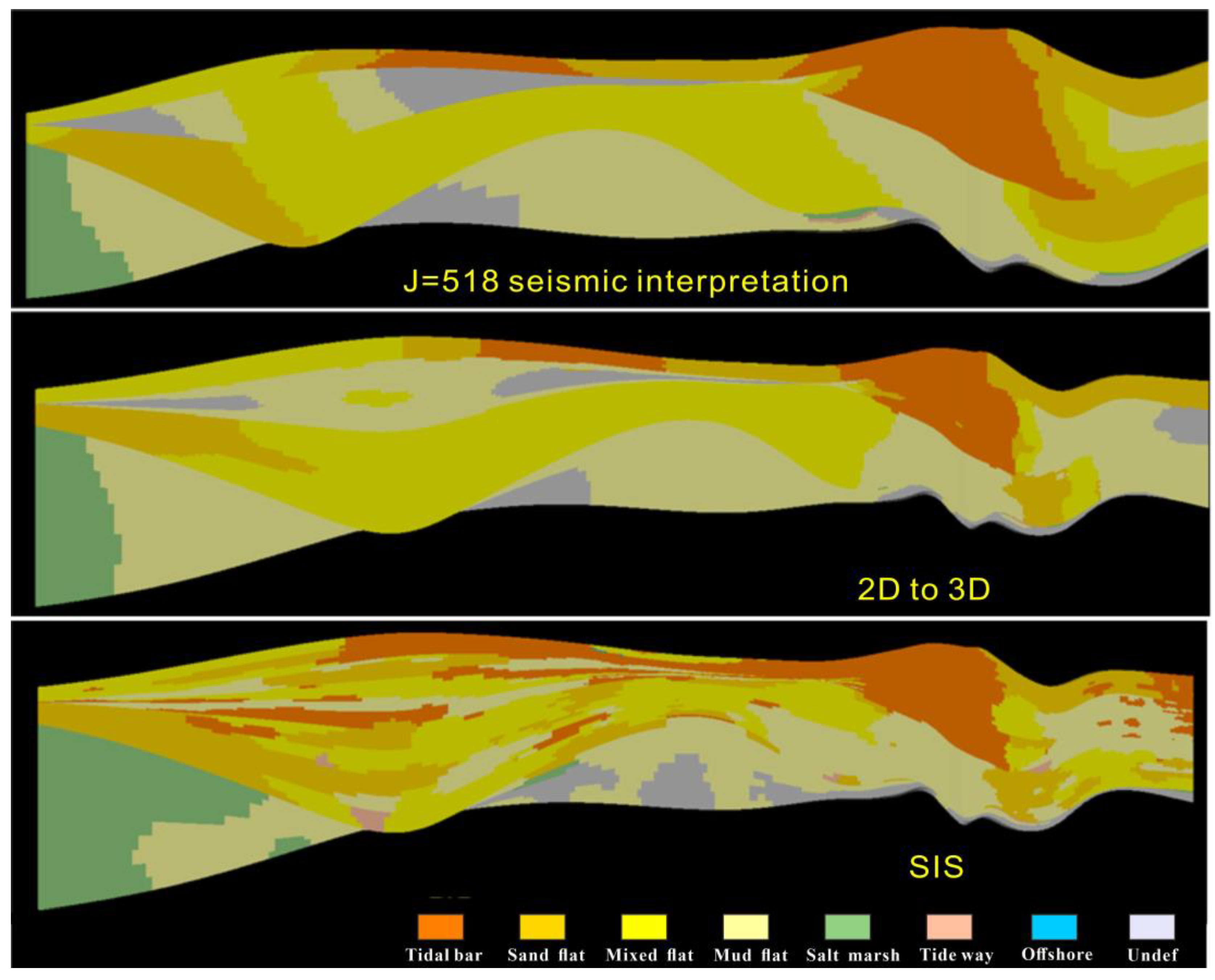
Figure 1. Structural diagram of the study area. DD′ and EE′ are the section location shown in Figure 10. FF′ is the 2D seismic section shown in Figure 9.
Minerals 12 01420 g001
Figure 2. Architecture analysis of 2D seismic slice. The GR curve is on the left, the lithofacies association is in the middle, and the RESS curve is on the right.
Minerals 12 01420 g002
Figure 3. Core data of FA1–FA9 lithofacies associations. (a) Core data of sandy channel filling; (be) Core data of point bar; (fh) Core data of salt marshes; (i,j) Core data of point bar in tidal channels; (k) Core data of mudflat; (l) Core data of mixed flat; (m) Core data of sand flat; (nq) Core data of tidal bar; (r) Core data of offshore.
Minerals 12 01420 g003
Figure 4. The location of sections in Figure 5, Figure 6 and Figure 7 (A1–A6 is the location of cross-section 1, B1–B7 is the location of cross-section 2, and C1–C7 is the location of longitudinal section.). And it’s also the planar map of architectural elements in U1-1. The blue dashed lines represent different periods of accretions, the complex of the tidal bar in the incised valley is lateral accretion, and the others are forward accretions.
Minerals 12 01420 g004
Figure 5. (a) Two-dimensional seismic section interpretation of cross-section 1. The GR curve is on the left, and the RESS curve is on the right. (b) Architectural elements analysis of cross-section 1. MCMR is an abbreviation for McMurray. (The section location is shown in Figure 4).
Minerals 12 01420 g005
Figure 6. Architectural elements analysis of cross-section 2. (The section location is shown in Figure 4).
Minerals 12 01420 g006
Figure 7. (a) Two-dimensional seismic section interpretation of the longitudinal section. The Gr curve is on the right, and the RESS curve is on the left. (b) Architectural elements analysis in the longitudinal section. (The section location is shown in Figure 4).
Minerals 12 01420 g007
Figure 8. The superposition patterns of architectural elements. TB is tidal bar, SF is sand flat, and MF is mixed flat.
Minerals 12 01420 g008
Figure 9. (a) Middle McMurray was deposited in contact with carbonate basement; (b) Upper McMurray was deposited in contact with carbonate basement; (c) 2D seismic section in cross-section. (The section location FF’ is shown in Figure 1).
Minerals 12 01420 g009
Figure 10. Incision and fill pattern of the McMurray Formation. (The section location is shown in Figure 1).
Minerals 12 01420 g010
Figure 11. Two-dimensional TIs obtained based on geological architecture dissection.
Minerals 12 01420 g011
Figure 12. Comparison of modeling results.
Minerals 12 01420 g012
Figure 13. Comparison test of modeling results.
Minerals 12 01420 g013
Figure 14. Comparison of seismic interpretation section and prediction results. (a) The seismic interpretation section in the direction of J = 629; (b) the prediction result of 2D to 3D. (c) the prediction result of SIS.
Minerals 12 01420 g014
Figure 15. Comparison of seismic interpretation section and prediction results.
Minerals 12 01420 g015
Figure 16. Comparison of E-type results of drained test wells.
Minerals 12 01420 g016
Table 1. Comparison of two methods (2D to 3D and SIS).
2D to 3DSIS
Method2D training image acquisition mode, condition points as constraints.Conditional data are used as constraints, and the curve fitting of variation function is used as input parameter constraints.
Simulation error All33.13%All57.25%
Tidal bar8%Tidal bar11.5%
Sand flat10%Sand flat12.1%
Error rangeTidal bar0%–35%Tidal bar0%–42.2%
Sand flat0%–43.6%Sand flat0%–51.6%
AdvantagesThe reservoir architecture and morphology can be well captured from TIs so that the three-dimensional reservoir structure and morphology can be well reproduced.Make good use of the existing geological information. Quick simulation.
DisadvantagesSimulation efficiency is low because of workload.It cannot well-reflect the reservoir morphology and configuration superimposition style.
Publisher’s Note: MDPI stays neutral with regard to jurisdictional claims in published maps and institutional affiliations.

