

Grid-Characteristic Method on Overlapping Curvilinear Meshes for Modeling Elastic Waves Scattering on Geological Fractures

1
Moscow Institute of Physics and Technology, 9 Institutskiy Lane, Dolgoprudny 141701, Russia
2
Scientific Research Institute for System Analysis of the Russian Academy of Sciences, Moscow 117218, Russia
*
Author to whom correspondence should be addressed.
Minerals 2022, 12(12), 1597; https://doi.org/10.3390/min12121597
Submission received: 2 November 2022
/
Revised: 26 November 2022
/
Accepted: 10 December 2022
/
Published: 12 December 2022
(This article belongs to the Special Issue Feature Papers in Mineral Exploration Methods and Applications 2022)
Abstract
:Interest in computational methods for calculating wave scattering from fractured geological clusters is due to their application in processing and interpreting the data obtained during seismic prospecting of hydrocarbon and other mineral deposits. In real calculations, numerical methods on structured, regular (Cartesian) computational grids are used to conserve computational resources though these methods do not correctly model the scattering of elastic waves from fractures that are not co-directed to the coordinate axes. The use of computational methods on other types of grids requires an increase in computational resources, which is unacceptable for the subsequent solution of inverse problems. This article is devoted to a possible solution to this problem. We suggest a novel modification of a computational grid-characteristic method on overlapping curvilinear grids. In the proposed approach, a small overlapping curvilinear grid is placed around a fracture that smoothly merges into the surrounding Cartesian background mesh, which helps to avoid interpolation between the background and overlapping meshes. This work presents the results of testing this method, which showed its high accuracy. The disadvantages of the developed method include the limited types of fractured clusters for which this method can be applied since the overlapping meshes should not intersect. However, clusters of subvertical fractures are usually found in nature; therefore, the developed method is applicable in most cases.
1. Introduction
A large number of mineral deposits is associated with the presence of fluid-saturated fractures. This is often associated with volcanic zones [1]. Fluid-saturated fractured inclusions can be used to analyze mineral deposits [2]. Interpretation of seismic data obtained from mineral deposits requires the development of sufficiently effective methods to account for micro and macro fractures. Fault zones and fractured zones are quite common in the vicinity of open deposits. Seismic survey methods are used to explore ore deposits [3,4], so developing more accurate methods for seismic modeling and constructing mathematical models of geological environments is important for this area. However, multiple solutions to the corresponding direct problems are required to perform a full-wave inversion. This makes it necessary for scientists to develop computational methods for solving direct problems of the elastic wave equation that can describe the real geometry of a fractured cluster and conserve computing resources at the same time.
The accuracy of modeling the scattering of elastic waves on a fracture certainly depends on the mathematical model used. The Schoenberg linear slip model [5] (LSM) has proven to be consistent with practice [6,7] and is the most commonly used. We have also used it in this work. An anisotropic model [8] of an elastic medium is usually used and is acceptable at sufficiently long wavelengths. This mathematical model makes it possible to reduce the number of computational resources, but not all types of waves scattered by fractures in nature are taken into account. Using the explicit method [9,10] is more accurate, and we use it in this work.
Fracture models differ in the computational grids used to describe the fracture itself. It is possible to distinguish such approaches as the use of Cartesian grids inside the fracture, codirectional with the coordinate axes [11,12], Cartesian grids and the model of infinitely thin fractures, codirectional [13,14,15,16] and not codirectional with the coordinate axes [17]. The approach proposed in [17] requires small coordinate steps to describe the fracture shape and correctly calculate the scattered waves. It can be concluded that the use of a Cartesian grid imposes restrictions on the orientation of fractures, which, in turn, will not make it possible to determine the important parameters of a fractured cluster, such as fracture orientation, fracture orientation spread, etc., or requires significant discretization to achieve sufficient calculation accuracy.
The methods for modeling incident and scattered elastic waves are divided into finite-difference methods [13,18,19,20,21] (which include, for example, the grid-characteristic method [12,16,17,22,23], and staggered-grid method [24,25,26,27]), finite element methods [28,29,30] (which include, for example, the discontinuous Galerkin method [31,32] and the method of spectral elements [33,34,35,36]). In addition, other methods, e.g., discrete particle schemes might be used [37].
Moreover, computational methods for modeling wave propagation in fractured geological media differ in the types of computational meshes used. These meshes can be Cartesian [13,17,23], curvilinear [28,37,38], unstructured triangular [9,23,28,39,40,41,42], tetrahedral [10,23,43], and quadrangular [40]. It can be concluded that only the use of Cartesian grids provides sufficient computational speed for solving real inverse problems of geophysics [44].
In [22], we proposed a grid-characteristic method on Chimera meshes. Chimera meshes [45,46] (also known as adaptive [47], overset [48], composite overlapping [49,50] meshes, or chimera method [51]) were used for the first time to solve problems of hydrodynamics [52,53,54,55]. Currently, they are used for other problems, for example, to solve the Poisson problem [56]. When using chimera meshes, the advantage is the Jacobian unit of the coordinate transformation in the grid surrounding the fracture due to the chimera mesh is Cartesian. Therefore, the method ensures the time step does not decrease. The disadvantage here is the need to interpolate the solution from the grid surrounding the fracture into the background computational grid. When using overlapping curvilinear meshes, which we propose in this work, the advantage is the absence of interpolation since the outside nodes of the curvilinear mesh coincide with the nodes of the background mesh, and the disadvantage is not the unit Jacobian of the coordinate transformation. In this work, we carry out the same tests as in work [22] to compare both approaches.
Curvilinear computational grids have been used for a long time in various fields. Let us consider applying computational curvilinear grids to the solution of elastic and acoustic wave equations in recent years. The method of pseudo-spectral elements to calculate the SH waves in a 2D case was used in [36]. The structured curvilinear meshes, also known as body-fitted and boundary-conforming meshes, were used to take into account the Earth’s topography with the help of finite differences on modified staggered grids [27]. An efficient and accurate numerical algorithm for the simulation of borehole acoustic experiments using curvilinear meshes is presented in [38]. This type of grid is also used for accurate modeling of a free boundary of complex shapes [57].
This paper is organized as follows. The mathematical formulation of the problem and the features of the proposed modification of the numerical method are presented in Section 2. The features of the used overlapping curvilinear grids are discussed in Section 3. Section 4 discusses the testing of the proposed numerical method, and Section 5 presents the results of calculations of elastic wave scattering on geological models of fractured media of various complexity. The conclusions are presented in Section 6.
2. Computational Method
This section is devoted to the solved system of equations and the description of the proposed modification of the computational method. The features of constructing curvilinear computational grids surrounding the fractures in the geological media are considered in the next section.
2.1. Mathematical Statement
The conversion from the LMS model [5] of fractured media to the following initial-boundary value problem for the elastic wave equation is considered in detail in our previous work [22].
Here and further in the text, , represent the unknowns of the velocity and symmetric Cauchy stress tensor of the second rank, denotes the density, , represent the speeds of the pressure (P-) and shear (S-) elastic waves, respectively; means the unit tensor of the second rank; denotes the tensor product of vectors, ; , are the coordinate vector in the integration domain and the time, respectively; denotes coordinates of infinity thin fracture ; and denotes the unit vector normal to the fracture in the point .
Note that when using this type of notation, the presented initial-boundary value problem has the same form in both three-dimensional and two-dimensional cases.
Different types of sources were used, e.g., a plane P-wave as an initial condition or point sources and zero initial conditions. The source type is described in Section 5 for each specific problem being solved.
2.2. Grid-Characteristic Method on Structured Curvilinear Meshes
We introduce the coordinate transformation . The structured curvilinear grid in the introduced coordinate system will turn into a Cartesian grid with a unit step in coordinates. Herewith, we know the positions of the nodes of the structured curvilinear grid in the original coordinate system.
There is no need to look for a coordinated transformation in the analytical form. We numerically calculate all quantities necessary for subsequent calculations. That is, for each node of the structured curvilinear grid and each direction , we introduce the following vector :
Furthermore, we introduce vectors as being perpendicular to the vectors . Now, we can consider a set of symmetric tensors of the second rank for each pair of vectors and :
Here, .
Further, for each point of the curvilinear grid, the formulae from our previous work [22] can be applied to calculate unknown values for each of the directions.
2.3. Computational Algorithm
In the proposed modification of the grid-characteristic method using overlapping curvilinear grids, we use the following computational algorithm for every time step .
- 1.
- Values from the background grid are copied in two layers of nodes placed along the vertical boundaries of the curvilinear grids and surrounding fractures. Section 4 describes in detail the features of constructing these curvilinear grids in the proposed modification of the computational method, which makes it possible to carry out this copying and, at the same time, obtain high accuracy of calculations.
- 2.
- Calculations are carried out in the direction OX in the background grid by the grid-characteristic method on Cartesian grids, described in [22].
- 3.
- Calculations are also performed for the OX direction in each curvilinear meshes surrounding the fractures using the grid-characteristic method on structured curvilinear meshes described in the next section.
- 4.
- Values from two layers of nodes of curvilinear grids placed along the vertical boundaries are copied in the congruent position nodes of the background grid.
Then, all these four steps are performed for the direction OY and the horizontal boundaries.
This algorithm can be easily generalized to the three-dimensional case. The boundaries will be replaced herewith by the corresponding planes perpendicular to the directions under consideration.
Below we provide a pseudocode showing the sequence of implementation of the various stages of the algorithm in the software. When implemented, it is necessary to carry out the sequence of interpolation correctly to the boundary nodes of overlapping curvilinear meshes with fractures and to the nodes of the background mesh from the meshes with fractures within the time integration cycle. The sequence is displayed in pseudocode.
3. Features of Curvilinear Computational Meshes
A curvilinear computational mesh is built from the following principles. The outer two rows of curved mesh cells strictly coincide with the background mesh cells to not use interpolation but copy from these two rows to the background mesh (Figure 1A, red (black) nodes) and back to the ghost nodes of the curvilinear mesh from the background mesh (Figure 1A, blue (grey) nodes). Next, a third-order polynomial is constructed to ensure the continuity of the first derivative on the line marked in color and thickness in Figure 1B. The areas of the third-order polynomial are marked in red lines of middle thickness, and the crack area is shown in green lines with maximal thickness in the center. The blue lines with maximal thickness near the edges ensure an exact match with the background grid.
| Pseudocode |
|
Next, for the sake of simplicity, consider the mesh for a fracture with an angle less than the horizontal (Figure 1B). The number of cells around the crack is chosen automatically so that the vertical distance between the cells does not exceed a certain (Figure 1B and Figure 2A). The number of nodes along the horizontal is chosen so that the inclination angle between the adjacent cells along the vertical edge does not exceed a fixed angle (Figure 1B and Figure 3). The vertical step in the grid changes smoothly according to the following function:
Figure 2A demonstrates at what angles of inclination of the fracture it is suitable to use , and at what angles it is suitable to use . The Courant number in the background mesh required for the stability of the method on a curvilinear mesh is close to the ratio (Figure 2B) for , and is the optimal parameter of the curvilinear mesh construction. The suitability of is also confirmed by the graphs in Figure 3 since, for this value the size of the curvilinear mesh is also optimal.
Let us provide some examples of computational structured curvilinear meshes around the fractures for the different fracture’s inclination angles (Figure 4). These fractures are colored red. There are 10 nodes of the Cartesian background grid per the fracture for all inclination angles. One can see the dependence of the number of nodes on the fracture’s inclination angle.
4. Testing
In this section, we study the quality of calculation of the types of waves reflected from a crack depending on the angle between the crack and the OX axis. To do this, we compare synthetic seismograms obtained from receivers located on a circle around the center of the fracture (Figure 5A), calculated using the proposed modification of the grid-characteristic method on overlapping curvilinear meshes and calculated using the grid-characteristic method on Cartesian grids. The Ricker wavelet point source with a frequency of 20 Hz was placed near the first receiver (Figure 5A). To model the fracture’s inclination and use a fracture co-directed to the OX axis, we rotate the circles on which the source and receiver lie in accordance with Figure 5B. The angle α is the angle between the fracture and the horizontal axis OX for Figure 5A and the inclination angle for Figure 5B, respectively.
We used the coordinate step of 2 m, the fracture length of 100 m, the P-wave speed of 1000 m/s, the S-wave speed of 600 m/s, and the density of 1000 kg/m3. The maximum time step in all calculations was equal to 0.8 ms. Note that the time step depends on the angle α due to stability conditions. This issue was discussed in Section 3.
The dependence of the relative errors on α is shown in Figure 6. We have used the following formulae to calculate relative errors:
In (11) and (12), , denote the velocity field components obtained using the proposed method in the original coordinate system; , represent the velocity field components obtained without an overlapping curvilinear mesh in the coordinate system rotated on angle α. In (11) and (12) and further in the text, denotes the number of receivers that equals 36; NT denotes the number of time steps that depends on the time step in considered calculation with considered α. depends on α due to the constant total time was used for each α, and different time steps were used.
The dependence of the relative errors of the anomalous velocity on the angle α is shown in Figure 7. To calculate the relative errors of the anomalous field, we used the following formulae:
In (13) and (14), , are the anomalous velocity field components calculated using the proposed method of the original coordinate system; , are the anomalous velocity field components of the calculated without an overlapping curvilinear mesh in the respectively rotated coordinate system.
The examples of velocity field snapshots and seismograms for the angle α of 30° are shown in Figure 8, Figure 9 and Figure 10.
The testing performed demonstrates the high accuracy of the proposed numerical method.
We specifically used such a discretization from 17 to 25 points (in dependence on the inclination between the wavefront and the coordinate axis) of the background computational mesh are used to treat the P-waves, and from 10 to 15 points are used to treat the S-waves. This allows for a more representative comparison of the proposed method with available alternatives, including the one presented in [22].
To clarify how specifically Figure 8, Figure 9, Figure 10 and Figure 11 differ, we present a series of one-dimensional plots in Figure 12, Figure 13, Figure 14, Figure 15, Figure 16, Figure 17, Figure 18, Figure 19 and Figure 20.
The data on the plots in Figure 12, Figure 13, Figure 14, Figure 15, Figure 16, Figure 17, Figure 18, Figure 19 and Figure 20 are registered by the receivers marked by red color in Figure 8 and correspond to vertical lines on the seismograms in Figure 9, Figure 10 and Figure 11.
By the X- and Y-components of velocity, we mean the components in the non-rotated coordinate system introduced in Figure 5A. Thus, to obtain the plotted data, the original data for the problem «without overlapping curvilinear mesh» were transformed by rotating by the appropriate angle of 30°.
The choice of receiver numbers for plotting is due to the following factors. Figure 12, Figure 13 and Figure 14 (Receiver #4), Figure 18, Figure 19 and Figure 20 (Receiver #19) correspond to two converted PS waves, respectively. Figure 15, Figure 16, Figure 17, Figure 18 and Figure 19 (Receiver #7) correspond to PP-wave reflected from the fracture.
5. Results of Numerical Experiments
In this section, we present the results of the test calculations for the different geological models of fractured media of varying complexity. We took similar geological models as in [22] to compare the results obtained.
5.1. Example #1
A set of fractures with arbitrary length, location, and orientation (Figure 21, Figure 22, Figure 23 and Figure 24) is considered in this section. This model is based on the one given in [39]. The initial conditions of a plane elastic P-wave (Figure 21 and Figure 22) or S-wave (Figure 23 and Figure 24) with a wavelet length being equal to 50 m, half-sine wave profile (effective frequency of 50 Hz, real frequency of 25 Hz), and a unit amplitude was applied. We used a coordinate step of 1 m and a time step of 0.16 ms. In [22], we used a time step of 0.3 ms in a similar test. The P-wave speed of 3000 m/s, the S-wave speed of 2000 m/s, and the density of 2500 kg/m3 were used in this section and Section 5.2 and Section 5.3.
The presented results show a more significant dispersion of the transmitted S-waves compared to the P-waves. It can also be seen that the developed method managed well with modeling the passage of plane waves through a cluster of multidirectional fractures of different sizes. However, the model from [39] had to be modified so that the overlapping curvilinear meshes surrounding the fractures did not intersect with each other.
5.2. Example #2
The model from [9] is discussed in this section. We used a point source marked by the red dot in Figure 25A with a source function of Ricker wavelet; a peak frequency equals 30 Hz. The coordinate step of 2 m, and the time of 0.2 ms were used. In [22], in a similar test, we used a time step of 0.6 ms for the same coordinate step in the background mesh. In [9] in the similar test, the time step was equal to 1 ms for triangular mesh with an edge length varying around 4 m. Figure 25 and Figure 26. show the used model and snapshots of the calculated elastic wave field at the time moment of 0.555 s.
5.3. Example #3
This section discusses the model from [9]. We model wave propagation in the fractured zone, in which there are 101 fractures rotated at 30° with a horizontal distance of 42 m between them. We used the same point source as in the previous Section 5.2, the coordinate step of 2 m, and the time step of 0.16 ms. In [22], in a similar test, we used a time step of 0.6 ms for the same coordinate step in the background mesh. In [9], in the similar test, the time step was equal to 1 ms for triangular mesh with an edge length varying around 4 m. Figure 27 and Figure 28. show the used model and snapshots of the calculated elastic wave field snapshots at the time moment of 0.86 s.
5.4. Example #4
In this section, we discuss the geological model based on one from [39]. In our model, the fractures are subvertical. We used the coordinate step of 0.78125 m, and the time step of 50 ; they are the same as in [22]. Figure 29 and Figure 30 show the model and the calculated elastic wave field snapshots at a time moment of 0.25 s.
One can conclude that the proposed grid-characteristic method using overlapping curvilinear meshes is limited by the size of the curvilinear mesh surrounding the fracture and is well suited for describing only a certain type of fracture cluster, e.g., the clusters of subvertical fractures.
5.5. Example #5
In this section, we consider the model from [4]. The study aims to show how fractures in the geological media affect wave fields and seismograms arising from metal ore bodies seismic exploration. To do this, we placed two types of fractured zones above and next to the metal ore body. Accordingly, we obtain three calculations: «without fractured zone» (Figure 31A), the fractured zone above the metal ore body («fractured zone #1», Figure 32A), and the fractured zone next to the metal ore body («fractured zone #2», Figure 32B). Below, in Figure 33, Figure 34 and Figure 35, snapshots of wave fields and seismograms are presented.
All scales of fields used in this section are introduced in Figure 31B–D.
The source was a Ricker wavelet with a frequency of 30 Hz, marked by the red dot in Figure 31 and Figure 32A. The space step was 1.6 m. Due to the different geometry of the fractures in the problems «fractured zone #1» and «fractured zone #2», the time steps were different in accordance with the stability conditions. Accordingly, we obtain time steps of 0.2 ms, 0.0779 ms, and 0.07 ms for the problems «without fractured zone», «fractured zone #1», and «fractured zone #2», respectively. Thus, the total time is also slightly different, 1 s, 1.0127 s, 0.98 s, respectively.
For clarity, we have chosen time points 0.275 s and 0.51 s (exact values are given for the problem «without fractured zone») to compare the wave fields. The moment of 0.275 s well reflects the shielding process («fractured zone #1»), and the dynamics of shielding evolution are visible at the time of 0.51 s. For comparison, at 0.275 s («fractured zone #2»), there is practically no shielding since, for this fractured zone and the source position, the re-reflection process begins around the time of 0.51 s.
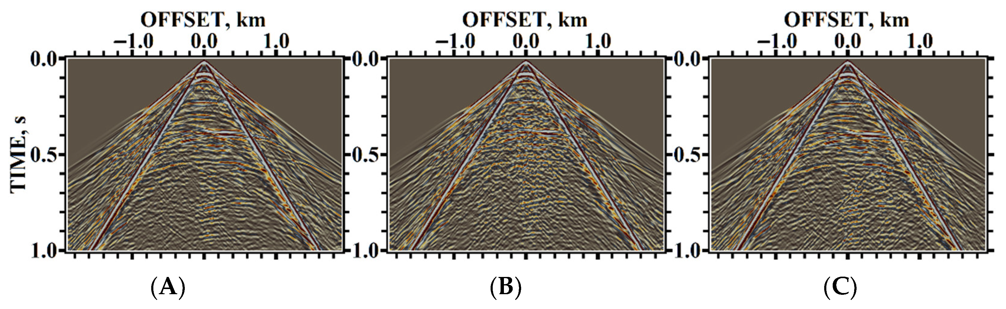
Figure 33, Figure 34 and Figure 35 show how the shielding process is proceeding. The synthetic seismograms demonstrate visible layers in Figure 36A, Figure 37A and Figure 38A and various shielding options in Figure 36B, Figure 37B and Figure 38B, and Figure 36C, Figure 37C and Figure 38C, respectively.
It can be seen that when the fractured zone is located above the metal ore body, the fractured zone has significant shielding properties. While the location of the fractured zone next to the metal ore body, in the case of positioning the source strictly above the metal ore body, although the fractured zone does not provide a significant shielding effect, it also contributes to wave fields and seismograms.
The performed studies show the importance of correct treatment of the scattering of seismic waves on fractured zones for more accurate and precise seismic exploration of minerals.
6. Conclusions
In this work, we proposed a novel modification of the numerical grid-characteristic method using overlapping curvilinear meshes. The proposed approach makes it possible to use a Cartesian background computational mesh in the entire integration domain to accurately simulate the scattering of elastic waves on fractures, which are not codirectional to the coordinate axes, and to avoid interpolation between the overlapping mesh and the background mesh.
The disadvantage of the developed method is that it is not suitable for all configurations of fracture clusters since overlapping meshes must not intersect. However, in nature, most of the fractured zones are characterized by the sub-vertical position of the fractures; therefore, the developed method is applicable in practice.
In contrast to the approach proposed by us in [22], the computational method from this work has a higher accuracy in calculating scattered waves for different fracture orientations. However, the set of geological models to which the method on the overlapping curvilinear mesh is applicable is more limited compared to the use of Chimera meshes. It can also be noted that using curvilinear meshes in the case of fracture’s inclination angles close to 45° requires a significant reduction in the time step in accordance with the stability condition.
Author Contributions
Conceptualization, N.I.K. and A.F.; Methodology, N.I.K. and A.F.; Software, N.I.K., A.F. and V.F.; Validation, A.F. and V.F.; Formal analysis, A.F.; Resources, V.F.; Data curation, N.I.K. and A.F.; Writing—original draft, A.F.; Writing—review & editing, N.I.K.; Visualization, A.F.; Supervision, N.I.K.; Project administration, N.I.K. and A.F. All authors have read and agreed to the published version of the manuscript.
Funding
This work was conducted with the financial support of the Russian Science Foundation (project No. 20-71-10028).
Acknowledgments
This work has been carried out using computing resources of the federal collective usage center Complex for Simulation and Data Processing for Mega-science Facilities at NRC “Kurchatov Institute”, http://ckp.nrcki.ru/.
Conflicts of Interest
The authors declare no conflict of interest.
References
- Feng, M.; Liu, T.; Lin, T.; Liu, X.; Li, N.; Xi, A. Fracture fillings and implication of fluid activities in volcanic rocks: Dixi Area in Kelameili Gas Field, Junggar Basin, Northwestern China. Minerals 2019, 9, 154. [Google Scholar] [CrossRef] [Green Version]
- Parry, W.T. Fault-fluid compositions from fluid-inclusion observations and solubilities of fracture-sealing minerals. Tectonophysics 1998, 290, 1–26. [Google Scholar] [CrossRef]
- Zheng, Y.; Liu, Y.; Xu, T.; Li, Z. Elastic Correlative Least-Squares Reverse Time Migration Based on Wave Mode Decomposition. Processes 2022, 10, 288. [Google Scholar] [CrossRef]
- Zhang, F.; Zhang, P.; Xu, Z.; Gong, X.; Han, L. Multisource Seismic Full Waveform Inversion of Metal Ore Bodies. Minerals 2021, 12, 4. [Google Scholar] [CrossRef]
- Schoenberg, M. Elastic wave behavior across linear slip interfaces. J. Acoust. Soc. Am. 1980, 68, 1516–1521. [Google Scholar] [CrossRef] [Green Version]
- Hsu, C.-J.; Schoenberg, M. Elastic waves through a simulated fractured medium. Geophysics 1993, 58, 964–977. [Google Scholar] [CrossRef]
- Pyrak-Nolte, L.J.; Myer, L.R.; Cook, N.G.W. Anisotropy in seismic velocities and amplitudes from multiple parallel fractures. J. Geophys. Res. 1990, 95, 11345–11358. [Google Scholar] [CrossRef]
- Backus, G.E. Long-wave elastic anisotropy produced by horizontal layering. J. Geophys. Res. 1962, 67, 4427–4440. [Google Scholar] [CrossRef] [Green Version]
- Zhang, J. Elastic wave modeling in fractured media with an explicit approach. Geophysics 2005, 70, T75–T85. [Google Scholar] [CrossRef]
- Zhang, J.; Gao, H. Elastic wave modelling in 3-D fractured media: An explicit approach. Geophys. J. Int. 2009, 177, 1233–1241. [Google Scholar] [CrossRef]
- Lan, H.Q.; Zhang, Z.J. Seismic wavefield modeling in media with fluid-filled fractures and surface topography. Appl. Geophys. 2012, 9, 301–312. [Google Scholar] [CrossRef]
- Favorskaya, A.V.; Zhdanov, M.S.; Khokhlov, N.I.; Petrov, I.B. Modelling the wave phenomena in acoustic and elastic media with sharp variations of physical properties using the grid-characteristic method. Geophys. Prospect. 2018, 66, 1485–1502. [Google Scholar] [CrossRef]
- Cui, X.; Lines, L.R.; Krebes, E.S. Seismic modelling for geological fractures. Geophys. Prospect. 2017, 66, 157–168. [Google Scholar] [CrossRef] [Green Version]
- Chen, T.; Fehler, M.; Fang, X.; Shang, X.; Burns, D. SH wave scattering from 2-D fractures using boundary element method with linear slip boundary condition. Geophys. J. Int. 2012, 188, 371–380. [Google Scholar] [CrossRef] [Green Version]
- Guo, J.; Shuai, D.; Wei, J.; Ding, P.; Gurevich, B. P-wave dispersion and attenuation due to scattering by aligned fluid saturated fractures with finite thickness: Theory and experiment. Geophys. J. Int. 2018, 215, 2114–2133. [Google Scholar] [CrossRef]
- Leviant, V.; Marmalevsky, N.; Kvasov, I.; Stognii, P.; Petrov, I. Numerical modeling of seismic responses from fractured reservoirs in 4D monitoring. Part one: Seismic responses from fractured reservoirs in carbonate and shale formations. Geophysics 2021, 86, 1ND-Z3. [Google Scholar] [CrossRef]
- Khokhlov, N.; Stognii, P. Novel Approach to Modeling the Seismic Waves in the Areas with Complex Fractured Geological Structures. Minerals 2020, 10, 122. [Google Scholar] [CrossRef] [Green Version]
- Novikov, M.A.; Lisitsa, V.V.; Kozyaev, A.A. Numerical modeling of wave processes in fractured porous fluid-saturated media. Numer. Methods Program. 2018, 19, 130–149. [Google Scholar]
- Fang, J.; Chen, H.; Zhou, H.; Rao, Y.; Sun, P.; Zhang, J. Elastic full-waveform inversion based on GPU accelerated temporal fourth-order finite-difference approximation. Comput. Geosci. 2020, 135, 104381. [Google Scholar] [CrossRef]
- Jaimes-Osorio, L.E.; Malcolm, A.; Zheglova, P.; Koene, E.F.; Thomsen, H.R. Reduced memory implementation of a local elastic finite-difference solver. Geophysics 2021, 86, F25–F33. [Google Scholar] [CrossRef]
- Slawinski, R.A.; Krebes, E.S. Finite-difference modeling of SH-wave propagation in nonwelded contact media. Geophysics 2002, 67, 1656–1663. [Google Scholar] [CrossRef]
- Khokhlov, N.; Favorskaya, A.; Stetsyuk, V.; Mitskovets, I. Grid-characteristic method using Chimera meshes for simulation of elastic waves scattering on geological fractured zones. J. Comput. Phys. 2021, 446, 110637. [Google Scholar] [CrossRef]
- Kvasov, I.; Petrov, I. Numerical Modeling of Seismic Responses from Fractured Reservoirs by the Grid-Characteristic Method; Society of Exploration Geophysicists: Houston, TX, USA, 2019. [Google Scholar]
- Wang, K.; Peng, S.; Lu, Y.; Cui, X. The velocity-stress finite-difference method with a rotated staggered grid applied to seismic wave propagation in a fractured medium. Geophysics 2020, 85, T89–T100. [Google Scholar] [CrossRef]
- Zou, Q.; Huang, J.P.; Yong, P.; Li, Z.C. 3D elastic waveform modeling with an optimized equivalent staggered-grid finite-difference method. Pet. Sci. 2020, 17, 967–989. [Google Scholar] [CrossRef]
- Du, Q.; Ba, J.; Han, D.; Sun, P.; Zhang, J. A staggered-grid lowrank finite-difference method for elastic wave extrapolation. Ann. Geophys. 2020, 63, 329. [Google Scholar] [CrossRef]
- Solano, C.P.; Donno, D.; Chauris, H. Finite-difference strategy for elastic wave modelling on curved staggered grids. Comput. Geosci. 2016, 20, 245–264. [Google Scholar] [CrossRef]
- Chung, E.T.; Efendiev, Y.; Gibson, R.L.; Vasilyeva, M. A generalized multiscale finite element method for elastic wave propagation in fractured media. GEM-Int. J. Geomath. 2016, 7, 163–182. [Google Scholar] [CrossRef]
- Huang, M.; Sha, G.; Huthwaite, P.; Rokhlin, S.I.; Lowe, M.J.S. Maximizing the accuracy of finite element simulation of elastic wave propagation in polycrystals. J. Acoust. Soc. Am. 2020, 148, 1890–1910. [Google Scholar] [CrossRef] [PubMed]
- Sticko, S.; Ludvigsson, G.; Kreiss, G. High-order cut finite elements for the elastic wave equation. Adv. Comput. Math. 2020, 46, 1–28. [Google Scholar] [CrossRef]
- Vamaraju, J.; Sen, M.K.; De Basabe, J.; Wheeler, M. Enriched Galerkin finite element approximation for elastic wave propagation in fractured media. J. Comput. Phys. 2018, 372, 726–747. [Google Scholar] [CrossRef]
- Cho, Y.; Gibson, R.L.; Lee, J.; Shin, C. Linear-slip discrete fracture network model and multiscale seismic wave simulation. J. Appl. Geophys. 2019, 164, 140–152. [Google Scholar] [CrossRef]
- Li, J.; Khodaei, Z.S.; Aliabadi, M.H. Spectral BEM for the analysis of wave propagation and fracture mechanics. J. Multiscale Model. 2017, 8, 1740007. [Google Scholar] [CrossRef]
- Hou, X.; Liu, N.; Chen, K.; Zhuang, M.; Liu, Q.H. The Efficient Hybrid Mixed Spectral Element Method With Surface Current Boundary Condition for Modeling 2.5-D Fractures and Faults. IEEE Access 2020, 8, 135339–135346. [Google Scholar] [CrossRef]
- Ponomarenko, R.; Sabitov, D.; Charara, M. Spectral element simulation of elastic wave propagation through fractures using linear slip model: Microfracture detection for CO2 storage. Geophys. J. Int. 2020, 223, 1794–1804. [Google Scholar] [CrossRef]
- Liu, J.; Kausel, E.; Liu, X.W. Using pseudo-spectral method on curved grids for SH-wave modeling of irregular free-surface. J. Appl. Geophys. 2017, 140, 42–51. [Google Scholar] [CrossRef]
- Mollhoff, M.; Bean, C.J. Validation of elastic wave measurements of rock fracture compliance using numerical discrete particle simulations. Geophys. Prospect. 2009, 57, 883–895. [Google Scholar] [CrossRef]
- Charara, M.; Sabitov, D. Spectral Element Method with curvilinear mesh for complex borehole acoustic modeling. In SEG Technical Program Expanded Abstracts; Society of Exploration Geophysicists: Houston, TX, USA, 2018; pp. 704–708. [Google Scholar]
- Cho, Y.; Gibson, R.L.; Vasilyeva, M.; Efendiev, Y. Generalized multiscale finite elements for simulation of elastic-wave propagation in fractured media. Geophysics 2018, 83, WA9–WA20. [Google Scholar] [CrossRef]
- De Basabe, J.D.; Sen, M.K.; Wheeler, M.F. Elastic wave propagation in fractured media using the discontinuous Galerkin method. Geophysics 2016, 81, T163–T174. [Google Scholar] [CrossRef]
- Bosma, S.; Hajibeygi, H.; Tene, M.; Tchelepi, H.A. Multiscale finite volume method for discrete fracture modeling on unstructured grids (MS-DFM). J. Comput. Phys. 2017, 351, 145–164. [Google Scholar] [CrossRef]
- Vasilyeva, M.; De Basabe, J.D.; Efendiev, Y.; Gibson, R.L., Jr. Multiscale model reduction of the wave propagation problem in viscoelastic fractured media. Geophys. J. Int. 2019, 217, 558–571. [Google Scholar] [CrossRef]
- Franceschini, A.; Ferronato, M.; Janna, C.; Teatini, P. A novel Lagrangian approach for the stable numerical simulation of fault and fracture mechanics. J. Comput. Phys. 2016, 314, 503–521. [Google Scholar] [CrossRef]
- Lisitsa, V.; Tcheverda, V.; Botter, C. Combination of the discontinuous Galerkin method with finite differences for simulation of seismic wave propagation. J. Comput. Phys. 2016, 311, 142–157. [Google Scholar] [CrossRef]
- Storti, B.; Garelli, L.; Storti, M.; D’Elía, J. A matrix-free Chimera approach based on Dirichlet–Dirichlet coupling for domain composition purposes. Comput. Math. Appl. 2020, 79, 3310–3330. [Google Scholar] [CrossRef]
- English, R.E.; Qiu, L.; Yu, Y.; Fedkiw, R. Chimera grids for water simulation. In Proceedings of the SCA 2013: 12th ACM SIGGRAPH/Eurographics Symposium on Computer Animation, Anaheim, CA, USA, 19–21 July 2013; pp. 85–94. [Google Scholar]
- Berger, M.J.; Joseph, E.O. Adaptive mesh refinement for hyperbolic partial differential equations. J. Comput. Phys. 1984, 53, 484–512. [Google Scholar] [CrossRef]
- Pena, D.; Deloze, T.; Laurendeau, E.; Hoarau, Y. Icing modelling in NSMB with chimera overset grids. AIP Conf. Proc. 2015, 1648, 030034. [Google Scholar]
- Steger, J.L.; Benek, J.A. On the use of composite grid schemes in computational aerodynamics. Comput. Methods Appl. Mech. Eng. 1987, 64, 301–320. [Google Scholar] [CrossRef]
- Chesshire, G.; Henshaw, W.D. Composite overlapping meshes for the solution of partial differential equations. J. Comput. Phys. 1990, 90, 1–64. [Google Scholar] [CrossRef]
- Brezzi, F.; Lions, J.L.; Pironneau, O. Analysis of a Chimera method. Comptes Rendus De L’academie Des Sci.-Ser. I-Math. 2001, 332, 655–660. [Google Scholar] [CrossRef]
- Mayer, U.M.; Popp, A.; Gerstenberger, A.; Wall, W.A. 3D fluid structure-contact interaction based on a combined XFEM FSI and dual mortar contact approach. Comput. Mech. 2010, 46, 53–67. [Google Scholar] [CrossRef]
- Chan, W. Overset grid technology development at NASA Ames Research Center. Comput. Fluids 2009, 38, 496–503. [Google Scholar] [CrossRef]
- Nguyen, V.T.; Vu, D.T.; Park, W.G.; Jung, C.M. Navier-Stokes solver for water entry bodies with moving Chimera grid method in 6DOF motions. Comput. Fluids 2016, 140, 19–38. [Google Scholar] [CrossRef]
- Zhang, Y.; Yim, S.C.; Del Pin, F. A nonoverlapping heterogeneous domain decomposition method for three-dimensional gravity wave impact problems. Comput. Fluids 2015, 106, 154–170. [Google Scholar] [CrossRef]
- Formaggia, L.; Vergara, C.; Zonca, S. Unfitted extended finite elements for composite grids. Comput. Math. Appl. 2018, 76, 893–904. [Google Scholar] [CrossRef]
- Zhang, W.; Zhang, Z.; Chen, X. Three-dimensional elastic wave numerical modelling in the presence of surface topography by a collocated-grid finite-difference method on curvilinear grids. Geophys. J. Int. 2012, 190, 358–378. [Google Scholar] [CrossRef] [Green Version]
- Favorskaya, A.V.; Khokhlov, N.I. Types of elastic and acoustic wave phenomena scattered on gas- and fluid-filled fractures. Procedia Comput. Sci. 2020, 176, 2556–2565. [Google Scholar] [CrossRef]
- Malovichko, M.; Khokhlov, N.; Yavich, N.; Zhdanov, M. Approximate solutions of acoustic 3D integral equation and their application to seismic modeling and full-waveform inversion. J. Comput. Phys. 2017, 346, 318–339. [Google Scholar] [CrossRef]
- Malovichko, M.; Khokhlov, N.; Yavich, N.; Zhdanov, M.S. Incorporating known petrophysical model in the seismic full-waveform inversion using the Gramian constraint. Geophys. Prospect. 2020, 68, 1361–1378. [Google Scholar] [CrossRef]
- Zhdanov, M.S. Inverse Theory and Applications in Geophysics; Elsevier: Amsterdam, The Netherlands, 2015; Volume 36. [Google Scholar]
Figure 1.
(A) Scheme of copying: from the red nodes of the curvilinear mesh to the background mesh and from the blue nodes of the background mesh to the ghost nodes of the curvilinear mesh; (B) curvilinear mesh around the fracture.
Figure 1.
(A) Scheme of copying: from the red nodes of the curvilinear mesh to the background mesh and from the blue nodes of the background mesh to the ghost nodes of the curvilinear mesh; (B) curvilinear mesh around the fracture.

Figure 2.
(A) Graphs of and on the fracture’s inclination angle for and , ; (B) graphs of the Courant number in background mesh on the fracture’s inclination angle for and , .
Figure 2.
(A) Graphs of and on the fracture’s inclination angle for and , ; (B) graphs of the Courant number in background mesh on the fracture’s inclination angle for and , .
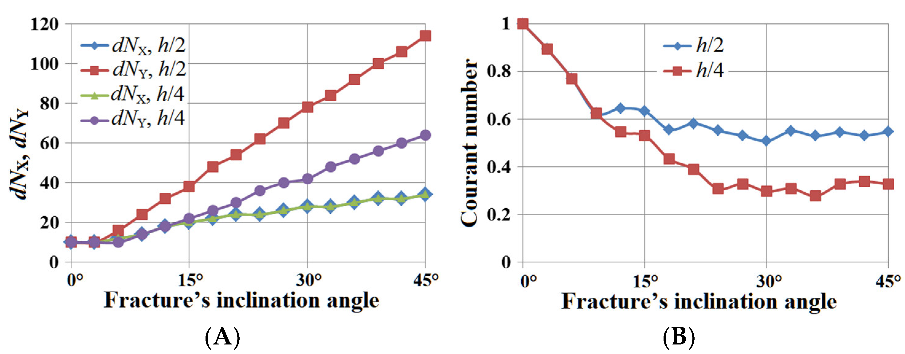
Figure 3.
(A) Graphs of on the fracture’s inclination angle , , , , , ; (B) graphs of on the fracture’s inclination angle for , , , , , .
Figure 3.
(A) Graphs of on the fracture’s inclination angle , , , , , ; (B) graphs of on the fracture’s inclination angle for , , , , , .
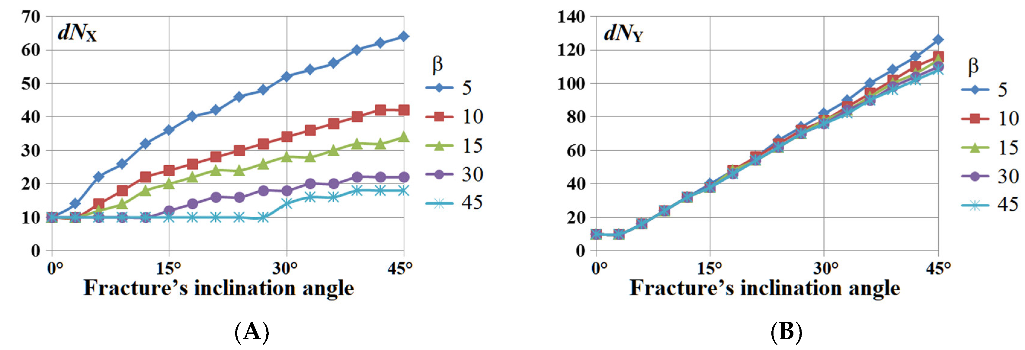
Figure 4.
Examples of structured curvilinear meshes around fractures for different fracture inclination angles: (A) 30°; (B) 45°; (C) 75°.
Figure 4.
Examples of structured curvilinear meshes around fractures for different fracture inclination angles: (A) 30°; (B) 45°; (C) 75°.

Figure 5.
Two interconvertible problem statements, the receivers’ positions are marked with the diamonds, and the source position is marked with the asterisk: (A) with an overlapping curvilinear mesh, original coordinate system; (B) without an overlapping curvilinear mesh.
Figure 5.
Two interconvertible problem statements, the receivers’ positions are marked with the diamonds, and the source position is marked with the asterisk: (A) with an overlapping curvilinear mesh, original coordinate system; (B) without an overlapping curvilinear mesh.
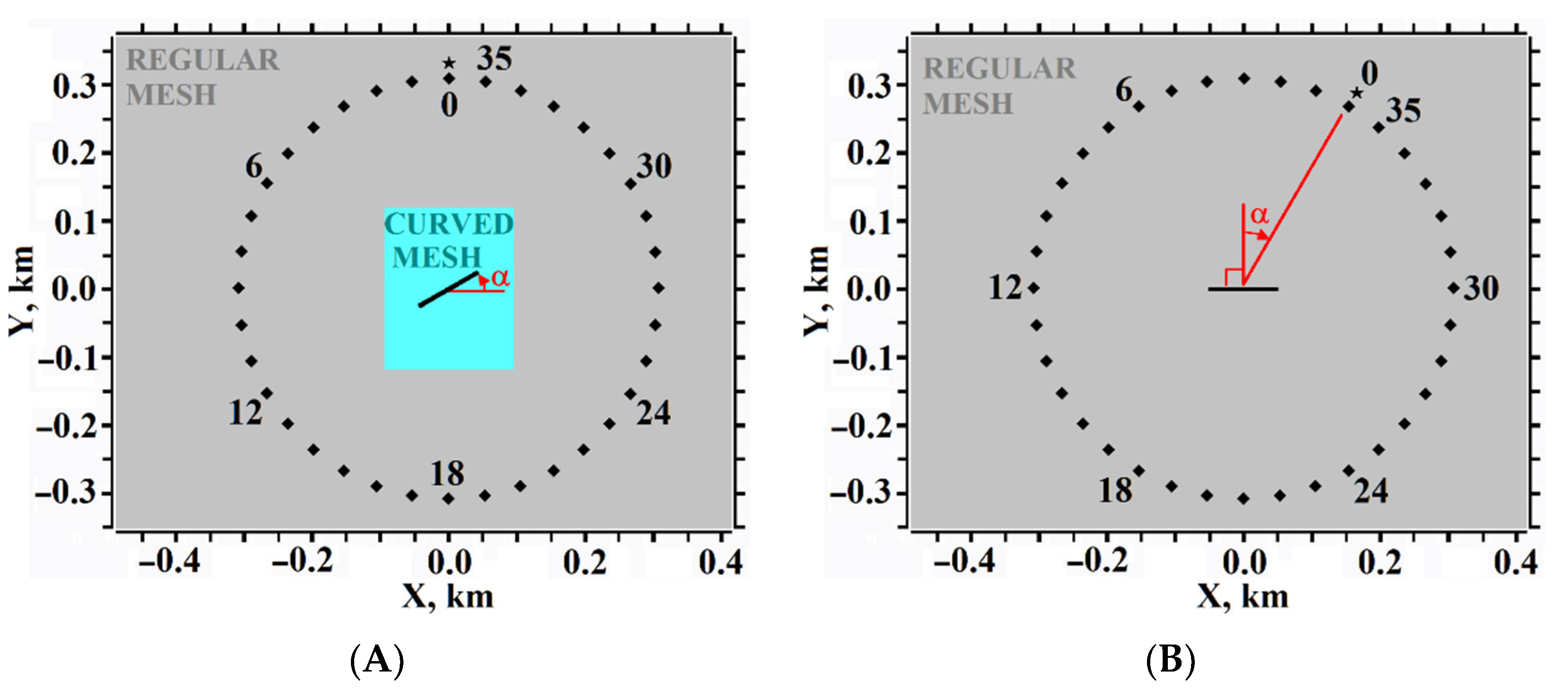
Figure 6.
Dependence of the relative errors on the angle α.
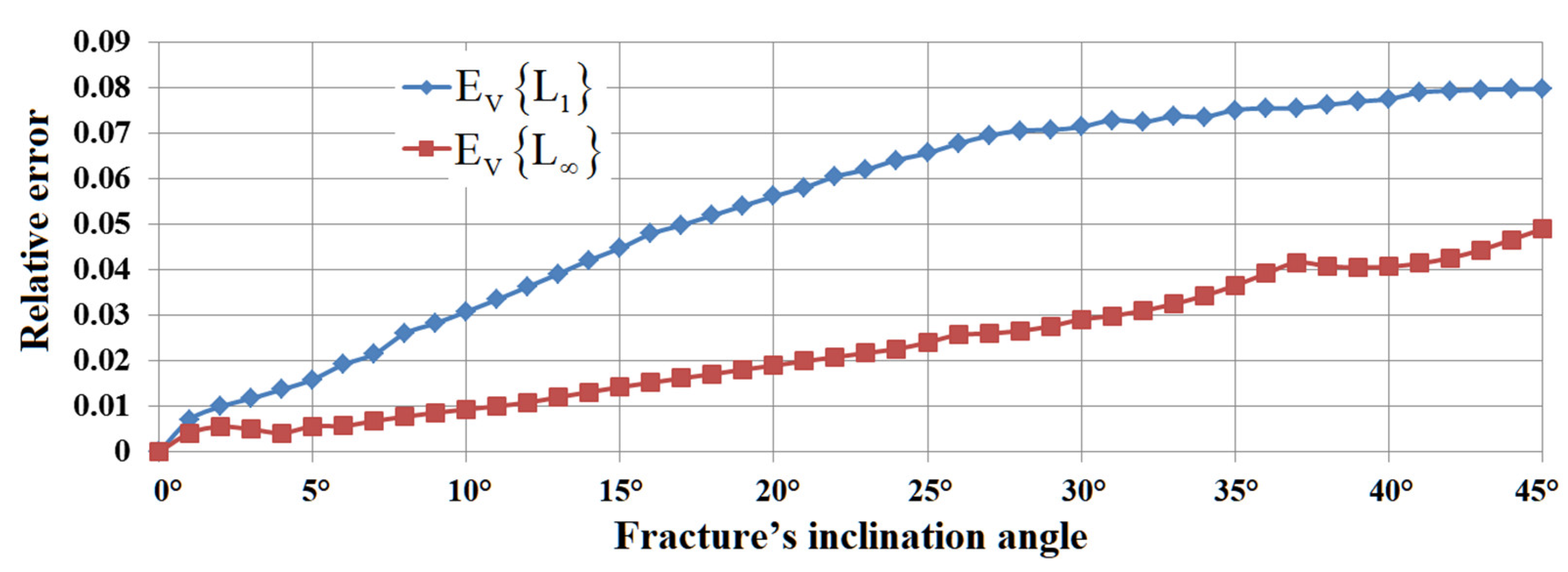
Figure 7.
Dependence of the relative errors of the anomalous velocity on the angle α.
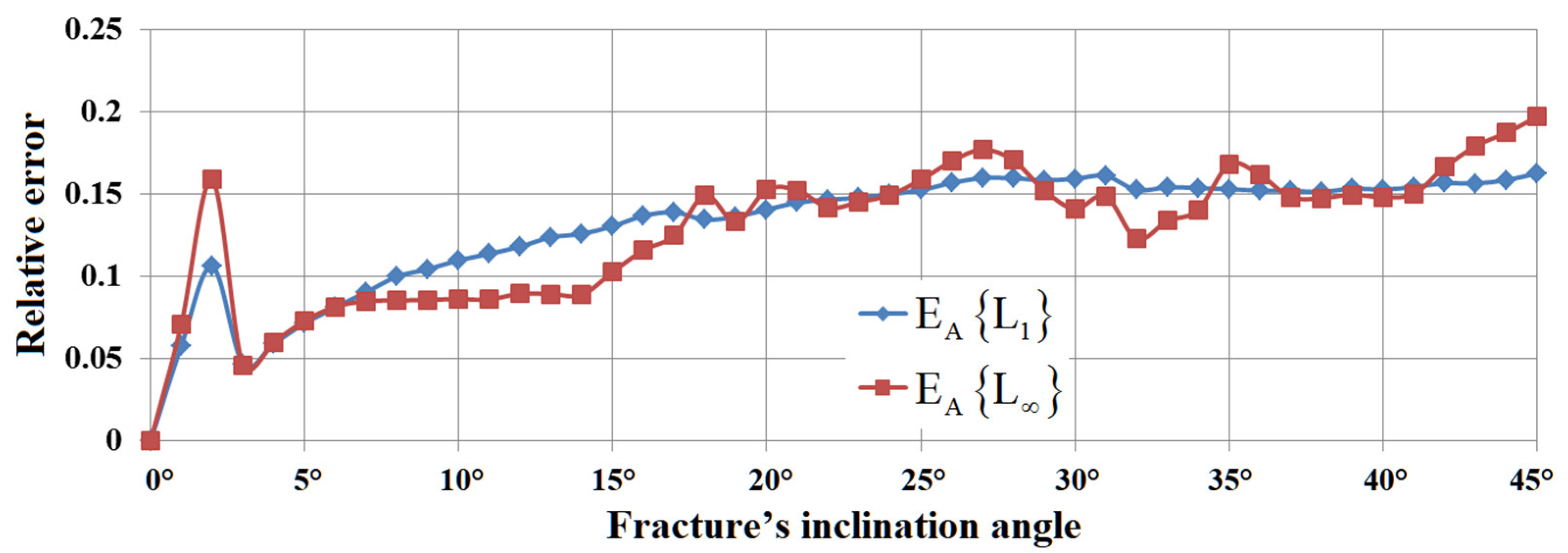
Figure 8.
Velocity modulus snapshots, time moment of 0.8 s, distance in km, diamonds mark the receivers’ positions, the asterisk denotes the source position: (A) with an overlapping curvilinear mesh;(B) without an overlapping curvilinear mesh.
Figure 8.
Velocity modulus snapshots, time moment of 0.8 s, distance in km, diamonds mark the receivers’ positions, the asterisk denotes the source position: (A) with an overlapping curvilinear mesh;(B) without an overlapping curvilinear mesh.
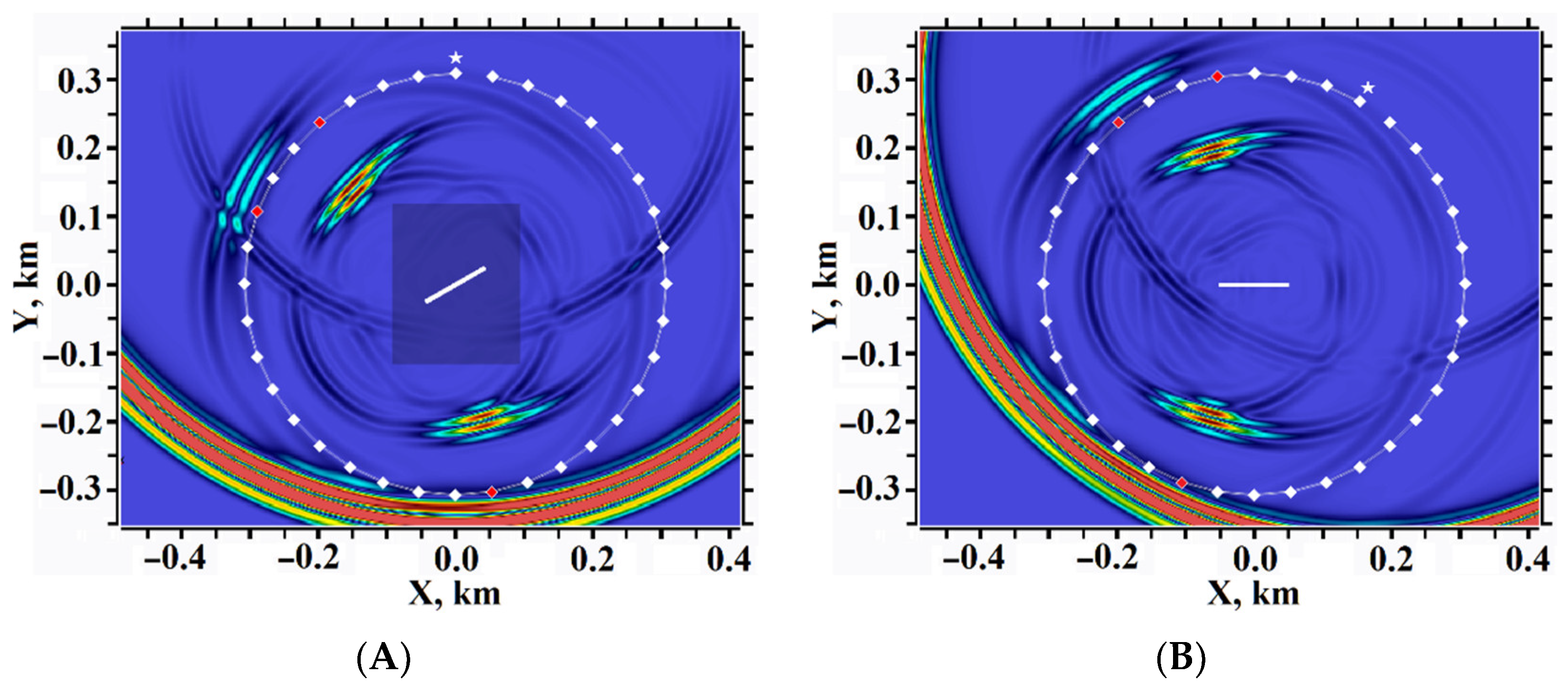
Figure 9.
Seismograms, anomalous velocity modulus: (A) with an overlapping curvilinear mesh; (B) without an overlapping curvilinear mesh; (C) difference.
Figure 9.
Seismograms, anomalous velocity modulus: (A) with an overlapping curvilinear mesh; (B) without an overlapping curvilinear mesh; (C) difference.
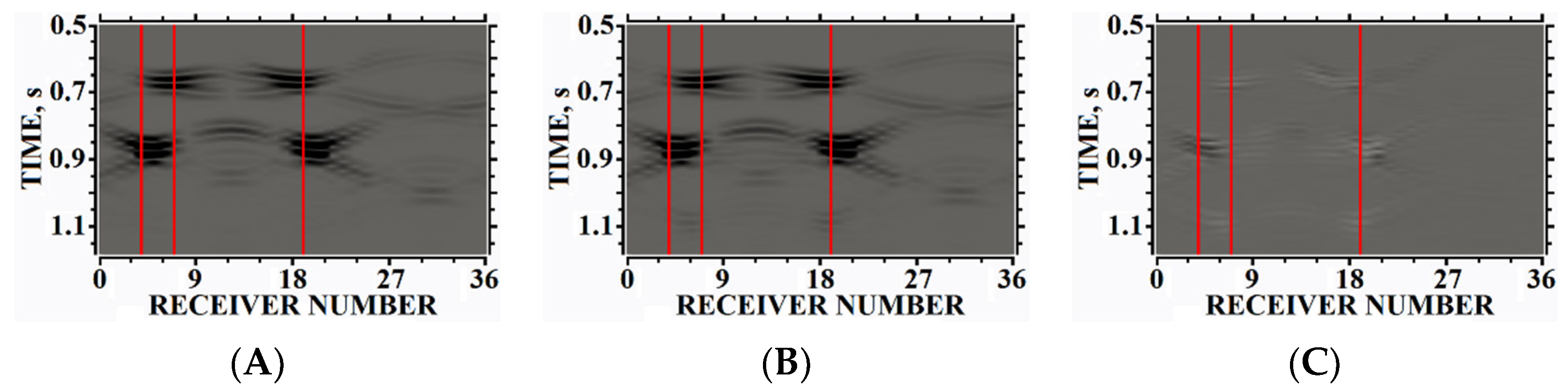
Figure 10.
Seismograms, X-component of the anomalous velocity: (A) with an overlapping curvilinear mesh; (B) without an overlapping curvilinear mesh; (C) difference.
Figure 10.
Seismograms, X-component of the anomalous velocity: (A) with an overlapping curvilinear mesh; (B) without an overlapping curvilinear mesh; (C) difference.
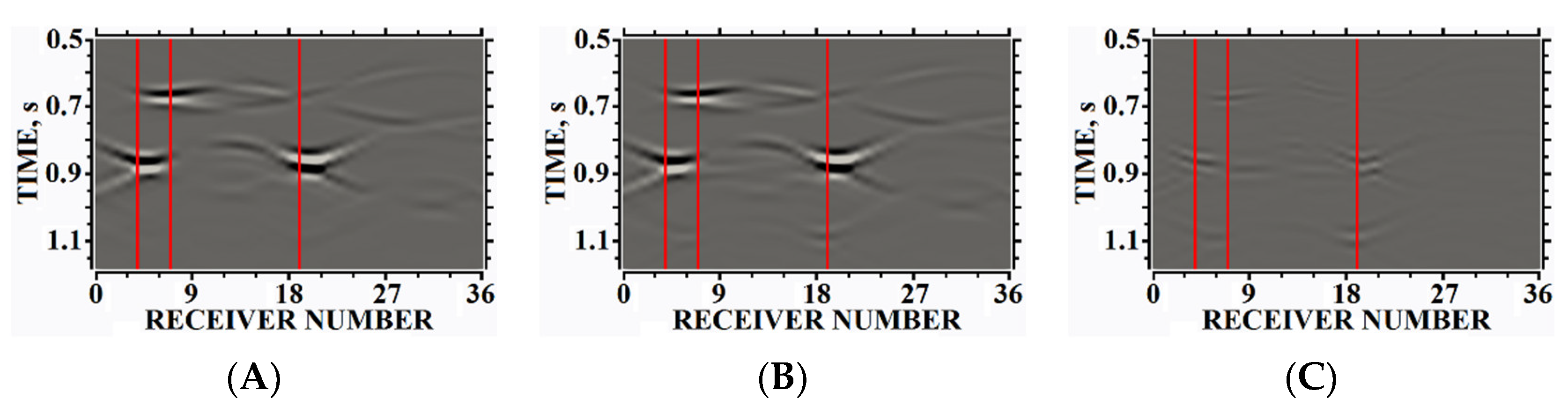
Figure 11.
Seismograms, Y-component of the anomalous velocity: (A) with overlapping curvilinear mesh; (B) without overlapping curvilinear mesh; (C) difference.
Figure 11.
Seismograms, Y-component of the anomalous velocity: (A) with overlapping curvilinear mesh; (B) without overlapping curvilinear mesh; (C) difference.
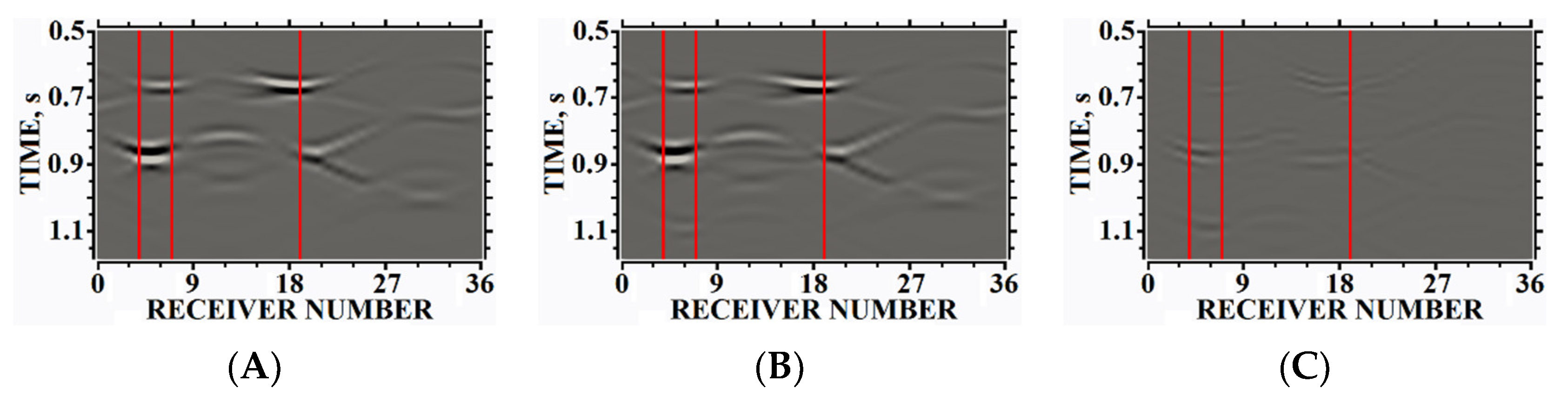
Figure 12.
Receiver #4, dependencies of velocity modulus on time.

Figure 13.
Receiver #4, dependencies of X-component of velocity on time.
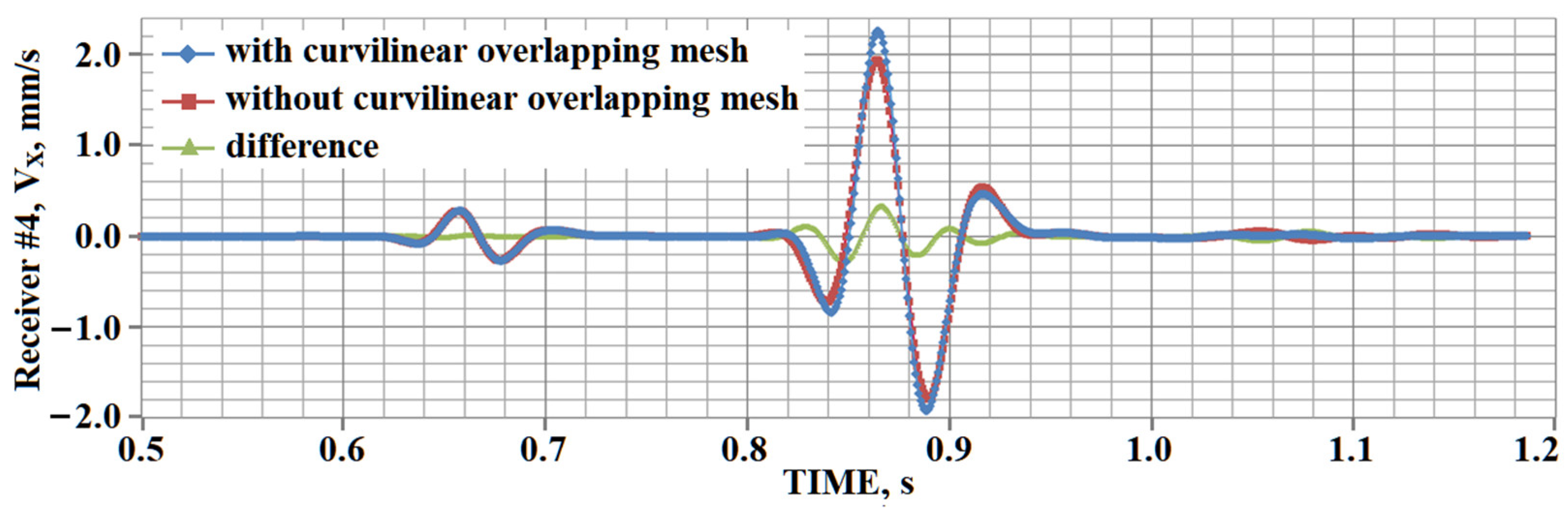
Figure 14.
Receiver #4, dependencies of Y-component of velocity on time.
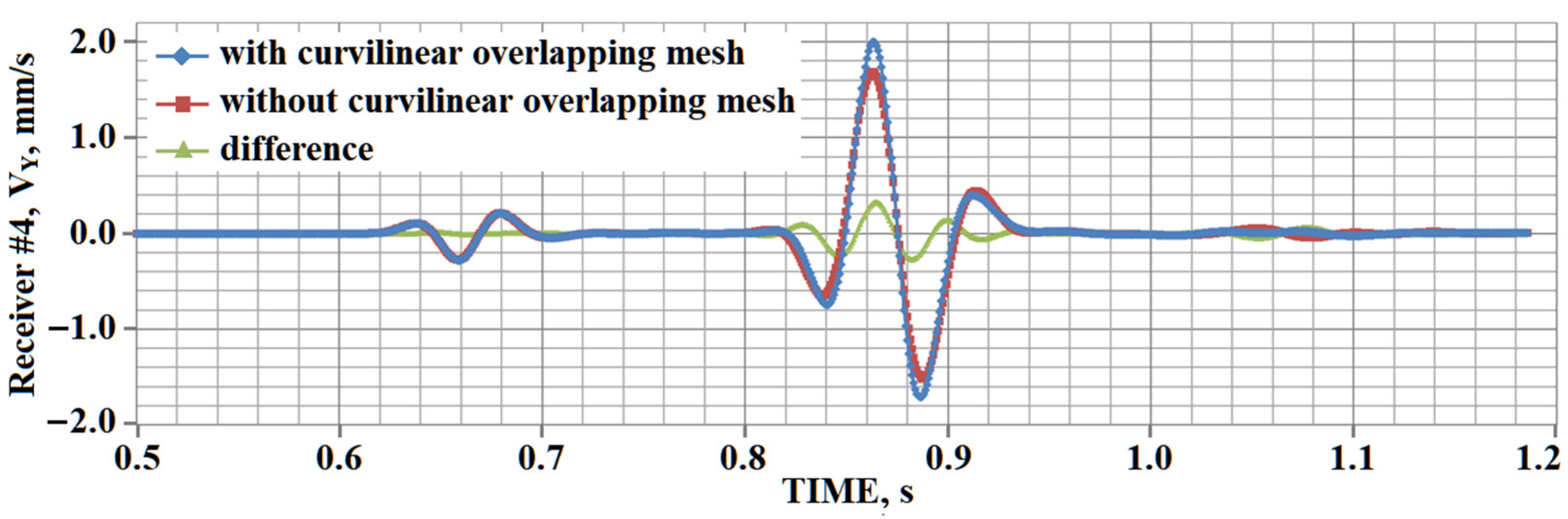
Figure 15.
Receiver #7, dependencies of velocity modulus on time.
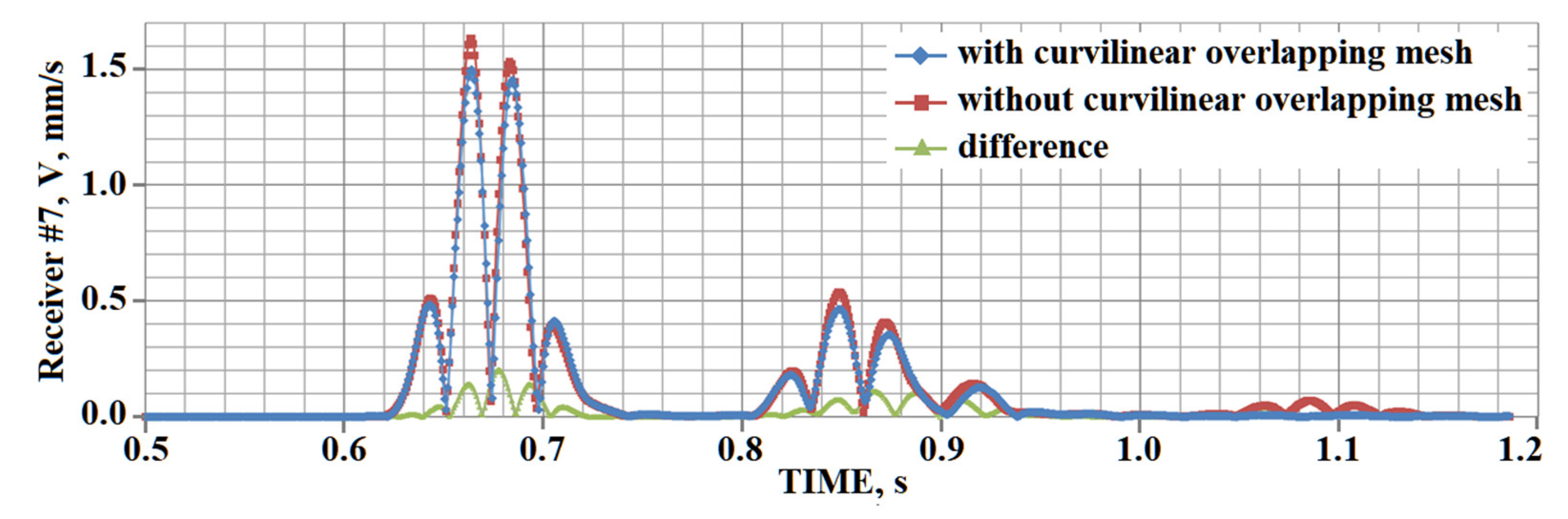
Figure 16.
Receiver #7, dependencies of X-component of velocity on time.

Figure 17.
Receiver #7, dependencies of Y-component of velocity on time.
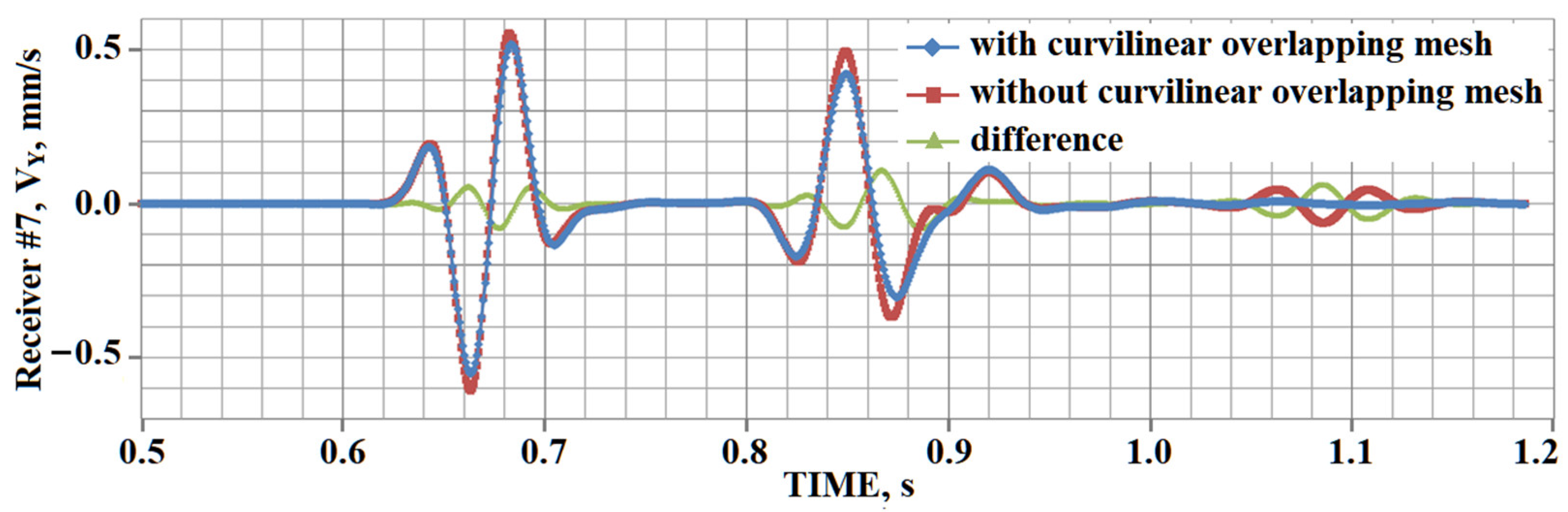
Figure 18.
Receiver #19, dependencies of velocity modulus on time.
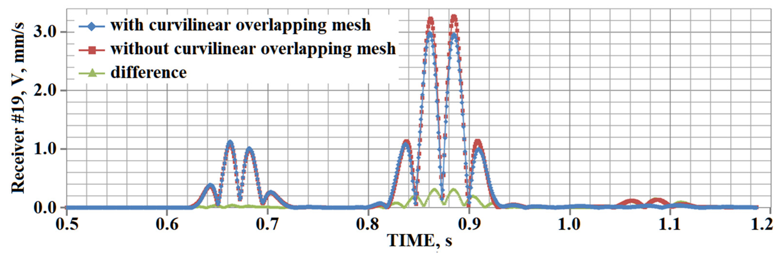
Figure 19.
Receiver #19, dependencies of X-component of velocity on time.
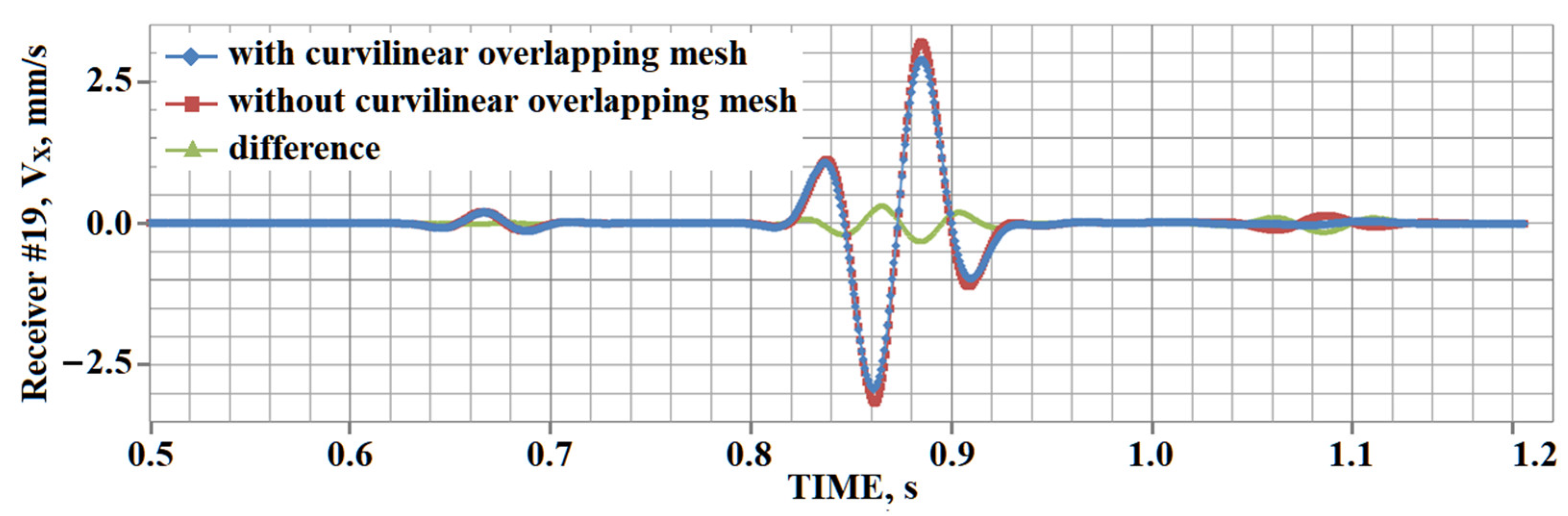
Figure 20.
Receiver #19, dependencies of Y-component of velocity on time.
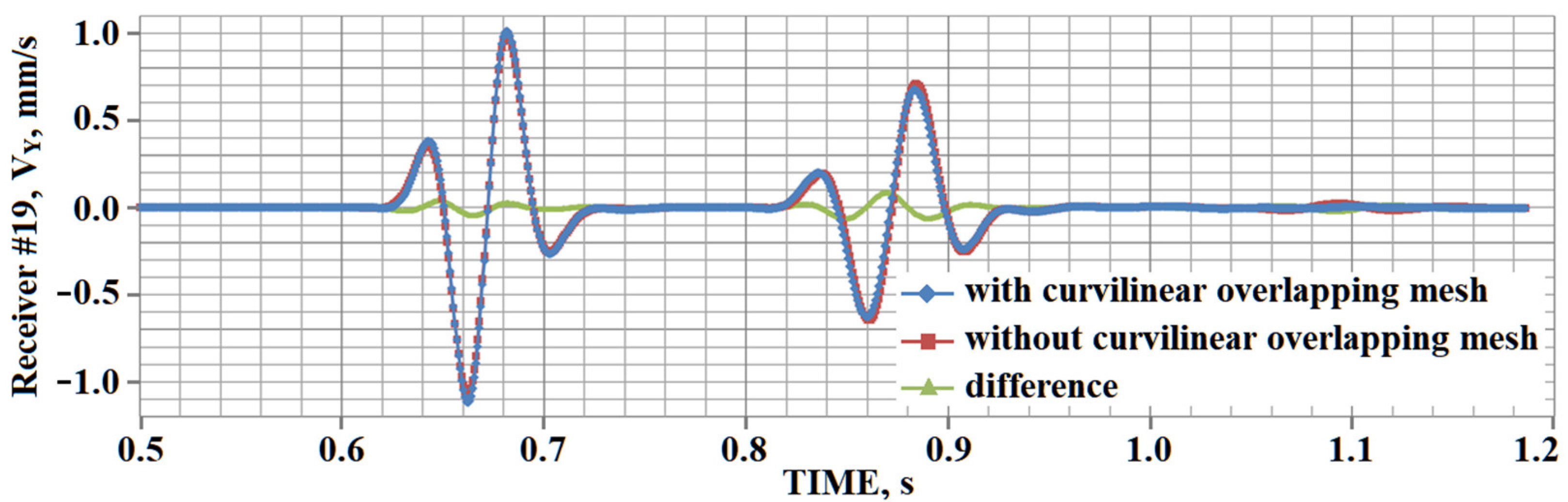
Figure 21.
Example #1, incident P-wave: (A) geophysical model, overlapping curvilinear meshes, the incident P-wave is marked with the red line; (B) velocity modulus snapshot at the time moment 0.26 s; (C) scale of the velocity modulus used in the paper.
Figure 21.
Example #1, incident P-wave: (A) geophysical model, overlapping curvilinear meshes, the incident P-wave is marked with the red line; (B) velocity modulus snapshot at the time moment 0.26 s; (C) scale of the velocity modulus used in the paper.
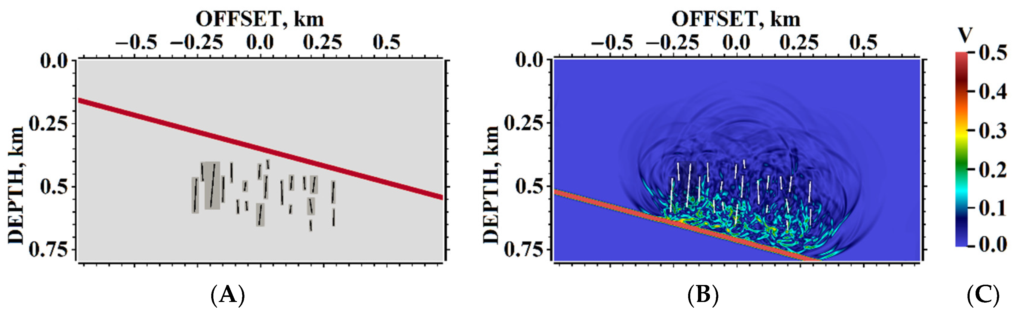
Figure 22.
Example #1, incident P-wave, snapshots at the time moment 0.26 s: (A) horizontal component of velocity; (B) vertical component of velocity; (C) scale of the velocity components used in the paper.
Figure 22.
Example #1, incident P-wave, snapshots at the time moment 0.26 s: (A) horizontal component of velocity; (B) vertical component of velocity; (C) scale of the velocity components used in the paper.
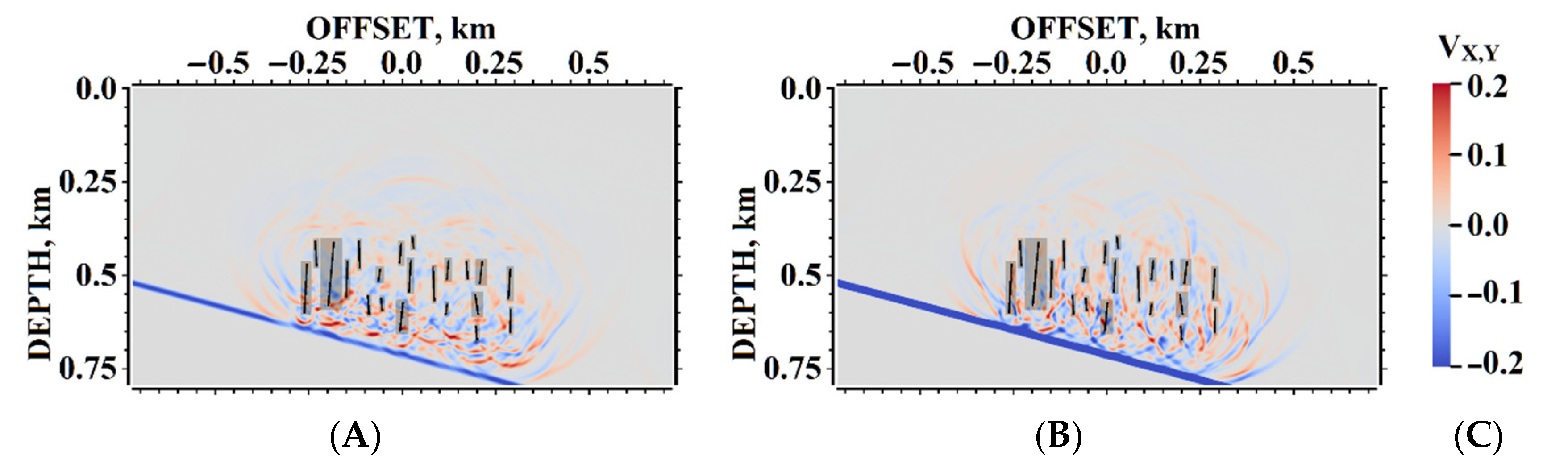
Figure 23.
Example #1, incident S-wave: (A) geophysical model, overlapping curvilinear meshes, the incident S-wave is marked with the red line; (B) velocity modulus snapshot at the time moment 0.38 s.
Figure 23.
Example #1, incident S-wave: (A) geophysical model, overlapping curvilinear meshes, the incident S-wave is marked with the red line; (B) velocity modulus snapshot at the time moment 0.38 s.
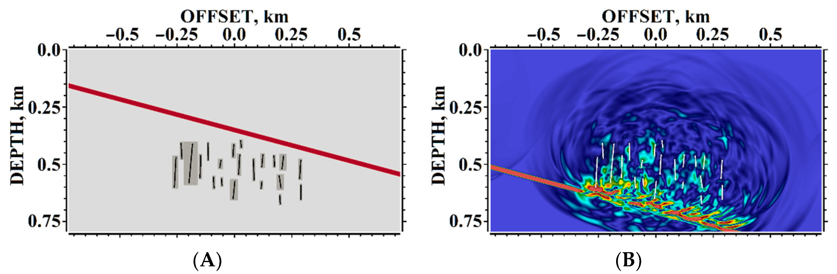
Figure 24.
Example #1, incident S-wave, snapshots at the time moment 0.38 s: (A) horizontal component of velocity; (B) vertical component of velocity.
Figure 24.
Example #1, incident S-wave, snapshots at the time moment 0.38 s: (A) horizontal component of velocity; (B) vertical component of velocity.

Figure 25.
Example #2: (A) geophysical model, overlapping curvilinear mesh, the point source is marked by the red dot; (B) velocity modulus snapshot.
Figure 25.
Example #2: (A) geophysical model, overlapping curvilinear mesh, the point source is marked by the red dot; (B) velocity modulus snapshot.

Figure 26.
Example #2, snapshots at the time moment of 0.555 s: (A) horizontal component of velocity; (B) vertical component of velocity.
Figure 26.
Example #2, snapshots at the time moment of 0.555 s: (A) horizontal component of velocity; (B) vertical component of velocity.

Figure 27.
Example #3: (A) geophysical model, overlapping curvilinear mesh, a point source is marked by the red dot; (B) velocity modulus snapshot.
Figure 27.
Example #3: (A) geophysical model, overlapping curvilinear mesh, a point source is marked by the red dot; (B) velocity modulus snapshot.

Figure 28.
Example #3, snapshots at the time moment of 0.86 s: (A) horizontal component of velocity; (B) vertical component of velocity.
Figure 28.
Example #3, snapshots at the time moment of 0.86 s: (A) horizontal component of velocity; (B) vertical component of velocity.
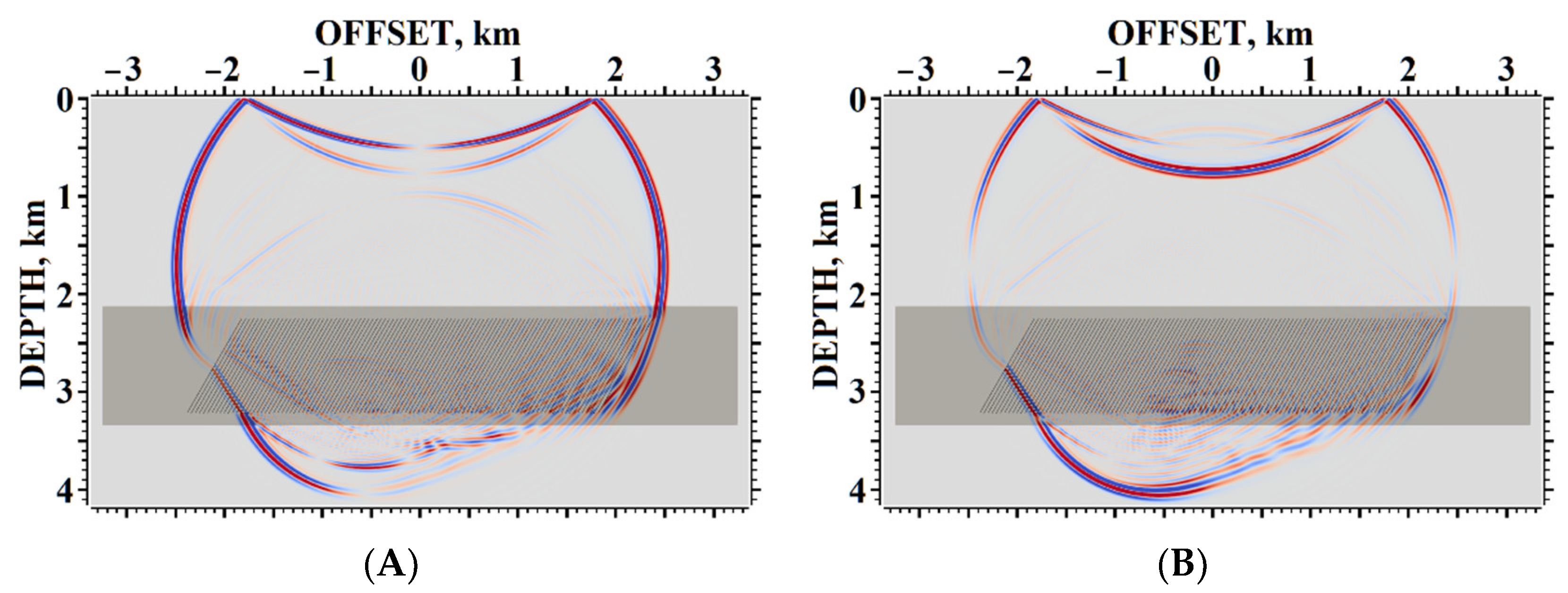
Figure 29.
Example #4: (A) scales of elastic parameters; (B) geophysical model, overlapping curvilinear meshes, the point source is marked by the red dot; (C) velocity modulus snapshot.
Figure 29.
Example #4: (A) scales of elastic parameters; (B) geophysical model, overlapping curvilinear meshes, the point source is marked by the red dot; (C) velocity modulus snapshot.
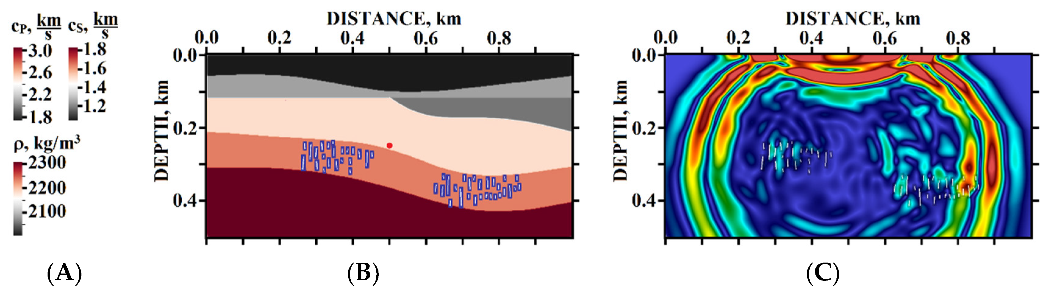
Figure 30.
Example #4, snapshots at the time of 0.25 s: (A) horizontal component of velocity; (B) vertical component of velocity.
Figure 30.
Example #4, snapshots at the time of 0.25 s: (A) horizontal component of velocity; (B) vertical component of velocity.
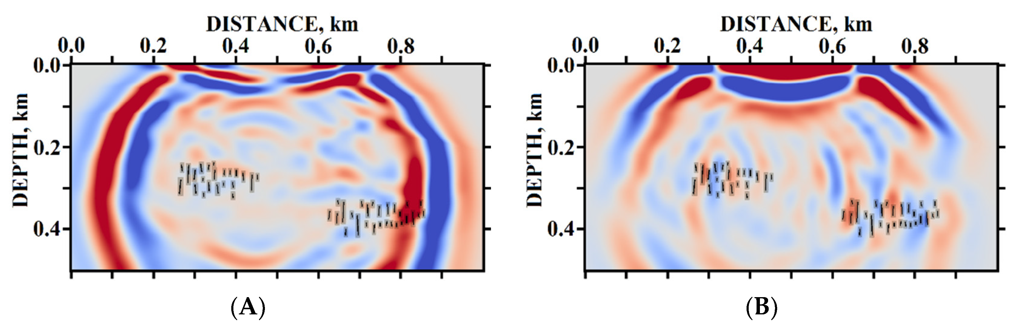
Figure 31.
Example #5: (A) geophysical model, «without fractures», the point source is marked by the red dot; (B) scales of elastic properties; (C) scales of wave field snapshots; (D) scales of seismograms.
Figure 31.
Example #5: (A) geophysical model, «without fractures», the point source is marked by the red dot; (B) scales of elastic properties; (C) scales of wave field snapshots; (D) scales of seismograms.
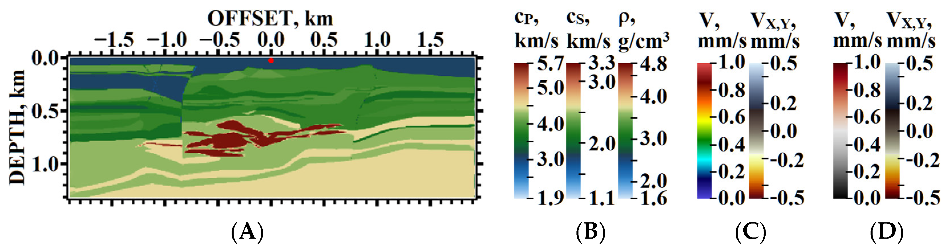
Figure 32.
Example #5, geophysical model, the point source is marked by the red dot: (A) «fractured zone #1»; (B) «fractured zone #2».
Figure 32.
Example #5, geophysical model, the point source is marked by the red dot: (A) «fractured zone #1»; (B) «fractured zone #2».
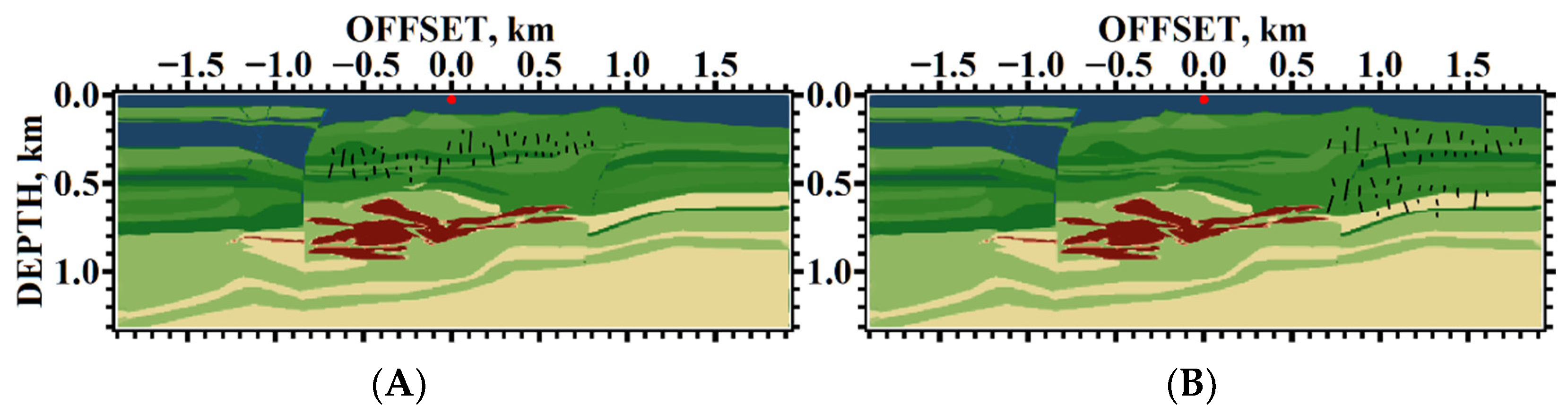
Figure 33.
Example #5, velocity modulus snapshot: (A,B) «without fractures», time of 0.275 s (A) and time of 0.51 (B); (C,D) «fractured zone #1», time of 0.2784925 s (C) and time of 0.516477 (D); (E,F) «fractured zone #2», time of 0.2695 s (E) and time of 0.4998 s (F).
Figure 33.
Example #5, velocity modulus snapshot: (A,B) «without fractures», time of 0.275 s (A) and time of 0.51 (B); (C,D) «fractured zone #1», time of 0.2784925 s (C) and time of 0.516477 (D); (E,F) «fractured zone #2», time of 0.2695 s (E) and time of 0.4998 s (F).
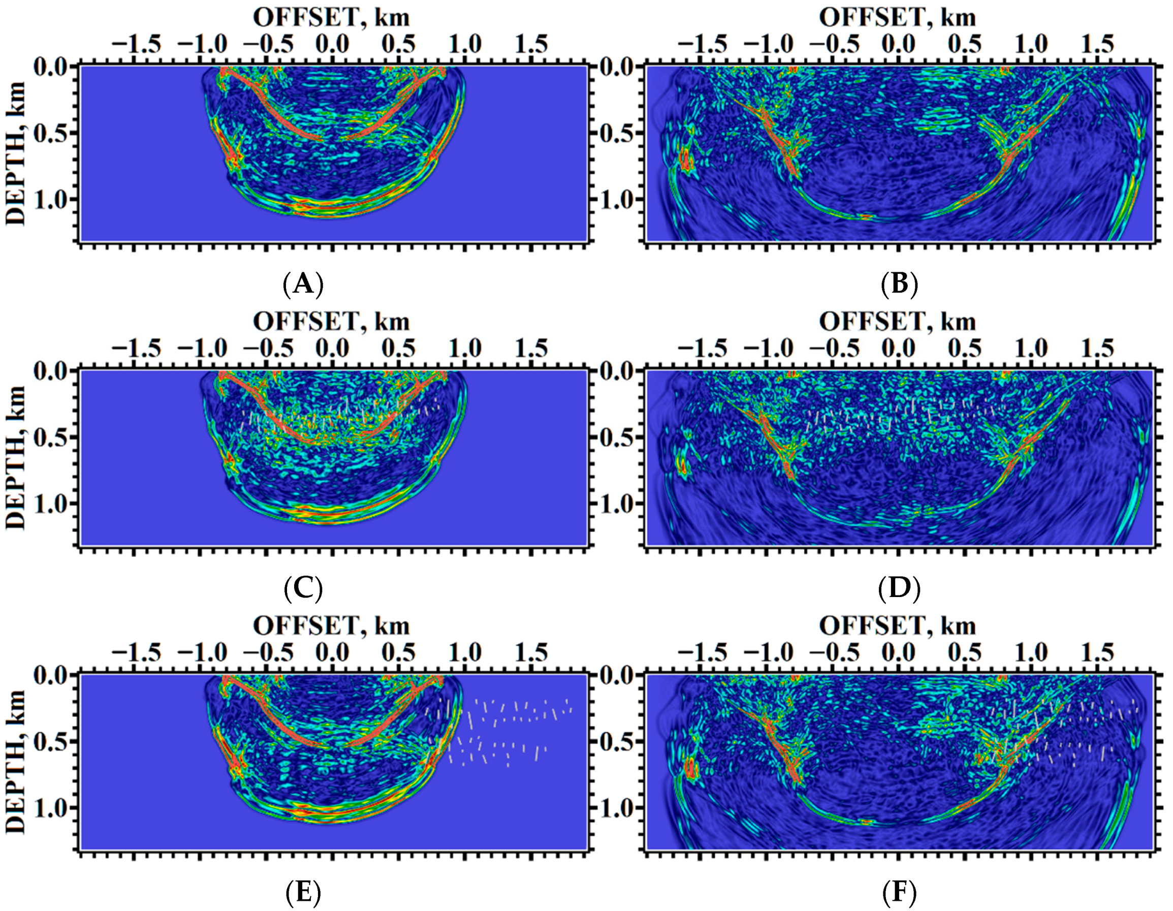
Figure 34.
Example #5, horizontal component of velocity snapshot: (A,B) «without fractures», time of 0.275 s (A) and time of 0.51 (B); (C,D) «fractured zone #1», time of 0.2784925 s (C) and time of 0.516477 (D); (E,F) «fractured zone #2», time of 0.2695 s (E) and time of 0.4998 s (F).
Figure 34.
Example #5, horizontal component of velocity snapshot: (A,B) «without fractures», time of 0.275 s (A) and time of 0.51 (B); (C,D) «fractured zone #1», time of 0.2784925 s (C) and time of 0.516477 (D); (E,F) «fractured zone #2», time of 0.2695 s (E) and time of 0.4998 s (F).
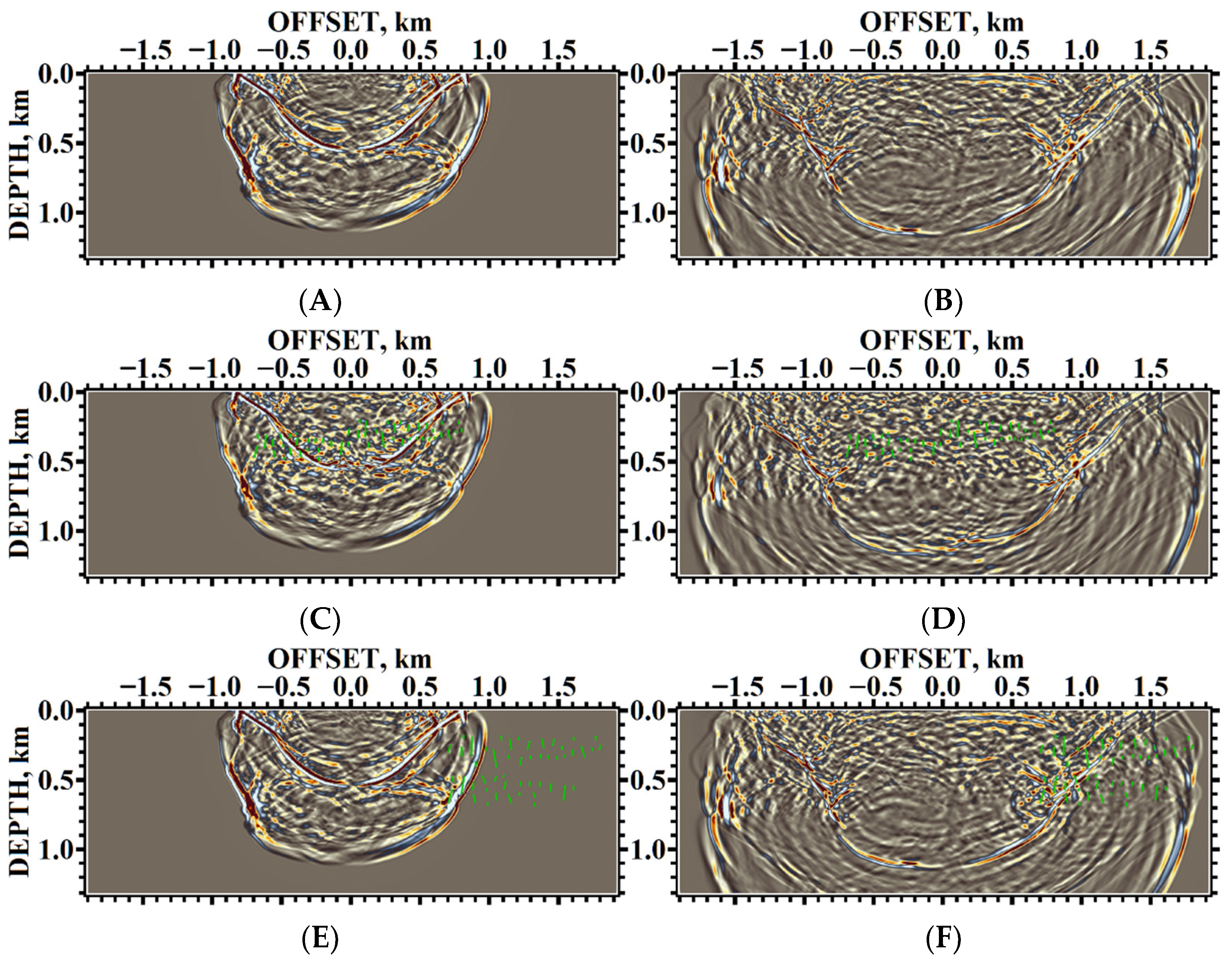
Figure 35.
Example #5, vertical component of velocity snapshot: (A,B) «without fractures», time of 0.275 s (A) and time of 0.51 (B); (C,D) «fractured zone #1», time of 0.2784925 s (C) and time of 0.516477 (D); (E,F) «fractured zone #2», time of 0.2695 s (E) and time of 0.4998 s (F).
Figure 35.
Example #5, vertical component of velocity snapshot: (A,B) «without fractures», time of 0.275 s (A) and time of 0.51 (B); (C,D) «fractured zone #1», time of 0.2784925 s (C) and time of 0.516477 (D); (E,F) «fractured zone #2», time of 0.2695 s (E) and time of 0.4998 s (F).

Figure 36.
Example #5, seismograms, velocity modulus: (A) «without fractures»; (B) «fractured zone #1»; (C) «fractured zone #2».
Figure 36.
Example #5, seismograms, velocity modulus: (A) «without fractures»; (B) «fractured zone #1»; (C) «fractured zone #2».

Figure 37.
Example #5, seismograms, vertical component of velocity: (A) «without fractures»; (B) «fractured zone #1»; (C) «fractured zone #2».
Figure 37.
Example #5, seismograms, vertical component of velocity: (A) «without fractures»; (B) «fractured zone #1»; (C) «fractured zone #2».
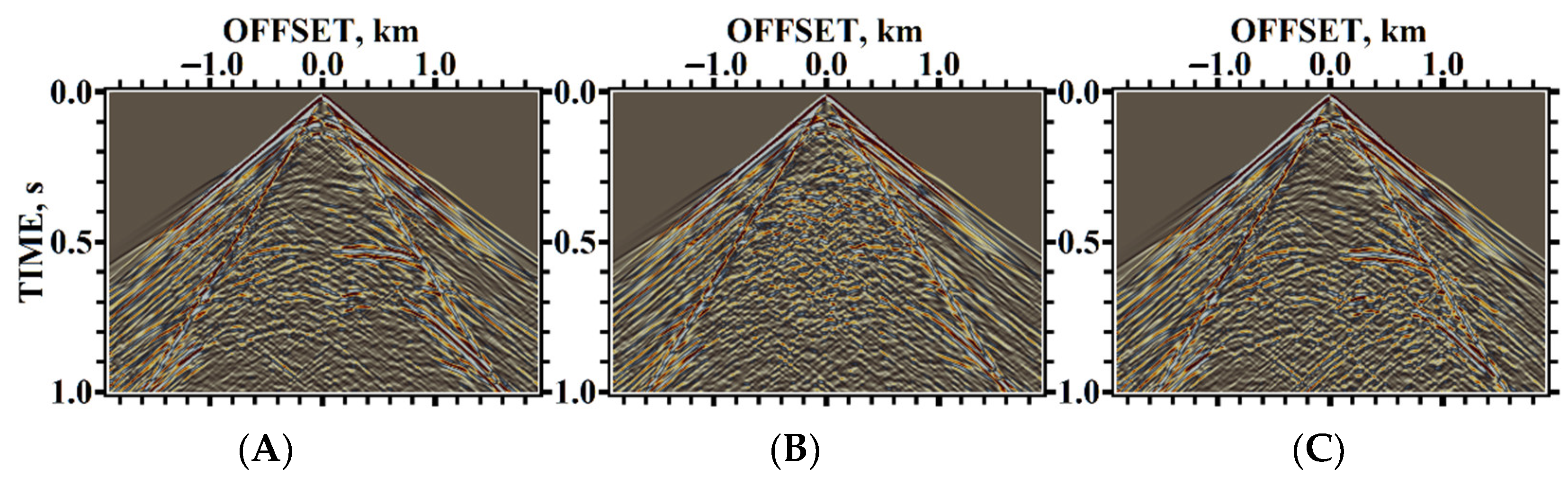
Figure 38.
Example #5, seismograms, vertical component of velocity: (A) «without fractures»; (B) «fractured zone #1»; (C) «fractured zone #2».
Figure 38.
Example #5, seismograms, vertical component of velocity: (A) «without fractures»; (B) «fractured zone #1»; (C) «fractured zone #2».
Publisher’s Note: MDPI stays neutral with regard to jurisdictional claims in published maps and institutional affiliations. |
© 2022 by the authors. Licensee MDPI, Basel, Switzerland. This article is an open access article distributed under the terms and conditions of the Creative Commons Attribution (CC BY) license (https://creativecommons.org/licenses/by/4.0/).
Share and Cite
MDPI and ACS Style
Khokhlov, N.I.; Favorskaya, A.; Furgailo, V. Grid-Characteristic Method on Overlapping Curvilinear Meshes for Modeling Elastic Waves Scattering on Geological Fractures. Minerals 2022, 12, 1597. https://doi.org/10.3390/min12121597
AMA Style
Khokhlov NI, Favorskaya A, Furgailo V. Grid-Characteristic Method on Overlapping Curvilinear Meshes for Modeling Elastic Waves Scattering on Geological Fractures. Minerals. 2022; 12(12):1597. https://doi.org/10.3390/min12121597
Chicago/Turabian StyleKhokhlov, Nikolay I., Alena Favorskaya, and Vladislav Furgailo. 2022. "Grid-Characteristic Method on Overlapping Curvilinear Meshes for Modeling Elastic Waves Scattering on Geological Fractures" Minerals 12, no. 12: 1597. https://doi.org/10.3390/min12121597
Note that from the first issue of 2016, this journal uses article numbers instead of page numbers. See further details here.