

Gravity Data Enhancement Using the Exponential Transform of the Tilt Angle of the Horizontal Gradient
by
 , ,
, ,
Luan Thanh Pham
1,
Saulo Pomponet Oliveira
2,
Cuong Van Anh Le
3,
Nhung Thi Bui
4,
An Hoa Vu
4 and
Duong Anh Nguyen
4,* 1
Department of Geophysics, Faculty of Physics, University of Science, Vietnam National University, Hanoi 100000, Vietnam
2
Graduate Program in Geology, Department of Mathematics, Federal University of Paraná, Curitiba 81531-980, PR, Brazil
3
Department of Geophysics, Faculty of Physics and Engineering Physics, University of Science, Vietnam National University, Ho Chi Minh City 700000, Vietnam
4
Institute of Geophysics, Vietnam Academy of Science and Technology, Hanoi 100000, Vietnam
*
Author to whom correspondence should be addressed.
Minerals 2023, 13(12), 1539; https://doi.org/10.3390/min13121539
Submission received: 31 October 2023
/
Revised: 1 December 2023
/
Accepted: 6 December 2023
/
Published: 11 December 2023
(This article belongs to the Special Issue Application of Geophysical Data Interpretation in Geological and Mineral Potential Mapping)
Abstract
:Detecting the boundaries of geologic structures is one of the main tasks in interpreting gravity anomalies. Many methods based on the derivatives of gravity anomalies have been introduced to map the source boundaries. The drawbacks of traditional methods are that the estimated boundaries are divergent or false boundaries appear in the output map. Here, we use the exponential transform of the tilt angle of the horizontal gradient to improve the edge detection results. The robustness of the presented method is illustrated using synthetic data and real examples from the Voisey’s Bay Ni-Cu-Co deposit (Canada) and the Tuan Giao (Vietnam). The findings show that the presented technique can produce more precise and clear boundaries.
1. Introduction
Geophysical methods are known as a powerful tool in mapping geological structures and minerals [1,2,3,4,5,6]. The gravity method is characterized by low cost and broad coverage compared to other geophysical surveys [7,8]. Interpreting gravity data provides important information about subsurface geological features [9,10,11]. The enhancement techniques of gravity anomalies can quickly determine the boundaries of the structures, and bring more abundant information for interpreting geologic formations [12,13,14,15].
Many techniques have been developed for enhancing gravity data [16,17,18,19,20,21,22]. These techniques are based on gradients of the anomalous field [23,24,25,26]. Unbalanced and balanced edge detection techniques are the two primary types of edge enhancement techniques [27]. The horizontal gradient [28], analytic signal [29], enhanced horizontal derivative [30], and analytic signals of gravity gradient tensor [31] are the unbalanced filters that are most often used for enhancing gravity data. The unbalanced methods can delineate the boundaries of shallow sources with high amplitudes, but they have limited detection effects on the boundaries of low amplitude anomalies [12,32].
To outline the boundaries of sources located at different depths, some balanced techniques have been developed. Most of these methods have been based on trigonometric functions, such as the tilt angle [33], theta map [34], exponential transform of the theta map [35], and normalized horizontal gradient [36]. A second generation of these methods involved high-order derivatives, for example, the tilt angle of the horizontal gradient [37], horizontal directional theta map [38], the horizontal gradient of the Ntilt [39], directional theta [40], logistic functions [41,42], enhanced horizontal gradient [43], and horizontal gradient of the improved normalized horizontal gradient [44]. The effectiveness of the edge detection techniques in terms of their precision in the determination of edges has been estimated in some recent studies [45,46,47,48]. Most of these studies showed that the tilt angle of the horizontal gradient is a powerful tool in mapping geological structures, but its edge map has a low resolution [46,47,48].
In this paper, we present a method to improve the edge detection results. Our method uses the exponential transform of the tilt angle of the horizontal gradient to bring the edge detection results with a high resolution and avoid producing additional edges in the output map. The application of the presented method is shown on real examples from the Voisey’s Bay Ni-Cu-Co deposit (Canada) and the Tuan Giao (Vietnam).
2. Method
The theta map is a popular method in edge detection of potential field data, which normalizes the horizontal gradient by the analytic signal [34]. This method is defined as:
where F is the gravity field.
To delineate the source boundaries more clearly, in 2013, Li suggested using the exponential transform of the theta map that is given by [35]:
where p is a constant decided by the interpreter. The use of p = 4 or 8 can make the edges more clearly [35]. The maxima of the ETM correspond to the source edges. Although the ETM can improve the resolution of the TM, it does not remove false edges in the edge map of the TM.
Another popular method is the tilt angle of the horizontal gradient that is given by [37]:
where the horizontal gradient (HG) is given by:
Although the use of the TAHG can avoid bringing false information, its estimated boundaries are divergent. Here, we follow Li [35] to improve the resolution of the tilt angle of the horizontal gradient. The method is defined as:
The maxima of the ETAHG correspond to the source edges. Similar to the TAHG, it does not produce false information in the edge map. However, it can yield the edges with a higher resolution compared to the TAHG.
3. Methods Used for Comparison
To estimate the robustness of the presented method, we compared it to popular methods such as the horizontal gradient (HG), analytic signal amplitude (AS), theta map (TM), and some recent methods such as the exponential transform of the TM (ETM), tilt angle of the horizontal gradient (TAHG), horizontal gradient of NTilt (HGNTilt) and horizontal gradient of impTDX (HGimpTDX). The HG, TM, ETM and TAHG formulas are given in Section 2, while the AS, HGNTilt and HGimpTDX are shortly summarized below.
The AS is one of the most commonly used filters, which uses the peaks to extract the edges, and is defined as [29]:
The HGNTilt uses the horizontal gradient of the NTilt to enhance the edges. The method is given by [39]:
where NTilt is defined as:
with and k given by:
and M is the regional gravity value.
4. Results and Discussion
4.1. Synthetic Examples
In this section, we estimate the effectiveness of the ETAHG through synthetic gravity examples with and without noise. The synthetic model includes five prisms, as shown in Figure 1a. The parameters of the model are presented in Table 1. Using these parameters, the gravity anomaly of the model is calculated and shown in Figure 1b.
In the first example, we applied the selected methods to gravity data in Figure 1b. Figure 2a presents the result of the HG method. It can be observed that the HG cannot equalize the different anomalies. The HG can determine the edges of the sources P2 and P3, but responses from other sources are faint. Figure 2b displays the edges outlined by the AS. It is observed that the AS is less effective in mapping the edges of the thin or deep sources. The results obtained from the method are fairly faint. Figure 2c presents the edges determined by the TM method. The method can equalize anomalies with different amplitudes, but it generates some false edges around the body P4. Figure 2c displays the edges determined by the ETM with p = 1. It is obvious that the ETM result is similar to the TM but has a higher resolution. The ETM was also computed using p = 4 (Figure 2e) and 8 (Figure 2f), as recommended in [35]. Clearly, the use of the ETM with p = 8 can generate sharper signals over the edges but the edge information of the body P1 is lost. Figure 2g,f display the edges delineated by the HGNTilt and HGimpTDX methods, respectively. Both methods generate the edges with a very high resolution, but some additional edges appear in the output maps of these methods. Figure 2i presents the edges determined by the TAHG method. Although the method can detect all the edges, the edges obtained from this method are divergent. Figure 2j–o display the edges delineated by the ETAHG with p = 1, 2, 3, 4, 6 and 8, respectively. As can be observed from these figures, the ETAHG maps have a higher resolution compared to the TAHG. Although the resolution of the ETAHG map increases when using larger values of p, the edges of the body P1 are lost or faint.
The results of the TAHG and ETAHG from Figure 2 were also compared in a horizontal profile (Figure 1b). Figure 3a shows the gravity anomaly along this profile. Figure 3b–h display the edges determined by the TAHG and ETAHG with p = 1, 2, 3, 4, 6 and 8, respectively. One can note from these figures that the signals over the edges along the ETAHG profiles are sharper than those of the TAHG. However, the amplitude of the transformed signal over the source P1 decreases as the p value increases. The ETAHG produces weak amplitude responses when the p value is greater than or equal to 2. For this reason, we used p = 1 in the subsequent ETAHG calculations.
To estimate the sensitivity of the ETAHG to random noise, we consider the second example where gravity data in Figure 2b was corrupted with 3% Gaussian noise (Figure 4a). Figure 5a–h display the edges delineated by applying the HG, AS, TM, ETM, HGNTilt, HGimpTDX, TAHG and ETAHG to gravity data in Figure 4a, respectively. As can be observed from these figures, the HG and AS are less sensitive to noise than others. However, these methods are dominated by the bodies P2 and P3. The TM, ETM, HGNTilt, HGimpTDX, TAHG and ETAHG are less sensitive to the depth of the bodies. As the HGNTilt and HGimpTDX are based on the third derivatives and/or fourth derivatives, they are more sensitive to noise than the TM, ETM, TAHG and ETAHG. In this case, the ETAHG still shows the edges more clearly than other methods.
Since the enhancement techniques of gravity data are based on derivatives of the field, they amplify the noise. To attenuate the noise effect, the noise-corrupted data were subjected to an upward continuation filter of 1 km before using the techniques (Figure 4b). Figure 6a–h present the edges delineated by applying the HG, AS, TM, ETM, HGNTilt, HGimpTDX, TAHG and ETAHG to gravity data in Figure 4b, respectively. It is obvious that the HG can clearly outline the edges of the bodies P2 and P3, but the responses over the other sources are faint (Figure 6a). The AS cannot outline the edges of the dike P1 and deep sources P4 and P5 (Figure 6b). The ETM shows sharper edges than the TM, but both methods still generate false boundaries around the body P4 (Figure 6c,d). Although the HGNTilt and HGimpTDX can determine most of the edges with a very high resolution, some additional edges still appear along the north-south edges of the body G1, and around the body P4 output maps of these methods (Figure 6e,f). The TAHG and ETAHG can highlight all the source boundaries without any false information. However, the ETAHG generates higher resolution boundaries of the sources.
4.2. Real Examples
4.2.1. Voisey’s Bay Ni-Cu-Co Deposit
One of the most important mineral discoveries in Canada over the last few decades is the Voisey’s Bay Ni–Cu–Co deposit, which is situated on the northeast coast of Labrador (Figure 7) [49]. The primary ore body is the ovoid that is being mined at the moment (Figure 7). With horizontal dimensions of 650 by 350 m and a maximum depth extension of 120 m, it is a massive sulphide lens with an elliptical shape. It is estimated that there are 30 million tons of proven and probable reserves, grading 2.9% nickel, 1.7% copper, and 0.14% cobalt [49]. The deposit is linked to the Voisey’s Bay intrusion, which crosses the 1.85 Ga east-dipping collisional boundary between the Archean Nain Province to the east and the Proterozoic Churchill Province to the west (Figure 7) [50,51].
The Bouguer gravity map of the Voisey’s Bay is shown in Figure 8a [52]. The Bouguer gravity map of the Voisey’s Bay comprises the primary ore body. Figure 8b–i present the edges delineated by applying the HG, AS, TM, ETM, HGNTilt, HGimpTDX, TAHG and ETAHG to gravity data in Figure 8a, respectively. It can be observed that the peaks of the HG, HGNTilt, HGimpTDX, TAHG and ETAHG demonstrated the presence of a primary ore body with an approximate ellipsoidal form, as reported by some other studies (Figure 8b,f–i) [49,53]. However, the HG and TAHG results are divergent. The HGNTilt and HGimpTDX are very effective in providing high resolution boundaries, but they bring some additional boundaries at the edges of the study area. In this case, the AS does not provide a clear image of the main ore body (Figure 8c), while the TM and ETM bring false maxima in the northeastern region. Comparing the results, one can observe that the ETAHG does not yield additional edges, and it can provide the edges more clearly compared to others.
4.2.2. Tuan Giao Area
The Tuan Giao area is located between the South China block and the Sundaland block. It is considered as a part of the transition boundary zone between these two blocks [54]. Two main factors, the (i) collision of the Indo-Australian and Eurasian plates and (ii) subduction of the Pacific plate under Eurasian plate, explain that the Tuan Giao area has high dynamic activities. The Tuan Giao is a mountainous area with a complicated geological structure (Figure 9), dominated by many active faults, such as the Dien Bien Phu fault, Son La fault, Song Da fault and Song Ma fault [55,56,57]. From the works of many researchers, young materials (i.e., magmatic rocks) intruded into old sedimentary rocks environment through the faults (Figure 9) [55,56]. For this area, Permian–Triassic sediment rocks dominate the most area while the rest as thin stripes disseminate along faults. In this area, there were at least seven earthquakes, with a magnitude of above five occurring from 1914 to 1983. These earthquakes are shown in Figure 5. The two biggest earthquakes occurred at Dien Bien in 1935 (M 6.8) and Tuan Giao in 1983 (M 6.7) (Figure 9). Both earthquakes severely damaged homes and infrastructure and killed or injured dozens of people in landslides [54]. Since then, no earthquakes with a magnitude of 5 have occurred in the study area; thus, this is a high-risk area for earthquakes. Therefore, accurately determining the location of faults in high-risk earthquake areas is necessary to have accurate earthquake hazard assessments and earthquake forecasts in the area.
Figure 10a displays the Bouguer gravity map of the Tuan Giao [58]. Figure 10b–i display the boundaries delineated by applying the HG, AS, TM, ETM, HGNTilt, HGimpTDX, TAHG and ETAHG to Bouguer gravity data in Figure 10a, respectively. One can observe that the HG and AS are dominated by anomalies at the northern part of the area, and these methods do not yield images of the structural boundaries. The obtained image maps from the application of the TM, ETM, HGNTilt, HGimpTDX and TAHG allow us to extract the structural boundaries, and show the boundaries of the large and small signals clearly (Figure 10d–h). While the edges in the TM, ETM and TAHG are divergent, the HGNTilt and HGimpTDX produce very sharp edges. However, the use of the HGNTilt and HGimpTDX may bring some additional edges, as shown in the synthetic examples. In this case, the edges determined by the ETAHG are more precise and clearer (Figure 10i). It can be observed from Figure 10i that the ETAHG map shows a dominant NW-SE structural trend of density bodies that correspond favorably to the geological formations of the Tuan Giao. In addition, the maximum locations in the ETAHG map exhibit a strong correlation with a large number of NW-NW-SE trending faults in the region.
5. Conclusions
In this paper, we have presented an improved method to extract the edges of gravity data. The method uses the exponential transform of the tilt angle of the horizontal gradient to enhance the edges. The theoretical tests show that the presented method can extract the edges of shallow and deep bodies simultaneously. In addition, this method produces results with more precise and clear boundaries compared to other methods. The application of the presented method is illustrated in mapping structures of the Tuan Giao (Vietnam) and boundaries of the Voisey’s Bay Ni-Cu-Co deposit (Canada). The findings from the real examples are in agreement with the known structures of the study areas. Assuming that the magnetization direction is known, we can compute RTP magnetic data. Then, the presented method can be used for interpreting magnetic data.
Author Contributions
Conceptualization, L.T.P.; methodology, L.T.P. and S.P.O.; software, L.T.P. and S.P.O.; validation, N.T.B., A.H.V. and D.A.N.; investigation, L.T.P., S.P.O., C.V.A.L., N.T.B., A.H.V. and D.A.N.; data curation, N.T.B., A.H.V. and D.A.N.; writing—original draft preparation, L.T.P., S.P.O., C.V.A.L. and D.A.N.; writing—review and editing, L.T.P., S.P.O., C.V.A.L., N.T.B., A.H.V. and D.A.N.; supervision, C.V.A.L., S.P.O. and D.A.N. All authors have read and agreed to the published version of the manuscript.
Funding
This research was funded by PAS-VAST, QTPL01.01/22-23; and CNPq, 316376/2021-3.
Data Availability Statement
The data presented in this study are available on reasonable request from the corresponding author.
Acknowledgments
Authors thank for the result discussion of Phan Trong Trinh and the support of the senior researcher, NVCC 11.01/22-23. The authors thank two anonymous reviewers for their constructive comments.
Conflicts of Interest
The authors declare no conflict of interest.
References
- Ai, H.; Ekinci, Y.L.; Balkaya, Ç.; Essa, K.S. Inversion of geomagnetic anomalies caused by ore masses using Hunger Games Search algorithm. Earth Space Sci. 2023, 10, e2023EA003002. [Google Scholar] [CrossRef]
- Sampietro, D.; Capponi, M.; Maurizio, G. 3D Bayesian inversion of potential fields: The Quebec Oka carbonatite complex case study. Geosciences 2022, 12, 382. [Google Scholar] [CrossRef]
- Boszczuk, P.; Cheng, L.Z.; Hammouche, H.; Roy, P.; Lacroix, S.; Cheilletz, A. A 3D gravity data interpretation of the Matagami mining camp, Abitibi Subprovince, Superior Province, Québec, Canada: Application to VMS deposit exploration. J. Appl. Geophys. 2011, 75, 77–86. [Google Scholar] [CrossRef]
- Wijanarko, E.; Arisbaya, I.; Sumintadireja, P.; Grandis, H. Magnetotellurics study of Atambua area, West Timor, Indonesia. Vietnam J. Earth Sci. 2022, 45, 67–81. [Google Scholar] [CrossRef] [PubMed]
- Xayavong, V.; Duc, M.V.; Singsoupho, S.; Anh, D.N.; Prasad, K.N.D.; Minh, T.V.; Do Anh, C. Combination of 2D-Electrical Resistivity Imaging and Seismic Refraction Tomography methods for groundwater potential assessments: A case study of Khammouane province, Laos. Vietnam J. Earth Sci. 2023, 45, 238–250. [Google Scholar] [CrossRef] [PubMed]
- Marques, F.; Matos, J.X.; Sousa, P.; Represas, P.; Araujo, A.; Carvalho, J.; Morais, I.; Pacheco, N.; Albardeiro, L.; Goncalves, P. The role of land gravity data in the Neves-Corvo mine discovery and its use in present-day exploration and new target generation. First Break 2019, 37, 97–102. [Google Scholar] [CrossRef]
- Nabighian, M.N.; Ander, M.E.; Grauch, V.J.S.; Hansen, R.O.; LaFehr, T.R.; Li, Y.; Pearson, W.C.; Peirce, J.W.; Phillips, J.D.; Ruder, M.E. Historical development of the gravity method in exploration. Geophysics 2005, 70, 63–89. [Google Scholar] [CrossRef]
- Hinze, W.; Frese, R.; Saad, A. Gravity and Magnetic Exploration: Principles, Practices, and Applications; Cambridge University Press: Cambridge, UK, 2013. [Google Scholar]
- Narayan, S.; Kumar, U.; Pal, S.K.; Sahoo, S.D. New insights into the structural and tectonic settings of the Bay of Bengal using high-resolution earth gravity model data. Acta Geophys. 2021, 69, 2011–2033. [Google Scholar] [CrossRef]
- Narayan, S.; Sahoo, S.D.; Pal, S.K.; Kumar, U. Comparative evaluation of five global gravity models over a part of the Bay of Bengal. Adv. Space Res. 2022, 71, 2416–2436. [Google Scholar] [CrossRef]
- Oksum, E. Grav3CH_inv: A GUI-based MATLAB code for estimating the 3-D basement depth structure of sedimentary basins with vertical and horizontal density variation. Comput. Geosci. 2021, 155, 104856. [Google Scholar] [CrossRef]
- Kamto, P.G.; Oksum, E.; Pham, L.T.; Kamguia, J. Contribution of advanced edge detection filters for the structural mapping of the Douala Sedimentary Basin along the Gulf of Guinea. Vietnam J. Earth Sci. 2023, 45, 287–302. [Google Scholar]
- Narayan, S.; Sahoo, S.D.; Pal, S.K.; Kumar, U.; Pathak, V.K.; Majumdar, T.J.; Chouhan, A. Delineation of structural features over a part of the Bay of Bengal using total and balanced horizontal derivative techniques. Geocarto Int. 2016, 32, 351–366. [Google Scholar] [CrossRef]
- Ekinci, Y.L.; Yigitbas, E. Interpretation of gravity anomalies to delineate some structural features of Biga and Gelibolu peninsulas, and their surroundings (north-west Turkey). Geodin. Acta 2015, 27, 300–319. [Google Scholar] [CrossRef]
- Eldosouky, A.M.; El-Qassas, R.A.Y.; Pham, L.T.; Abdelrahman, K.; Alhumimidi, M.S.; El Bahrawy, A.; Mickus, K.; Sehsah, H. Mapping Main Structures and Related Mineralization of the Arabian Shield (Saudi Arabia) Using Sharp Edge Detector of Transformed Gravity Data. Minerals 2022, 12, 71. [Google Scholar] [CrossRef]
- Melouah, O.; Ebong, E.D.; Abdelrahman, K.; Eldosouky, A.M. Lithospheric structural dynamics and geothermal modeling of the Western Arabian Shield. Sci. Rep. 2023, 13, 11764. [Google Scholar] [CrossRef] [PubMed]
- Kumar, U.; Pal, S.K.; Sahoo, S.D.; Narayan, S.; Saurabh, M.S.; Ganguli, S.S. Lineament mapping over Sir Creek offshore and its surroundings using high resolution EGM2008 gravity data: An integrated derivative approach. J. Geol. Soc. India 2018, 91, 671–678. [Google Scholar] [CrossRef]
- Melouah, O.; Eldosouky, A.M.; Ebong, W.D. Crustal architecture, heat transfer modes and geothermal energy potentials of the Algerian Triassic provinces. Geothermics 2021, 96, 102211. [Google Scholar] [CrossRef]
- Prasad, K.N.D.; Pham, L.T.; Singh, A.P. A novel filter “ImpTAHG” for edge detection and a case study from Cambay Rift Basin, India. Pure Appl. Geophys. 2022, 179, 2351–2364. [Google Scholar] [CrossRef]
- Cooper, G.R.J. Novel Second-Order Derivative-Based Filters for Edge and Ridge/Valley Detection in Geophysical Data. Minerals 2023, 13, 1229. [Google Scholar] [CrossRef]
- Cooper, G.R.J. Amplitude-Balanced Edge Detection Filters for Potential Field Data. Explor. Geophys. 2023, 54, 544–552. [Google Scholar] [CrossRef]
- Kafadar, Ö. Applications of the Kuwahara and Gaussian filters on potential field data. J. Appl. Geophys. 2022, 198, 104583. [Google Scholar] [CrossRef]
- Ekinci, Y.L.; Yiğitbaş, E. A geophysical approach to the igneous rocks in the Biga Peninsula (NW Turkey) based on airborne magnetic anomalies: Geological implications. Geodin. Acta 2012, 25, 267–285. [Google Scholar] [CrossRef]
- Sahoo, S.D.; Narayan, S.; Pal, S.K. Fractal analysis of lineaments using CryoSat-2 and Jason-1 satellite-derived gravity data: Evidence of a uniform tectonic activity over the middle part of the Central Indian Ridge. Phys. Chem. Earth 2022, 128, 103237. [Google Scholar] [CrossRef]
- Yuan, Y.; Yu, Q. Edge detection in potential-field gradient tensor data by use of improved horizontal analytic signal methods. Pure Appl. Geophys. 2015, 172, 461–472. [Google Scholar] [CrossRef]
- Eldosouky, A.M.; Mohamed, H. Edge detection of aeromagnetic data as effective tools for structural imaging at Shilman area, South Eastern Desert, Egypt. Arab. J. Geosci. 2021, 14, 1–10. [Google Scholar] [CrossRef]
- Eldosouky, A.M.; Pham, L.T.; Duong, V.H.; Ghomsi, F.E.K.; Henaish, A. Structural interpretation of potential field data using the enhancement techniques: A case study. Geocarto Int. 2022, 37, 16900–16925. [Google Scholar] [CrossRef]
- Cordell, L. Gravimetric expression of graben faulting in Santa Fe Country and the Espanola Basin. In 30th Field Conference, Socorro, NM, USA, 4–6 October 1979: New Mexico Geological Society Guidebook; New Mexico Geological Society: Socorro, NM, USA, 1979; pp. 59–64. [Google Scholar]
- Roest, W.R.; Verhoef, J.; Pilkington, M. Magnetic interpretation using the 3-D analytic signal. Geophysics 1992, 57, 116–125. [Google Scholar] [CrossRef]
- Fedi, M.; Florio, G. Detection of potential fields source boundaries by enhanced horizontal derivative method. Geophys. Prospect. 2001, 49, 40–58. [Google Scholar] [CrossRef]
- Beiki, M. Analytic signals of gravity gradient tensor and their application to estimate source location. Geophysics 2010, 75, 159–174. [Google Scholar] [CrossRef]
- Alvandi, A.; Ardestani, V.E. Edge detection of potential field anomalies using the Gompertz function as a high-resolution edge enhancement filter. Bull. Geophys. Oceanogr. 2023, 64, 279–300. [Google Scholar]
- Miller, H.G.; Singh, V. Potential field tilt a new concept for location of potential field sources. J. Appl. Geophys. 1994, 32, 213–217. [Google Scholar] [CrossRef]
- Wijns, C.; Perez, C.; Kowalczyk, P. Theta map: Edge detection in magnetic data. Geophysics 2005, 70, 39–43. [Google Scholar] [CrossRef]
- Li, L. Improved edge detection tools in the interpretation of potential field data. Explor. Geophys. 2013, 44, 128–132. [Google Scholar] [CrossRef]
- Cooper, G.; Cowan, D. Enhancing potential field data using filters based on the local phase. Comput. Geosci. 2006, 32, 1585–1591. [Google Scholar] [CrossRef]
- Ferreira, F.J.F.; de Souza, J.; Bongiolo, A.B.S.; de Castro, L.G. Enhancement of the total horizontal gradient of magnetic anomalies using the tilt angle. Geophysics 2013, 78, 33–41. [Google Scholar] [CrossRef]
- Yuan, Y.; Gao, J.Y.; Chen, L.N. Advantages of horizontal directional Theta method to detect the edges of full tensor gravity gradient data. J. Appl. Geophys. 2016, 130, 53–61. [Google Scholar] [CrossRef]
- Nasuti, Y.; Nasuti, A.N. Tilt as an improved enhanced tilt derivative filter for edge detection of potential field anomalies. Geophys. J. Int. 2018, 214, 36–45. [Google Scholar] [CrossRef]
- Zareie, V.; Moghadam, R.H. The application of theta method to potential field gradient tensor data for edge detection of complex geological structures. Pure Appl. Geophys. 2019, 176, 4983–5001. [Google Scholar] [CrossRef]
- Pham, L.T.; Oksum, E.; Do, T.D. Edge enhancement of potential field data using the logistic function and the total horizontal gradient. Acta Geod. Geophys. 2019, 54, 143–155. [Google Scholar] [CrossRef]
- Pham, L.T.; Vu, T.V.; Le, T.S.; Trinh, P.T. Enhancement of potential field source boundaries using an improved logistic filter. Pure Appl. Geophys. 2020, 177, 5237–5249. [Google Scholar] [CrossRef]
- Pham, L.T.; Eldosouky, A.M.; Oksum, E.; Saada, S.A. A new high resolution filter for source edge detection of potential field data. Geocarto Int. 2022, 37, 3051–3068. [Google Scholar] [CrossRef]
- Ibraheem, I.M.; Tezkan, B.; Ghazala, H.; Othman, A.A. A New Edge Enhancement Filter for the Interpretation of Magnetic Field Data. Pure Appl. Geophys. 2023, 180, 2223–2240. [Google Scholar] [CrossRef]
- Ekinci, Y.L.; Ertekin, C.; Yigitbas, E. On the effectiveness of directional derivative based filters on gravity anomalies for source edge approximation: Synthetic simulations and a case study from the Aegean graben system (western Anatolia, Turkey). J. Geophys. Eng. 2013, 10, 035005. [Google Scholar] [CrossRef]
- Pham, L.T.; Oksum, E.; Kafadar, O.; Trinh, P.T.; Nguyen, D.V.; Vo, Q.T.; Le, S.T.; Do, T.D. Determination of subsurface lineaments in the Hoang Sa islands using enhanced methods of gravity total horizontal gradient. Vietnam J. Earth Sci. 2022, 44, 395–409. [Google Scholar]
- Nasuti, Y.; Nasuti, A.; Moghadas, D. STDR: A novel approach for enhancing and edge detection of potential field data. Pure Appl. Geophys. 2019, 176, 827–841. [Google Scholar] [CrossRef]
- Liu, J.; Li, S.; Jiang, S.; Wang, X.; Zhang, J. Tools for Edge Detection of Gravity Data: Comparison and Application to Tectonic Boundary Mapping in the Molucca Sea. Surv. Geophys. 2023, 44, 1781–1810. [Google Scholar] [CrossRef]
- Farquharson, C.G.; Ash, M.R.; Miller, H.G. Geologically constrained gravity inversion for the Voisey’s Bay ovoid deposit. Lead. Edge 2008, 27, 64–69. [Google Scholar] [CrossRef]
- Li, C.; Naldrett, A. Geology and petrology of the Voisey’s Bay intrusion: Reaction of olivine with sulfide and silicate liquids. Lithos 1999, 47, 1–31. [Google Scholar] [CrossRef]
- Ryan, B. Geological Map of the Nain Plutonic Suite and Surrounding Rocks Nain-Nutak, NTS 14SW. Geological Survey Branch, Newfoundland Department of Mines and Energy, Scale 1:500,000; Government of Newfoundland and Labrador: St. John’s, NL, Canada, 1990.
- King, A. Review of Geophysical Technology for Ni-Cu-PGE deposits. In Proceedings of the Exploration 07: Fifth Decennial International Conference on Mineral Exploration, Toronto, ON, Canada, 9–12 September 2007; Milkereit, B., Ed.; CVRD Exploration Canada Inc.: Cliff, ON, Canada, 2007; pp. 647–665. [Google Scholar]
- Lelièvre, P.; Carter-McAuslan, A.; Farquharson, C.; Hurich, C. Unified geophysical and geological 3D Earth models. Lead. Edge 2012, 31, 322–328. [Google Scholar] [CrossRef]
- Duong, N.A.; Sagiya, T.; Kimata, F.; Tran, D.T.; Vy, Q.H.; Cong, D.C.; Binh, N.X.; Xuyen, N.D. Contemporary horizontal crustal movement estimation for northwestern Vietnam inferred from repeated GPS measurements. Earth Planets Space 2013, 65, 1399–1410. [Google Scholar] [CrossRef]
- Zhou, M.F.; Chen, W.T.; Wang, C.Y.; Prevec, S.A.; Liu, P.P.; Howarth, G.H. Two stages of immiscible liquid separation in the formation of Panzhihua-type Fe–Ti–V oxide deposits, SW China. Geosci. Front. 2013, 4, 481–502. [Google Scholar] [CrossRef]
- Roger, F.; Maluski, H.; Lepvrier, C.; Van, T.V.; Paquette, J.-L. LA-ICPMS zircons U/Pb dating of Permo-Triassic and Cretaceous magmatisms in Northern Vietnam–Geodynamical implications. J. Asian Earth Sci. 2012, 48, 72–82. [Google Scholar] [CrossRef]
- Tran, T.A.; Tran-Trong, H.; Pham-Ngoc, C.; Shellnutt, J.G.; Pham, T.T.; Izokh, A.E.; Pham, P.L.T.; Duangpaseuth, S.; Soulintone, O. Petrology of the Permian-Triassic granitoids in Northwest Vietnam and their relation to the amalgamation of the Indochina and Sino-Vietnam composite terranes. Vietnam J. Earth Sci. 2022, 44, 343–368. [Google Scholar] [CrossRef] [PubMed]
- Pham, L.T. A comparative study on different methods for calculating gravity effect of an uneven layer: Application to computation of Bouguer gravity anomaly in the East Vietnam Sea and adjacent areas. VNU J. Sci. Math Phys. 2020, 36, 106–114. [Google Scholar]
Figure 1.
(a) The model. (b) Gravity anomaly of the model. The gray line denotes a profile.

Figure 2.
Results of data in Figure 1b. (a) HG. (b) AS. (c) TM. (d) ETM with p = 1. (e) ETM with p = 4. (f) ETM with p = 8. (g) HGNTilt. (h) HGimpTDX. (i) TAHG. (j) ETAHG with p = 1. (k) ETAHG with p = 2. (l) ETAHG with p = 3. (m) ETAHG with p = 4. (n) ETAHG with p = 6. (o) ETAHG with p = 8.
Figure 2.
Results of data in Figure 1b. (a) HG. (b) AS. (c) TM. (d) ETM with p = 1. (e) ETM with p = 4. (f) ETM with p = 8. (g) HGNTilt. (h) HGimpTDX. (i) TAHG. (j) ETAHG with p = 1. (k) ETAHG with p = 2. (l) ETAHG with p = 3. (m) ETAHG with p = 4. (n) ETAHG with p = 6. (o) ETAHG with p = 8.
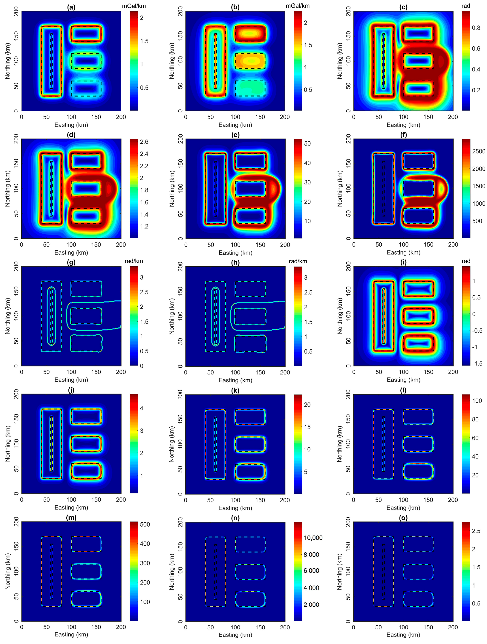
Figure 3.
(a) Gravity data along the profile in Figure 1b. (b) TAHG. (c) ETAHG with p = 1. (d) ETAHG with p = 2. (e) ETAHG with p = 3. (f) ETAHG with p = 4. (g) ETAHG with p = 6. (h) ETAHG with p = 8.
Figure 3.
(a) Gravity data along the profile in Figure 1b. (b) TAHG. (c) ETAHG with p = 1. (d) ETAHG with p = 2. (e) ETAHG with p = 3. (f) ETAHG with p = 4. (g) ETAHG with p = 6. (h) ETAHG with p = 8.

Figure 4.
(a) Gravity data corrupted with 3% Gaussian noise. (b) Upward continued gravity data.

Figure 5.
Results of data in Figure 4a. (a) HG. (b) AS. (c) TM. (d) ETM with p = 4. (e) HGNTilt. (f) HGimpTDX. (g) TAHG. (h) ETAHG with p = 1.
Figure 5.
Results of data in Figure 4a. (a) HG. (b) AS. (c) TM. (d) ETM with p = 4. (e) HGNTilt. (f) HGimpTDX. (g) TAHG. (h) ETAHG with p = 1.
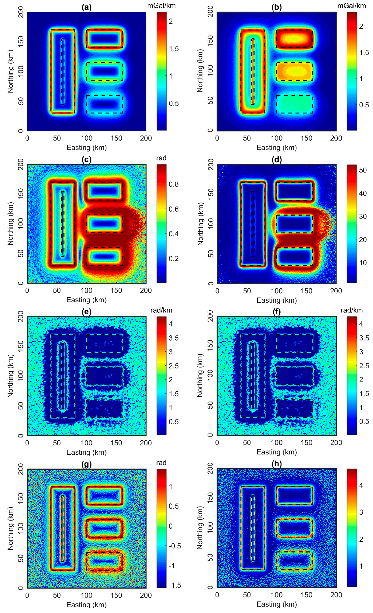
Figure 6.
Results of data in Figure 4b. (a) HG. (b) AS. (c) TM. (d) ETM with p = 4. (e) HGNTilt. (f) HGimpTDX. (g) TAHG. (h) ETAHG with p = 1.
Figure 6.
Results of data in Figure 4b. (a) HG. (b) AS. (c) TM. (d) ETM with p = 4. (e) HGNTilt. (f) HGimpTDX. (g) TAHG. (h) ETAHG with p = 1.

Figure 7.
Geology of the Voisey’s Bay area showing the location of the Voisey’s Bay Ni-Cu-Co deposit (red star) (adapted from [50,51]).
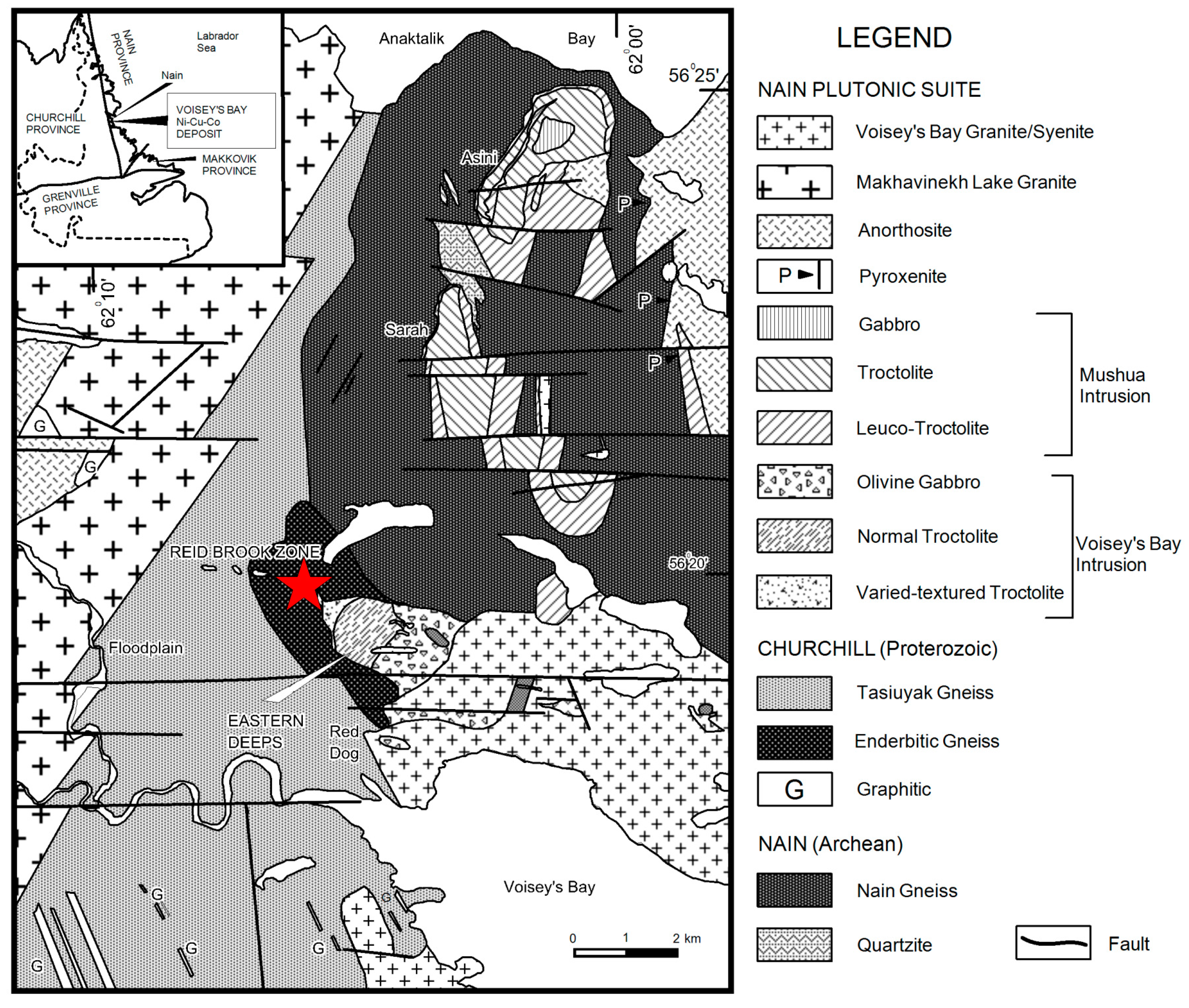
Figure 8.
(a) Bouguer data of the Voisey’s Bay Ni–Cu–Co deposit. (b) HG. (c) AS. (d) TM. (e) ETM with p = 4. (f) HGNTilt. (g) HGimpTDX. (h) TAHG. (i) ETAHG with p = 1.
Figure 8.
(a) Bouguer data of the Voisey’s Bay Ni–Cu–Co deposit. (b) HG. (c) AS. (d) TM. (e) ETM with p = 4. (f) HGNTilt. (g) HGimpTDX. (h) TAHG. (i) ETAHG with p = 1.

Figure 9.
Geology map of the Tuan Giao [55].
Figure 9.
Geology map of the Tuan Giao [55].

Figure 10.
(a) Bouguer data of the Tuan Giao. (b) HG. (c) AS. (d) TM. (e) ETM with p = 4. (f) HGNTilt. (g) HGimpTDX. (h) TAHG. (i) ETAHG with p = 1.
Figure 10.
(a) Bouguer data of the Tuan Giao. (b) HG. (c) AS. (d) TM. (e) ETM with p = 4. (f) HGNTilt. (g) HGimpTDX. (h) TAHG. (i) ETAHG with p = 1.


Table 1.
Parameters of the model.
| Parameters | P1 | P2 | P3 | P4 | P5 |
|---|---|---|---|---|---|
| Center coordinates (km; km) | 60; 100 | 60; 100 | 130; 155 | 130; 100 | 130; 45 |
| Width (km) | 4 | 40 | 30 | 30 | 30 |
| Length (km) | 110 | 140 | 60 | 60 | 60 |
| Depth of top (km) | 2 | 3 | 3 | 6 | 9 |
| Depth of bottom (km) | 3 | 5 | 7 | 10 | 13 |
| Density contrast (g/cm3) | 0.2 | 0.3 | 0.2 | −0.2 | 0.2 |
Disclaimer/Publisher’s Note: The statements, opinions and data contained in all publications are solely those of the individual author(s) and contributor(s) and not of MDPI and/or the editor(s). MDPI and/or the editor(s) disclaim responsibility for any injury to people or property resulting from any ideas, methods, instructions or products referred to in the content. |
© 2023 by the authors. Licensee MDPI, Basel, Switzerland. This article is an open access article distributed under the terms and conditions of the Creative Commons Attribution (CC BY) license (https://creativecommons.org/licenses/by/4.0/).
Share and Cite
MDPI and ACS Style
Pham, L.T.; Oliveira, S.P.; Le, C.V.A.; Bui, N.T.; Vu, A.H.; Nguyen, D.A. Gravity Data Enhancement Using the Exponential Transform of the Tilt Angle of the Horizontal Gradient. Minerals 2023, 13, 1539. https://doi.org/10.3390/min13121539
AMA Style
Pham LT, Oliveira SP, Le CVA, Bui NT, Vu AH, Nguyen DA. Gravity Data Enhancement Using the Exponential Transform of the Tilt Angle of the Horizontal Gradient. Minerals. 2023; 13(12):1539. https://doi.org/10.3390/min13121539
Chicago/Turabian StylePham, Luan Thanh, Saulo Pomponet Oliveira, Cuong Van Anh Le, Nhung Thi Bui, An Hoa Vu, and Duong Anh Nguyen. 2023. "Gravity Data Enhancement Using the Exponential Transform of the Tilt Angle of the Horizontal Gradient" Minerals 13, no. 12: 1539. https://doi.org/10.3390/min13121539
Note that from the first issue of 2016, this journal uses article numbers instead of page numbers. See further details here.