
A Prediction Method of Compacted Rock Hydraulic Permeability Based on the MGEMTIP Model


1
National Engineering Research Center for Oil & Gas Drilling and Completion Technology, School of Petroleum Engineering, Yangtze University, Wuhan 430100, China
2
Key Laboratory of Exploration Technologies for Oil and Gas Resources, Yangtze University, Ministry of Education, Wuhan 430100, China
*
Author to whom correspondence should be addressed.
Minerals 2023, 13(2), 281; https://doi.org/10.3390/min13020281
Submission received: 3 January 2023
/
Revised: 11 February 2023
/
Accepted: 15 February 2023
/
Published: 17 February 2023
(This article belongs to the Special Issue Modeling and Inversion of Gravity, Magnetic and Electromagnetic Related to Mineral Deposits)
Abstract
:The permeability of the fluid-bearing rock is an important parameter for reservoir prediction. The Kozeny-Carman (K-C) formulation based on electrical measurements effectively characterizes the permeability-resistivity relationship of rocks with a single mineral composition or high porosity. The complex pore structure and mineral composition of compacted reservoirs affect induced polarization (IP) characteristics, indirectly limiting the applicability of conventional electrical K-C models. The permeability of fluid-bearing rocks is an important parameter for reservoir prediction. The theoretical chargeability of the modified generalized effective medium theory of induced polarization (MGEMTIP) model includes the effects of various conductive minerals. Due to the disconnection assumption of the disturbed medium in the MGEMTIP, there is a significant difference between the theoretical chargeability and the measured chargeability, and the difference is a sensitive parameter of rock permeability. A semi-empirical reservoir permeability prediction model is proposed based on the MGEMTIP. Theoretically and experimentally, the prediction model based on MGEMTIP is compared with the two electrical K-C models. Under the condition that the rock does not contain low-resistivity minerals, the prediction model based on MGEMTIP is theoretically equivalent to the K-C model. The experimental results show that this prediction model is more suitable for low-porosity and low-permeability rocks containing low-resistivity minerals, and the prediction results can be effectively restricted to the same order of magnitude. From the perspective of differences between model assumptions and natural rocks, the prediction model provides a semi-empirical relationship between complex mineral IP characteristics and permeability. Combined with the geological information of the survey area, the permeability prediction model can provide a theoretical basis for reservoir permeability prediction based on electromagnetic exploration.
1. Introduction
Geophysical exploration technologies are facing huge challenges because of the difficulty in exploration and development attributed to the complex structures and large burial depths of unconventional oil and gas reservoirs. Petrophysical research based on induced polarization (IP) can effectively establish the quantitative relationship between deep unconventional reservoirs and IP parameters [1,2,3]. It provides a theoretical basis for the multi-parameter inversion and reservoir evaluation of an electromagnetic (EM) exploration method and facilitates the EM method’s detection of deep unconventional oil and gas reservoirs and reservoir sweet spots.
Permeability is an important parameter for the evaluation of oil and gas reservoirs. Theoretical research on the relationship between rock electrical conductivity and permeability is mainly in the fields of hydrogeophysics, environmental geography, etc. [4,5]. The accurate calculation of reservoir permeability and electrical conductivity is all dependent on the fine modeling of reservoir fluid space. The anisotropic characteristics of reservoir rocks also affect the theoretical relationship between permeability and electrical conductivity on the macroscopic level [6]. At present, research on the relationship between IP characteristics and permeability is still based on the Kozeny-Carman (K-C) model [7]. The electrical K-C relationship is obtained by replacing the structural parameters with the formation factor [8,9,10]. Slater [5] reviewed the main research methods, discussed the limitations of DC resistivity in predicting permeability, and proposed a permeability relational model based on IP parameters. A large number of experiments have shown that low-frequency polarization in fluid-containing porous media is the result of complex electrochemical effects such as ion migration at the mineral-fluid interface [11]. Moreover, the imaginary part of conductivity and the surface area per pore volume have a linear relationship on a logarithmic scale [12,13,14]. The suspension diffusion model (SDM) of the electric double layer (EDL) provides the theoretical relationship between the time constant and the equivalent particle radius of the polarization interface [15,16]. The permeability prediction model based on the low-frequency time constant also has a lot of experimental support [17,18]. At present, a large number of studies on the relationship between electrical conductivity and permeability are based on sandstone studies [19]. Actual IP exploration applications for predicting permeability mainly focus on near-surface exploration in low-salinity conditions [20,21].
In compacted reservoirs such as shale, fluid penetration in complex pores on the microscopic level contains multiple migration mechanisms that do not completely comply with Darcy’s law [22]. Thus, the applicability of the K-C model is also greatly reduced. In rocks containing low-resistivity minerals such as clay and metal, the conductive structure includes not only pore fluid but also high-content clay that provides a large amount of electrical conductivity with no fluidity [23]. The deep, high-salinity environment greatly reduces the ion polarization intensity of the diffusion layer, and the low-resistivity metal that provides a large amount of polarization is not reflected in the model based on fluid polarization [24,25]. The polarization of rocks containing dispersed metals is closely related to the volume fraction of metallic particles. Under the assumption that most of the surface area of the material is related to the metal particles, metal polarization can be directly related to rock pores and the surface area per pore volume [26,27].
The GEMTIP model is a macroscopic EM theory-derived complex resistivity (CR) model. Compared with the Cole-Cole model, it is suitable for the study of high-dimensional and multiphase media. It also provides a quantitative relationship between the microstructure and polarization characteristics [28]. Lin et al. [29] proposed an ellipsoidal model of GEMTIP for calculating the anisotropic IP parameters of rocks. The MGEMTIP modified by introducing an equivalent surface current term into the Maxwell equations can more accurately characterize the theoretical relationship between model IP parameters and reservoir parameters [30]. MGEMTIP ignores the connectivity of pores and low-resistivity minerals, thus limiting its ability to describe reservoir petrophysical properties, but there is a good correlation between the relative difference between the theoretical and measured chargeability and the rock permeability. Quantitative studies that directly consider the measured chargeability and permeability are usually based on data but lack effective theoretical analysis [31]. In the MGEMTIP hypothesis, the disturbed medium interface is disconnected, and only impervious rocks fit this hypothesis. Low-permeability rocks are closer to impervious rocks, and permeability can be regarded as a characterization parameter indicating the degree of deviation between low-permeability rocks and the theoretical model.
Based on the MGEMTIP and the difference in the boundary conditions and structure of the measured rock, this paper theoretically defined the difference between the model chargeability and the measured chargeability and their quantitative relationship with rock permeability. It also proposed the rock permeability prediction method based on the MGEMTIP model, analyzed the applicability and error sources of the model theoretically and experimentally, and discussed the theoretical relationship between the MGEMTIP permeability model and the K-C permeability model. Combining the two electrical K-C models, fitting and prediction of models based on low-clay samples and high-clay samples are performed, and the advantages of the different models are discussed.
2. Methods
2.1. MGEMTIP Model
The MGEMTIP model is a CR model based on equivalent medium theory and Maxwell’s equations. It replaces the complex multiphase medium with an equivalent homogeneous medium containing boundary polarization, as shown in Figure 1. The MGEMTIP redefines the equivalent conductivity in the GEMTIP model. Under the assumption of an isotropic spherical perturbation, the modified CR model [30] is
where . is the DC resistivity of the background medium, and respectively corresponds to the volume component of the type perturbed medium, DC resistivity, equivalent spherical radius, surface polarization parameters, and the time constant, and the equivalent medium chargeability is . is the total amount of perturbed medium. is
2.2. Relationship between Permeability and Chargeability in the MGEMTIP Model
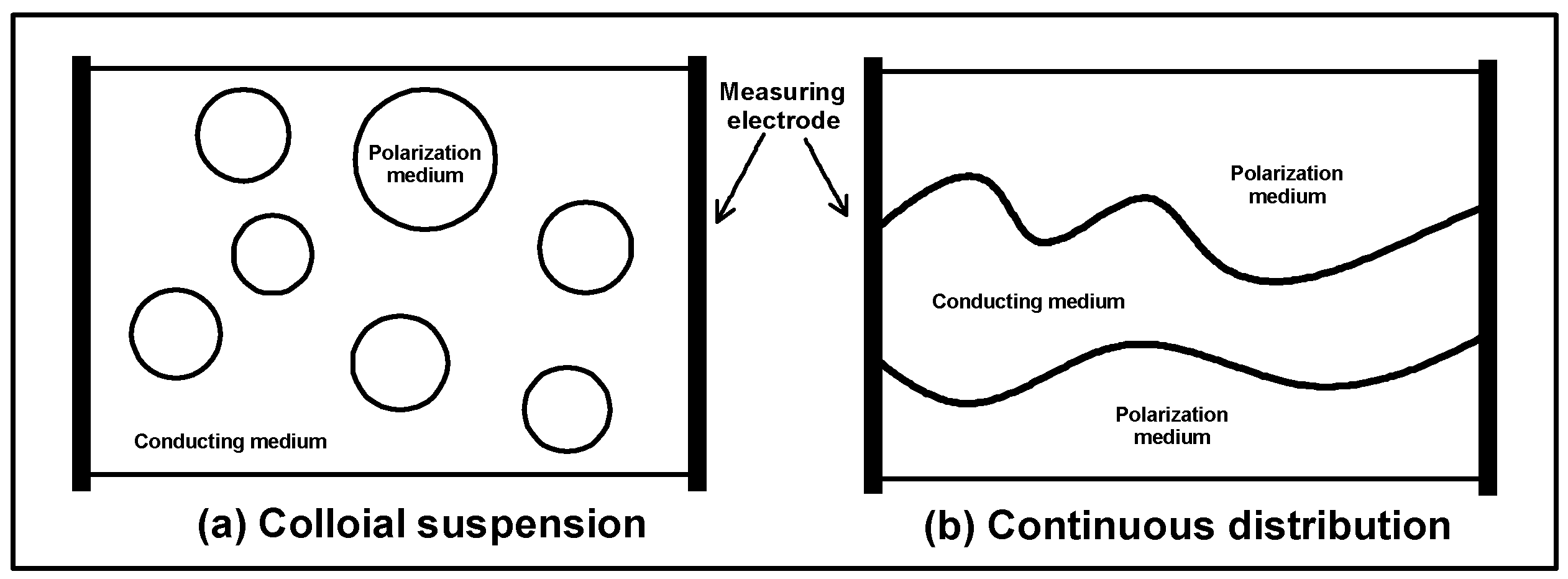
Revil and Cosenza [32] discussed the boundary polarization characteristics of the perturbed medium in actual rock under different distribution conditions. As shown in Figure 2, under (a) the colloidal suspension model meeting the assumptions of the MGEMTIP, the polarization medium provides complete polarization, including the boundary polarization of the Stern layer and the diffusion layer. Under (b) the continuous distribution model, the boundary polarization of the Stern layer and the diffusion layer is considered non-existent. But the reason for this process has not been explained by a definite theory.
In fact, the difference between the theoretical chargeability and the experimentally measured chargeability cannot be ignored. The strict modeling assumptions of the MGEMTIP for disturbance bodies (spherical disturbance bodies, infinite regions, etc.) do not apply to real rocks; the direct application of the MGEMTIP to the analysis of microscopic rocks is extremely risky. But the MGEMTIP provides an idea; we assume that all perturbed media are non-connected spheres (in this case, the polarization interface can establish a simple linear relationship with the volume of the perturbed media, so the polarization can also be determined by the volume of the perturbed media). However, the polarization interfaces of different perturbed media (low-resistivity minerals or pore fluids) in actual rocks deviate from the MGEMTIP to varying degrees. In the presence of multiple perturbation media, includes all potential perturbation media and considers them equally important, and highlights the perturbed media that conform to the MGEMTIP hypothesis (such as metallic minerals), so the difference between and highlights well-connected perturbation media (pore fluids or clay minerals).
Figure 2.
Different distribution types of perturbed medium. The rock is a combination of these two structures: (a) the worse the connectivity of the polarization medium, the higher the chargeability; (b) the higher the connectivity of the polarization medium, the lower the chargeability.
Figure 2.
Different distribution types of perturbed medium. The rock is a combination of these two structures: (a) the worse the connectivity of the polarization medium, the higher the chargeability; (b) the higher the connectivity of the polarization medium, the lower the chargeability.
The application results of the MGEMTIP in compacted reservoir rocks show that is always higher than . The relative difference between theoretical and measured chargeability has a strong positive correlation with permeability [30]. We analyze the reasons from the perspectives of formula derivation and experimental observation and summarize the main reasons for the difference between and :
- (a)
- Part of the boundary does not provide polarization. Since the finite volume of the actual rock sample is different from that in the open-domain model of the actual exploration object, the boundary formed by part of the perturbation is in direct contact with the insulating material (air or rubber sleeve) during the test process, and no complete boundary of the perturbation is provided. According to Appendix A, the chargeability difference between the infinite boundary MGEMTIP and the finite boundary MGEMTIP iswhere is the outer surface of the first perturbation, is the surface area of the first perturbation, is the ratio of the surface area and the outer surface, is the total volume of the rock, and the total surface area of all perturbations is determined by the size of the core, so in determining the volume of the perturbed medium, the bigger , the bigger will be.
- (b)
- By approximating the rock structure, the effective boundary decreases and the equivalent radius of perturbations increases. According to Appendix B, the difference between the chargeability of the MGEMTIP of the complex perturbations and the chargeability of the finite boundary MGEMTIP iswhere is the imaginary boundary area of the first perturbation, and the polarization difference is mainly caused by and . When there is a large-scale perturbation and the boundary is complex, the gets bigger.
According to (A8) in the Appendix B
where and are the time constants corresponding to the complex perturbation and the spherical perturbation, and is the proportion of the invalid boundary of the sphere approximating the complex perturbation. Compared with the time difference at the finite boundary of the MGEMTIP model, the time constant of the complex perturbation has an upward trend.
- (c)
- Limitation of the measured frequency band. According to the logarithmic form of the time constant in Formula (2)
The larger the perturbation medium in rock, the larger the time constant is. Micro-research such as the SDM model also has similar conclusions [15]. The measured chargeability obtained by the Debye decomposition algorithm is limited by the test frequency and does not include polarization far away from the frequency band. Therefore, the theoretical polarization corresponding to the large-scale perturbation cannot be measured. Although the Debye decomposition algorithm loses the polarization of some frequency bands in the discrete process [33], the measured chargeability is closer to the chargeability obtained in EM exploration and effectively reduces the influence of M-W polarization and test electrode polarization. At the same time, the DD algorithm, compared to the theoretical model, makes better use of the data.
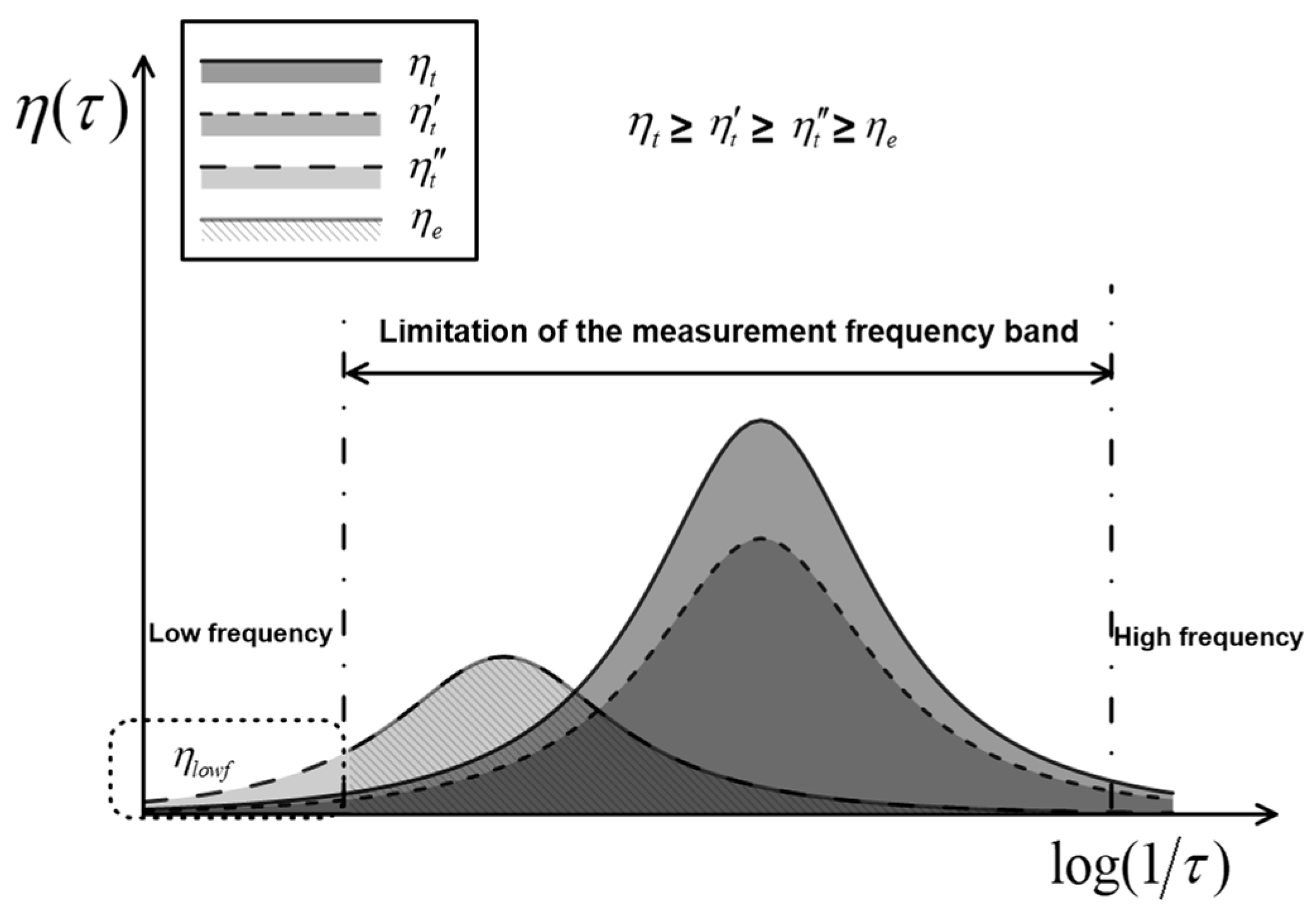
In summary, Figure 3 shows the schematic diagram of the MGEMTIP and the chargeability change with the corresponding time constant after considering various influencing factors. Thus, the theoretical chargeability and measured chargeability satisfy the following equation
According to the above analysis, the larger the equivalent scale of the perturbed medium in the rock, the bigger is. The perturbed medium interface in the actual rock is directly related to the scale of the pore fluid, whether the fluid is a perturbator or a background. Therefore, the larger the proportion of large-scale structures in the fluid-porous interface (in Figure 2, (b) structures in the rock are larger than (a) structures), the greater the difference between the theoretical chargeability and the measured chargeability is.
Figure 3.
The schematic diagram of the MGETIP and the chargeability change in the actual rock with the time constant under different conditions. The area enclosed by the chargeability (horizontal axis) corresponding to different time constants is the total chargeability. , , , and , respectively, indicate the chargeability of the MGEMTIP model, the chargeability of the finite boundary model, the chargeability of the finite boundary complex structure model, and the measured chargeability. In the low-frequency band outside the actual measurement frequency band, the chargeability corresponding to large-scale structure still exists.
2.3. Permeability Prediction Model
Based on MGEMTIP, the statistical correlation between theoretical and measured porosity and permeability is analyzed [30]. Combined with the characteristics of low-resistivity media (clay and secondary metals) in low porosity and permeability reservoirs, we believe that the difference between the measured chargeability of the rock and the theoretical chargeability based on the MGEMTIP can be used to evaluate the permeability of low-porosity and permeability rocks with conductive minerals and have proposed a semi-empirical permeability prediction model (-prediction model)
where and , respectively, correspond to the theoretical chargeability and measured chargeability of the measured rock, and is the rock characteristic index. According to theoretical analysis, . The characteristic index of the studied reservoir is obtained by experimental fitting of reservoir samples. When the measured chargeability is close to the theoretical chargeability, , the permeability is , and the rock is close to the theoretical state without the hypothesis of connectivity; when the measured chargeability is extremely small, , the rock permeability is , and the rock is close to the limiting state of full connectivity (no polarization).
2.4. Applicability Analysis of the Permeability Prediction Model
The experiment was carried out with a high salinity solution, mainly for the following reasons: (a) By saturating high-concentration electrolyte solution (NaCl > 0.5 mol/L), saturated rocks can effectively reduce the polarization intensity of the diffusion layer [34], which in turn highlights the polarization caused by the perturbed medium boundary. The MGEMTIP ignores the diffusion layer polarization, and the test rock saturated with a high salinity solution is more consistent with the MGEMTIP hypothesis. (b) According to the deep reservoirs studied, the salinity of the high-salinity solution is closer to that of groundwater.
Analysis of the model error in the prediction model (7) shows that the theoretical chargeability and measuring chargeability may have calculation or estimation errors. Let us consider the relative error relationship corresponding to the model
where and correspond to the absolute error between the measured and estimated chargeability and the actual chargeability. Under the condition that the error is fixed, the error will be increased to . According to the above analysis, low-porosity and low-permeability rocks containing low-resistivity minerals are suitable for Formula (7).
Theoretically, high-porosity and high-permeability rocks are not suitable for this prediction model. The high-porosity and permeability rocks do not conform to the small perturbation body assumption of the MGEMTIP model. When is extremely small, the measurement accuracy also easily affects the prediction results. However, this prediction model still has a certain ability to predict high-porosity and permeability rocks. Using pure sandstone as an example, with high-resistivity quartz minerals as the main conductive medium and pore fluid as the main polarization medium (although the pore fluid of the actual rock is only a conductive medium, the main polarization medium in MGEMTIP must be a low-resistivity medium), this prediction model will have a theoretical relationship with other electrical permeability prediction models, as we will explain further in the Discussion section.
3. Physics Experiment
3.1. Experimental Sample Information
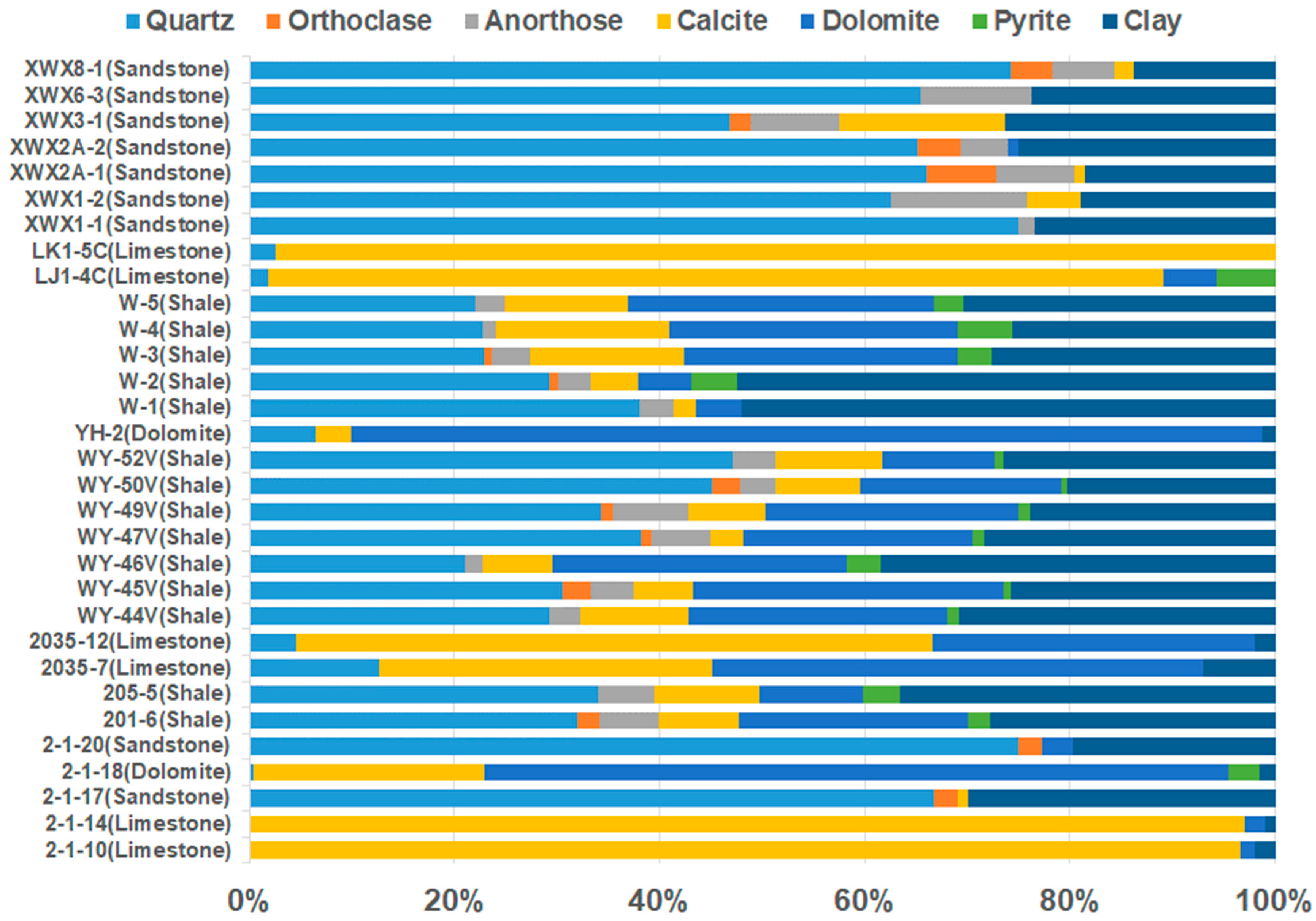
The shale reservoir rocks in southern China are rich in metallic minerals and low in porosity and permeability, which meet the applicable requirements of the prediction model. We selected two sets of high-clay rocks (with a clay content above 15%) and low-clay rocks (with a clay content less than 5%) for experiments. The high-clay rocks included shale and sandstone, and the low-clay rocks included sandstone, limestone, and dolomite. One set of samples is used to fit the model parameters, and the other set is used only for prediction. The clay content affects the main conducting medium of the equivalent medium, so we fit them separately. The rock structure and conducting mineral composition information are shown in Table 1. The fitted high-clay rocks include 11 reservoir samples with a small range of permeability (0.01 mD–1 mD) due to high clay content. The fitted low-clay rocks include 6 reservoir samples and 3 high-permeability artificial sandstones with a wide range of permeabilities (0.01 mD–1000 mD). Fractures along the bedding direction were generated in part of the shale during the saturation process. When the measured direction is parallel to the fracture direction, permeability is abnormally high (such as W4). However, since this structure is a case of theoretical analysis in Figure 2b, it was not removed as an abnormal sample. The predicted high-clay rocks include 12 reservoir samples, and the predicted low-clay rocks include 1 reservoir sample and 3 high-permeability artificial sandstones with a wide range of permeability (0.001 mD–1000 mD). The results of dry resistivity measurements (resistivity amplitude measured after drying at 80 °C for 24 h, at 1 Hz) show that high-component clay forms a conductive channel with better conductivity in the rock and has a lower dry resistivity. Figure 4 is a diagram of the rock composition. The experiment mainly focuses on the high-conductivity minerals in the rock, mainly the content of clay and pyrite. High-resistivity minerals (HRM) are considered to provide no electrical conductivity, while artificial sandstone has no low-resistivity components.
We tested 36 rock samples for the CR, porosity, and permeability at a pressure of 10 MPa and a temperature of 40 °C, these samples are cylinders 1 inch in diameter and 4~5 cm long. The test frequency range is 10−2 ~104 Hz, saturated with 4% NaCl electrolyte solution, and the solution resistivity is 0.114 ohm-m under the test environment.
Figure 4.
Sample mineral compositions. Pyrite and clay have high electrical conductivity, which has a significant impact on the electrical polarization or electrical conductivity of the rock.
Figure 4.
Sample mineral compositions. Pyrite and clay have high electrical conductivity, which has a significant impact on the electrical polarization or electrical conductivity of the rock.

Table 1.
Physical property information of rock samples.
| No. | Lithology | Porosity/% | Permeability | Dry Resistivity | Conductive Mineral | Experimental Project | |
|---|---|---|---|---|---|---|---|
| /mD | /ohm-m | Clay/% | Pyrite/% | ||||
| 2-1-17 | Sandstone | 3.50 | 0.0230 | 5.70 × 10² | 30 | 0 | Fitting samples with high clay |
| 2-1-20 | Sandstone | 2.20 | 0.0750 | 2.50 × 10³ | 19.7 | 0 | |
| 201-6 | Shale | 5.40 | 0.4850 | 5.90 × 10² | 27.8 | 2.2 | |
| 205-5 | Shale | 5.90 | 0.3810 | 9.40 × 10² | 36.5 | 3.7 | |
| WY-44V | Shale | 3.80 | 0.0400 | 8.50 × 10² | 30.8 | 0.9 | |
| WY-45V | Shale | 1.50 | 0.0350 | 8.30 × 10³ | 25.7 | 0.8 | |
| WY-46V | Shale | 2.10 | 0.0300 | 7.80 × 10² | 38.5 | 3.1 | |
| WY-47V | Shale | 1.30 | 0.0500 | 1.00 × 10⁴ | 28.4 | 0.8 | |
| WY-49V | Shale | 1.20 | 0.0580 | 2.30 × 10⁴ | 23.9 | 1 | |
| WY-50V | Shale | 1.00 | 0.0660 | 3.40 × 10⁴ | 20.3 | 0.8 | |
| WY-52V | Shale | 2.40 | 0.0270 | 1.10 × 10³ | 26.5 | 0.7 | |
| 2-1-10 | Limestone | 0.33 | 0.0420 | 3.10 × 10⁶ | 2 | 0 | Fitting samples with low clay |
| 2-1-14 | Limestone | 0.57 | 0.0300 | 1.40 × 10⁶ | 1 | 0 | |
| 2-1-18 | Dolomite | 1.40 | 0.1100 | 1.30 × 10⁶ | 1.5 | 3.1 | |
| 2035-7 | Limestone | 4.00 | 0.5440 | 7.30 × 10³ | 7 | 0 | |
| 2035-12 | Limestone | 5.40 | 0.1180 | 2.30 × 10⁷ | 2 | 0 | |
| YH-2 | Dolomite | 2.97 | 1.2100 | 2.20 × 10⁵ | 1.3 | ||
| AS-2 | Sandstone | 7.75 | 3.4500 | 8.16 × 10⁶ | 0 | 0 | |
| AS-4 | Sandstone | 12.84 | 87.5000 | 1.08 × 10⁷ | 0 | 0 | |
| AS-5 | Sandstone | 18.36 | 326.0000 | 1.11 × 10⁷ | 0 | 0 | |
| W1 | Shale | 4.84 | 0.1100 | 1.80 × 10³ | 52 | 0 | Predicted samples with high clay |
| W2 | Shale | 5.42 | 0.3160 | 1.28 × 10³ | 52.4 | 4.5 | |
| W3 | Shale | 5.26 | 0.6260 | 3.61 × 10³ | 27.6 | 3.4 | |
| W4 | Shale | 4.36 | 3.9900 | 2.24 × 10³ | 25.6 | 5.4 | |
| W5 | Shale | 4.21 | 0.1310 | 4.39 × 10³ | 30.3 | 2.9 | |
| XWX1-1 | Sandstone | 9.93 | 0.8019 | 4.23 × 10² | 23.5 | 0 | |
| XWX1-2 | Sandstone | 2.22 | 0.0712 | 1.26 × 10⁴ | 19 | 0 | |
| XWX2A-1 | Sandstone | 7.88 | 0.2643 | 1.44 × 10⁴ | 18.6 | 2.3 | |
| XWX2A-2 | Sandstone | 5.53 | 0.3578 | 4.22 × 10² | 25 | 0 | |
| XWX3-1 | Sandstone | 0.86 | 0.0045 | 9.91 × 10⁴ | 26.3 | 0 | |
| XWX6-3 | Sandstone | 6.72 | 0.8354 | 8.31 × 10² | 23.7 | 0 | |
| XWX8-1 | Sandstone | 8.74 | 0.9193 | 1.45 × 10⁴ | 13.8 | 0 | |
| LJ1-4C | Limestone | 0.18 | 0.0010 | 1.36 × 10⁵ | 0 | 5.7 | Predicted samples with low clay |
| AS-6 | Sandstone | 15.80 | 247.0000 | 9.57 × 10⁶ | 0 | 0 | |
| AS-7 | Sandstone | 16.50 | 331.4000 | 1.25 × 10⁷ | 0 | 0 | |
| AS-8 | Sandstone | 9.70 | 12.6000 | 7.64 × 10⁶ | 0 | 0 | |
3.2. Theoretical Chargeability and Measured Chargeability
The estimation of the theoretical chargeability requires an equivalent medium conforming to the MGEMTIP model. In actual rocks, the construction of an equivalent medium needs to determine the spatial relationship between various conductive minerals and pore fluids, combined with mineral components, and comprehensively realized by scanning electron microscopy (SEM). Mineral composition analysis, dry resistivity testing, and scanning electron microscopy are effective means to accurately construct an equivalent medium.
According to the model relationship of , the construction method of the equivalent medium is relatively rough. The conductive medium and the polarized medium in the rock minerals are selected (proving that the conductivity of polarized media is much higher than that of conductive media), and the spatial relationship between the two media is analyzed in combination with different lithologies
where is the relative volume fraction as follows
where is the conductive medium, is the perturbed medium, and is the spatial correlation function between the two media. Figure 5 shows the spatial relationship between clay minerals and pyrite particles. Clay in the shale and the secondary pyrite satisfy the , and the other conductive media and perturbed media are assumed to be spatially uncorrelated, and satisfy the .
The measured chargeability is analyzed through experimental data, and the theoretical chargeability is estimated based on the MGEMTIP and rock composition. The saturated rock test and analysis results are shown in Table 2. Saturation resistivity and are obtained by the Debye decomposition method [35].
When constructing the equivalent medium, we distinguish between low-clay rocks and high-clay rocks. We choose clay as the main conductive medium for high-clay rocks and select high-resistivity minerals as the main conductive medium for low-clay rocks. Further fitting and prediction are also based on these two different equivalent media.
For low-clay rocks with high porosity and permeability, this equivalence relationship is unreasonable (solution is more likely to be the dominant conducting medium), but therefore the difference between and is also larger, indicating that these rocks have greater permeability. When the porosity is greater than 22.3%, will exceed 1. There is a theoretical relationship between the in the MGMETIP model and the chargeability in the Cole-Cole
Only in terms of formula, when the is small, the difference between and is not large; even if exceed 1, will not exceeds 1. So formally, the establishment of the Formula (9) is still feasible.
4. Results and Discussion
4.1. Fitting Relationship
Fitting and predictive analysis were performed based on 36 samples in the experiment. Figure 6 shows the relationship between measured permeability and the relative chargeability difference of rock samples. The relative chargeability difference is calculated according to Table 2. From a larger data range, although the fitting degree is reduced ( for 6 samples in Tong et al. [30]), the positive correlation between the relative polarizability difference and the measured permeability still exists. The data distribution also indicates that Formula (7) has a better fitting relationship. Compared with the relative chargeability difference , Formula (7) adds 1 degree of freedom, which can better match the data relationship. We also compare Formula (7) with the two electrical K-C relationships used in [19], and having the same degree of freedom allows us to better compare the fitting and prediction effects.
The two electrical K-C relationships are
and
where a, b, c is the fitting parameter, respectively, correspond to the rock formation factor, the imaginary part of the low-frequency (1 Hz) conductivity, and the normalized chargeability, where and . The IP parameters required by the model are shown in Table 3.
The objective functions used in the fitting of the three predictive permeability models are
where is the measured permeability, is the theoretical permeability, and N is the total number of samples. The coefficient of determination and geometric mean error D are
and
Figure 7 shows the fitting results of all experimental samples by three prediction models, indicating that the three methods have little difference in fitting the overall data (). The overall fit cannot show the difference between the three prediction models. Fitting some samples and predicting other samples can better highlight the differences in the prediction models.
4.2. Prediction Results
According to the construction of the equivalent medium of the MGEMTIP model, the predicted rocks are divided into high-clay and low-clay samples, and three model fitting formulas are used to predict and analyze the high-clay and low-clay predicted samples. Table 4 and Figure 8 are the prediction model and the prediction result.
Table 4 shows that the -prediction model has the best coefficient of determination () for high-clay samples and the worst coefficient of determination () for low-clay samples. The permeability range of high-clay samples is relatively narrow, and the coefficient of determination is relatively low. Consistent with the theoretical analysis, the low-clay samples containing a large number of high-permeability samples are too different from the constructed equivalent medium, and the MGEMTIP’s applicability is limited.
Figure 8 indicates that the -prediction results are the best for high-clay samples, regardless of whether the model is based on high-clay samples () or low-clay samples (). The -prediction has limited applicability to low-clay samples, especially high-permeability samples.
- prediction results show that the prediction of high clay samples has obvious deviations and is generally high. The high clay content reduces the formation factor F, but the imaginary part of the low-frequency (1 Hz) conductivity does not reflect the clay polarization (the clay particles are smaller, and the frequency of polarization is higher). In contrast, the deviations of the -prediction for high clay samples are small, even in prediction models based on low clay samples. While high clay reduces F, also increases due to the polarization formed by the clay ( can be seen as the average of over a frequency band). The effects of clay on conduction and polarization cancel each other out, making -prediction more effective.
From the prediction results, the -prediction model is more beneficial to eliminate the influence of low-resistivity minerals (clay or metal minerals) on the permeability prediction. However, the model is easy to be distort when predicting high porosity and permeability samples, so the prediction model based on MGEMTIP is more suitable for low porosity and permeability reservoirs.
4.3. Relationship with K-C Model
The main polarization medium is a pore solution, and low-resistivity minerals are in the - prediction model for low-clay samples. If the rock does not contain low-resistivity minerals, the model has a certain theoretical relationship with the K-C model. The K-C model based on the capillary model is
where is the porosity of the rock, r is the equivalent pore radius, is the form factor, and T is the pore tortuosity. When the rock uses pore fluid as the main polarization medium, and the high permeability rocks that satisfies , Formula (7) combined with Formula (9) satisfy
where is the surface area per unit pore volume. A large number of studies have shown that and have positive correlation [12,13,14], and in the capillary model (h is the capillary length). The pore structure that causes polarization usually does not satisfy the capillary assumption. can be regarded as a correction to , reducing the influence of the pore structure that causes polarization.
4.4. Application of the Permeability Prediction Model
The -prediction model based on the MGEMTIP has a certain locality, and the collection of geophysical logging data and the laboratory core test of the reservoir area are essential to constructing an effective equivalent medium. Compared with the two electrical K-C models, the -prediction model has certain advantages in the prediction of low porosity and low permeability reservoirs because it fully understands the structural characteristics of reservoir rocks in the investigated area. EM exploration alone cannot effectively translate electrical parameters into reservoir physical properties. Combining geological lithology, seismic stratification, and logging data, the equivalent medium structure of the survey area was constructed to obtain the theoretical chargeability . Combined with logging saturation and experimental study correction, the exploration data provides measured chargeability of the survey area in saturated brine. The characteristic index a, b, c can be obtained from the experimental data of the survey area. Substituting a, b, c, , and into the prediction formula allows the permeability of the surveyed area to be calculated. Both experiment and theory are carried out for rocks with saturated brine, and the IP characteristics of samples with unsaturated brine have not been analyzed, which makes it difficult to correct actual unsaturated strata and limits the application of this method. However, the -prediction model is still suitable for research areas with high brine saturation. In fact, the -prediction model has some potential for deep geothermal fracturing monitoring or enhanced oil recovery engineering.
5. Conclusions
The chargeability based on the MGEMTIP is different from the measured chargeability in the reservoir rock. The main reasons for the difference in chargeability are the limitation of measurement frequency and the structural deviation between the model hypothesis and the reservoir rock. Based on the positive correlation between the chargeability difference and the measured permeability, the -prediction model based on MGEMTIP is proposed.
The applicability of the -prediction model is analyzed theoretically and experimentally. Theoretical analysis shows that although the -prediction has a theoretical correlation with the K-C model, the -prediction is not suitable for high porosity and high permeability rock permeability prediction due to the failure of the equivalent medium theory. Experimentally, both the fitting and prediction results show that, compared with the two electrical K-C models, the -prediction model is suitable for low porosity and permeability rocks containing low-resistivity minerals, and the prediction results can be effectively constrained within the same order of magnitude (D < 1).
The -prediction model is a semi-quantitative relationship between rock permeability and chargeability that depends on accurate modeling of the rock equivalent medium. The applicability of this prediction model to actual reservoirs is still being explored. The -prediction model combining geological, seismic, and logging data is beneficial to reservoir permeability prediction based on EM exploration and has certain application potential in geothermal fracturing monitoring and enhanced oil recovery engineering.
Author Contributions
Conceptualization, L.Y.; Methodology, X.T.; Validation, X.T.; Investigation, K.X.; Data curation, K.X.; Writing—original draft, X.T.; Writing—review & editing, L.Y.; Project administration, L.Y.; Funding acquisition, X.T., L.Y. and K.X. All authors have read and agreed to the published version of the manuscript.
Funding
This research was funded by the National Natural Science Foundation of China (NSFC), grant numbers 42204079, 42030805, and 42174083.
Data Availability Statement
The data used to support the findings of this study are available from the corresponding author upon request.
Conflicts of Interest
The authors declare no conflict of interest.
Appendix A
In the equivalent medium model established according to Figure A1, the equivalent conductivity is [30]
where is the background conductivity, and correspond to the structure tensor and background volume of the background medium, and correspond to the structure tensor and surface structure tensor of the perturbed volume numbered , , and correspond to the effective surface area and volume of the perturbation numbered l, , and are the spatial average and the surface normal average, respectively.
The space of the rock sample in the laboratory, unlike exploration, is limited, and the outer boundary area cannot be ignored compared with the inner boundary area. Therefore, it is necessary to consider that part of the perturbation boundary is at the outer boundary and will form the outer boundary of the rock by contact with air or rubber bands and other high-resistivity bodies during the test. For any perturbation , its boundary area consists of an inner boundary and an outer boundary, formulated as . When its outer boundary conditions contact the high-resistivity medium and the corresponding boundary conditions satisfy , then,
When it is substituted in the one-dimensional model, the equivalent conductivity of the finite-space medium is obtained
where is the background resistivity and , , , and are the conductivity, composition, interface chargeability factor, and radius of the perturbation numbered , respectively. With substituted parameters, the formula is converted into the resistivity in the Cole-Cole model
The chargeability is
where ; in case of small volume disturbance, . The time constant is consistent with that in the unbounded MGEMTIP model.
Appendix B
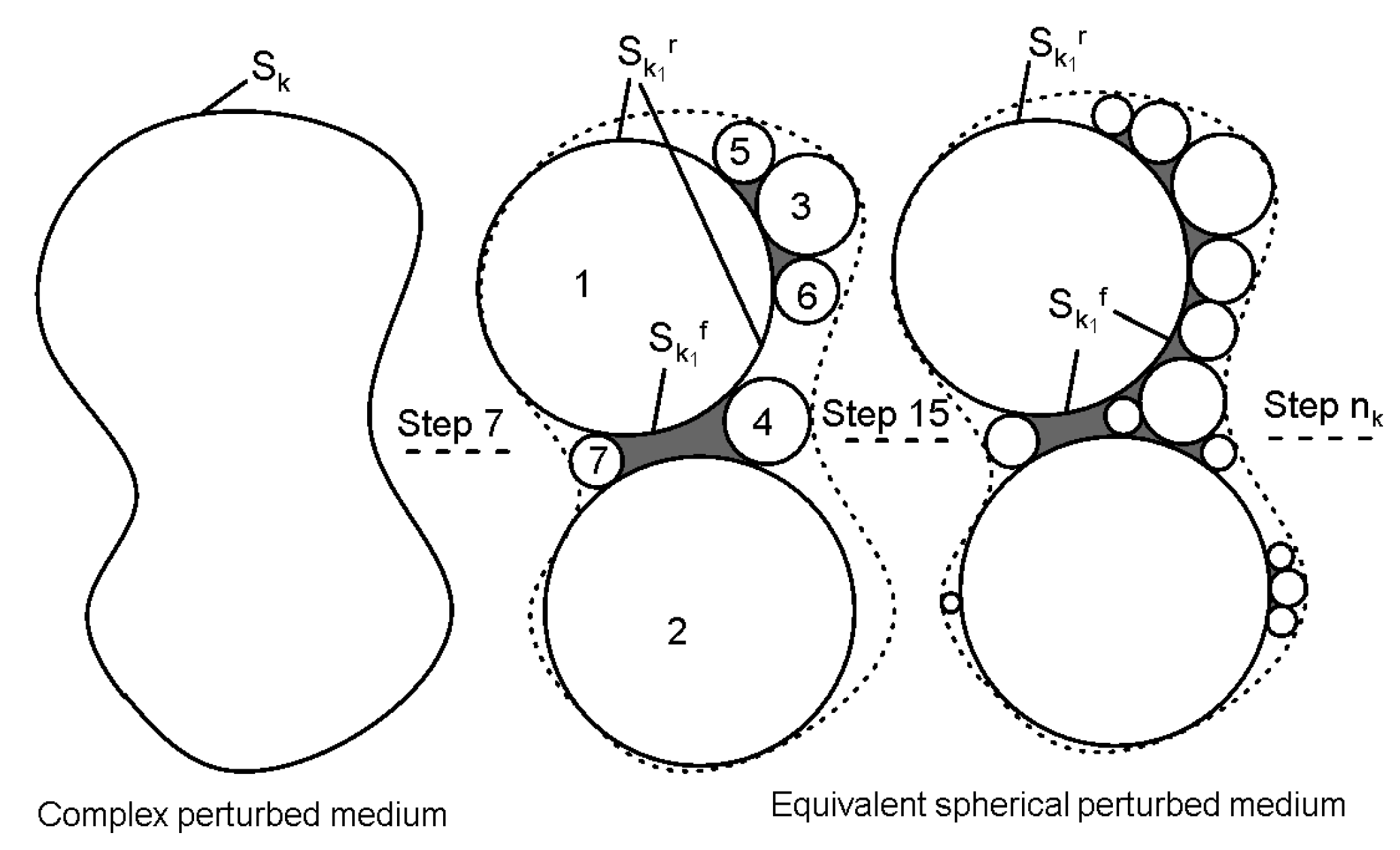
For the effective electrical properties of real rocks, we considered the existence of non-spherical perturbed media . For the applicability of the MGEMTIP model, a series of sphere models (, correspond to all perturbed media that satisfy , which is the number of perturbed spheres of the overall model) need to be used to approximate the non-spherical model. The approximation steps are shown in F-1. At every step, a sphere is added (satisfying ), gradually approximating the structure of the perturbed medium from the interior of the perturbation. Since the rock structure is not infinitely small, it is considered that at the step numbered , the total volume is . The total boundary of spheres increases as the number of spheres increases, and at the step numbered , all sphere boundaries are divided into real boundaries and imaginary boundaries . The true boundary is , formulated as . Different from the boundary conditions of finite space, the imaginary boundary not only satisfies the change of boundary conditions , but also affects the calculation of the surface area of the perturbation.
Figure A1.
A step diagram of a spherical perturbed medium approximating a complex perturbed medium.
For any sphere of the perturbed medium k at the step numbered of the MGEMTIP model, the effective area is , which is less than the surface area of the sphere . When the perturbation is a sphere, the equivalent radius in Formula (A3) can be expressed as . When we substitute the complex perturbation in the finite boundary medium, the equivalent conductivity is
With substituted parameters, the formula is converted to the resistivity form in the Cole-Cole model
Then, the chargeability is
where . In case of small volume disturbance, .
The time constant is obtained as follows
References
- Zhang, R.; Yan, L.; Sun, S.; Jiang, X.; Xie, X.; Jin, G. IP parameter extraction from TFEM data in the time domain. Oil Geophys. Prospect. 2016, 51, 1227–1232. [Google Scholar]
- Feng, L.; Li, Q.; Cameron, S.D.; He, K.; Colby, R.; Walker, K.M.; Deckman, H.W.; Ertaş, D. Quantifying induced polarization of conductive inclusions in porous media and implications for geophysical measurements. Sci. Rep. 2020, 10, 1669. [Google Scholar] [CrossRef] [PubMed] [Green Version]
- Revil, A.; Vaudelet, P.; Su, Z.; Chen, R. Induced Polarization as a Tool to Assess Mineral Deposits: A Review. Minerals 2022, 12, 571. [Google Scholar] [CrossRef]
- Linde, N.; Chen, J.; Kowalsky, M.B.; Hubbard, S. Applied Hydrogeophysics; Springer: Berlin/Heidelberg, Germany, 2006; pp. 9–44. [Google Scholar]
- Slater, L. Near surface electrical characterization of hydraulic conductivity: From petrophysical properties to aquifer geometries—A review. Surv. Geophys. 2007, 28, 169–197. [Google Scholar] [CrossRef]
- Revil, A.; Eppehimer, J.; Skold, M.; Karaoulis, M.; Godinez, L.; Prasad, M. Low-frequency complex conductivity of sandy and clayey materials. J. Colloid Interface Sci. 2013, 398, 193–209. [Google Scholar] [CrossRef] [PubMed]
- Kozeny, J. Uber kapillare leitung der wasser in boden. R. Acad. Sci. Vienna Proc. Class I 1927, 136, 271–306. [Google Scholar]
- Guéguen, Y.; Palciauskas, V. Introduction to the Physics of Rocks; Princeton University Press: Princeton, NJ, USA, 1994. [Google Scholar]
- Katz, A.; Thompson, A. Quantitative prediction of permeability in porous rock. Phys. Rev. B 1986, 34, 8179. [Google Scholar] [CrossRef]
- Kostek, S.; Schwartz, L.M.; Johnson, D.L. Fluid permeability in porous media: Comparison of electrical estimates with hydrodynamical calculations. Phys. Rev. B 1992, 45, 186. [Google Scholar] [CrossRef]
- Vinegar, H.J.; Waxman, M.H. Induced polarization of shaly sands. Geophysics 1984, 49, 1267–1287. [Google Scholar] [CrossRef]
- de Lima, O.A. Water saturation and permeability from resistivity, dielectric, and porosity Logs. Geophysics 1995, 60, 1756–1764. [Google Scholar] [CrossRef]
- Börner, F.; Schopper, J.; Weller, A. Evaluation of transport and storage properties in the soil and groundwater zone from induced polarization measurements1. Geophys. Prospect. 1996, 44, 583–601. [Google Scholar] [CrossRef]
- Weller, A.; Slater, L. Permeability estimation from induced polarization: An evaluation of geophysical length scales using an effective hydraulic radius concept. Near Surface Geophys. 2019, 17, 581–594. [Google Scholar] [CrossRef] [Green Version]
- Schwarz, G. A theory of the low-frequency dielectric dispersion of colloidal particles in electrolyte solution1,2. J. Phys. Chem. 1962, 66, 2636–2642. [Google Scholar] [CrossRef]
- Revil, A.; Florsch, N. Determination of permeability from spectral induced polarization in granular media. Geophys. J. Int. 2010, 181, 1480–1498. [Google Scholar] [CrossRef]
- Binley, A.; Slater, L.D.; Fukes, M.; Cassiani, G. Relationship between spectral induced polarization and hydraulic properties of saturated and unsaturated sandstone. Water Resour. Res. 2005, 41, 1–13. [Google Scholar]
- Tong, M.; Li, L.; Wang, W.; Jiang, Y. Determining capillary-pressure curve, pore-size distribution, and permeability from induced polarization of shaley sand. Geophysics 2006, 71, N33–N40. [Google Scholar] [CrossRef]
- Weller, A.; Slater, L.; Binley, A.; Nordsiek, S.; Xu, S. Permeability prediction based on induced polarization: Insights from measurements on sandstone and unconsolidated samples spanning a wide permeability range. Geophysics 2015, 80, D161–D173. [Google Scholar] [CrossRef]
- Fiandaca, G.; Maurya, P.; Balbarini, N.; Hördt, A.; Christiansen, A.; Foged, N.; Bjerg, P.L.; Auken, E. Permeability estimation directly from logging-while-drilling induced polarization data. Water Resour. Res. 2018, 54, 2851–2870. [Google Scholar] [CrossRef] [Green Version]
- Maurya, P.K.; Balbarini, N.; Møller, I.; Rønde, V.; Christiansen, A.; Bjerg, P.L.; Auken, E.; Fiandaca, G. Subsurface imaging of water electrical conductivity, hydraulic permeability and lithology at contaminated sites by induced polarization. Geophys. J. Int. 2018, 213, 770–785. [Google Scholar] [CrossRef] [Green Version]
- Ghanbarian, B.; Javadpour, F. Upscaling pore pressure-dependent gas permeability in shales. J. Geophys. Res. Solid Earth 2017, 122, 2541–2552. [Google Scholar] [CrossRef]
- Revil, A.; Binley, A.; Mejus, L.; Kessouri, P. Predicting permeability from the characteristic relaxation time and intrinsic formation factor of complex conductivity spectra. Water Resour. Res. 2015, 51, 6672–6700. [Google Scholar] [CrossRef] [Green Version]
- Revil, A.; Leroy, P. Constitutive equations for ionic transport in porous shales. J. Geophys. Res. Solid Earth 2004, 109, 1–19. [Google Scholar] [CrossRef]
- Weller, A.; Zhang, Z.; Slater, L. High-salinity polarization of sandstones. Geophysics 2015, 80, D309–D318. [Google Scholar] [CrossRef]
- Revil, A.; Florsch, N.; Mao, D. Induced polarization response of porous media with metallic particles—Part 1: A theory for disseminated semiconductors. Geophysics 2015, 80, D525–D538. [Google Scholar] [CrossRef]
- Wong, J. An electrochemical model of the induced-polarization phenomenon in disseminated sulfide ores. Geophysics 1979, 44, 1245–1265. [Google Scholar] [CrossRef]
- Zhdanov, M. Generalized effective-medium theory of induced polarization. Geophysics 2008, 73, F197–F211. [Google Scholar] [CrossRef]
- Lin, W.; Zhdanov, M.S.; Burtman, V.; Gribenko, A. GEMTIP inversion of complex resistivity data using a hybrid method based on a genetic algorithm with simulated annealing and regularized conjugate gradient method. In SEG Technical Program Expanded Abstracts 2015; Society of Exploration Geophysicists: Tulsa, OK, USA, 2015; pp. 952–956. [Google Scholar]
- Tong, X.; Yan, L.; Xiang, K. Modifying the Generalized Effective-medium Theory of Induced Polarization Model in Compacted Rocks. Geophysics 2020, 85, 1–44. [Google Scholar]
- Latt, K.M.; Giao, P. Prediction of permeability of cement-admixed soft clay using resistivity and time-domain IP measurements. J. Appl. Geophys. 2017, 137, 92–103. [Google Scholar] [CrossRef]
- Revil, A.; Cosenza, P. Comment on “Generalized effective-medium theory of induced polarization”. Geophysics 2010, 75, X7–X9. [Google Scholar] [CrossRef]
- Weigand, M.; Kemna, A. Relationship between Cole–Cole model parameters and spectral decomposition parameters derived from SIP data. Geophys. J. Int. 2016, 205, 1414–1419. [Google Scholar] [CrossRef]
- Revil, A. Ionic diffusivity, electrical conductivity, membrane and thermoelectric potentials in colloids and granular porous media: A unified model. J. Colloid Interface Sci. 1999, 212, 503–522. [Google Scholar] [CrossRef] [PubMed]
- Nordsiek, S.; Weller, A. A new approach to fitting induced-polarization spectra. Geophysics 2008, 73, F235–F245. [Google Scholar] [CrossRef]
Figure 1.
The schematic diagram of the effective medium theory. A heterogeneous medium contains many different types of perturbed media, each of which contains resistivity , effective radius , and surface-polarizability coefficient . The resistivity of a heterogeneous medium is equivalent to the CR of an effective medium through the effective-medium approach.
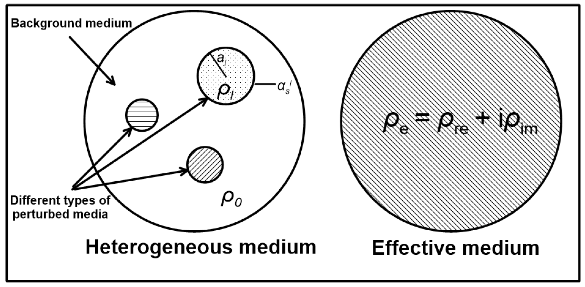
Figure 5.
SEM of reservoir shale. The secondary pyrite particles in clay minerals are aggregated, and the particles as a whole are about 0.01 mm in scale.
Figure 5.
SEM of reservoir shale. The secondary pyrite particles in clay minerals are aggregated, and the particles as a whole are about 0.01 mm in scale.
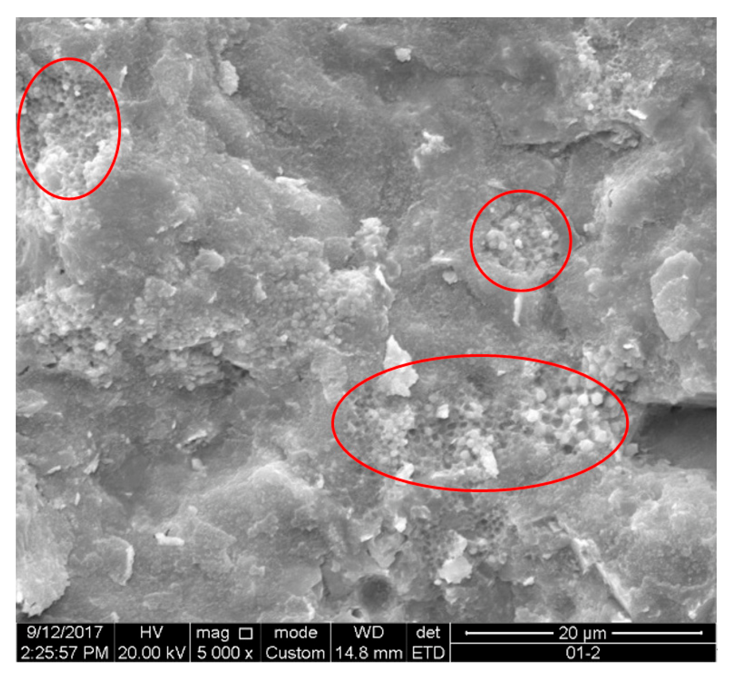
Figure 6.
Relationship between measured permeability and relative chargeability difference of rock samples. The samples include 30 new samples and 6 samples from Tong et al. [30].
Figure 6.
Relationship between measured permeability and relative chargeability difference of rock samples. The samples include 30 new samples and 6 samples from Tong et al. [30].

Figure 7.
Fitting results from three prediction models for 36 samples. The difference of R2 is smaller.
Figure 7.
Fitting results from three prediction models for 36 samples. The difference of R2 is smaller.
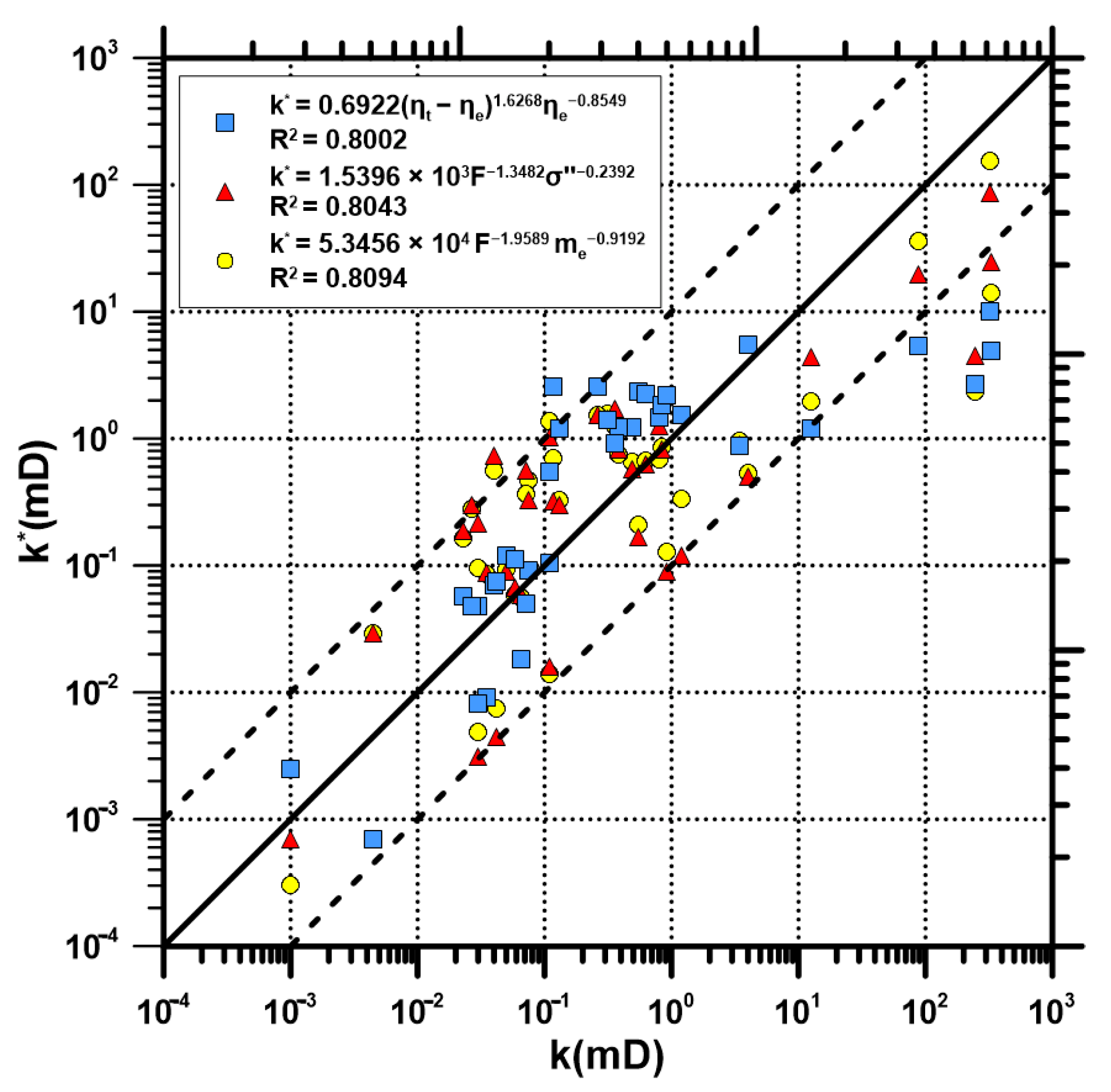
Figure 8.
Prediction results of three models based on (a) high-clay predicted samples and (b) low-clay predicted samples; (a) the three prediction models based on high clay rocks have poor prediction results for low clay rocks (D > 1), while the -prediction for high clay samples is best ( ); (b) the -prediction model based on low clay rocks has a worst prediction result for low clay rocks ( ) and a best prediction result for high clay rocks ( ).
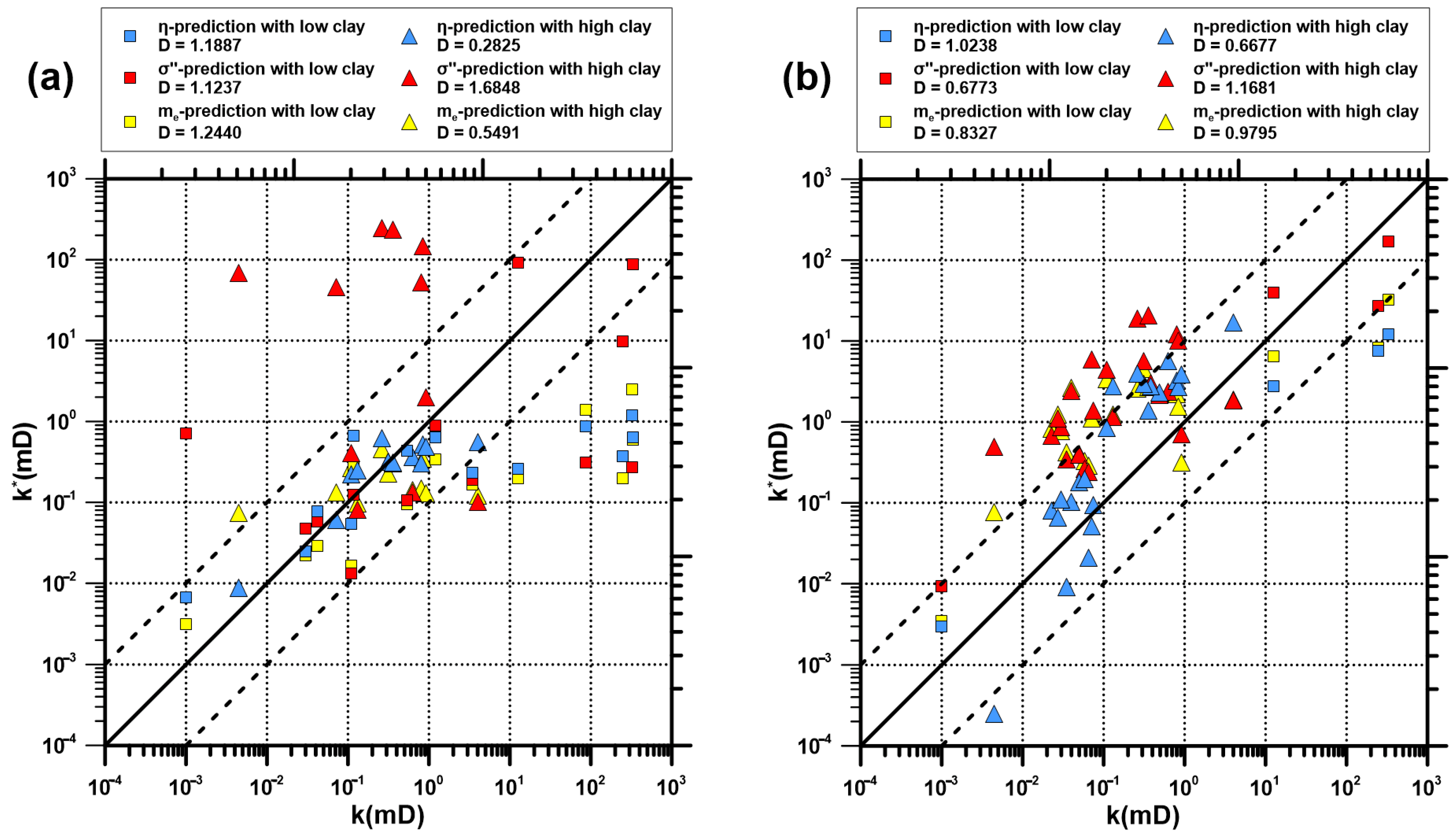
Table 2.
Rock test and analysis results.
| No. | Main Conductive Medium | Main Polarization Medium | Spatial Correlation | |||||
|---|---|---|---|---|---|---|---|---|
| Medium | Medium | |||||||
| 2-1-17 | 66.42 | 9.49% | Clay | 28.95% | Solution | 3.50% | 0 | 15.75% |
| 2-1-20 | 44.02 | 4.37% | Clay | 19.27% | Solution | 2.20% | 0 | 9.90% |
| 201-6 | 25.79 | 5.33% | Clay | 26.30% | Pyrite | 2.08% | 1 | 35.61% |
| 205-5 | 19.24 | 7.20% | Clay | 36.50% | Pyrite | 3.48% | 1 | 42.93% |
| WY-44V | 20.37 | 10.22% | Clay | 29.63% | Pyrite | 1.15% | 1 | 17.53% |
| WY-45V | 132.24 | 10.15% | Clay | 25.31% | Pyrite | 0.69% | 1 | 12.26% |
| WY-46V | 69.52 | 28.61% | Clay | 37.69% | Pyrite | 3.23% | 1 | 38.57% |
| WY-47V | 138.89 | 8.23% | Clay | 28.03% | Pyrite | 1.09% | 1 | 17.43% |
| WY-49V | 168.93 | 11.95% | Clay | 23.61% | Pyrite | 1.19% | 1 | 22.59% |
| WY-50V | 194.76 | 10.08% | Clay | 20.10% | Pyrite | 0.59% | 1 | 13.30% |
| WY-52V | 44.18 | 9.61% | Clay | 25.86% | Pyrite | 0.88% | 1 | 15.28% |
| 2-1-10 | 2134.65 | 5.13% | HRM | 97.68% | Solution/Clay | 2.32% | 0 | 10.46% |
| 2-1-14 | 2878.45 | 5.60% | HRM | 98.44% | Solution/Clay | 1.56% | 0 | 7.04% |
| 2-1-18 | 594.43 | 15.18% | HRM | 94.06% | Solution/Clay/ Pyrite | 5.94% | 0 | 26.71% |
| 2035-7 | 78.65 | 4.94% | HRM | 89.28% | Solution/Clay | 10.72% | 0 | 48.24% |
| 2035-12 | 42.77 | 2.29% | HRM | 92.71% | Solution/Clay | 7.29% | 0 | 32.81% |
| YH-2 | 131.18 | 1.44% | HRM | 95.77% | Solution/Clay | 4.23% | 0 | 19.04% |
| AS-2 | 18.06 | 6.77% | HRM | 92.25% | Solution | 7.75% | 0 | 34.88% |
| AS-4 | 1.04 | 2.89% | HRM | 87.16% | Solution | 12.84% | 0 | 57.77% |
| AS-5 | 0.26 | 2.83% | HRM | 81.64% | Solution | 18.36% | 0 | 82.64% |
| W1 | 16.99 | 4.57% | Clay | 49.48% | Solution | 4.84% | 0 | 21.78% |
| W2 | 12.27 | 5.89% | Clay | 49.56% | Pyrite | 4.50% | 1 | 40.86% |
| W3 | 24.17 | 7.09% | Clay | 26.15% | Pyrite | 3.40% | 1 | 58.51% |
| W4 | 28.94 | 7.56% | Clay | 24.48% | Pyrite | 5.40% | 1 | 99.25% |
| W5 | 45.09 | 7.97% | Clay | 29.02% | Pyrite | 2.90% | 1 | 44.96% |
| XWX1-1 | 25.01 | 6.61% | Clay | 23.50% | Solution | 9.93% | 0 | 44.69% |
| XWX1-2 | 51.57 | 5.63% | Clay | 19.00% | Solution | 2.22% | 0 | 9.99% |
| XWX2A-1 | 23.69 | 2.58% | Clay | 18.60% | Solution | 7.88% | 0 | 35.46% |
| XWX2A-2 | 21.44 | 3.76% | Clay | 25.00% | Solution | 5.53% | 0 | 24.89% |
| XWX3-1 | 818.59 | 3.62% | Clay | 26.30% | Solution | 0.86% | 0 | 3.87% |
| XWX6-3 | 39.84 | 2.74% | Clay | 23.70% | Solution | 6.72% | 0 | 30.24% |
| XWX8-1 | 193.20 | 3.68% | Clay | 13.80% | Solution | 8.74% | 0 | 39.33% |
| LJ1-4C | 16946.92 | 24.90% | HRM | 94.13% | Solution/Pyrite | 5.87% | 0 | 26.41% |
| AS-6 | 6.46 | 8.36% | HRM | 84.20% | Solution | 15.80% | 0 | 71.10% |
| AS-7 | 1.66 | 5.05% | HRM | 83.50% | Solution | 16.50% | 0 | 74.25% |
| AS-8 | 8.34 | 7.54% | HRM | 90.30% | Solution | 9.70% | 0 | 43.65% |
Table 3.
Electrical K-C model parameters of test samples.
| No. | F | ||
|---|---|---|---|
| 2-1-17 | 517.55 | 11.5221 | 1.6323 |
| 2-1-20 | 366.77 | 8.1300 | 1.0921 |
| 201-6 | 211.22 | 17.2002 | 2.4788 |
| 205-5 | 155.18 | 22.1860 | 4.0711 |
| WY-44V | 158.51 | 31.5545 | 5.4056 |
| WY-45V | 1041.73 | 5.5821 | 0.7590 |
| WY-46V | 502.12 | 7.9912 | 3.1579 |
| WY-47V | 1118.21 | 3.5422 | 0.5801 |
| WY-49V | 1305.63 | 4.7706 | 0.6958 |
| WY-50V | 1530.63 | 3.5658 | 0.5247 |
| WY-52V | 351.57 | 14.2435 | 2.0736 |
| 2-1-10 | 17659.59 | 0.1741 | 0.0257 |
| 2-1-14 | 23601.09 | 0.1397 | 0.0219 |
| 2-1-18 | 4471.45 | 1.7568 | 0.2402 |
| 2035-7 | 645.38 | 5.2304 | 0.7891 |
| 2035-12 | 362.71 | 9.1927 | 0.7271 |
| YH-2 | 1126.95 | 0.9363 | 0.1428 |
| AS-2 | 148.17 | 20.2161 | 3.4935 |
| AS-4 | 8.86 | 371.2225 | 26.9525 |
| AS-5 | 2.23 | 1867.0926 | 104.8977 |
| W1 | 142.32 | 14.3595 | 2.5664 |
| W2 | 101.51 | 23.6047 | 4.5197 |
| W3 | 197.77 | 17.5357 | 2.7247 |
| W4 | 235.79 | 16.7108 | 2.4150 |
| W5 | 366.06 | 11.4582 | 1.6260 |
| XWX1-1 | 205.90 | 0.7644 | 2.4675 |
| XWX1-2 | 428.40 | 0.3601 | 1.0310 |
| XWX2A-1 | 202.57 | 0.3506 | 1.0630 |
| XWX2A-2 | 181.25 | 0.4065 | 1.6862 |
| XWX3-1 | 6930.47 | 0.0128 | 0.0426 |
| XWX6-3 | 340.21 | 0.2538 | 0.6682 |
| XWX8-1 | 1634.67 | 0.4037 | 0.1837 |
| LJ1-4C | 125430.11 | 0.0052 | 0.0110 |
| AS-6 | 52.37 | 8.4709 | 11.8593 |
| AS-7 | 13.87 | 12.0579 | 28.8854 |
| AS-8 | 68.09 | 1.9752 | 8.3591 |
Table 4.
Fitting model parameters and prediction results of the three prediction models.
| Prediction Model | Fitted Samples | Model Parameters | Coefficient of Determination R2 | Geometric Mean Error D | |||
|---|---|---|---|---|---|---|---|
| a | b | c | Low-Clay | High-Clay | |||
| High-clay | 0.0580 | 0.8136 | 0.8983 | 0.8613 | 1.1887 | 0.2825 | |
| Low-clay | 5.1725 | 1.9503 | 0.5212 | 0.7915 | 1.0238 | 0.6677 | |
| High-clay | 3.27 × 10⁶ | 2.1705 | 1.9321 | 0.6015 | 1.1237 | 1.6848 | |
| Low-clay | 3.72 × 10⁴ | 1.5361 | 0.5382 | 0.9581 | 0.6773 | 1.1681 | |
| High-clay | 4.12 × 10³ | 1.6994 | 1.2995 | 0.6180 | 1.2440 | 0.5491 | |
| Low-clay | 1.14 × 10³ | 1.1445 | 0.1652 | 0.9547 | 0.8327 | 0.9795 | |
Disclaimer/Publisher’s Note: The statements, opinions and data contained in all publications are solely those of the individual author(s) and contributor(s) and not of MDPI and/or the editor(s). MDPI and/or the editor(s) disclaim responsibility for any injury to people or property resulting from any ideas, methods, instructions or products referred to in the content. |
© 2023 by the authors. Licensee MDPI, Basel, Switzerland. This article is an open access article distributed under the terms and conditions of the Creative Commons Attribution (CC BY) license (https://creativecommons.org/licenses/by/4.0/).
Share and Cite
MDPI and ACS Style
Tong, X.; Yan, L.; Xiang, K. A Prediction Method of Compacted Rock Hydraulic Permeability Based on the MGEMTIP Model. Minerals 2023, 13, 281. https://doi.org/10.3390/min13020281
AMA Style
Tong X, Yan L, Xiang K. A Prediction Method of Compacted Rock Hydraulic Permeability Based on the MGEMTIP Model. Minerals. 2023; 13(2):281. https://doi.org/10.3390/min13020281
Chicago/Turabian StyleTong, Xiaolong, Liangjun Yan, and Kui Xiang. 2023. "A Prediction Method of Compacted Rock Hydraulic Permeability Based on the MGEMTIP Model" Minerals 13, no. 2: 281. https://doi.org/10.3390/min13020281
Note that from the first issue of 2016, this journal uses article numbers instead of page numbers. See further details here.