A 3D Geological Model of a Vein Deposit Built by Aggregating Morphological and Mineral Grade Data


1
Earth Sciences Department, Faculty of Sciences and Technology, NOVA University of Lisbon, GeoBioTec, Quinta da Torre, 2829-516 Caparica, Portugal
2
Institute of Earth Sciences, University of Porto, Rua do Campo Alegre 687, 4169-007 Porto, Portugal
*
Author to whom correspondence should be addressed.
Minerals 2017, 7(12), 234; https://doi.org/10.3390/min7120234
Submission received: 29 August 2017
/
Revised: 17 October 2017
/
Accepted: 22 November 2017
/
Published: 26 November 2017
(This article belongs to the Special Issue Geological Modelling)
Abstract
:The objective of this study was to establish a methodology for building a 3D geological model of a mineral vein deposit, encompassing morphology and wolframite content. The available data set includes stope data (vein thickness and wolframite quantity) and borehole data (vein thickness and wolframite modal classes). The data captured from boreholes and stopes differ in terms of their spatial distribution and clustering as well as the size and shape of each sample. Therefore, a specific methodology was designed to combine these two sources of information. The morphology model mapped vein thickness as a vein proportion variable, by applying a two-phase Direct Sequential Simulation (DSS) locally conditioned to borehole data. Regarding the evaluation of wolframite content, the variables are unable to be related directly to each other and are non-co-located. Therefore, a proximity study was made using DSS to build local conditional cumulative histograms (by borehole class and by mine level). The final model of wolframite quantity was generated using Probability Field Simulation. The proposed approach considers the initially identified problems, allowing the mineral potential of the deposit to be quantified by integrating the results of the two independent methodologies.

1. Introduction
The exploitation of mineral deposits in the European Union (EU) is essential to guarantee a sustainable supply of minerals in Europe. Ensuring that such deposits are properly explored, characterized, and exploited will reduce the dependence on minerals sourced from developing countries. To understand the EU’s dependence on raw materials, the European Commission’s Ad hoc Working Group on Defining Critical Raw Materials published an initial report in 2010 defining 14 critical raw materials, with the concept of criticality being based on supply risk and economic importance. In 2013 [1], a follow-up study expanded the previous list of critical raw materials to 20. Tungsten, one of the critical raw materials identified, is of interest because of its long history of mining in the central and northern areas of Portugal.
The main goal of the present study was to develop a methodology for building a 3D geological model of a mineral vein deposit combining data from boreholes and stopes. The deposit has been exploited for several decades, making it a mining operation that contains an unparalleled record of information in Portugal with an extensive collection of sampling and geological data. It should be noted that there are few published studies that have applied geostatistical methodologies to this mineral deposit, mainly because of the difficulty of quantifying the variable spatial continuity of mineralization, deposit thickness, and wolframite content [2].
The morphology modelling consists of characterizing the proportion of veins in each grid cell. In contrast, the wolframite content modelling spatially quantifies a variable that represents the wolframite quantity by vein fraction (kg/m3). Both models, morphology and wolframite content, were built independently and then subsequently merged to quantify the mineral resource (tonnes of wolframite). The design of the two methodologies involved the use of a data-driven approach, conditioned to all available information (stopes and boreholes). Data from stopes and boreholes are typically obtained using different protocols and report designations and exhibit different spatial tendencies. The particular characteristics of the data in the present study meant that the use of conventional geostatistical methods was unfeasible, making it necessary to consider and develop alternative modelling approaches.
The approach developed for both models, morphology (vein proportion) and wolframite content (wolframite quantity in the vein volume), was a stochastic simulation type. The approach proved to be very suitable for integrating data from boreholes and stopes, considering all the conditions mentioned above. Stochastic simulation-based methodologies generate different scenarios with the same probability of occurrence, thereby allowing estimates to be made of the variable local uncertainty as well as an average scenario [3,4]. Therefore, stochastic-simulation-based methodologies are suitable for quantifying the potential of a mineral deposit.
2. Materials and Methods
2.1. Geological Background
The mine of interest is located in the tin–tungsten metallogenetic province of the central and northern areas of Portugal [5]. The tin and wolframite mineralizations are related to granite intrusions and shearing [6,7]. Locally, the mine is contained within the Schist Greywacke Complex belonging to the Beiras Group of the Central Iberian Zone (Portugal). The mine intersects various units including schist, greisen, and dolerites, with the two main lithologies being clay schist and mottled clay schist. According to Thadeu [8], the upper Pre-Cambrian [6] clay schist and mottled clay schist units have the highest probability of mineralization occurrences.
In the area of the mine, many magmatic bodies have been identified, including sub-vertical dolerite dikes, near-horizontal quartz veins, and a non-exposed greisened granite intrusion [9] (Figure 1). A large number of structures have also been identified, including folds, faults, and joints. Thadeu [9] reports three sets of faults: a N–S system, a NW–SW system, and an ENE–WSW system. The ore deposit occurs within a near-horizontal joint system that hosts the most important wolframite and tin mineralizations. This joint system originated during the intrusion of the granite dome.
Concerning vein morphology [10], vein dips are usually less than 25°, becoming steeper near the granite dome (30°–40°). The average vein thickness is 25 cm but shows a wide range of values (1 cm to 1 m). The length of veins extends up to 200 m, with the average length being 48 m. The vein mineralization is vast and complex [11]. The main mineral is quartz (~90%), and the predominant economic minerals are wolframite, cassiterite, and chalcopyrite [12,13].
2.2. Mine and Sampling Settings
Estimates of ore reserves and mine planning are based on the borehole data. The boreholes are usually vertical, with drill cores being kept in appropriate boxes and a mineralogical description being made for each intersected vein. According to the mining company’s procedures, visual inspections (commonly performed by experienced geologists and/or mining engineers) allow vein thickness measurements to be recorded, as well as modal quantities ranging from 0 (absence) to 6 (abundance) for each principal mineral.
The stoping method used is the room-and-pillar method [13], though modified and adapted to the mine’s operational needs. After exploitation, chambers are not filled. Stope galleries follow the morphology of the veins, and the exploitation of new veins is based on drilling results. The ore is extracted in four phases: (i) The planning of the mine is made on a 16 m × 16 m grid; (ii) stope galleries are opened with 5 m width and 2.2 m height, and 11 m × 11 m pillars are established to provide stability for underground mining; (iii) another 5 m × 2.2 m gallery is opened and each 11 m × 11 m pillar is dismantled into two 3 m × 11 m pillars; and (iv) another two galleries with the same specifications are opened, leaving four 3 m × 3 m pillars. Theoretically, 85% of the ore is extracted, and the 3 m × 3 m pillars are not dismantled, allowing them to support the stability of the underground. Underground mining occurs in four exploitation levels, L0 to L3 (elevations: L0: 740–680 m; L1: 680–620 m; L2: 620–560 m; and L3: 560–470 m).
Observations of vein thickness and wolframite occurrence are made over the stope gallery with respect to 2 m × 2 m panels spaced at a distance of 2 m. For each vein, in each panel, the cumulative vein thickness and the sum of the areas of wolframite crystals are measured. The wolframite quantity (kg/m2) is then calculated using an empirical formula developed by the mining company [14].
2.3. Types of Model for Characterizing a Mineral Deposit
Characterization of a mineral deposit depends on the morphology and grade sampling quantity and quality, which are variables that describe the resource. Such characterization is a process that is continuous over time and cumulative in knowledge and one whose evolution always depends on the success (i.e., mineral assessment results) of the previous stages [15].
The first step of a characterization consists of recognizing surface features by performing geological mapping and geophysical studies and, if a relevant mineral trace is identified, proceeding to intrusive exploration involving chemical analyses and laboratory tests. Compilation of the exploration-based, chemical, and laboratory-derived data allows a geological model to be built, on which the evaluation of the resource and reserves is based [15]. If the resource evaluation indicates economic feasibility, the mining project starts by building infrastructure and accessing the ore (stoping), which allows more data to be collected. However, the underground sampling must follow unbiased sampling protocols, and all the data should be carefully considered when making assessments. In the present case study, such data considerations were a primary concern, given the extensive historical collection of borehole and stope data.
Geological models are used to support decision-making for the mine. Geological model building requires the use of different software with mathematical, statistical, graphical, and database tools. These tools include geostatistics, allowing properties to be predicted in non-sampling locations using regionalized variables theory [3,16]. A geological model represents the state-of-the-art knowledge of a mineral deposit because such a model combines all the available information in a logical and coherent way.
The construction of a morphological model depends on the type and shape of the deposit of interest. In the present case, where the mineralization occurs in veins, the vector models use objects and surfaces to represent the vein morphology, and the grid models express the morphology as a quantification of a numeric variable, such as vein thickness (2D) or vein proportion (3D). Concerning grid models, geostatistical tools such as kriging and/or stochastic simulation can be applied [3,16].
Considering the high number of veins in the studied ore deposit, modelling with surfaces can be applied only to small volumes and by assuming simplifications, such as using sets of 2D models. For demonstration purposes, Simões [2] presented an automatic approach to connect the intersected veins in 2D and then convert the vector model to a vein proportion model.
A property model represents the internal behavior of a numerical characteristic of the ore deposit, such as density, grade, or mineral content, usually conditional to the morphological model. The development of this type of model implies that an appropriate geostatistical method must be selected and applied to the mineralization [15].
Soft data, such as geophysical data, can be used to improve geostatistical models if a good correlation is found between soft data and hard data. Of the many available algorithms, some can be applied to simulation, such as Direct Sequential Simulation (DSS) with local means, and for estimation, such as Simple Kriging with Local Means.
Recent examples of the application of DSS include the following. (i) Tabular deposit: Resource characterization and evaluation of the Farim-Saliquinhé mineral deposit (Guinea Bissau). The methodology involved the generation of a morphological model and a property model in a layer structure based on samples from different core lengths [4]. DSS and Co-located DSS were used. (ii) Mass and stock work deposit: Modelling included conditioning the copper and zinc grades to an ore-type morphological model for the Zambujal Deposit (Neves Corvo mine, South Portugal) [17]. A 3D geometric model of the mineralization was built by scanning and surface interpolation, followed by the application of DSS with a local means algorithm. Silva and Almeida [18], studying the same deposit, constructed a model of sulfide proportion (morphological model) conditional to models of copper, zinc, and silver grades. DSS with local histograms was used. (iii) Mass deposit: Grade modelling and limestone quality index modelling were used in a cement manufacturing context. In this example, the principal components of a Principal Component Analysis were used as soft data in a Co-located DSS [19].
When the available soft data comprise a non-fully-sampled categorical variable, a methodology [20] can be used in which the categorical variable is estimated by Indicator Kriging (IK), followed by property local histogram estimation and Probability Field Simulation (PFS).
2.4. Methodology
The proposed methodology was designed to combine all the available data from stopes and boreholes and to build a geological model of the morphology and wolframite content. Despite differences in spatial resolution, the identification of the veins in the boreholes and in the stopes is comparable. However, to create the model of wolframite quantity, the variables are distinct, so it was necessary to design and adapt the methodology. All the steps were developed in a 10 m × 10 m × 2 m grid and then upscaled to a 10 m × 10 m × 10 m grid.
The software packages used were geoMS from Instituto Superior Técnico, Lisbon, Portugal (variography, kriging, and 2D visualization) and Move® from Midland Valley, Glasgow, UK (3D visualization). All the auxiliary calculations were written in Visual Basic 2010 programming language using a dedicated platform.
2.4.1. Morphology Model Methodology
The stope data present high-quality variograms on a 10 m × 10 m × 2 m grid. However, the borehole data present spatial continuity only if the variograms are calculated over a 50 m × 50 m × 30 m grid.
The ideal morphology model methodology is to present the results in terms of vein proportion (VP), on a 10 m × 10 m × 10 m grid, conditioning the results to the borehole data, ungrouped by kriging, and using stope data as the principal information source.
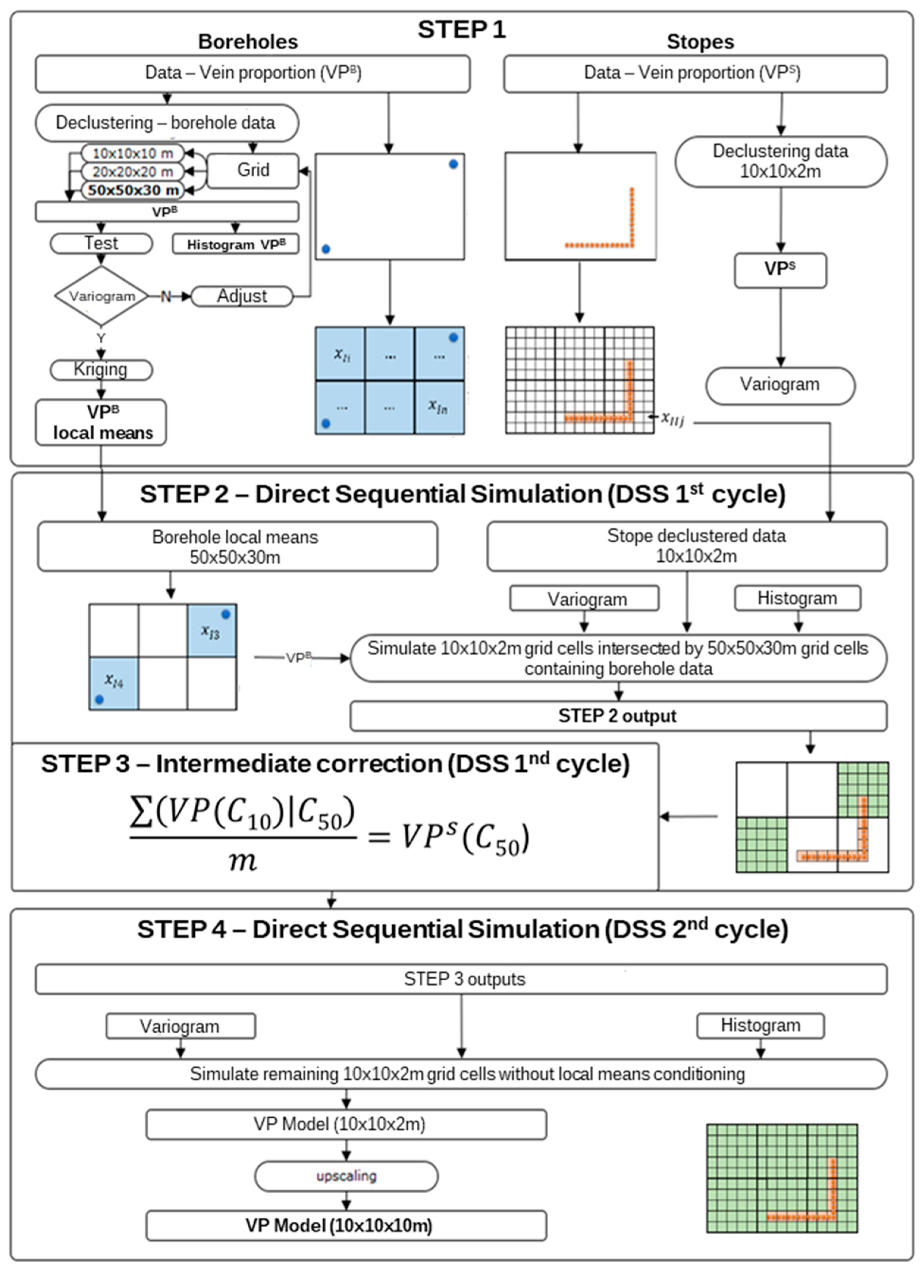
The methodology used to construct the mineral vein deposit morphology model is shown in Figure A1. This methodology consisted of four major steps, namely, grid definition and data declustering, DSS—first phase, correction of averages, and DSS—second phase.
Grid Definition and Data Declustering
In the first step, the geographic information (X, Y, and Z coordinates) and vein thickness (cm) from both data sources (stopes and boreholes) were used. Considering the final grid size (10 m × 10 m × 10 m) and the stope height (2 m), the geostatistical methods were applied using a 10 m × 10 m × 2 m grid and subsequently grouped on a 10 m × 10 m × 10 m grid.
The stope and borehole data were worked on separately in this step. The stope cumulative thicknesses were positioned on the 10 m × 10 m × 2 m grid and calculated as a vein proportion variable (vein volume by cell, VPS); where a grid cell intersected more than one stope, the arithmetic average of the values was calculated. With the VPS values having been repositioned in the centers of the grid cells, the horizontal (N–S and E–W) and vertical variograms were calculated, and the theoretical variogram models were then adjusted.
The borehole data presented a low-quality variogram with the 10 m × 10 m × 2 m grid, so the variograms for three other grid sizes (10 m × 10 m × 10 m, 20 m × 20 m × 20 m, and 50 m × 50 m × 30 m) were calculated and tested. The borehole-intersected vein values allowed the cumulative vein thickness by grid cell and vein proportion by grid cell (VPB) to be calculated. These values were georeferenced to the gravity center of the borehole segments contained in each cell, following which the VPB variable variograms were calculated. Only the 50 m × 50 m × 30 m grid presented high-quality variograms.
The grouping of the borehole information on a 50 m × 50 m × 30 m grid influenced the model as regional information, introduced as local means. The IK algorithm [16] was applied to the VPB in the 50 m × 50 m × 30 m grid to obtain the VPB histogram, and the Ordinary Kriging (OK) algorithm [16] was applied to obtain the local means.
Direct Sequential Simulation—First Phase
In the second step, the DSS algorithm [21] was applied to the 10 m × 10 m × 2 m grid cells intersected by 50 m × 50 m × 30 m cells containing borehole segments. The objective was to simulate the 10 m × 10 m × 2 m cells that are located close to boreholes, using the VPB values as soft data.
The estimation of DSS algorithm averages and variances was performed using Simple Kriging with Local Means, conditioned to the global and ungrouped VPB histogram and using the horizontal and vertical VPS variograms.
In summary, the simulation was conditioned to the stope information and structure (hard data) and to the borehole statistics (soft data).
Correction of Averages
In the previous step, DSS was used to simulate the 10 m × 10 m × 2 m grid cells (C10) conditioned to local means, but when the 50 m × 50 m × 30 m (C50) local means were compared with the 10 m × 10 m × 2 m grid homologous average values, discrepancies were identified. To correct the discrepancies between the average values, a correction is applied to the values to satisfy the following condition:
The cells containing stope data remained unchanged. Therefore, the correction of the average values was applied only to the 10 m × 10 m × 2 m cells without stope data.
Initially:
following which the average initial value is calculated:
and the correction applied as:
If VPS(C10) does not contain stope data, then the average is recalculated:
It is expected that the VP(C50)(2) value is near the value. However, if a discrepancy is still observed, then the correction of averages is applied over k cycles, until:
It should be noted that the stopes provide more detailed information and in greater quantity compared with that obtained from the boreholes. However, the measurements obtained from the stopes are spatially biased because the exploitation is conditioned to the presence of veins, reflecting a VPS average much greater than the VPB average. The proposed correction allows this effect to be attenuated near the locations of the stopes, allowing the model to more closely approximate the deposit.
Direct Sequential Simulation—Second Phase
In the fourth and final step of the morphology methodology, DSS without local means was applied to the remaining (non-estimated) cells in the 10 m × 10 m × 2 m grid, conditioned to the VPB global histogram and the VPS variograms. In this step, the simulation algorithm did not use the local means as a condition but did use the output of the third step as the basis for simulation (i.e., the corrected 10 m × 10 m × 2 m grid VPS values).
Finally, the 10 m × 10 m × 2 m grid was upscaled to a 10 m × 10 m × 10 m grid using arithmetic averages.
2.4.2. Wolframite Content Model Methodology
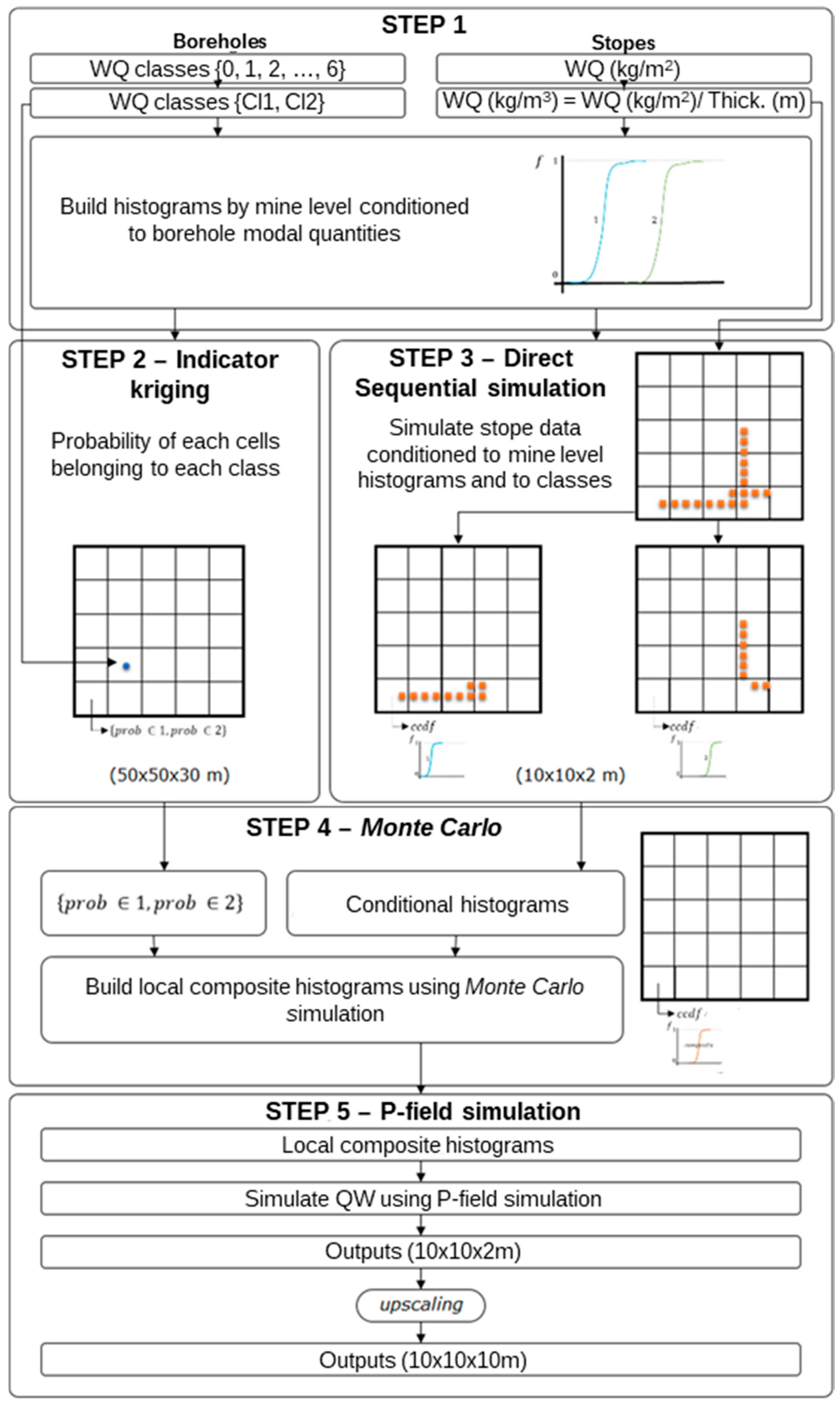
The second methodology was developed to build the wolframite content model (Figure A2) in five main steps. In this model, the stope-measured wolframite quantities were used as the principal data (hard data) and the borehole modal wolframite quantities were used as soft data. It should be noted that the modal quantity is a variable that is susceptible to observational errors and that the diameter of the boreholes does not necessarily capture the erratic occurrence of wolframite.
The stope wolframite quantity (WQ) was converted from kg/m2 to kg/m3, dividing it by the cumulative vein thickness (cm). This effectively detached the WQ from its morphological component, allowing an independent model to be built.
The Definition of Conditional Histogram Classes
The first step consisted of generating stope WQ (kg/m3) histograms for each of the borehole wolframite modal classes [0, 6]. As the stope data and borehole data are not co-localized, it was necessary, for each intersected vein (in boreholes), to identify the wolframite value of the nearest stope and assign that value to the appropriate class. The search was limited to 50 m in the horizontal direction and 15 m in the vertical direction. In each case where more than one stope was identified within the search radius, the average wolframite value of the identified stopes was assigned to a class.
After every borehole wolframite modal class had been assigned a value from the nearest stope(s), it was possible to build the histograms and examine the discrimination of the classes. This procedure allowed the number of classes to be reduced by associating them by behavioral similarity. From this step, two or three grouped classes resulted.
Indicator Kriging
In the second step, the IK algorithm [16] was applied to the grouped borehole WQ classes to estimate the probability of each cell belonging to each new class. The estimation was made on a 50 m × 50 m × 30 m grid, but the results were replicated to a 10 m × 10 m × 2 m grid.
Building the Conditional Local Distribution Laws of Wolframite Quantity
In the third step, the local distribution laws of WQ were determined conditioned to each grouped class from boreholes by simulating n equiprobable scenarios for each grouped class and mine level, using the DSS algorithm [21].
For each stope, the nearest borehole-intersected vein was selected and was associated with the respective modal class defined in the first step of the methodology.
To estimate the regional histograms for each mine exploitation level, the IK algorithm was applied to the WQ in the whole model, and the results were recorded by level (L0, L1, L2, and L3).
Conditioning the simulation to regional histograms increases the coherence of the simulated results because a large fraction of the simulated region is far from the boreholes and because there is a segregation of regional WQ with depth.
After n scenarios were simulated by cell and class, each set of n values for each cell constituted the intended conditional distribution law.
Building the Composite Local Distribution Laws of Wolframite Quantity
This step combined the probability of each cell belonging to each grouped class (step 2) with the conditional local distribution laws of WQ (step 3). The composite local distribution laws of WQ were obtained by mixing the individual histograms weighted by the estimated probabilities, using Monte Carlo simulation.
The composite histograms obtained in each cell of the model constitute an estimate of the law of distribution that considers the stope-derived wolframite quantities and the borehole-derived modal quantities. At the exact location of a stope, the composite law has zero variance and an average equal to the stope wolframite quantity value. At the exact location of a borehole-intersected vein, the estimated probability (step 2) is 1 for the borehole-derived class and 0 for the other classes, and therefore the composite histogram coincides with the distribution law of the class with 100% probability. In all other cases, the variance is proportional to the distance from the nearest stope.
Simulating Maps of Wolframite Content
In the fifth and final step, once the WQ distribution law for each cell was known, WQ maps were simulated using Probability Field Simulation (PFS) [22]. Finally, the results, in a 10 m × 10 m × 2 m grid, were vertically upscaled to a 10 m × 10 m × 10 m grid using arithmetic averaging.
3. Results
The methodologies presented in Section 2 (for morphology and wolframite content) were applied to the Mine Database provided by the relevant mining company. For reasons of confidentiality, all wolframite contents are rescaled to the interval [0, 1], and XY coordinates are defined locally. To easily compare the outputs, all the section images correspond to Px81 (YoZ projection, X = 805 m) and all the section images correspond to Pz75 (XoY projection, Z = 620) (Figure 2).
3.1. Data and Grids
The information provided includes data from two sources: stopes and boreholes. The database contains information from 2759 boreholes drilled between 1971 and 2014, representing 113,012.53 m of sampled core and 20,992 intersected veins. The borehole database has the following different fields: borehole code/ID; origin coordinates (X, Y, Z); borehole length; average azimuth; and average dip. For each intersected vein, the initial and final intersection depths, the difference in depth in cm (i.e., vein apparent thickness), and the modal quantity of wolframite in seven modal classes (0 representing absence and 6 representing abundance) are registered in the database. The stope database has 59,047 entries, each corresponding to a sampling panel. The stope database contains fields reporting the gallery base coordinates (X, Y, Z) panel height (usually 2.2 m), vein thickness, and the quantity of wolframite (kg/m2).
3.1.1. Stopes
To build the morphology model, a vein proportion variable (VPS) is defined taking into account the average height of the stope accesses (2.2 m), according to the following equation:
All the VPS calculations assume that the veins are near horizontal and that the vertical sampling panels intersect the veins at 90°.
To separate WQ from its morphological component and thereby create an independent model, the stope WQ is converted to kg/m3, dividing it by the cumulative thickness:
The modelling steps using stope data are performed using a 10 m × 10 m × 2 m grid. The stope grid (10 m × 10 m × 2 m) settings are summarized in Table 1. The grid contains 4,819,500 cells.
3.1.2. Boreholes
The borehole data are modelled on a 50 m × 50 m × 30 m grid owing to the study of the VPB variable variography, as presented in Section 3.1.1. The borehole grid (50 m × 50 m × 30 m) settings are summarized in Table 2. The grid contains 12,852 cells. The amplitude between mine levels L0 and L3 is 270 m; a cell height of 30 m is used after variogram range calculations and sensitivity analysis.
In the borehole data, the thickness of intersected veins is also converted to VPB. In this case, the cumulative vein thickness is divided by the cumulative borehole segment lengths inside each 50 m × 50 m × 30 m cell:
3.1.3. Final Grid
Finally, the results of each methodology are upscaled to a 10 m × 10 m × 10 m grid. The grid geometry is presented in Table 3 and contains 963,900 cells.
3.2. Univariate Data Analysis
This section presents a univariate statistical analysis of the different variables from stopes and boreholes, namely, vein thickness, VP, and WQ.
3.2.1. Stopes
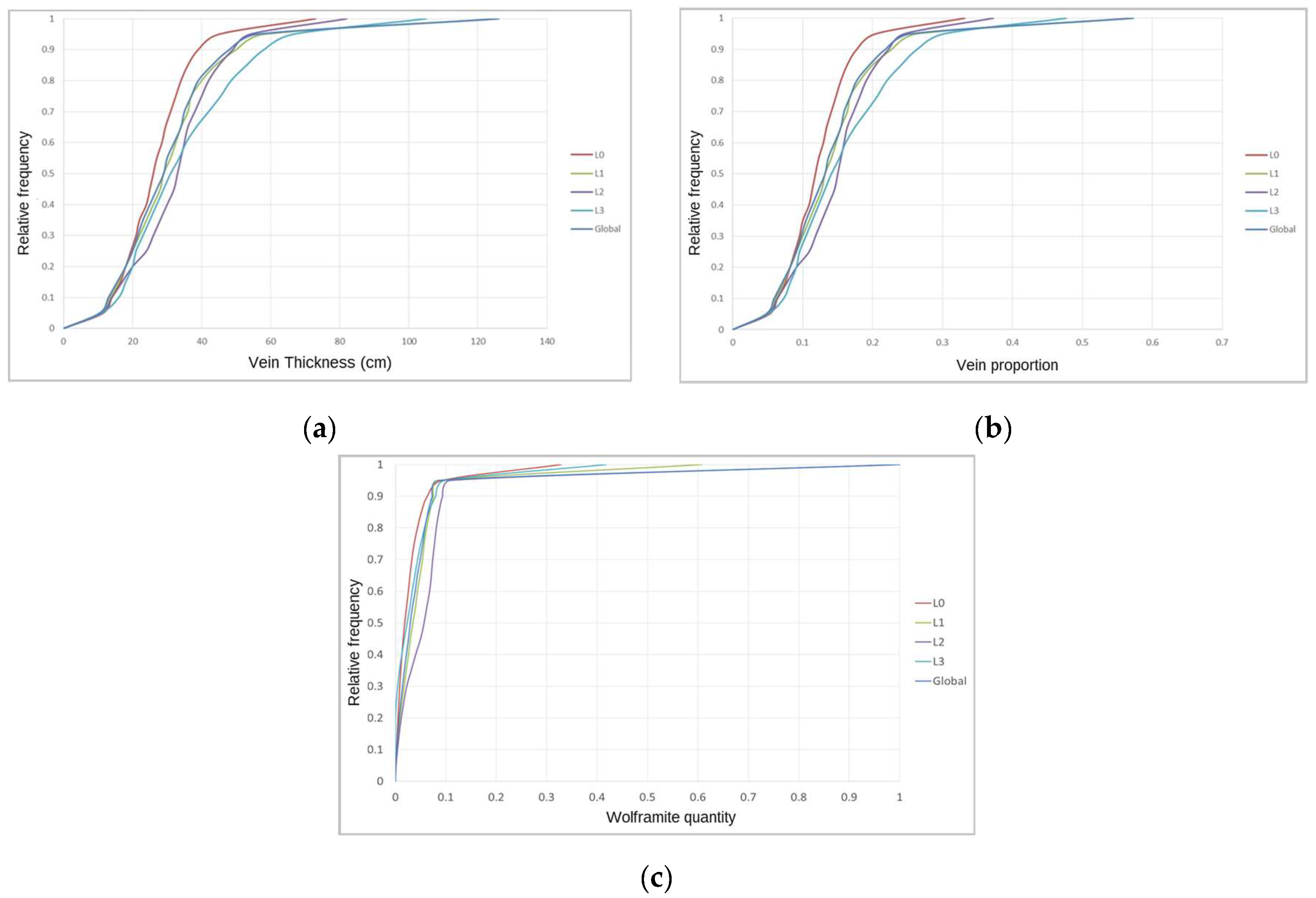
Table A1 and Table A2 report the results of the univariate statistical analysis applied to the stope vein thickness and VP variables. The global average vein thickness is 31.5 cm. When the analysis is applied by level, it reveals that the lowest values are found in L0 and that the values increase with increasing depth. Levels L3 and L1 present the highest dispersion in vein thickness values, followed by L2 and L0. The thickness range is from 0 (no vein) to 126 cm, and the thickest veins occur in L1 and L3. All levels present positively skewed histograms, revealing the predominance of low values. The cumulative histograms of vein thickness (Figure A3a) and VP (Figure A3b) show these described behaviors. As the VP is obtained by dividing the vein thickness by a constant value, vein proportion is proportional to vein thickness; the VPS average value is 0.143 (14.3%).
Using the same statistical functions, a statistical analysis was applied to the stope WQ variable (in kg/m3), the results for which are given in Table A3. The WQ global average is 0.046 kg/m3, although WQ varies with depth. The richest levels are L2 and L1, with the poorest levels being L0 and L3, in that order. All the levels show high dispersion, with deviations from the average ranging between 70% and 120%. The highest values of WQ occur in L2 and L1. Regarding the morphology variables, the skewness coefficient of the distribution of WQ presents high values, indicating that there are more low values of WQ than high values. The cumulative histograms for WQ are shown in Figure A3c.
3.2.2. Boreholes
Table A4 presents the univariate statistical results for borehole-intersected vein thickness, and Figure A4a shows the variable cumulative histograms. As with the stope results, the borehole results show an increase in vein thickness with increasing depth. The average value is 11.7 cm (cf. stope average value 31.5 cm). This difference between the two average values reflects the aforementioned sampling bias in stopes and also means that the skewness and dispersion measurements for the borehole-derived values are higher than for the stope-derived values.
A global estimation of stope vein proportion (VPS) was calculated by dividing the sum of vein thicknesses (246,031.6 cm) by the sum of borehole lengths (11,301,253 cm):
The global VP in boreholes is 0.022 (2.2%), approximately seven times lower than in stopes. This differential can be explained in terms of the sampling bias of veins in the stopes compared with the boreholes. The statistical analysis was also applied to each level (results in Table A5 and cumulative histograms in Figure A4b) by converting the borehole data to a regular pattern (50 m × 50 m × 30 m grid). The dispersion coefficient of VP presents lower values compared with vein thickness, and although the skewness is positive, it is lower than that of vein thickness, mainly because the conversion of the variables involves the calculation of averages.
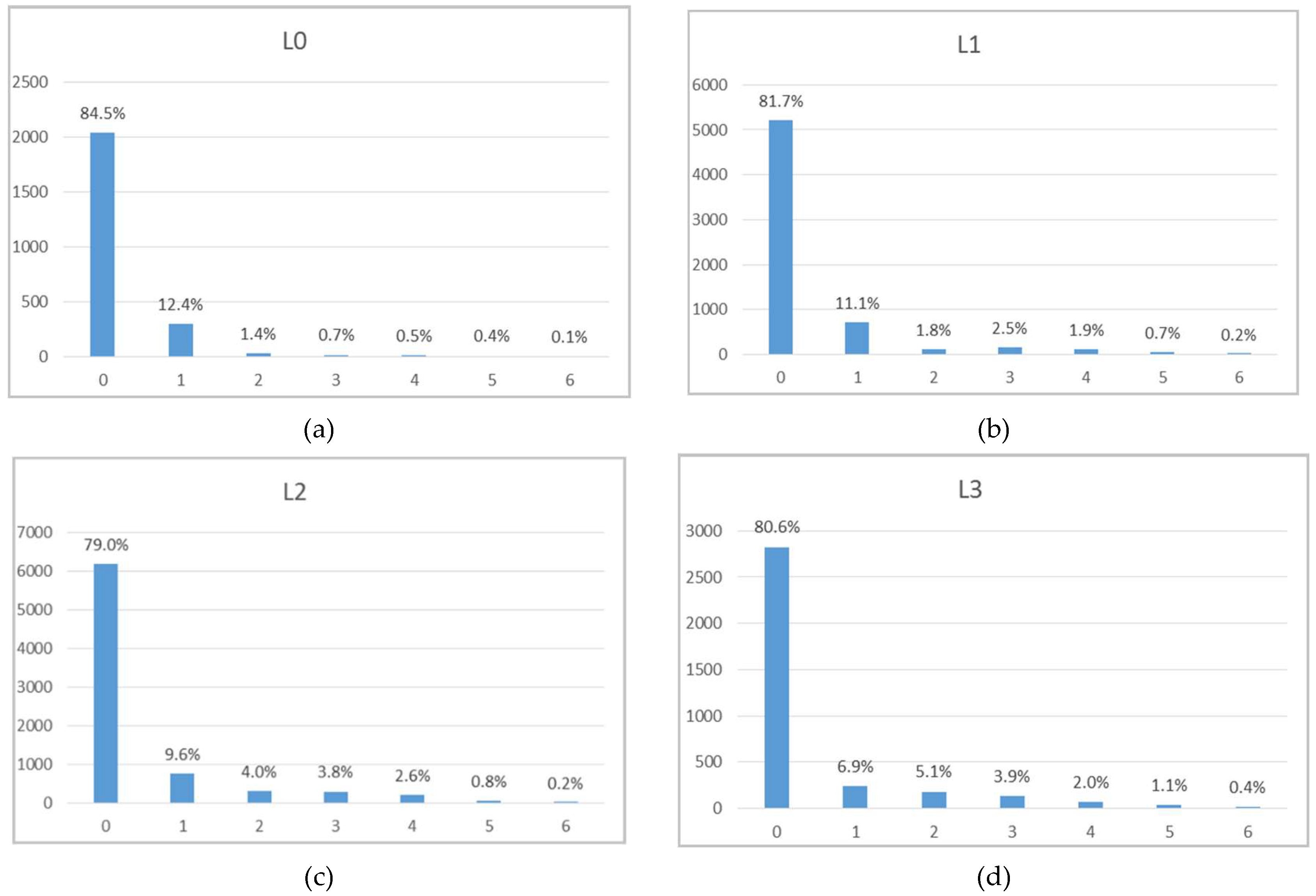
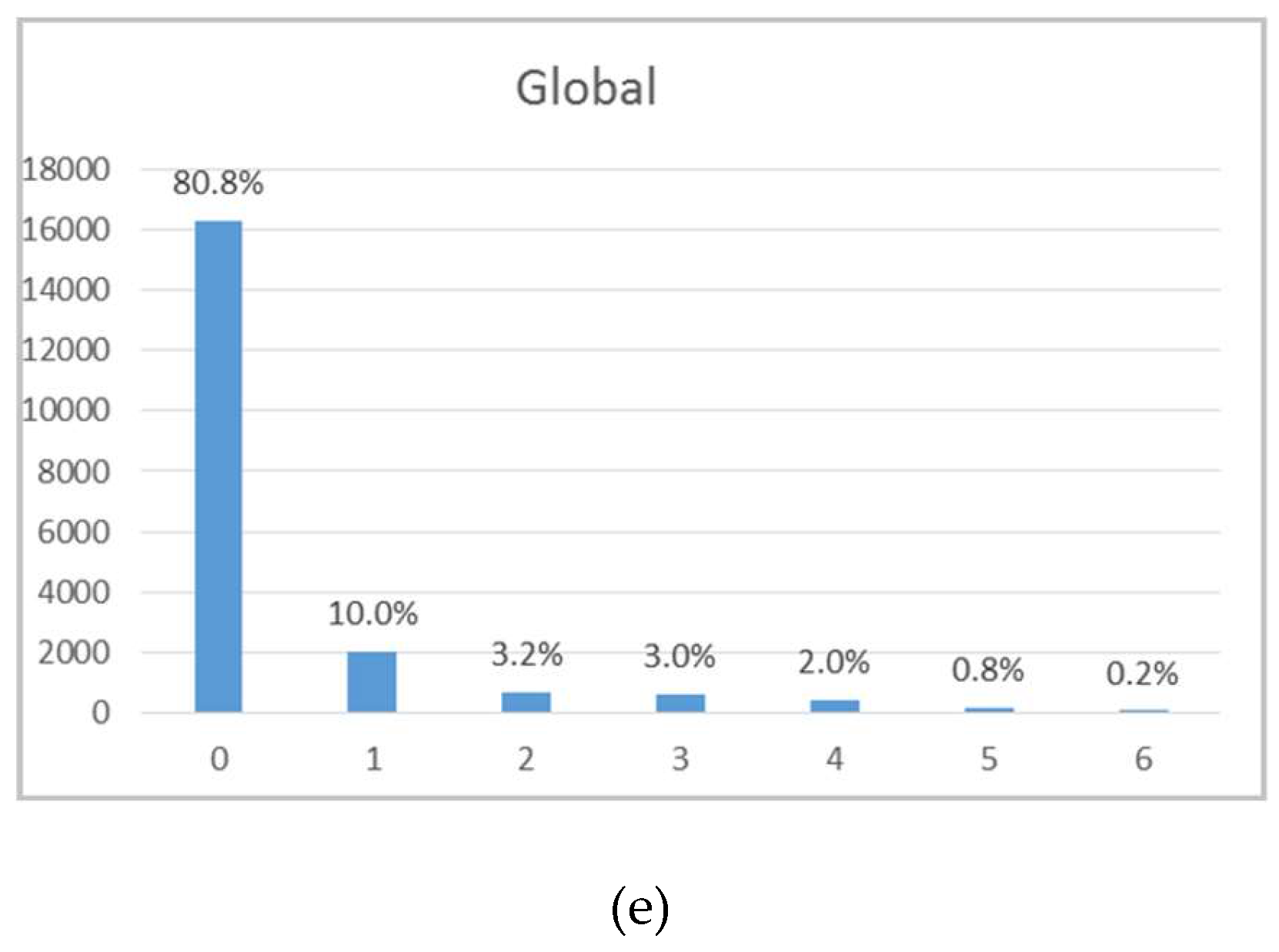
Finally, the statistical analysis was applied to the borehole wolframite modal quantity. This variable has seven classes, with 0 representing wolframite absence and 6 representing abundance. Table A6 reports the statistical results and Figure A5 shows the frequency histograms by level (A5a–d) and globally (A5e). Eighty percent of the intersected veins belong to class 0, followed by class 1 (10%).
3.3. Morphology Modelling
3.3.1. Grid Definition and VPS Variography
In the first step of the morphology methodology, different grid sizes were tested to obtain good variogram adjustments. The definition of the grid size should meet certain conditions, such as the existence of an adjustable variogram and the multiplicity between the grid vertical dimension (30 m) and the mine vertical amplitude (270 m). As noted in Section 2.4., the 10 m × 10 m × 10 m and 20 m × 20 m × 20 m grids do not present adjustable variograms (Figure A6). The regularization of the borehole data to a regular grid helps to overcome proximal incongruencies such as high values near low values.
A 50 m × 50 m × 30 m grid was tested, for which the horizontal dimension of 50 m allows more boreholes to be incorporated in one cell (compared with the smaller grids) and the mine vertical amplitude is a multiple of the 30 m vertical dimension. In the 50 m × 50 m × 30 m grid, the variogram adjustments resulted in high correlation amplitudes, 350 m in the horizontal direction (Figure A7a) and 170 m in the vertical direction (Figure A7b). The variograms and adjustment settings are presented in Table A7.
3.3.2. VPB Kriging Using a 50 m × 50 m × 30 m Grid
The IK algorithm was applied to generate the VPB global disaggregated histogram to condition the simulations. A total of 20 VPB classes were simulated with the same amplitude, using the variograms obtained in the previous step.
The disaggregated histogram average is 0.014, much lower than the aggregated data average (0.022). This difference can be explained by the ungrouping process, which includes sub-sampled parts of the deposit in the calculation of averages.
Also in this step, an Ordinary Kriging (OK) algorithm was applied to the three-dimensional space, in the 50 m × 50 m × 30 m grid, with VPB variograms to estimate a VPB map (Figure 3), used as local means in the ensuing steps.
3.3.3. VPS Declustering and Variography Using a 10 m × 10 m × 2 m Grid
The first step of the flowchart (Figure A1) ends with the declustering of VPS (Figure 4), by arithmetic averaging, on a 10 m × 10 m × 2 m grid, followed by the calculation and adjustment of variograms (Table A8). The declustered data show high spatial continuity, presenting variogram amplitudes in the order of 600 m (isotropic) in the horizontal direction (Figure A8a,b) and 40 m in the vertical direction (Figure A8c).
3.3.4. Direct Sequential Simulation First Phase Plus Correction of Averages
The second step of the methodology starts by simulating vein proportion using the DSS algorithm, on a 10 m × 10 m × 2 m grid, conditioned to the VPS declustered histogram and to the VPB local means. The DSS is conducted using the stope declustered data as hard data. One thousand scenarios are generated because there are poorly conditioned zones in the model.
Figure 5 represents one of the 1000 simulated scenarios. As explained in Section 2.4, the DSS first-phase outputs are 10 m × 10 m × 2 m cells, corresponding to 50 m × 50 m × 30 m cells containing borehole segments, homologous 10 m × 10 m × 2 m cells, and 10 m × 10 m × 2 m cells with stope data.
Although the DSS algorithm uses Simple Kriging with Local Means to estimate the averages and variances, the 10 m × 10 m × 2 m results when grouped and compared with the homologous 50 m × 50 m × 30 m cells do not have the same average, so it is necessary to apply a correction of averages for the simulated values (methodology step 3). In this step, there is a global tendency to lower the simulated values (Figure 6), maintaining those intersected by hard data (stope data).
3.3.5. Direct Sequential Simulation Second Phase and Final Model Interpretations
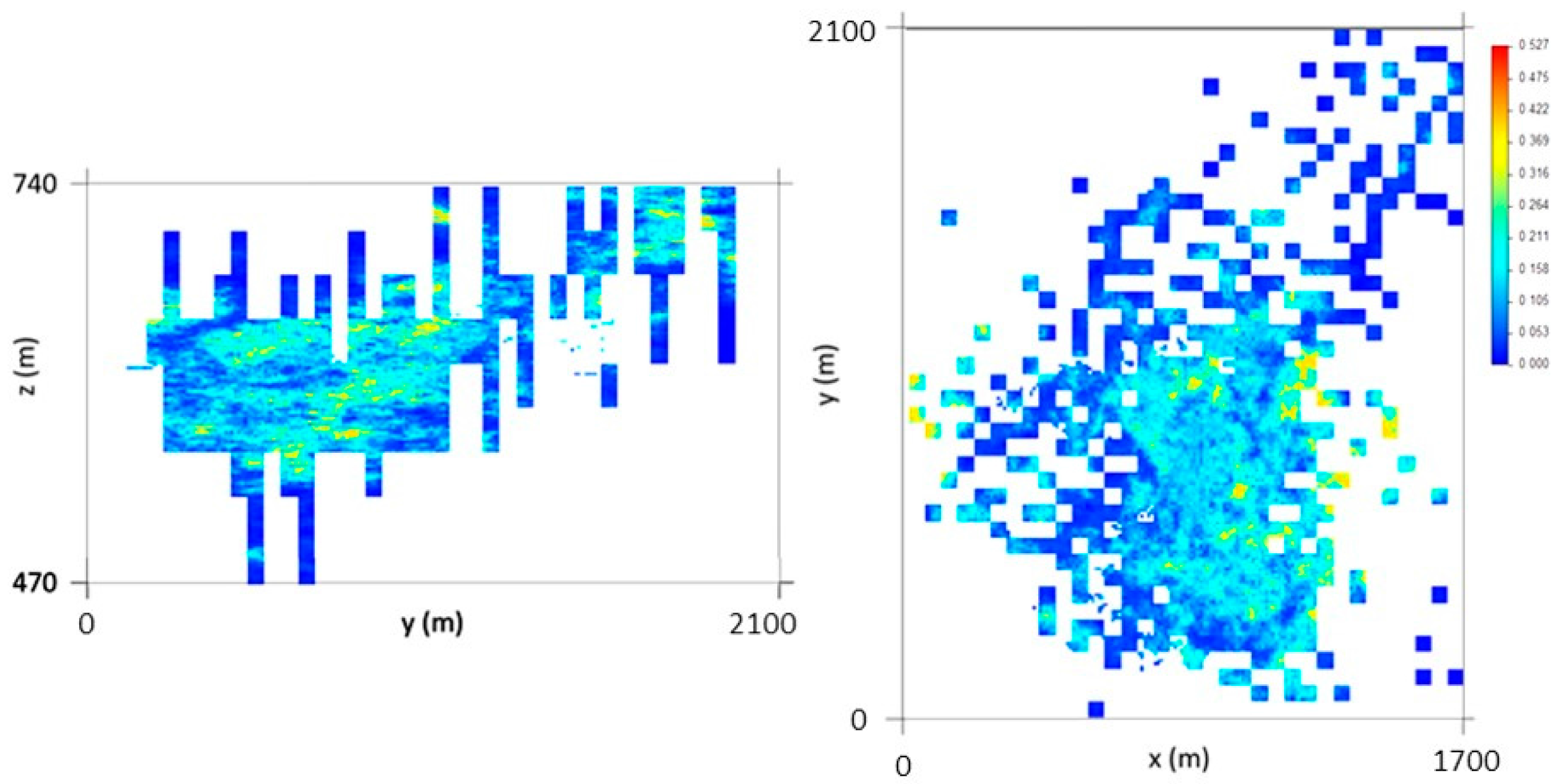
The last step is to apply DSS to the remaining non-estimated cells without conditioning to local means but conditioned to the previous outputs (10 m × 10 m × 2 m simulated cells), to the VPB histogram, and to the VPS variograms (both horizontal and vertical). Figure 7 presents the final VP map.
At the end of this step, a vertical upscaling to the 10 m × 10 m × 10 m grid is made, and the maps of the VP average and coefficient of variation (CV) are calculated using 1000 simulated scenarios. By analyzing the average map (Figure 8), it can be seen that the thickest veins occur in the central part of the deposit, corresponding to L1 and L2.
The coefficient of variation (CV) image (Figure 8) shows that zones of higher uncertainty are located in the peripheral parts of the model, a result of the lower amounts of information in those parts, and that there is zero uncertainty in the locations of the stopes, respecting the VPS (hard data). Some high CV values in the central part of the model can be explained by high data density or by high difference amplitudes between cells located in close proximity to each other.
After the final images of VP had been obtained using DSS, the variograms of the first scenario of each step of the methodology were calculated and adjusted with the same parameters of the initial variograms (by 600 m horizontally and 40 m vertically) to verify how well the images reproduced the variograms. The adjustment of the variograms shows that there is some discrepancy between the steps. The DSS (step 1—Figure A9a,b) respects the initial data structure. After the correction of averages (step 3—Figure A9c,d), the spatial continuity decreases significantly, mainly because the correction of averages forces an alteration in the values, increasing the discrepancy between the neighboring cells of the model and consequently distorting the variogram. In step 4 (Figure A9e,f), another application of DSS reimposes the variogram and approximates the simulation output spatial structure to the original.
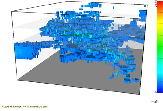
Figure 9a,b show the 3D representation of the final VP model and the CV model, respectively.
3.4. Wolframite Content Modelling
3.4.1. Correlation Analysis between Stope Wolframite Quantities and Borehole Wolframite Modal Quantities
The first step of the methodology consists of analyzing the correlation between stope wolframite quantities and borehole wolframite modal quantities, which allows the seven classes of wolframite modal content to be grouped into only two, representing high and low wolframite quantities, as follows.
Conditional cumulative global histograms for each class were built, and the results showed that the histogram classes that best discriminate WQ are 0, 1, and 2, with the other four classes presenting poor discrimination. To improve the result, the same process was replicated but additionally conditioning the histograms by level (e.g., L0 in Figure 10a). This solution proved to be the most viable when the classes were grouped into two broader classes, joining classes {0–1–2} and classes {3–4–5–6}, by level (e.g., L0 in Figure 10b).
The levels with better discrimination of WQ are L0 and L3, with L1 and L2 showing essentially no discrimination. It would be expected that the borehole-derived wolframite classes would have a better correlation with the stope data; however, this was not observed, possibly because there is too much randomness in wolframite occurrence in the veins, being hardly intersected by borehole cores, and because the two sources of information are rarely co-located. However, it seems to be advantageous to use the proposed methodology for levels L0 and L3, given that in L1 and L2, owing to poor discrimination, the grouping into two broader classes does not influence the obtained model. Hereafter, the grouped classes are designated CL1 {0, 1, 2} and CL2 {3, 4, 5, 6}.
3.4.2. CL1 and CL2 Indicator Kriging Using a 50 m × 50 m × 30 m Grid
In the second step, IK is applied to estimate the probability of each 50 m × 50 m × 30 m cell belonging to CL1 or to its complementary class, CL2. As there are only two classes, it is sufficient to estimate Prob {CL1}, and then Prob {CL2} = 1 − Prob {CL1}.
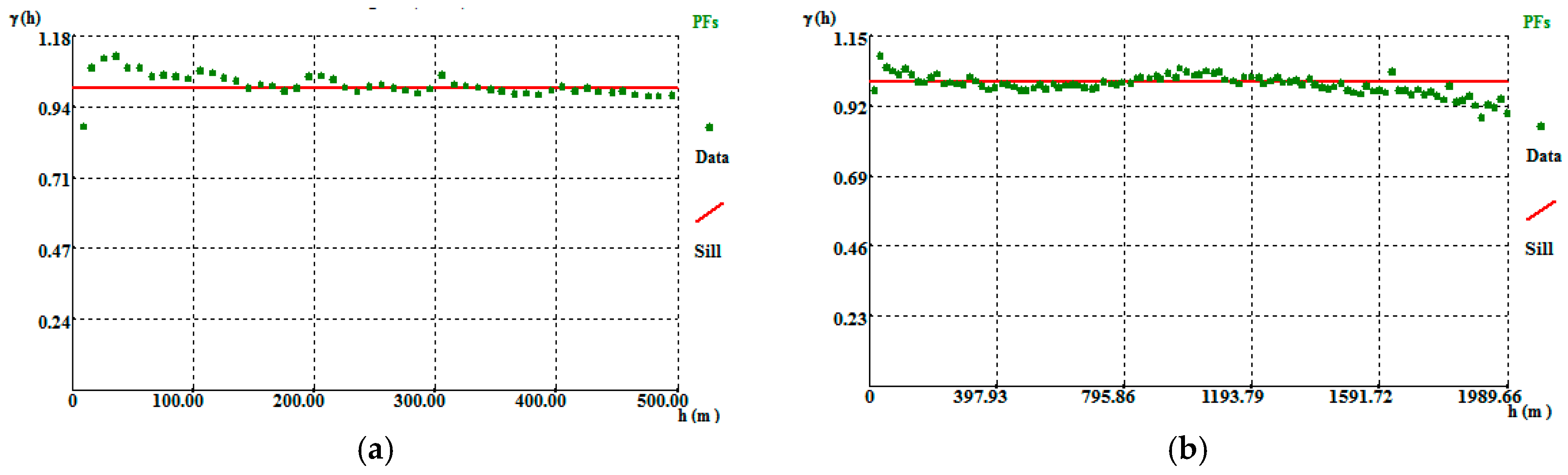
Before applying the IK algorithm, variograms of the indicator variable were calculated and adjusted, the parameters and results of which are reported in Table A9. The adjustments were made using an exponential structure and model, revealing amplitudes of 70 m in the horizontal direction (Figure A10a) and 50 m in the vertical direction (Figure A10b).
The IK outputs (Figure 11) reproduce the higher probability of a cell of the model belonging to the classes grouped in CL1, with an average value (93.8%), close to the initial data average (94%). It should also be noted that in the northern part of the deposit, the estimated CL1 probabilities are close to 100%, representing the low-quantity wolframite class.
3.4.3. DSS of Wolframite Quantity Conditioned to CL1 and CL2 Histograms Using the 10 m × 10 m × 2 m Grid
In the third step, DSS was used to generate WQ scenarios conditioned to CL1 and to CL2, with conditional histograms being produced by each level (Step 1).
So that the stope data (hard data) could be used, the data of each stope was classified as CL1 or CL2 according to the WQ class of the nearest borehole (search radius 50 m in the horizontal direction and 15 in the vertical direction), splitting the stope data into two different data sets. To include all stope data in the DSS, in cases where the search region did not include borehole data, the stope entry was added to both data sets.
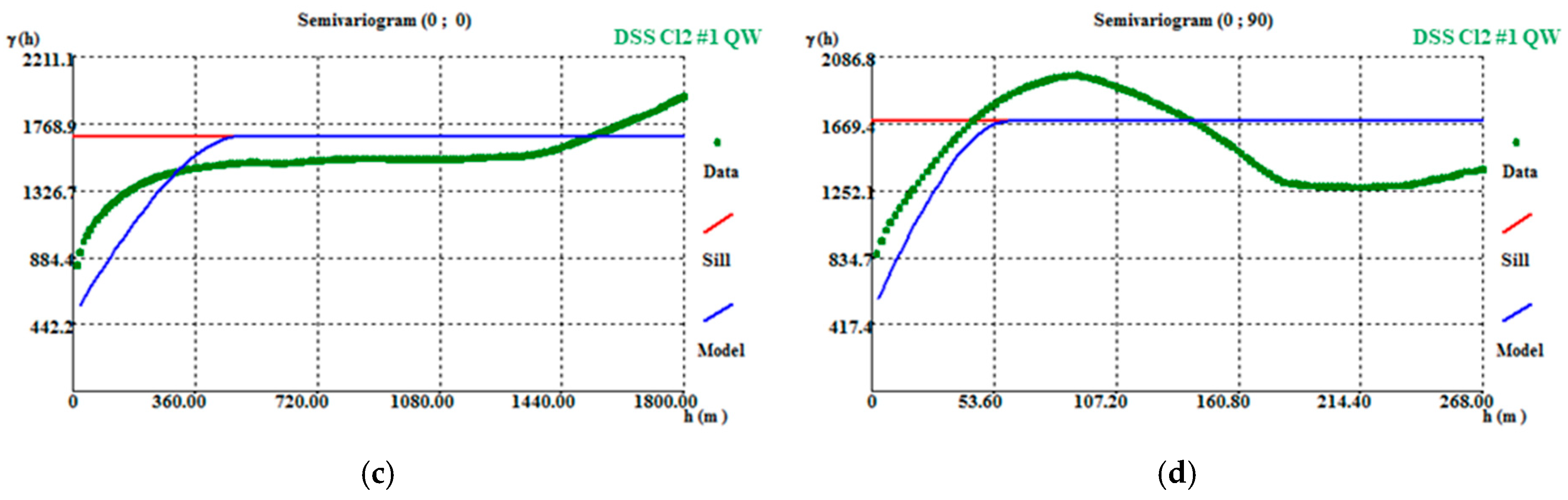
The stope WQ (kg/m3) variograms were calculated for the whole data set (i.e., before splitting the data). The variogram calculation parameters are reported in Table A10. Variogram adjustment was made with a 30% nugget effect, 500 m of horizontal amplitude (Figure A11a), and 60 m of vertical amplitude (Figure A11b).
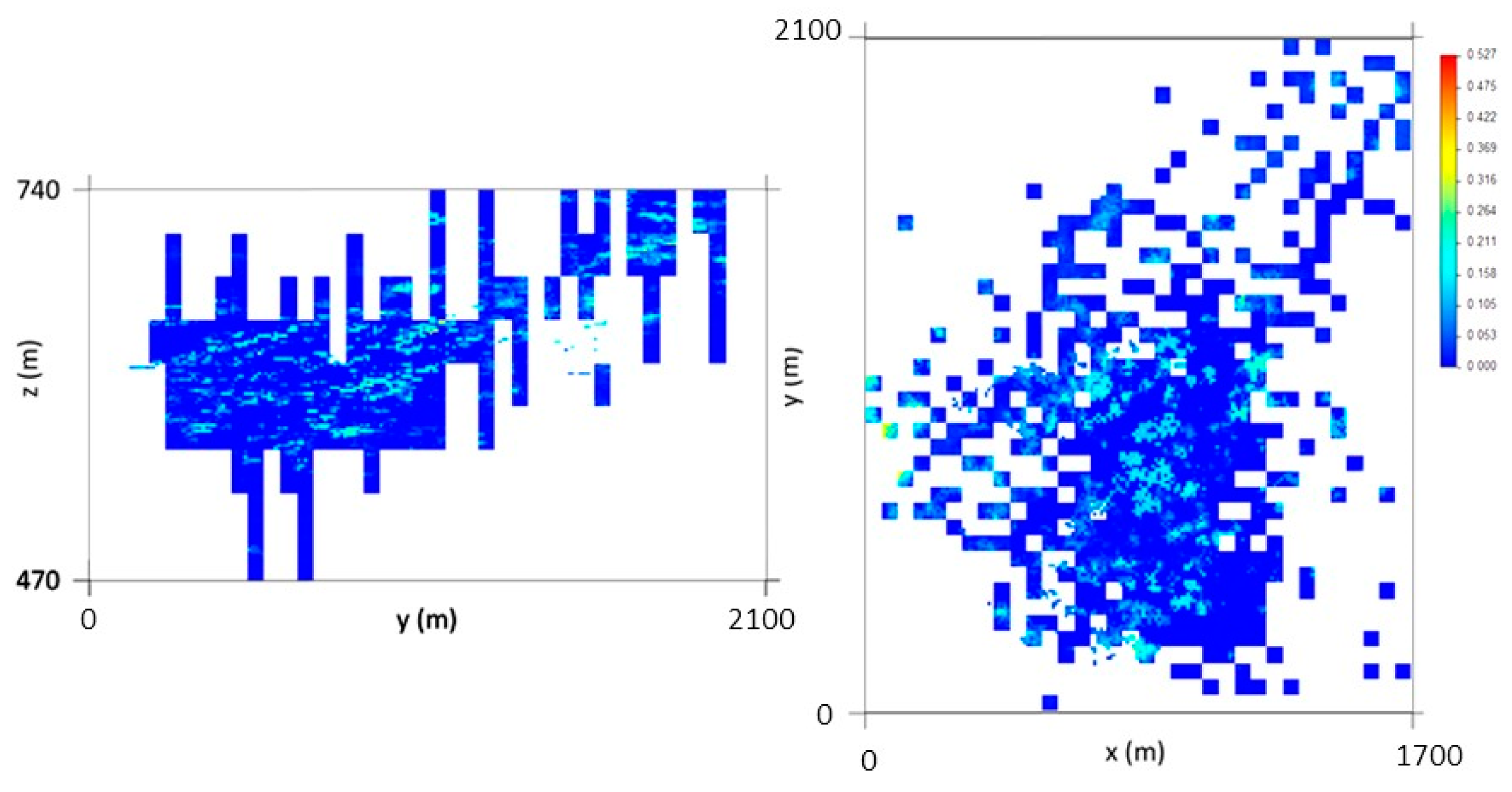
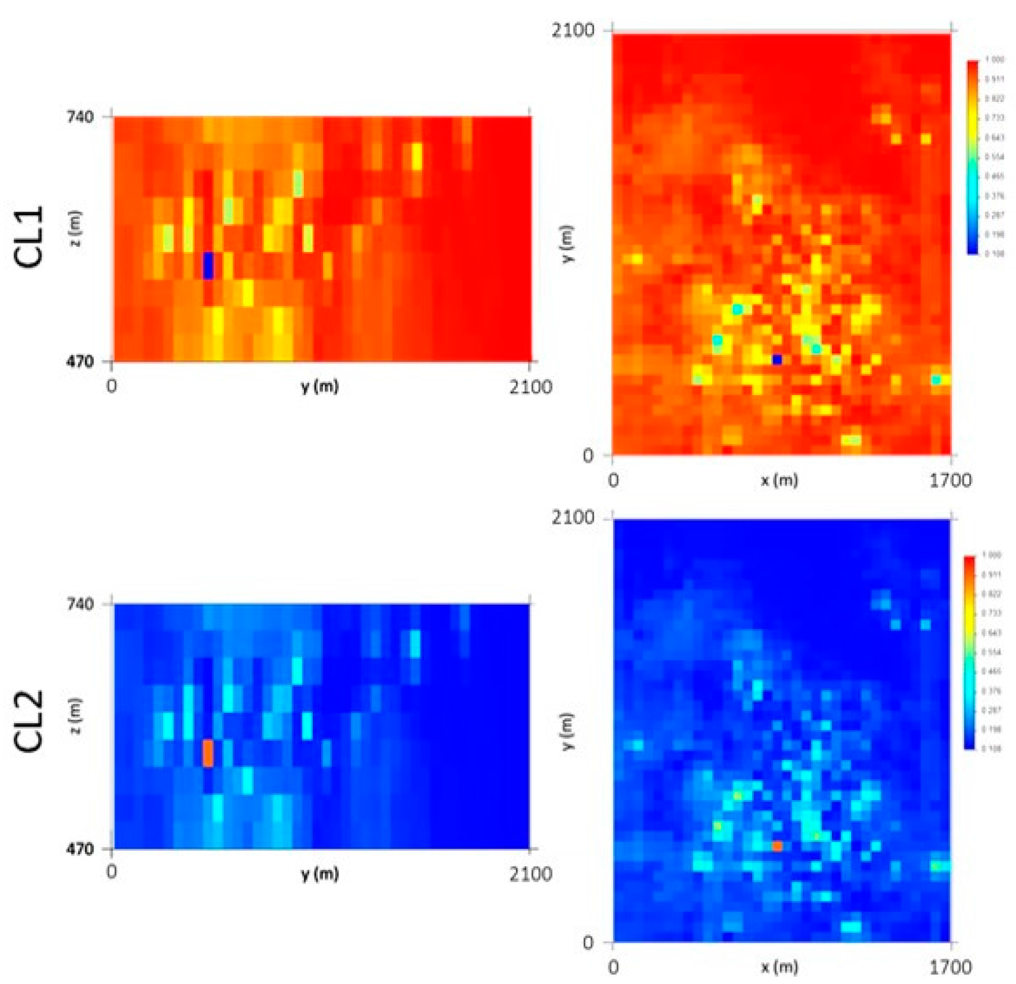
Two hundred WQ scenarios were simulated for each class (CL1 and CL2) to build the conditional cumulative histograms in each grid cell (local distribution laws). Figure 12 presents the first of 200 simulated scenarios for CL1 and CL2, in which it is possible to observe the 30% nugget effect (high values among the low values) and the influence of the level-related histogram condition (high values in the L2 layers).
To validate the results, the first simulated scenario variograms were calculated and validated, for both classes, using the same parameters (500 m in the horizontal direction, 60 m in the vertical direction, and 30% nugget effect) as used for the variograms for the initial data. The variograms of the simulated maps for both classes show an offset when compared with the variograms of the initial data (Figure A12a,b), which arises because the original variography study uses the whole data set and the simulations are conditioned to the split stope data.
3.4.4. The Generation of Wolframite Quantity Distribution Laws for Each Cell
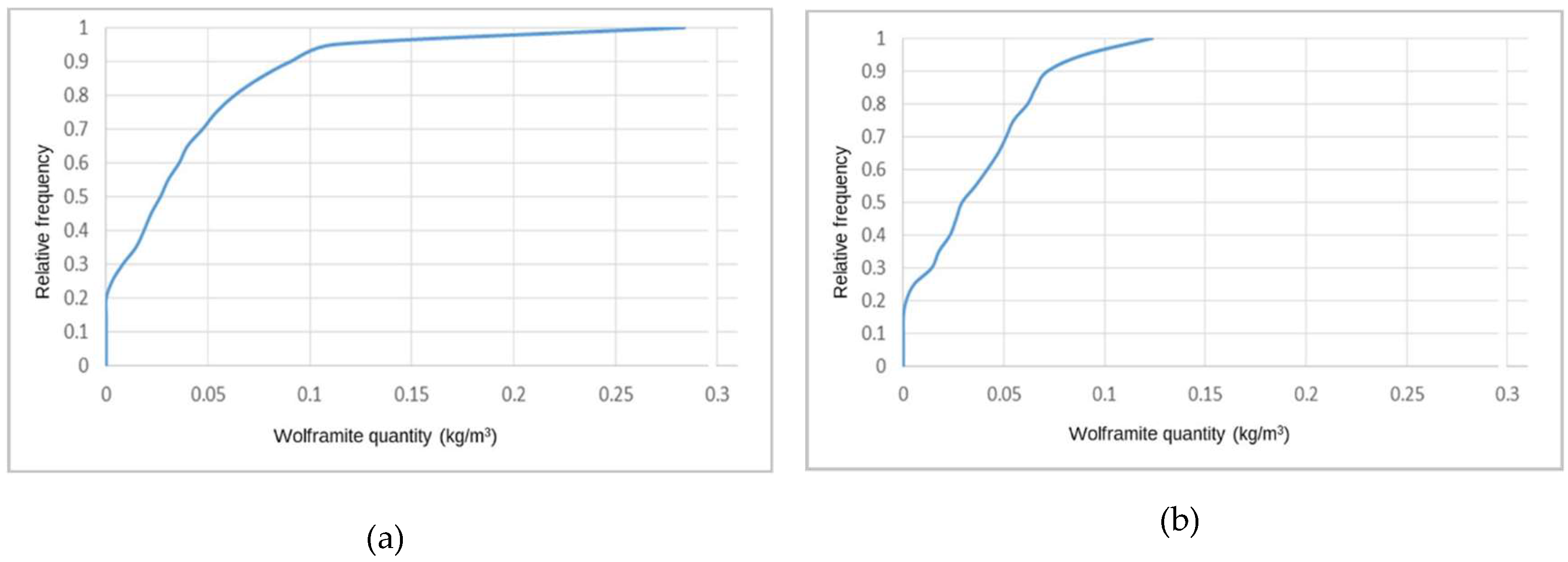
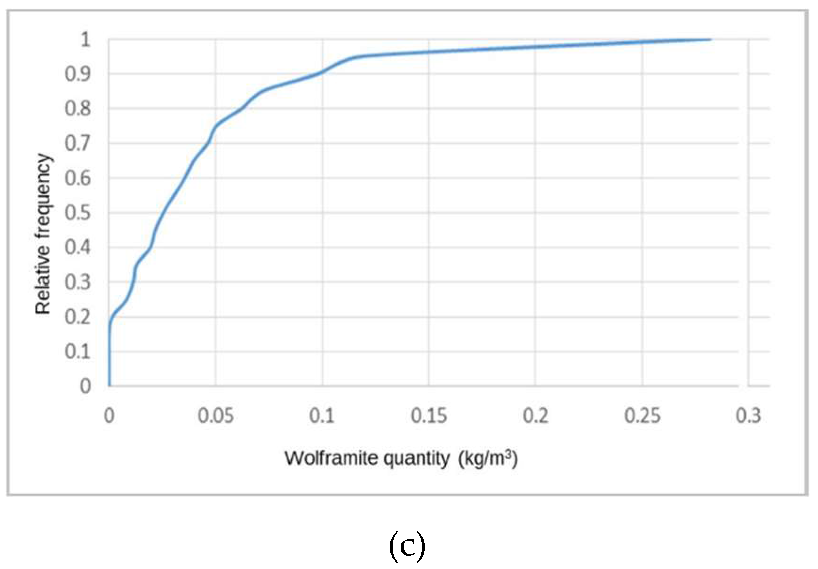
In step 4, Monte Carlo simulation was used to build the local distribution laws for each grid cell by crossing the IK estimated probabilities (step 2) with the local conditional cumulative histograms for classes CL1 and CL2 (Step 3). In the example given in Figure 13, corresponding to the first cell of the model, the probabilities are Prob {CL1} = 0.9159 and Prob {CL2} = 1 − Prob {CL1} = 0.0841. Therefore, using 100 values to build the composite cumulative histogram for each model cell, 92 values from the CL1 cumulative histogram (Figure 13a) and eight values from the CL2 cumulative histogram (Figure 13b) were extracted using the Monte Carlo procedure.
Figure 13c corresponds to the composite cumulative histogram of the first model cell. As the CL1 probability is high (92%), the resultant curve is very strongly influenced by the structure of the CL1 histogram.
3.4.5. Probability Field Simulation Using the 10 m × 10 m × 2 m Grid and Final Model Interpretations Using the 10 m × 10 m × 10 m Grid
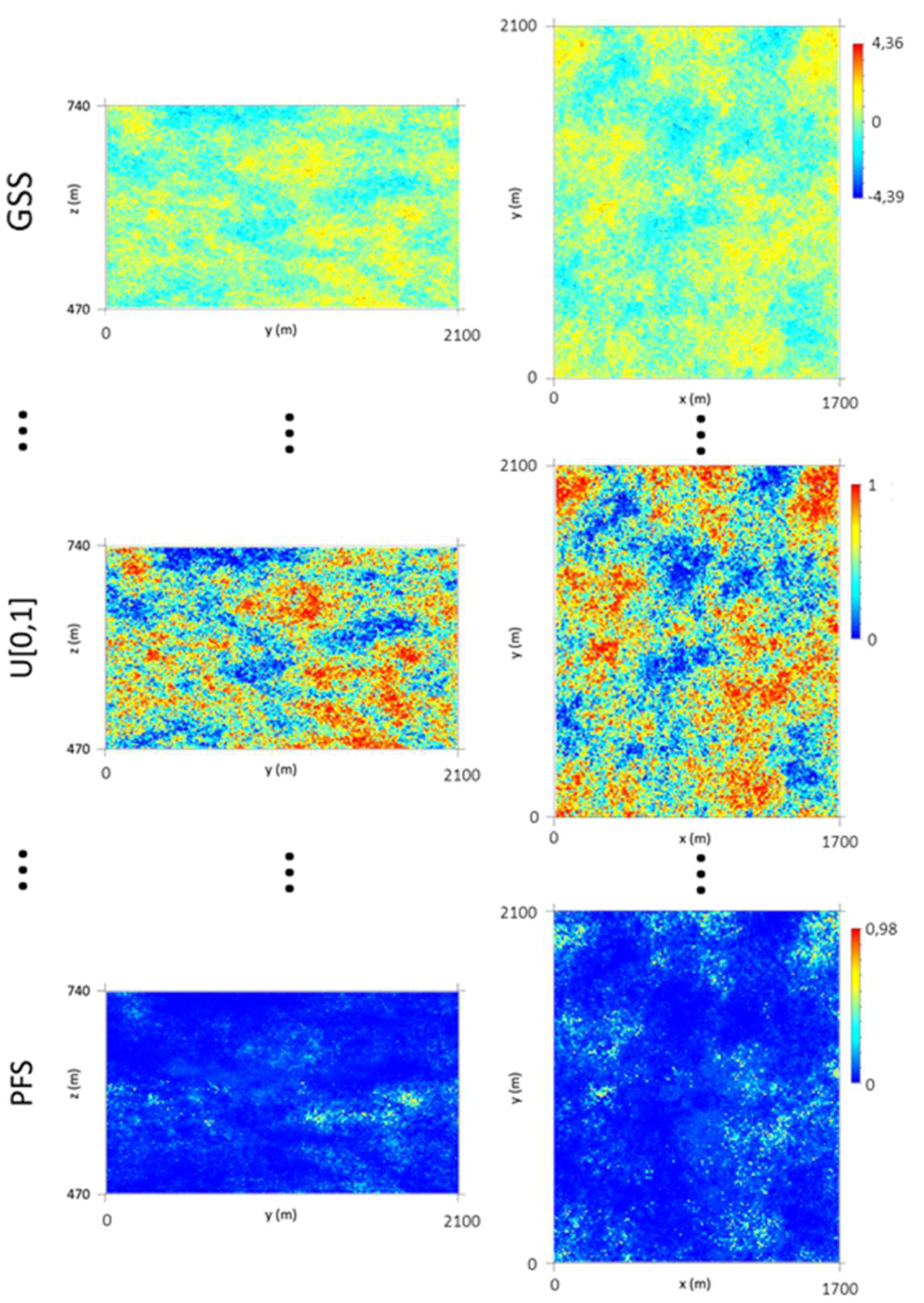
In the final step, the WQ maps were simulated using PFS. As the variograms exhibit a marked nugget effect, 1000 simulated scenarios were generated to properly quantify the model uncertainty.
As a basis for the PFS application (Figure 14), 1000 probability maps with a uniform distribution law (U [0, 1]) were generated by transforming the outputs of 1000 simulated scenarios obtained using Gaussian Sequential Simulation (GSS). The GSS algorithm was applied based on the stope variograms. Finally, the PFS algorithm was run based on the U [0, 1] scenarios, the local composite cumulative histograms, and the stope WQ variograms.
A comparison of the stope WQ statistics for the initial data with the first scenario of the PFS shows that the extreme (minimum and maximum) and average values are the same (Table A11). The median value of the first scenario of the PFS is significantly lower, and the variance and skewness are higher, because the estimation of the probability of belonging to each class has a degradational effect on the data. This phenomenon is most clearly expressed in the peripheral zones of the model, where the stope wolframite quantities are lower, generating more accentuated right-skewed distribution laws.
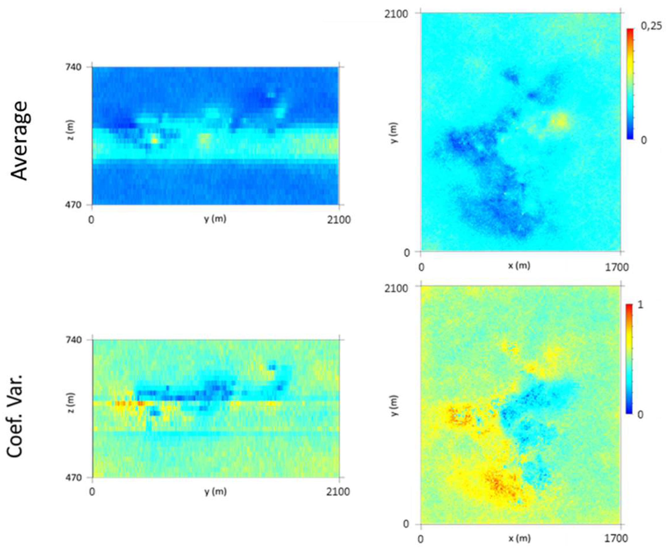
Finally, the model (10 m × 10 m × 2 m grid) was vertically upscaled to a 10 m × 10 m × 10 m grid, and maps of the average and CV were calculated (Figure 15). By analyzing the average map, it can be seen that the richest level is L2, followed by L1. The uncertainty of the model is higher in the peripheral parts of the model, and lower in the stope-sampled zones. However, a zone of high dispersion is evident in the L2 sampled region, mainly in the southwestern part of the deposit, where the original data are heterogeneous (wide discrepancies between close values), which forces the simulation to generate different values between different scenarios.
3.5. Estimation of the Deposit’s Mineral Potential
After implementing the independent methodologies for estimating VP and WQ and validating the results, the models were crossed using a 10 m × 10 m × 2 m grid, for each of the 1000 scenarios, using Equation (11).
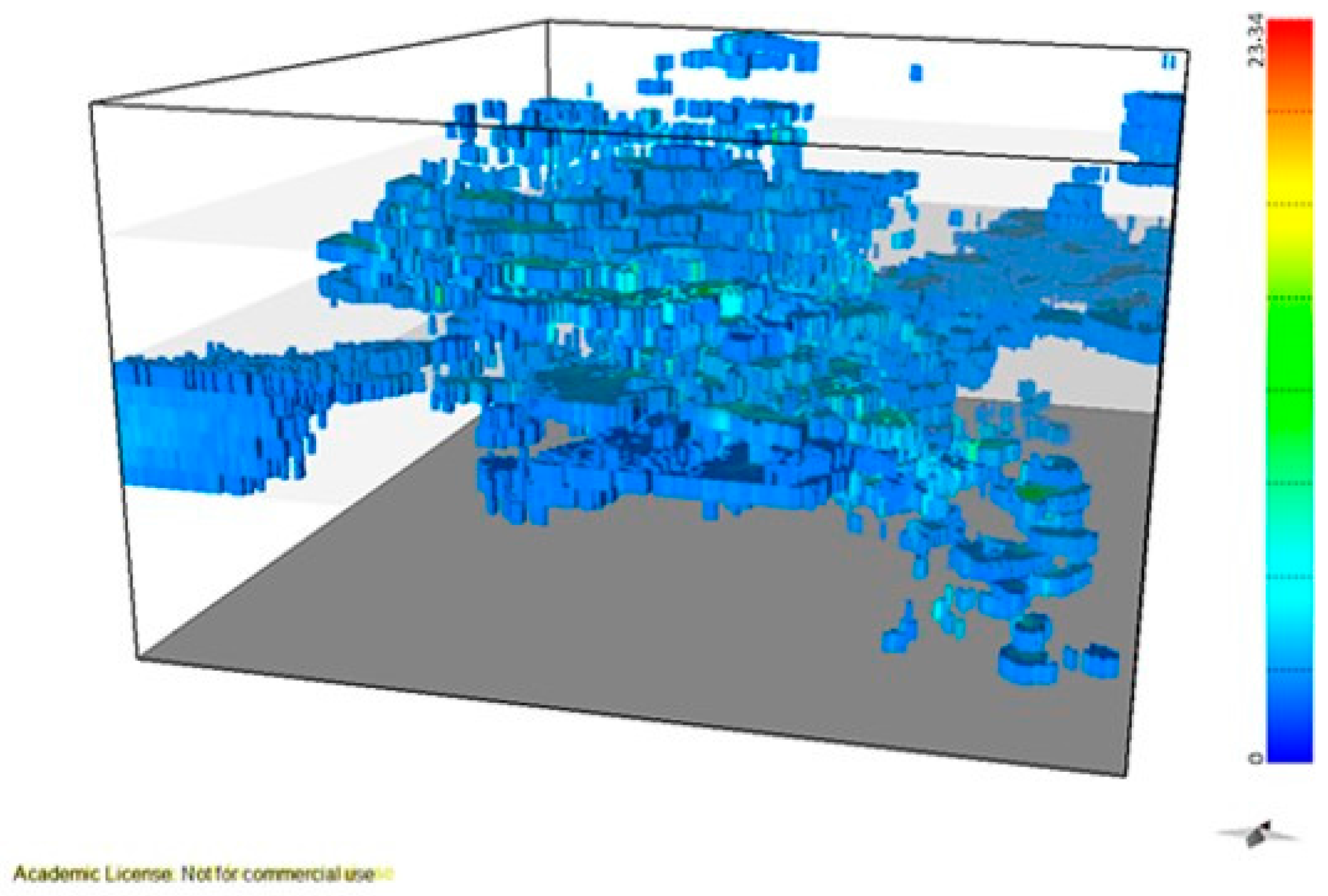
Equation (11) allowed the WQ in kilograms (or tons) to be determined for each model cell for the 1000 scenarios. Then, each scenario was vertically upscaled to the 10 m × 10 m × 10 m grid, and maps of the average quantity (kg) and CV were produced (Figure 16).
An inspection of the average mineral potential map shows that the richest wolframite zones occur in levels L1 and L2 and that they are distributed mostly within the central part of the model. This means that in these zones, high quantities of wolframite (kg/m3) and high values of VP occur together. The map of the CV is consistent with the patterns seen in the morphology and wolframite content models.
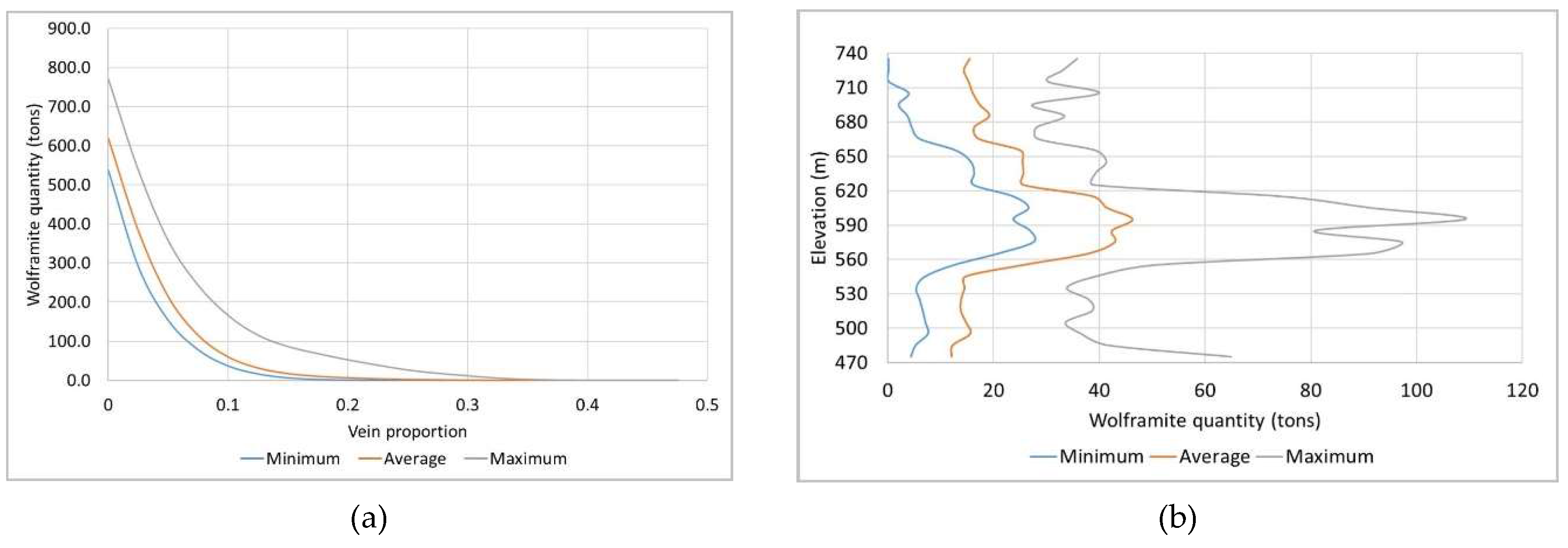
The maps of WQ show the average mineral potential for the whole deposit and by mine level, as well as assigning uncertainty ranges. The presented maps do not exclude the amounts already exploited; that is, they consider the deposit as being non-exploited. Figure 17a and b display the cumulative WQ (tons) as a function of VP and the cumulative WQ (tons) as a function of the elevation, respectively. These graphs show the optimistic curve (best simulated scenario), the pessimistic curve (worst simulated scenario), and the average curve of the simulations.
Figure 17a shows that the estimated average mineral potential of the deposit is 618.47 tons, with the optimistic scenario being 769.73 tons and the pessimistic scenario being 537.19 tons. It should be noted that the presented values do not consider the exploited volumes, nor do they represent actual values, as they are proportional to WQ standardized to [0, 1] (for reasons of confidentiality). The mineral potential curves by elevation (Figure 17b) indicate that the mine level with the highest estimated potential is L2, confirming the result of the wolframite content modelling in section 3.4.5. The variability in WQ is high over the entire vertical extent of the mine, although with somewhat lower values at the L1–L2 and L2–L3 interfaces. Figure 18 presents the 3D visualization of the average mineral potential using a 10 m × 10 m × 10 m grid.
4. Discussion
The presented methodology integrates all the available data, from both stopes and boreholes, and takes into consideration the particular characteristics of the data, namely, the different sampling methods and distinct spatial biases. These data characteristics made it unfeasible to use conventional non-geostatistical methods to model the deposit, meaning that an optimized methodology had to be developed in order to combine all the data and to avoid bias.
An initial overview of the problem showed that the greatest challenge in defining a methodology for modelling the deposit was to adjust the methods to the data and sampling characteristics, namely: the different data sources and sampling patterns; which information or data source should be defined as primary; which data source better represents the distributional behavior of the variables; the sampling and data biases; the data types (continuous and categorical); and the adaption of traditional geostatistical methods to the problem.
Geostatistical methods for estimation did not correspond to the requirements imposed by the data and sampling, as they did not allow combining large amounts of information, divided into primary and secondary information, and in different sampling patterns and sizes, characteristics that assumed an important role in the interpretation of the results. Therefore, we used stochastic simulation, whose algorithms are easily modified and adapted to the needs of the problem and which allow the local uncertainty to be quantified through the samples’ proximity and heterogeneity.
The proposed methodology considered all the presented conditions, allowing two independent models to be built, namely, models of morphology and wolframite content, which were subsequently crossed to quantify the mineral potential in each model cell (10 m × 10 m × 10 m). The available information was integrated into the models as hard data (stopes) and as soft data (boreholes).
The integration of some data as soft data into the methodology developed was shown to be valid and efficient because it allowed a model to be created that was conditioned to the spatial structure and statistics of the boreholes, which are considered more representative of the volume compared with the stopes. Although borehole data are less abundant than stope data in some parts of the deposit, these soft data are globally less skewed than the stope data, so they better represent the true behavior of the property of interest (VP).
The univariate statistical analysis of the variables showed the following: (i) There is an obvious sampling bias, with the stope average VP being seven times greater than the borehole average VP; (ii) mine levels L1 and L2 are the richest in wolframite; and (iii) the majority of borehole modal WQ measurements belong to classes 0 and 1, representing low wolframite contents.
The high bias identified in the stope-derived VP variable can be explained in terms of the fact that stoping operations follow the presence of veins. On the other hand, the sampling in the boreholes is conducted continuously along/down each borehole, meaning that the data are close to reality.
An initial study of the stope and borehole vein proportion variables helped to establish that the VP simulation needs to be conditioned to the stope data (hard data) and the spatial structure of those data, to the ungrouped borehole statistics, and to the borehole data, as local means in a 50 m × 50 m × 30 m grid (soft data).
The final morphology model allows the following conclusions to be made: (i) The thickest zone of the deposit is found in the central part of the modelled region, corresponding to levels L1 and L2; (ii) The local uncertainty is higher in the peripheral parts of the modelled deposit, as expected, and zero in the stope location. There are some local high values of CV, explained in terms of the occurrence of very dissimilar values in close proximity within zones of high sampling density; and (iii) The adjustments to output variograms in the different phases of the methodology present a discrepancy because the application of the correction of averages (in step 3) increases the data variance, distorting the variograms.
The VP data are concentrated in the central part of the model. The simulation extends beyond the stope data where the borehole-derived data exhibit low or null values, so the methodology simulates values that, in these peripheral parts of the model, tend to be lower.
Contrary to the initial information of the morphology model, the WQ variables are distinct, being continuous in stopes and modal in boreholes, and it was necessary to formulate an appropriate methodology, establishing the objective of simulating WQ conditioned to the data measured in stopes (hard data) and to the wolframite classes reported in boreholes (soft data).
The primary and secondary data are not co-located, so it was necessary to cross the information by proximity. As there were too many borehole wolframite classes with poor discrimination, the seven classes were grouped into two classes, corresponding to low quantity, CL1 {0, 1, 2}, and to high quantity, CL2 {3, 4, 5, 6}, for each of the four mine levels. The discrimination of the classes is reasonable in levels L0 and L3 and non-existent in levels L1 and L2.
The simulated WQ variograms are similar to the variograms for the initial data, with small discrepancies because the WQ variograms are calculated and adjusted for the total data set and the WQ simulation is conditional to CL1 and CL2 and uses split data sets. The simulation also influences the final statistics, as the probability of belonging to each class estimation has a degradational effect in the data that is more pronounced in the peripheral zones of the model, where the stope wolframite quantities are lower, generating more accentuated left-skewed distribution laws.
By conditioning the WQ simulation to histograms by mine level, the results are more consistent, mainly because many of the simulated regions are located far from stopes and there is a clear segregation of WQ with depth.
The final wolframite content model allows the following conclusions to be made: (i) The richest part of the modelled deposit corresponds to level L2, followed by L1. (ii) The model uncertainty behavior is similar to that of the morphology model. However, a region of high dispersion is evident in level L2 (in the southwestern part of the deposit), where wide discrepancies exist between neighboring values, forcing the simulation to generate different values between each scenario.
Finally, crossing the two independent models allowed the wolframite resource to be quantified. The results show that: (i) The richest part of the modelled deposit corresponds to levels L1 and L2 (the central part of the model); (ii) the estimated mineral potential of the deposit is 618.47 tons, with the optimistic scenario being 769.73 tons and the pessimistic scenario being 537.19 tons; and (iii) the variation in WQ by elevation indicates that the richest level is L2, supporting the interpretations of the wolframite content model.
Although the proposed methodology involves many steps and combinations of results, this study has shown that the implementation of the methodology to a deposit being mined is feasible and does not require huge computational effort, if the proposed procedures are chained as scripts. DSS simulations are quick procedures and depend only on the total number of cells of the model and the amount of available data. To give an idea of the computational effort, the DSS of a variable in the higher-resolution grid used in this study, involving almost 5 million blocks, represents about two minutes of computation per realization using a computer with an Intel® I7 processor.
5. Conclusions
This study is based on a decades-long exploited mineral vein deposit, with a unique pattern of sampling and data collection, where the problem is how to appropriately handle and analyze a large volume of data according to their various characteristics. The objective of this study was to establish a methodology for building a 3D geological model of a mineral vein deposit, combining stope data (vein thickness and wolframite quantity, WQ) and borehole data (vein thickness and wolframite modal classes).
The approach formulated here considered the initially identified sampling and data issues, allowing two independent models to be created, namely, a morphology model and a wolframite content model. All available information, comprising hard data (from stopes) and soft data (from boreholes), was used to build the models. As a final outcome, the potential of the mineral deposit was quantified by integrating the results of the two methodologies.
In the morphological model, the application of two-phase DSS is an innovative approach. Although the stope variograms are of high quality, the borehole data had to be declustered on a 50 m × 50 m × 30 m grid, being used as local means. The application of the methodology allowed us to conclude that zones of thicker mineral veins coincide with mine levels L1 and L2. In the model of wolframite quantity, the information from stopes and boreholes is not co-located, so a proximity study had to be conducted. The poor discrimination of WQ by borehole modal quantity classes revealed the need to group the classes. By crossing the two independent models, it was possible to quantify the mineral potential of the deposit, revealing that the richest zone corresponds to the central parts of the deposit.
The methodology proved to be very suitable for integrating data from different sources, namely, stopes and boreholes, and with distinct spatial biases. However, future work could include reviewing the borehole database, incorporating the local means correction into the DSS algorithm, and studying WQ in a more closely defined and smaller part of the deposit.
Acknowledgments
A.S. acknowledges the Fundação para a Ciência e Tecnologia (FCT), Portugal, for Grant SFRH/BD/117613/2016. The authors are grateful to Midland Valley for providing an academic license for Move® software. This work is a contribution to Project UID/GEO/04035/2013 funded by FCT - Fundação para a Ciência e a Tecnologia, in Portugal.
Author Contributions
A.S. and J.A. conceived, designed, and performed the experiments; all authors analyzed the data; J.A. and P.C. revised the methodology; R.V. revised the geology and mineral deposit settings; J.A. and R.V. contributed documents, materials, and analysis tools; A.S. wrote the paper.
Conflicts of Interest
The authors declare no conflict of interest. It should be noted that the wolframite quantities and consequent results are standardized to the interval [0, 1] and the coordinates translated to the point (0, 0, 470) m, for reasons of confidentiality.
Appendix A.—Methodology Flowcharts
Figure A1.
Morphology methodology flowchart.

Figure A2.
Wolframite content methodology flowchart.

Appendix B.—Univariate Statistical Analysis

Table A1.
Stope vein thickness statistics.
| Parameters | L0 | L1 | L2 | L3 | Global |
|---|---|---|---|---|---|
| No samples | 3425 | 21,635 | 31,581 | 2333 | 59,047 |
| Average | 26.7 | 30.7 | 32.4 | 34.3 | 31.5 |
| Variance | 103.24 | 222.72 | 177.12 | 306.44 | 197.27 |
| Coefficient of variation | 0.38 | 0.49 | 0.41 | 0.51 | 0.45 |
| Minimum | 0.0 | 0.0 | 0.0 | 0.0 | 0.0 |
| Q1 | 19.5 | 20.0 | 24.0 | 21.0 | 21.5 |
| Medium | 26.0 | 30.0 | 33.0 | 31.0 | 31.0 |
| Q3 | 32.5 | 37.0 | 40.0 | 45.5 | 39.0 |
| Maximum | 73.0 | 126.0 | 82.0 | 105.0 | 126.0 |
| Skewness coefficient | 0.64 | 1.20 | 0.36 | 0.80 | 0.79 |
Table A2.
Stope vein proportion statistics.
| Parameters | L0 | L1 | L2 | L3 | Global |
|---|---|---|---|---|---|
| No samples | 3425 | 21,635 | 31,581 | 2333 | 59,047 |
| Average | 0.121 | 0.139 | 0.147 | 0.156 | 0.143 |
| Variance | 0.002 | 0.005 | 0.004 | 0.006 | 0.004 |
| Coefficient of variation | 0.381 | 0.486 | 0.411 | 0.511 | 0.445 |
| Minimum | 0.000 | 0.000 | 0.000 | 0.000 | 0.000 |
| Q1 | 0.089 | 0.091 | 0.109 | 0.095 | 0.098 |
| Medium | 0.118 | 0.136 | 0.150 | 0.141 | 0.141 |
| Q3 | 0.148 | 0.168 | 0.182 | 0.207 | 0.177 |
| Maximum | 0.332 | 0.573 | 0.373 | 0.477 | 0.573 |
| Skewness coefficient | 0.637 | 1.199 | 0.359 | 0.804 | 0.786 |
Table A3.
Stope wolframite quantity statistics.
| Parameters | L0 | L1 | L2 | L3 | Global |
|---|---|---|---|---|---|
| No samples | 3425 | 21,635 | 31,581 | 2406 | 59,047 |
| Average | 0.028 | 0.038 | 0.054 | 0.033 | 0.046 |
| Variance | 0.001 | 0.001 | 0.001 | 0.002 | 0.001 |
| Coefficient of variation | 1.182 | 0.854 | 0.675 | 1.198 | 0.789 |
| Minimum | 0.0 | 0.0 | 0.0 | 0.0 | 0.0 |
| Q1 | 0.007 | 0.013 | 0.026 | 0.001 | 0.016 |
| Medium | 0.018 | 0.035 | 0.057 | 0.023 | 0.046 |
| Q3 | 0.037 | 0.057 | 0.075 | 0.050 | 0.069 |
| Maximum | 0.329 | 0.608 | 1.000 | 0.418 | 1.000 |
| Skewness coefficient | 2.95 | 2.70 | 2.45 | 2.66 | 2.38 |
Table A4.
Borehole vein thickness statistics.
| Parameters | L0 | L1 | L2 | L3 | Global |
|---|---|---|---|---|---|
| No samples | 2615 | 7022 | 7846 | 3509 | 20,992 |
| Average | 9.0 | 10.9 | 12.7 | 13.1 | 11.7 |
| Variance | 80.0 | 146.3 | 192.8 | 193.8 | 165.2 |
| Coefficient of variation | 0.997 | 1.107 | 1.090 | 1.065 | 1.097 |
| Minimum | 1 | 1 | 1 | 1 | 1 |
| Q1 | 3 | 4 | 5 | 4 | 4 |
| Medium | 6 | 7 | 8 | 8 | 8 |
| Q3 | 12 | 14 | 16 | 17 | 15 |
| Maximum | 78 | 190 | 160 | 174 | 190 |
| Skewness coefficient | 2.26 | 3.43 | 2.94 | 2.46 | 3.03 |
Table A5.
Borehole vein proportion statistics.
| Parameters | L0 | L1 | L2 | L3 | Global |
|---|---|---|---|---|---|
| No samples | 340 | 638 | 710 | 521 | 2209 |
| Average | 0.022 | 0.026 | 0.021 | 0.015 | 0.021 |
| Variance | 0.0002 | 0.0004 | 0.0002 | 0.0002 | 0.0003 |
| Coefficient of variation | 0.683 | 0.746 | 0.649 | 0.860 | 0.757 |
| Minimum | 0.000 | 0.000 | 0.000 | 0.000 | 0.000 |
| Q1 | 0.011 | 0.012 | 0.011 | 0.004 | 0.009 |
| Medium | 0.020 | 0.022 | 0.020 | 0.011 | 0.018 |
| Q3 | 0.030 | 0.036 | 0.030 | 0.022 | 0.030 |
| Maximum | 0.096 | 0.109 | 0.081 | 0.060 | 0.109 |
| Skewness coefficient | 0.992 | 1.187 | 0.736 | 0.958 | 1.178 |
Table A6.
Borehole wolframite modal quantity statistics.
| Level | Class | No Veins | % | Total Thick. (cm) | Average Thick. (cm) |
|---|---|---|---|---|---|
| Global | 0 | 16,261 | 80.8% | 168,839.0 | 10.4 |
| 1 | 2009 | 10.0% | 31,278.6 | 15.6 | |
| 2 | 642 | 3.2% | 10,279.5 | 16.0 | |
| 3 | 610 | 3.0% | 10,018.5 | 16.4 | |
| 4 | 409 | 2.0% | 7434.5 | 18.2 | |
| 5 | 158 | 0.8% | 2952.5 | 18.7 | |
| 6 | 42 | 0.2% | 677.0 | 16.1 | |
| Total | 20,131 | 231,479.6 | 11.5 | ||
| L0 | 0 | 2041 | 84.5% | 15,919.5 | 7.8 |
| 1 | 300 | 12.4% | 3400.0 | 11.3 | |
| 2 | 33 | 1.4% | 383.0 | 11.6 | |
| 3 | 18 | 0.7% | 316.0 | 17.6 | |
| 4 | 12 | 0.5% | 200.0 | 16.7 | |
| 5 | 9 | 0.4% | 93.0 | 10.3 | |
| 6 | 2 | 0.1% | 21.0 | 10.5 | |
| Total | 2415 | 20,332.5 | 8.4 | ||
| L1 | 0 | 5212 | 81.7% | 47,952.5 | 9.2 |
| 1 | 711 | 11.1% | 10,652.1 | 15.0 | |
| 2 | 114 | 1.8% | 1644.0 | 14.4 | |
| 3 | 162 | 2.5% | 2508.5 | 15.5 | |
| 4 | 120 | 1.9% | 1856.0 | 15.5 | |
| 5 | 47 | 0.7% | 826.0 | 17.6 | |
| 6 | 14 | 0.2% | 271.0 | 19.4 | |
| Total | 6380 | 65,710.1 | 10.3 | ||
| L2 | 0 | 6182 | 79.0% | 70,648.0 | 11.4 |
| 1 | 755 | 9.6% | 13,441.0 | 17.8 | |
| 2 | 315 | 4.0% | 5124.5 | 16.3 | |
| 3 | 295 | 3.8% | 4735.0 | 16.1 | |
| 4 | 206 | 2.6% | 4078.5 | 19.8 | |
| 5 | 64 | 0.8% | 1393.5 | 21.8 | |
| 6 | 13 | 0.2% | 186.0 | 14.3 | |
| Total | 7830 | 99,606.5 | 12.7 | ||
| L3 | 0 | 2826 | 80.6% | 34,293.0 | 12.1 |
| 1 | 243 | 6.9% | 3785.5 | 15.6 | |
| 2 | 180 | 5.1% | 3128.0 | 17.4 | |
| 3 | 135 | 3.9% | 2459.0 | 18.2 | |
| 4 | 71 | 2.0% | 1300.0 | 18.3 | |
| 5 | 38 | 1.1% | 640.0 | 16.8 | |
| 6 | 13 | 0.4% | 199.0 | 15.3 | |
| Total | 3506 | 45,804.5 | 13.1 | ||
Figure A3.
Cumulative histograms for stope variables: (a) Vein thickness, (b) vein proportion, and (c) wolframite quantity.
Figure A3.
Cumulative histograms for stope variables: (a) Vein thickness, (b) vein proportion, and (c) wolframite quantity.

Figure A4.
Cumulative histograms for borehole variables: (a) Vein thickness and (b) vein proportion.
Figure A4.
Cumulative histograms for borehole variables: (a) Vein thickness and (b) vein proportion.
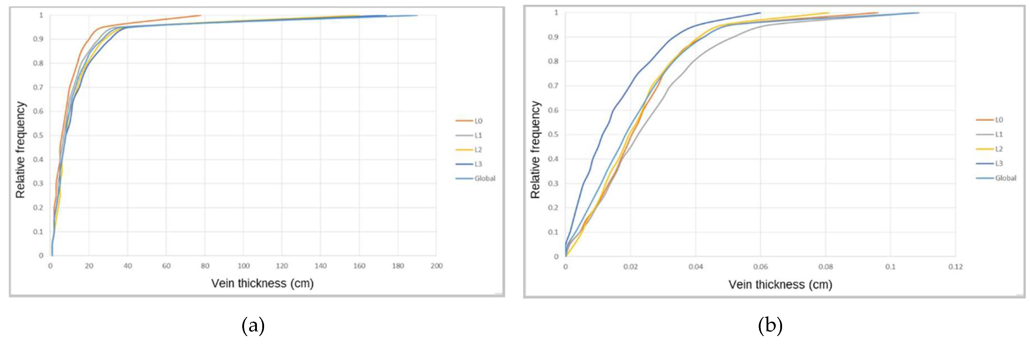
Figure A5.
Borehole wolframite modal quantity histograms: (a) L0, (b) L1, (c) L2, (d) L3, and (e) global.
Figure A5.
Borehole wolframite modal quantity histograms: (a) L0, (b) L1, (c) L2, (d) L3, and (e) global.

Appendix C.—Morphology Model Supplementary Content
Figure A6.
Borehole VP omnidirectional variograms: (a) borehole data regularization performed on a 10 m × 10 m × 10 m grid; (b) borehole data regularization performed on a 20 m × 20 m × 20 m grid.
Figure A6.
Borehole VP omnidirectional variograms: (a) borehole data regularization performed on a 10 m × 10 m × 10 m grid; (b) borehole data regularization performed on a 20 m × 20 m × 20 m grid.

Table A7.
Calculation and adjustment parameters for borehole VP variograms.
| Variogram Calculation | ||||||
|---|---|---|---|---|---|---|
| Direction (Azimuth, Dip) | Tolerance | Lag | Horizontal Variogram | |||
| (0, 0) | 180 | 50 | 25 | |||
| (0, 90) | 5 | 30 | - | |||
| Theoretical Model Adjustment | ||||||
| Direction (Azimuth, Dip) | C0 | Model | C1 | A1 | C2 | A2 |
| (0, 0) | 0 | Exponential | 1 | 350 | - | - |
| (0, 90) | 0 | Exponential | 1 | 170 | - | - |
Figure A7.
Borehole VP directional variograms: (a) horizontal variogram; (b) vertical variogram. The regularization was performed on a 50 m × 50 m × 30 m grid.
Figure A7.
Borehole VP directional variograms: (a) horizontal variogram; (b) vertical variogram. The regularization was performed on a 50 m × 50 m × 30 m grid.
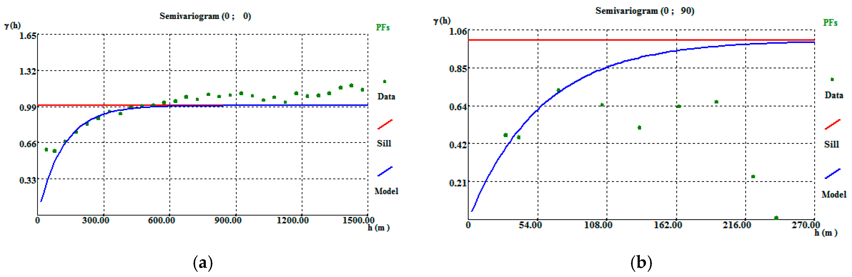
Table A8.
Calculation and adjustment parameters for stope VP variograms.
| Variogram Calculation | ||||||
|---|---|---|---|---|---|---|
| Direction (Azimuth, Dip) | Tolerance | Lag | Horizontal Variogram | |||
| (30, 0) | 45 | 20 | 5 | |||
| (−60, 0) | 45 | 20 | 5 | |||
| (0, 90) | 5 | 32 | - | |||
| Theoretical Model Adjustment | ||||||
| Direction (Azimuth, Dip) | C0 | Model | C1 | A1 | C2 | A2 |
| (30, 0) | 0 | Exponential | 1 | 600 | - | - |
| (−60, 0) | 0 | Exponential | 1 | 600 | - | - |
| (0, 90) | 0 | Exponential | 1 | 40 | - | - |
Figure A8.
Stope vein proportion directional variograms: (a) horizontal (30, 0) variogram; (b) horizontal (−60, 0) variogram; and (c) vertical variogram. The stope data were declustered on a 10 m × 10 m × 2 m grid.
Figure A8.
Stope vein proportion directional variograms: (a) horizontal (30, 0) variogram; (b) horizontal (−60, 0) variogram; and (c) vertical variogram. The stope data were declustered on a 10 m × 10 m × 2 m grid.
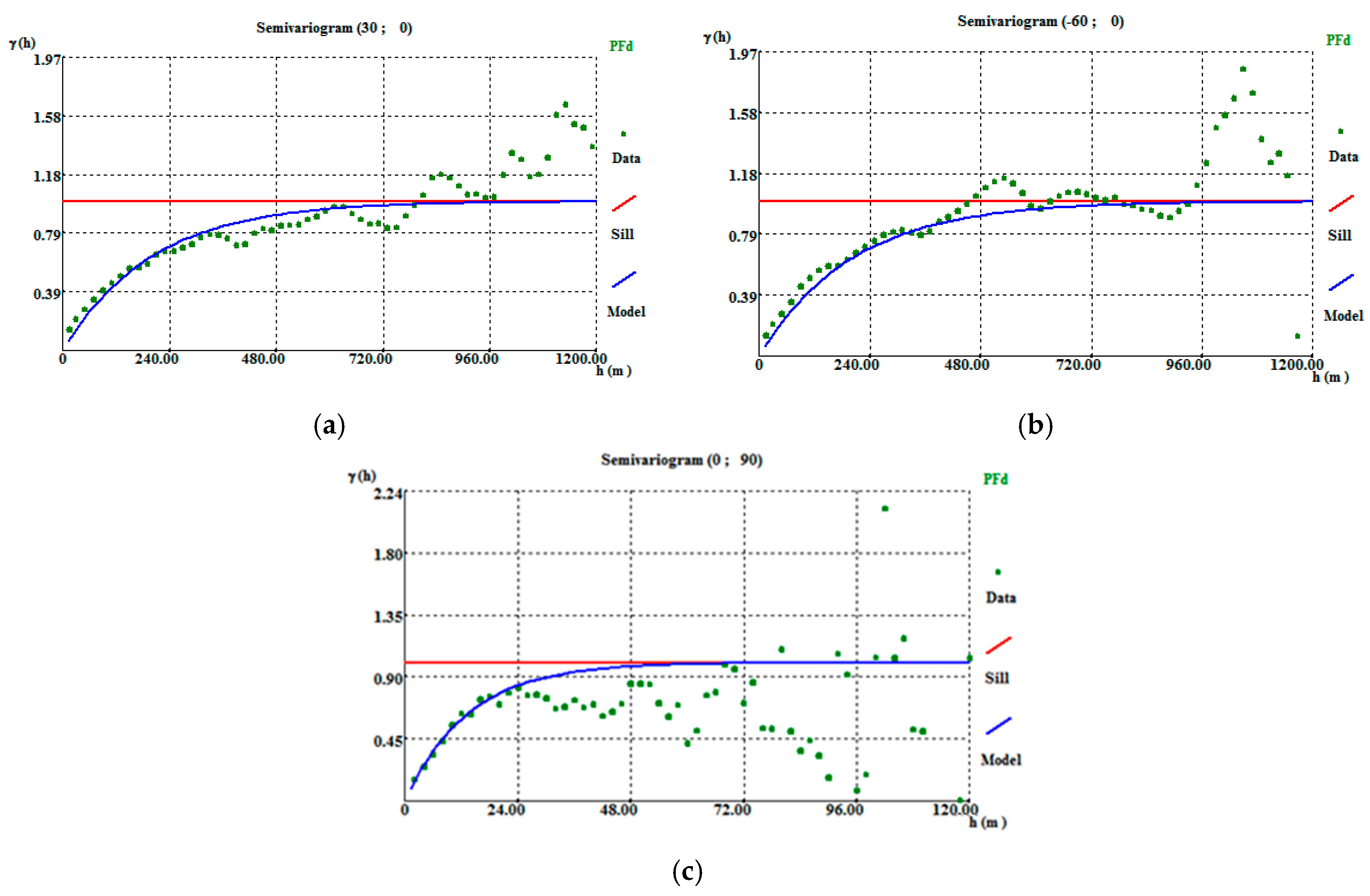
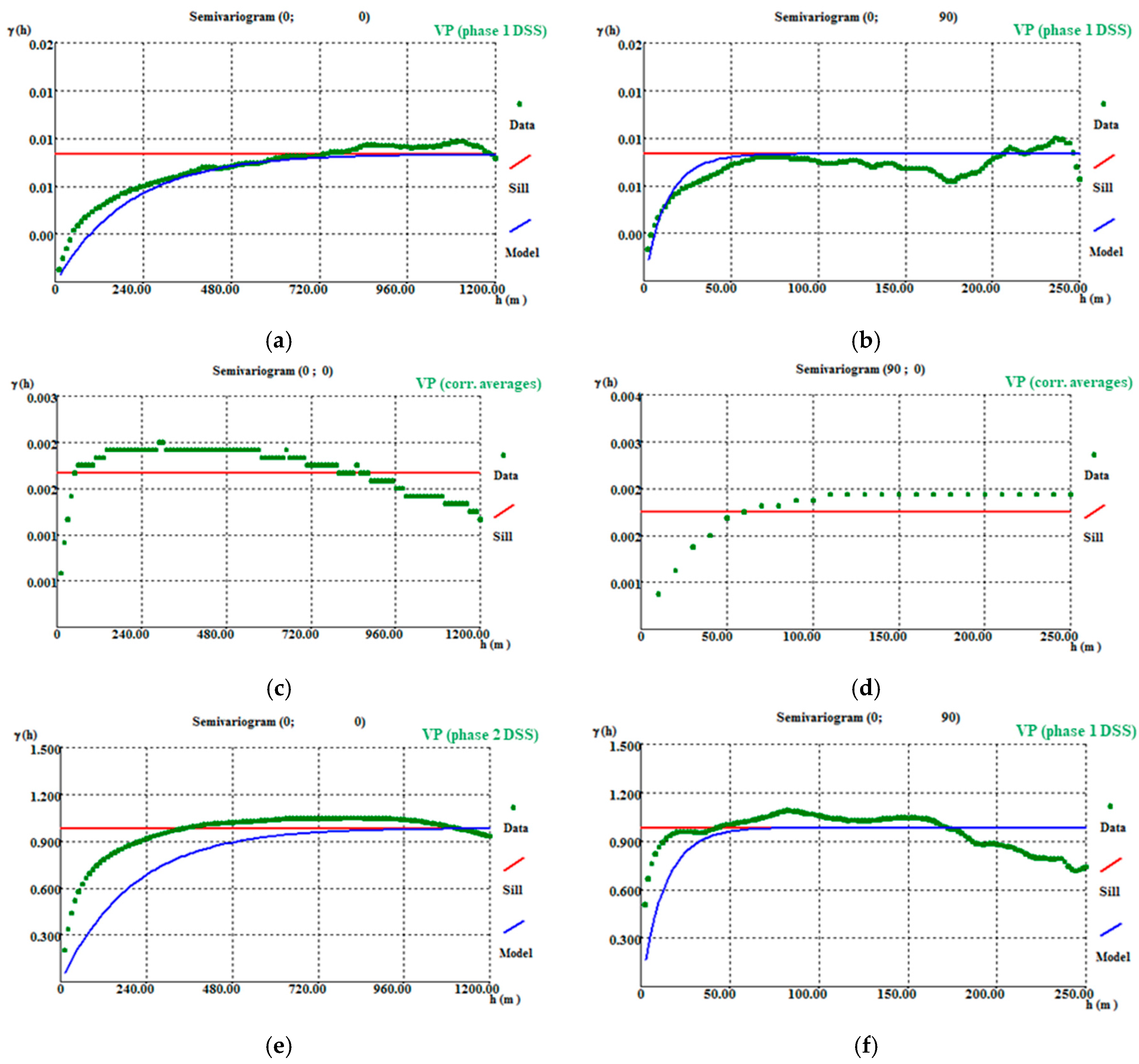
Figure A9.
Different phases of variogram adjustment applied to the first simulated scenario: (a) DSS phase 1 horizontal variogram; (b) DSS phase 1 vertical variogram; (c) DSS phase 1 average correction horizontal variogram; (d) DSS phase 1 average correction vertical variogram; (e) DSS phase 2 horizontal variogram; (f) DSS phase 2 vertical variogram.
Appendix D.—Wolframite Content Model Supplementary Content
Table A9.
Calculation and adjustment parameters for the borehole CL1 indicator variable variograms.
| Variogram Calculation | ||||||
|---|---|---|---|---|---|---|
| Direction (Azimuth, Dip) | Tolerance | Lag | Horizontal Variogram | |||
| (0, 0) | 180 | 50 | 25 | |||
| (0, 90) | 5 | 30 | - | |||
| Theoretical Model Adjustment | ||||||
| Direction (Azimuth, Dip) | C0 | Model | C1 | A1 | C2 | A2 |
| (0, 0) | 0 | Exponential | 1 | 70 | - | - |
| (0, 90) | 0 | Exponential | 1 | 50 | - | - |
Figure A10.
Borehole CL1 indicator variable directional variograms: (a) horizontal variogram and (b) vertical variogram. On a 50 m × 50 m × 30 m grid.
Figure A10.
Borehole CL1 indicator variable directional variograms: (a) horizontal variogram and (b) vertical variogram. On a 50 m × 50 m × 30 m grid.
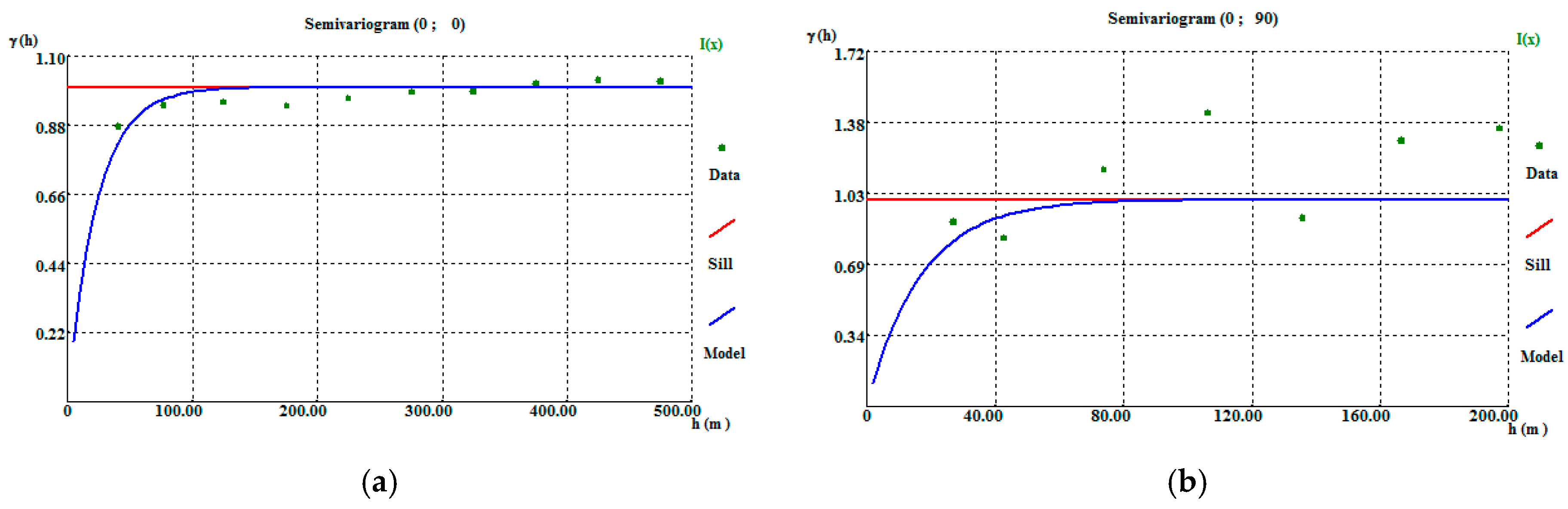
Table A10.
Calculation and adjustment parameters for the stope vein proportion variograms.
| Variogram Calculation | ||||||
|---|---|---|---|---|---|---|
| Direction (Azimuth, Dip) | Tolerance | Lag | Horizontal Variogram | |||
| (0, 0) | 180 | 10 | 1 | |||
| (0, 90) | 5 | 8 | - | |||
| Theoretical Model Adjustment | ||||||
| Direction (Azimuth, Dip) | C0 | Model | C1 | A1 | C2 | A2 |
| (0, 0) | 0.3 | Spherical | 0.7 | 500 | - | - |
| (0, 90) | 0.3 | Spherical | 0.7 | 60 | - | - |
Figure A11.
Stope wolframite quantity (kg/m3) directional variograms: (a) horizontal omnidirectional variogram and (b) vertical variogram. On a 10 m × 10 m × 2 m grid.
Figure A11.
Stope wolframite quantity (kg/m3) directional variograms: (a) horizontal omnidirectional variogram and (b) vertical variogram. On a 10 m × 10 m × 2 m grid.
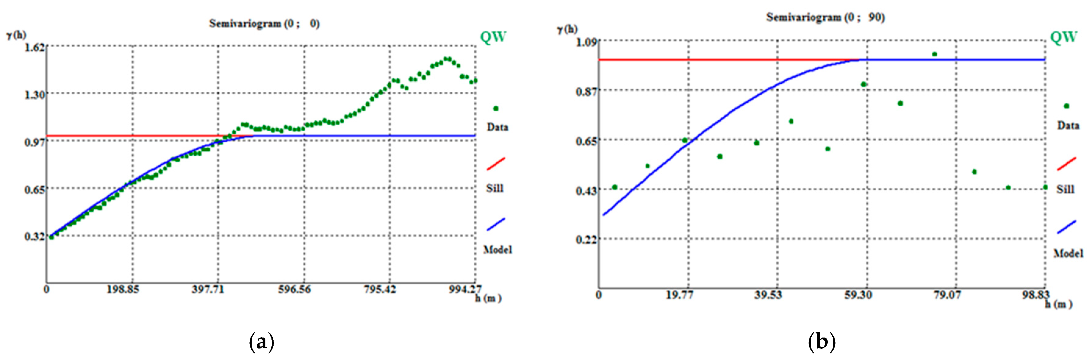
Figure A12.
Step 3 DSS output variogram adjustment applied to the first simulated scenario: (a) CL1 DSS horizontal variogram; (b) CL1 DSS vertical variogram; (c) CL2 DSS horizontal variogram; (d) CL2 DSS vertical variogram.
Figure A12.
Step 3 DSS output variogram adjustment applied to the first simulated scenario: (a) CL1 DSS horizontal variogram; (b) CL1 DSS vertical variogram; (c) CL2 DSS horizontal variogram; (d) CL2 DSS vertical variogram.
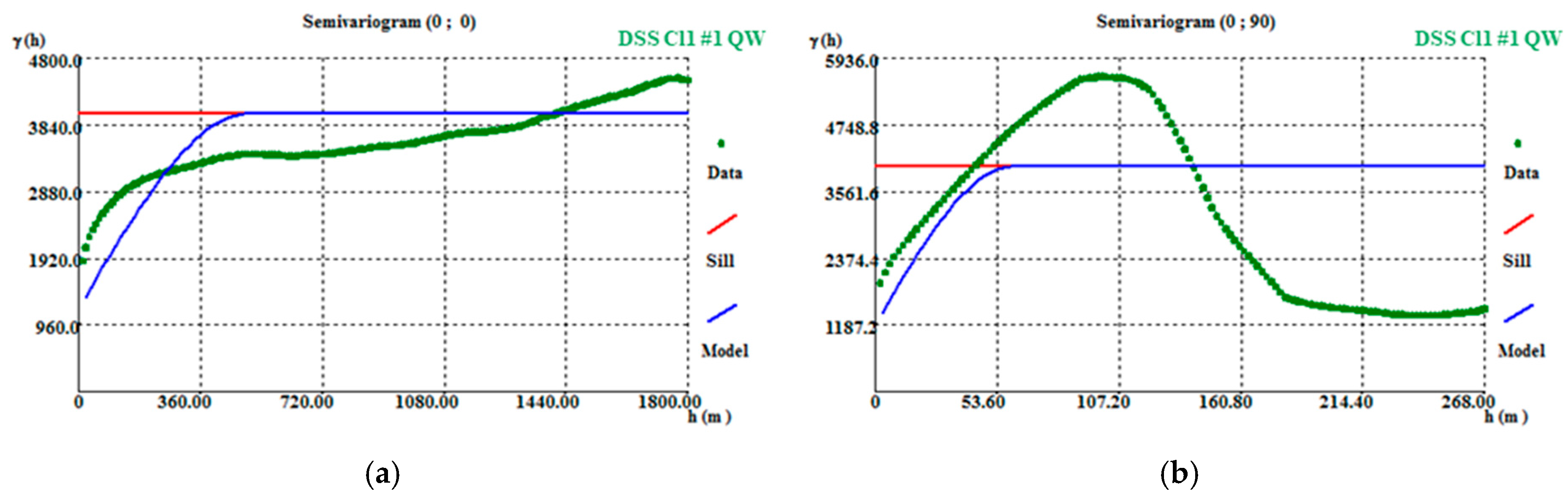

Table A11.
Wolframite quantity statistical analysis comparison—initial data set and Probability Field Simulation first scenario.
Table A11.
Wolframite quantity statistical analysis comparison—initial data set and Probability Field Simulation first scenario.
| Parameters | INITIAL DATA | PFS 1 |
|---|---|---|
| No samples | 59,047 | 4,819,500 |
| Average | 0.046 | 0.045 |
| Variance | 0.001 | 0.004 |
| Standard deviation | 0.036 | 0.063 |
| Coefficient of variation | 0.79 | 1.37 |
| Minimum | 0.00 | 0.00 |
| Q1 | 0.016 | 0.01 |
| Medium | 0.046 | 0.03 |
| Q3 | 0.069 | 0.057 |
| Maximum | 1 | 0.98 |
| Skewness coefficient | 2.38 | 4.429 |
References
- European Commission. Report on Critical Raw Materials for the EU, Report of the Ad Hoc Working Group on Defining Critical Raw Materials; European Commission: Brussels, Belgium, 2014; p. 41. [Google Scholar]
- Simões, T. Modelação Automática 2D de Mineralizações Filonianas—Aplicação às Minas da Panasqueira. Master’s Thesis, Science and Technology Faculty of NOVA University of Lisbon, Almada, Portugal, 2014. [Google Scholar]
- Soares, A. Geostatística para as Ciências da Terra e do Ambiente, 3rd ed.; ISTPress: Lisboa, Portugal, 2014; p. 232. ISBN 978-972-8469-46-7. [Google Scholar]
- Charifo, A.; Almeida, J.A.; Ferreira, A. Managing borehole samples of unequal lengths to construct a high-resolution mining model of mineral grades zoned by geological units. JGE 2013, 132, 209–223. [Google Scholar] [CrossRef]
- Neiva, J. Jazigos Portugueses de Cassiterite e de Volframite. In Comunicações dos Serviços Geológicos de Portugal, Tomo XXV, 1st ed.; Direcção Geral de Minas e Serviços Geológicos: Lisbon, Portugal, 1944; Volume 25, p. 251. [Google Scholar]
- Conde, L.; Pereira, V.; Ribeiro, A.; Thadeu, D. Jazigos hipogénicos de estanho e volfrâmio. In Livro-Guia da Excursão: I Congresso Hispano-Luso-Americano de Geologia Económica, 1st ed.; Direcção Geral de Minas e Serviços Geológicos: Lisbon, Portugal, 1971; Volume 7, p. 81. [Google Scholar]
- Noronha, F. Jazigos filonianos hidrotermais de estanho e volfrâmio. Considerações acerca da sua génese. In Proceedings of the 1° Colóquio de Jazigos Minerais Metálicos de Portugal, Lisbon, Portugal, 26 October 1999; Academia das Ciências de Lisboa: Lisbon, Portugal, 1999; pp. 1–19. [Google Scholar]
- Thadeu, D. Le gisement stanno-wolframifère de Panasqueira (Portugal). In Chronique De La Recherche Minière, 1st ed.; Bureau de Recherches Géologiques et Minières: Paris, France, 1979; Volume 450, pp. 35–42. [Google Scholar]
- Thadeu, D. Geologia do Couto Mineiro da Panasqueira. In Comunicações dos Serviços Geológicos de Portugal, Tomo XXXII, 1st ed.; Direcção Geral de Minas e Serviços Geológicos: Lisbon, Portugal, 1951; Volume 32, p. 64. [Google Scholar]
- Ribeiro, A.; Pereira, E. Controles paleogeográficos, petrológicos e estruturais na génese dos jazigos portugueses de estanho e volfrâmio. Geonovas 1982, 1, 23–31. [Google Scholar]
- Williams, C. Ore Estimation and Mine Planning at Panasqueira, Portugal. Ph.D. Thesis, Royal School of Mines, London, UK, 1985. [Google Scholar]
- Kelly, W.C.; Rye, R.O. Geologic, fluid inclusion, and stable isotope studies of the tin-tungsten deposits of Panasqueira, Portugal. Econ. Geol. 1979, 74, 1721–1822. [Google Scholar] [CrossRef]
- Pinto, F. Estudo da distribuição do Estanho na Mina da Panasqueira. Master’s Thesis, Science Faculty of University of Porto, Porto, Portugal, 2014. [Google Scholar]
- Franco, A.; Vieira, R.; Bunting, R. The Panasqueira Mine at a Glance—Tungsten Newsletter; ITIA: London, UK, 2014; p. 16. [Google Scholar]
- Rossi, M.; Deutsch, C. Mineral Resource Estimation, 1st ed.; Springer: Dordrecht, The Netherland, 2014; p. 332. ISBN 978-1-4020-5717-5. [Google Scholar]
- Goovaerts, P. Geostatistics for Natural Resources Evaluation, 1st ed.; Oxford University Press: New York, NY, USA, 1997; p. 483. ISBN 978-0-19-511538-4. [Google Scholar]
- Rodrigues, A. Modelação 3D de Teores de Depósitos Minerais Condicionados por tipos de Mineralização: O Caso de Estudo do Depósito Mineral do Zambujal, Minas de Neves-Corvo. Master’s Thesis, Science and Technology Faculty of NOVA University of Lisbon, Almada, Portugal, 2013. [Google Scholar]
- Silva, D.; Almeida, J.A. The use of rock density for improving morphological and metal grade models of the Zambujal sulphide ore deposit (Neves–Corvo Mine). In Proceedings of the 17th Annual Conference of the IAMG, Freiberg, Germany, 23 June 2015. [Google Scholar]
- Almeida, J. Modelling of cement raw material compositional indices with direct sequential simulation. Eng. Geol. 2010, 114, 26–33. [Google Scholar] [CrossRef]
- Matias, F.; Almeida, J.; Chichorro, M. A Multistep Methodology for Building a Stochastic Model of Gold Grades in the Disseminated and Complex Deposit of Casas Novas in Alentejo, Southern Portugal. Resour. Geol. 2015, 65, 361–374. [Google Scholar] [CrossRef]
- Soares, A. Direct Sequential Simulation and Cosimulation. Math. Geol. 2001, 33, 911–926. [Google Scholar] [CrossRef]
- Srivastava, R.; Froidevaux, R. Probability Field Simulation: A Retrospective. In Quantitative Geology and Geostatistics, 1st ed.; Springer: Dordrecht, The Netherlands, 2004; Volume 14, pp. 55–64. ISBN 978-1-4020-3515-9. [Google Scholar]
Figure 1.
The local geological context of the deposit. Adapted from [9].
Figure 1.
The local geological context of the deposit. Adapted from [9].
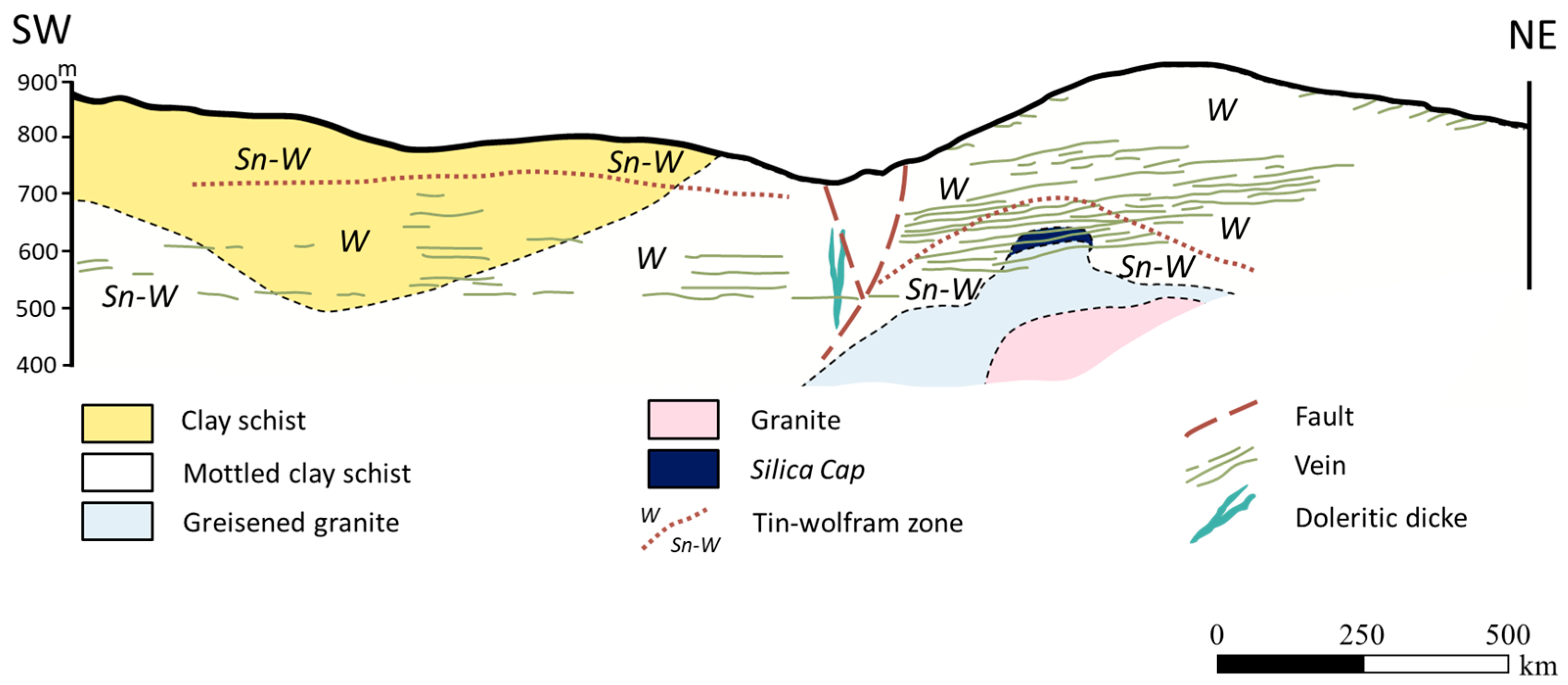
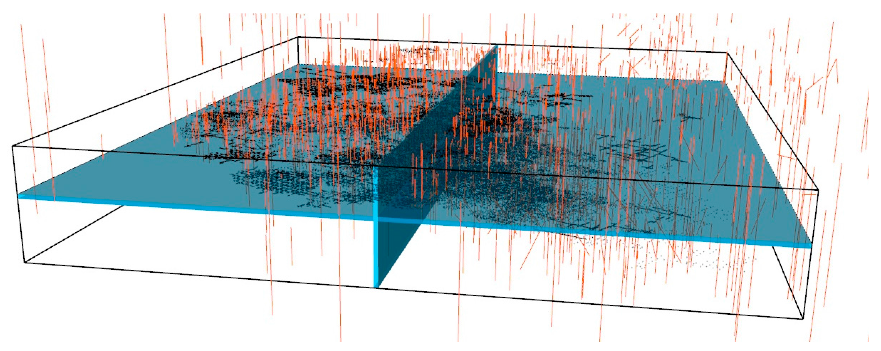
Figure 2.
3D view of boreholes and vertical section Px81 and horizontal section Pz75 used in the section images for displaying results.
Figure 2.
3D view of boreholes and vertical section Px81 and horizontal section Pz75 used in the section images for displaying results.

Figure 3.
The results of stope vein proportion estimation (OK): Px81 (left) and Pz75 (right).
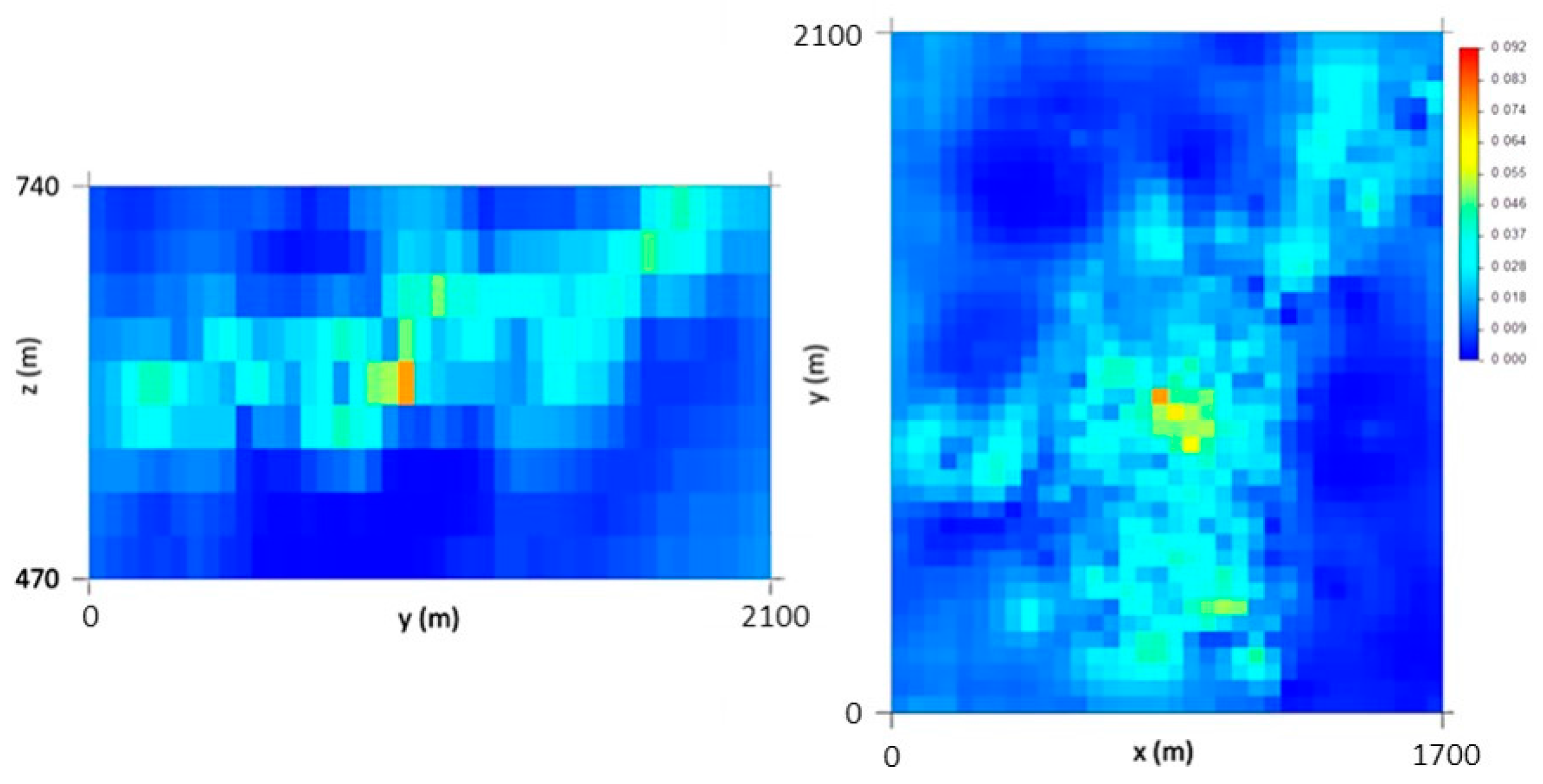
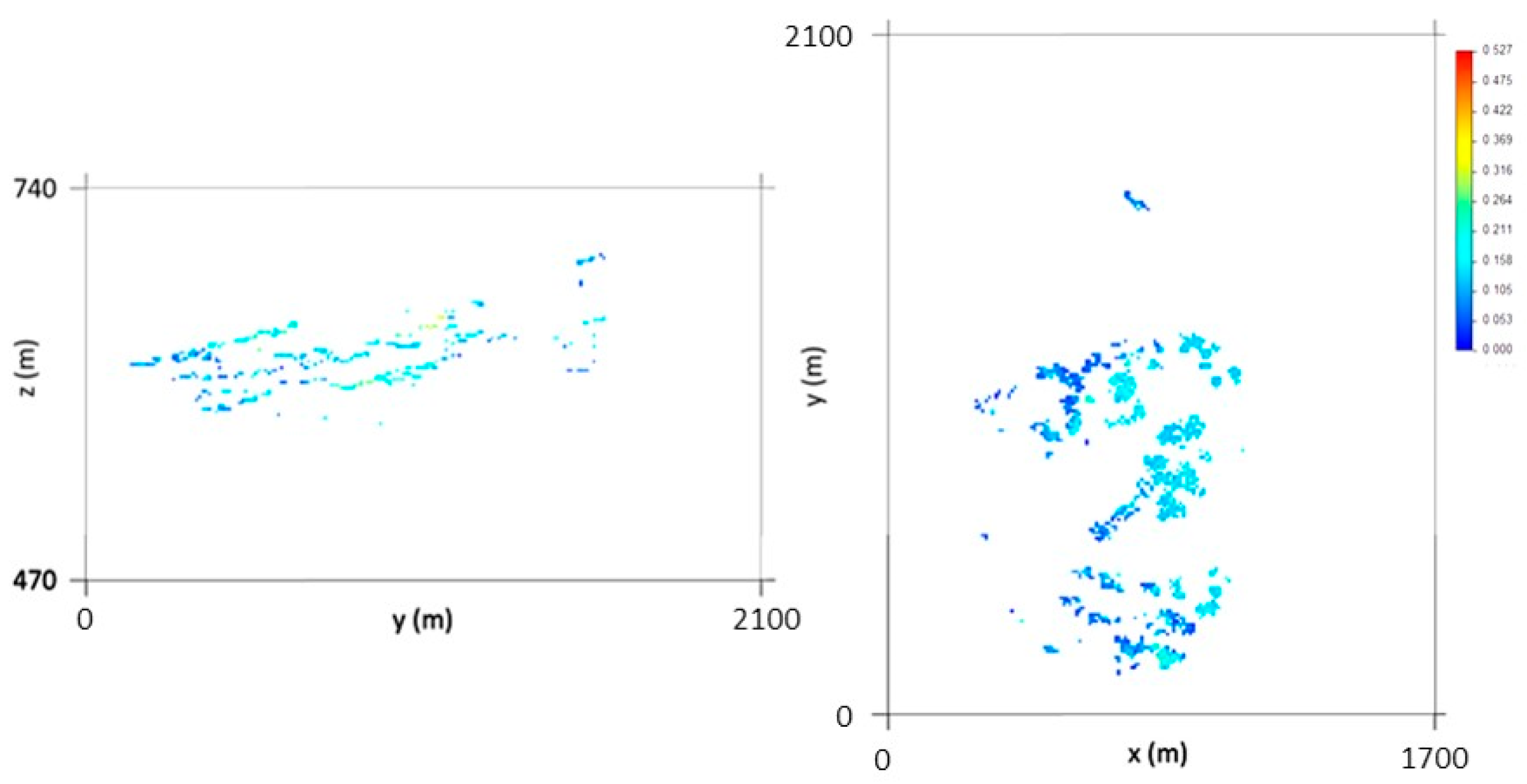
Figure 4.
Declustering results for stope vein proportion: Px81 (left) and Pz75 (right).

Figure 5.
Direct sequential simulation (DSS) first-phase results: Px81 (left) and Pz75 (right). The diagrams show one of 1000 scenarios.
Figure 5.
Direct sequential simulation (DSS) first-phase results: Px81 (left) and Pz75 (right). The diagrams show one of 1000 scenarios.

Figure 6.
Direct Sequential Simulation (DSS) first-phase results after correction of averages: Px81 (left) and Pz75 (right). The diagrams show one of 1000 scenarios.
Figure 6.
Direct Sequential Simulation (DSS) first-phase results after correction of averages: Px81 (left) and Pz75 (right). The diagrams show one of 1000 scenarios.

Figure 7.
DSS second-phase results: Px81 (left) and Pz75 (right). The diagrams show one of 1000 scenarios.
Figure 7.
DSS second-phase results: Px81 (left) and Pz75 (right). The diagrams show one of 1000 scenarios.
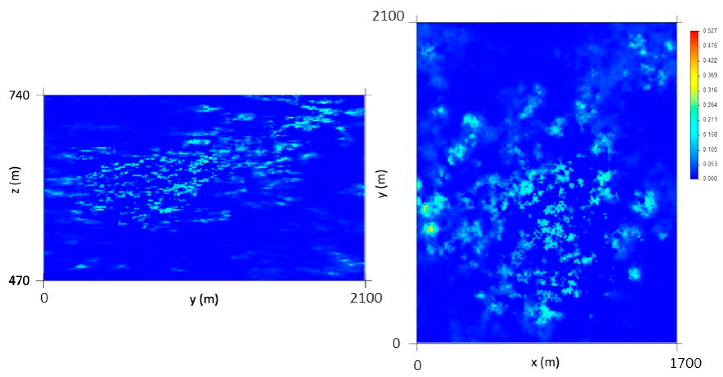
Figure 8.
Results of the final vein proportion model (average and coefficient of variation (CV)): Px81 (left) and Pz75 (right).
Figure 8.
Results of the final vein proportion model (average and coefficient of variation (CV)): Px81 (left) and Pz75 (right).
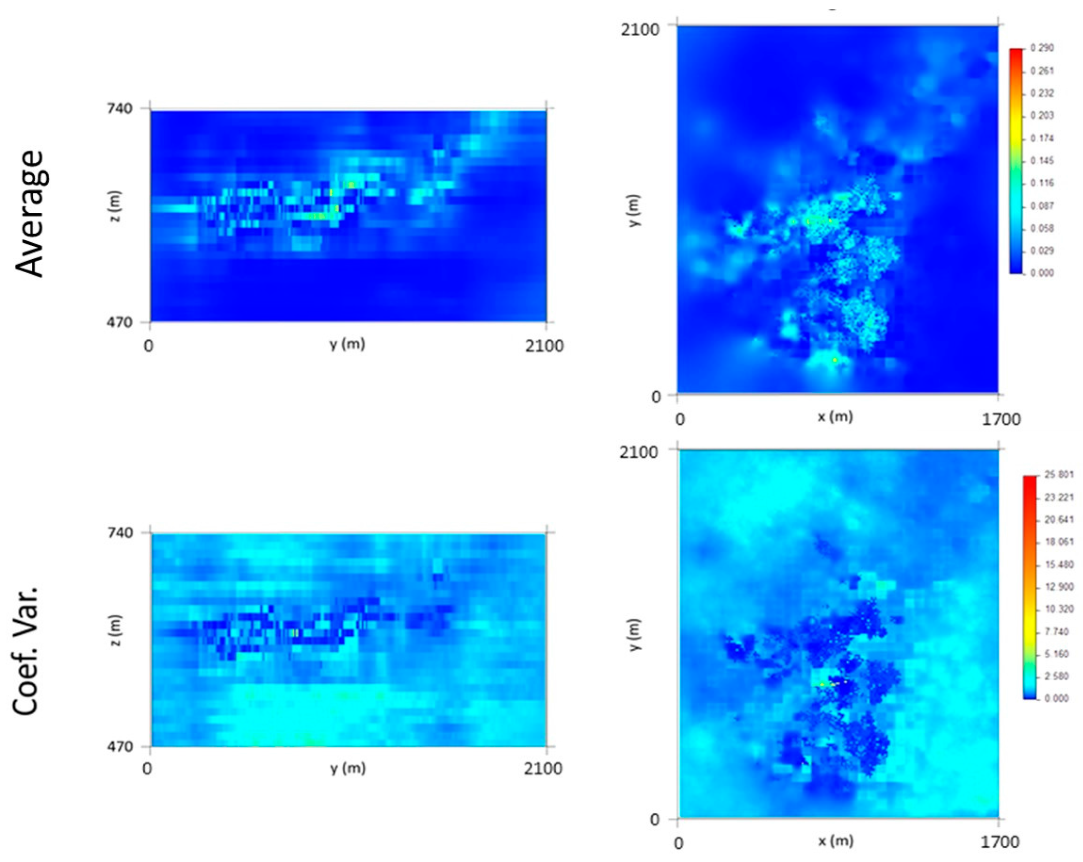
Figure 9.
Final model 3D representation: (a) vein proportion (>5% of vein); (b) Coefficient of variation (<10% uncertainty). Grid 10 m × 10 m × 10 m.
Figure 9.
Final model 3D representation: (a) vein proportion (>5% of vein); (b) Coefficient of variation (<10% uncertainty). Grid 10 m × 10 m × 10 m.

Figure 10.
Conditional cumulative histograms for L0: (a) for each class and (b) for grouped classes.
Figure 10.
Conditional cumulative histograms for L0: (a) for each class and (b) for grouped classes.
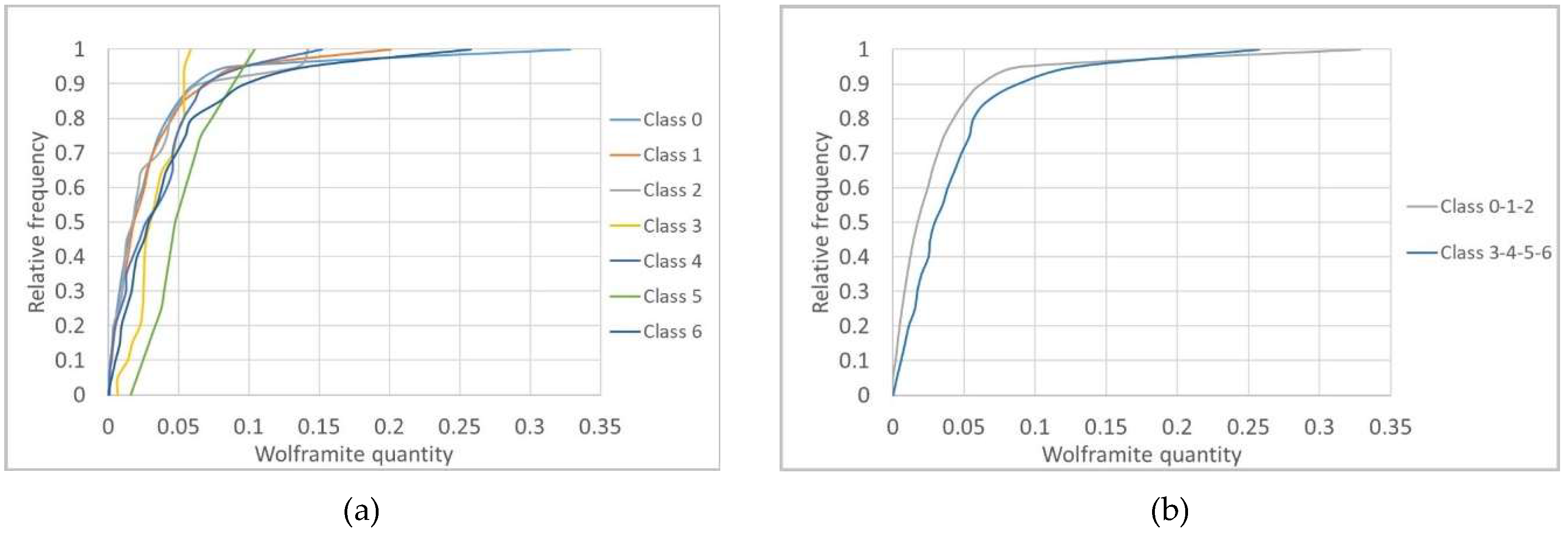
Figure 11.
Indicator Kriging results for the CL1 and CL2 class groupings: Px81 (left) and Pz75 (right).
Figure 11.
Indicator Kriging results for the CL1 and CL2 class groupings: Px81 (left) and Pz75 (right).

Figure 12.
Direct Sequential Simulation results for CL1 and CL2: Px81 (left) and Pz75 (right). The diagrams show 1 of 200 scenarios.
Figure 12.
Direct Sequential Simulation results for CL1 and CL2: Px81 (left) and Pz75 (right). The diagrams show 1 of 200 scenarios.
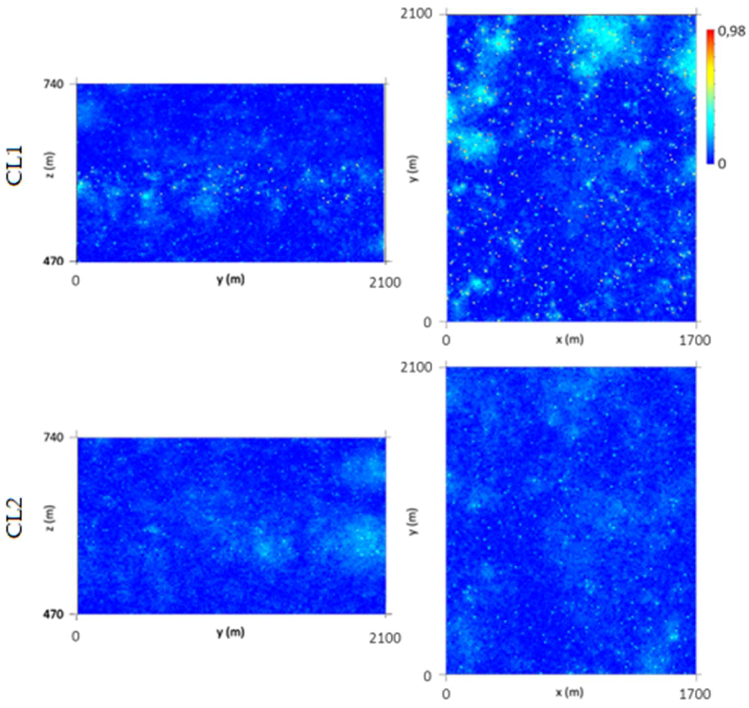
Figure 13.
Step 4 Monte Carlo procedure for building composite histograms: (a) CL1 cumulative histogram; (b) CL2 cumulative histogram; and (c) composite cumulative histogram (Prob {CL1} = 0.9159 and Prob {CL2} = 0.0841).
Figure 13.
Step 4 Monte Carlo procedure for building composite histograms: (a) CL1 cumulative histogram; (b) CL2 cumulative histogram; and (c) composite cumulative histogram (Prob {CL1} = 0.9159 and Prob {CL2} = 0.0841).


Figure 14.
Probability Field Simulation (PFS) procedure: Gaussian Sequential Simulation (GSS) U [0, 1] transformation; and PFS simulation. The diagrams show 1 of 1000 scenarios.
Figure 14.
Probability Field Simulation (PFS) procedure: Gaussian Sequential Simulation (GSS) U [0, 1] transformation; and PFS simulation. The diagrams show 1 of 1000 scenarios.

Figure 15.
Results for the final model of wolframite quantity (in kg/m3) (average and coefficient of variation): Px81 (left) and Pz75 (right).
Figure 15.
Results for the final model of wolframite quantity (in kg/m3) (average and coefficient of variation): Px81 (left) and Pz75 (right).

Figure 16.
Results for the model of final mineral potential (in kg) (average and coefficient of variation): Px81 (left) and Pz75 (right).
Figure 16.
Results for the model of final mineral potential (in kg) (average and coefficient of variation): Px81 (left) and Pz75 (right).
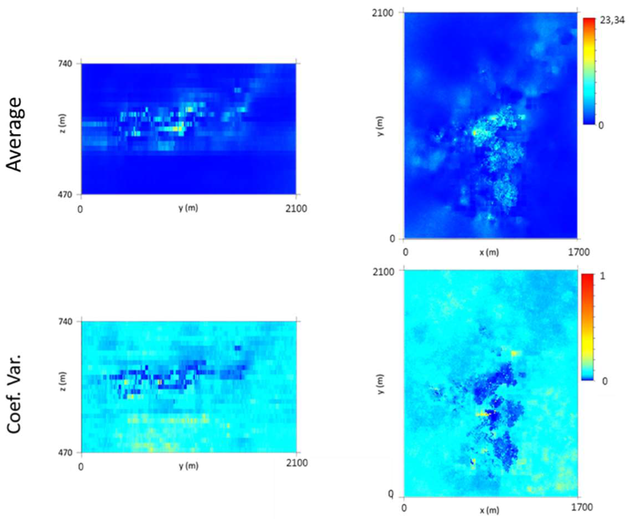
Figure 17.
Mineral potential curves: (a) Cumulative wolframite quantity (tons) as a function of vein proportion; (b) cumulative wolframite quantity (tons) as a function of elevation.
Figure 17.
Mineral potential curves: (a) Cumulative wolframite quantity (tons) as a function of vein proportion; (b) cumulative wolframite quantity (tons) as a function of elevation.

Figure 18.
3D view of the average wolframite potential in tons. The representation is made using the final grid resolution of 10 m × 10 m × 10 m.
Figure 18.
3D view of the average wolframite potential in tons. The representation is made using the final grid resolution of 10 m × 10 m × 10 m.

Table 1.
Stope grid (10 m × 10 m × 2 m) settings.
| Axis | Lower-Left-Corner Coordinate (m) | Cell Size (m) | No Cells |
|---|---|---|---|
| OX | 0 | 10 | 170 |
| OY | 0 | 10 | 210 |
| OZ | 470 | 2 | 135 |
Table 2.
Borehole grid (50 m × 50 m × 30 m) settings.
| Axis | Lower-Left-Corner Coordinate (m) | Cell Size (m) | No Cells |
|---|---|---|---|
| OX | 0 | 50 | 34 |
| OY | 0 | 50 | 42 |
| OZ | 470 | 30 | 9 |
Table 3.
Final grid (10 m × 10 m × 10 m) settings.
| Axis | Lower-Left-Corner Coordinate (m) | Cell Size (m) | No Cells |
|---|---|---|---|
| OX | 0 | 10 | 170 |
| OY | 0 | 10 | 210 |
| OZ | 470 | 10 | 27 |
© 2017 by the authors. Licensee MDPI, Basel, Switzerland. This article is an open access article distributed under the terms and conditions of the Creative Commons Attribution (CC BY) license (http://creativecommons.org/licenses/by/4.0/).
Share and Cite
MDPI and ACS Style
Sanches, A.; Almeida, J.; Sá Caetano, P.; Vieira, R. A 3D Geological Model of a Vein Deposit Built by Aggregating Morphological and Mineral Grade Data. Minerals 2017, 7, 234. https://doi.org/10.3390/min7120234
AMA Style
Sanches A, Almeida J, Sá Caetano P, Vieira R. A 3D Geological Model of a Vein Deposit Built by Aggregating Morphological and Mineral Grade Data. Minerals. 2017; 7(12):234. https://doi.org/10.3390/min7120234
Chicago/Turabian StyleSanches, André, José Almeida, Paulo Sá Caetano, and Romeu Vieira. 2017. "A 3D Geological Model of a Vein Deposit Built by Aggregating Morphological and Mineral Grade Data" Minerals 7, no. 12: 234. https://doi.org/10.3390/min7120234
Note that from the first issue of 2016, this journal uses article numbers instead of page numbers. See further details here.