Geostatistical Methodology to Characterize Volcanogenic Massive and Stockwork Ore Deposits


NOVA University of Lisbon, Faculty of Sciences and Technology, Earth Sciences Department and GeoBioTec, Quinta da Torre, 2829-516 Caparica, Portugal
*
Author to whom correspondence should be addressed.
Minerals 2017, 7(12), 238; https://doi.org/10.3390/min7120238
Submission received: 27 October 2017
/
Revised: 20 November 2017
/
Accepted: 27 November 2017
/
Published: 30 November 2017
(This article belongs to the Special Issue Geological Modelling)
Abstract
:The Zambujal ore deposit, Neves-Corvo mine, is a zoned volcanogenic sulfide deposit of copper and zinc, with massive ores at the top and stockwork ores at the bottom. Metal grades are strongly zoned by ore types. The main methodology hereby proposed combines geostatistical techniques so that an improved stochastic geological model of the Zambujal deposit encompassing morphology and grades is presented. The model of the morphology was made in two main steps. First, a 3D solid of the boundaries was created and then a 3D grid model of the local sulfide proportion was simulated. This latter variable was modeled by using rock specific gravity as a proxy. After that, a conditional grid model of relative copper grades, i.e., recalculated metal grades assuming only the sulfide content, is also simulated in accordance with the morphology. At the end, the new tool, metal tonnage cut-off surface, is proposed, which combines copper grades within massive ores and stockwork ores. To validate the results found, the global tonnages of copper obtained by Ordinary Kriging and the proposed methodology are compared.
1. Introduction
Geological models and metal grade models are fundamental tools used in the mining industry [1]. Both models are generated and constantly updated by taking into account the geological and geochemical information, gathered during the investigations performed at different stages of a mining project. The information provided by the geological modeling helps to better understand the geological behavior of the study area, the spatial distribution of the ores and metal grades, and to further optimize the mining works and mine planning.
The use of geostatistics for modeling mineral deposits boomed with the vulgarization of drilling techniques, sampling and analytical determinations. Despite the increased computational sophistication, traditional geological mapping plays an important role in modern modeling, because it is a heuristic method of passing information to geological models [2,3].
Traditionally, the construction of a mineral deposit model involves the characterization of the morphology and the contents of the elements with economic interest and penalties. In general, the geostatistical evaluation of ore resources encompasses the main steps [1]: (i) definition of the objectives of the study and database inventory, (ii) subdivision of the volume of interest of the mineral deposit into a few regions according to contact with host rock, different ore types, etc. (morphological model), (iii) zoning analysis of the mining variables according to the regions, (iv) creation of a spatial model of each variable under study, (v) estimation of the values of each variable in the non-sampled locations supported by a regular grid of blocks (model of metal grades), (vi) validation of the estimated model, ensuring the consistency of the model with the available data and the geological domains, (vii) evaluation of resources and build of cut-off curves, and (viii) characterization of the local uncertainty by the simulation of multiple scenarios. The uncertainty balances the available information and its heterogeneity, and can further be used to plan newer boreholes [4].
A morphological model represents both the boundaries of the deposit and the ensemble of ore types, which conditions the metals contents. In simple shape ore deposits, such as the stratigraphical ones, modeling involves estimation of top and bottom surfaces. In more irregular shape deposits, such as those of massive sulfides, the contact with the host rock is diffused and irregular, so possible procedures are manual digitization of boundaries along several cross-sections, interpolation of surfaces, and building a 3D solid (explicit modelling) [4,5]. Implicit modelling, encompassing the selection of isovalues of scalar properties previously estimated over the entire volume of interest, emerges as an alternative procedure [6,7]. When several types of ores condition the metal contents or properties of interest, a high-resolution grid model of ore type is constructed. Here, geostatistical methodologies, based on truncated plurigaussian modeling [8,9], or indicator formalism [10,11], such as indicator kriging (IK), sequential indicator simulation (SIS), or simulation with multipoint statistics [4], are currently being used.
The model of grades is primordially used for metal resources evaluations and cut-off curves and should be built in accordance with the experimental data and the morphological model [1]. For this purpose, geostatistical estimation methodologies provide the best linear unbiased and minimum error solutions (kriging). On the other hand, geostatistical simulation methodologies provide several results with the same probability of occurrence, which can then together be treated for local uncertainty evaluation purposes (Turning Bands Method, Sequential Gaussian Simulation (SGS), and Direct Sequential Simulation (DSS)) [10,12,13,14,15].
The results of kriging give a global estimate of resources. The simulation allows the generation of several plausible scenarios with similar probability of occurrence, which reproduces the spatial variability of the phenomenon by imposing the cumulative distribution function (cdf) of the data, the variogram and the data in its location [16]. The ensemble of simulated images can be used to characterize the local and global uncertainty of the phenomenon under study, the planning of exploration sequences and economic feasibility studies [11]. The two approaches, estimation and simulation should be both applied in any case study, and globally they report similar quantities [17,18].
The Zambujal deposit of metal sulfides (Neves-Corvo Mine, Alentejo, Southern Portugal) is the challenge case study examined in this paper. Lundin Mining Corporation, who also supplied the data for the study, operates the deposit. The Zambujal deposit is a volcanogenic massive sulfide deposit (VMS) of copper and zinc located in the southern Portuguese sector of the Iberian Pyrite Belt (IPB) [19]. It encompasses two ore types: massive ores (RM) in the top part and stockwork ores (RS) (both stringer and impregnation types) in the bottom part. The stockworks contain sulfide metals and host rock in variable proportions; it is important to note here that the extremely copper-rich ores in this domain reflect zone refining and late enrichment by the remobilization processes. Clarke of copper (Cu) is about 55 ppm (0.0055%), and the concentration clarke in chalcopyrite is 34.5/0.0055 = 6270 [20]; in economic terms, the group of VMS constitutes of an important world supply of copper, which is one of the top five metals used today. A better understanding of the genesis of copper deposits, encompassing the spatial architecture of RM and RS ores is a critical issue concerning the extension of the already discovered deposits and the prospection for new ones.
The cut-off grade of the primary metal in sulfide deposits, encompassing massive and stockwork ores, should take into account the proportion of sulfides and host rock because flotation technologies are more efficient in stockwork ores than in massive ores [21]. For this reason, in this study, it was decided to model the morphological variable P(x), proportion of sulfides and host rock with geostatistical approaches by using the rock specific gravity (SG) as a proxy. Also, for metal grades, an auxiliary variable meaning relative Cu grades YCu(x) was modeled with geostatistics.
2. Materials and Methods
2.1. Geological Background
The Neves-Corvo mine is a world-class copper mine in Europe, with a mining area that covers 13.5 km2 and an exploration concession area of about 112 km2. The mine is located in the Alentejo region, about 220 km southeast of Lisbon. It exploits the richest ore deposit ever found in the IPB and contains more than 300 Mt of massive sulfides, which is now considered a giant volcanogenic massive sulfide [19,24,25,26,27]. Neves-Corvo encompasses six lenticular polymetallic orebodies, Neves, Corvo, Graça, Zambujal, Lombador, and Semblana, which lie on both flanks of a main anticline [28].
The abnormal geochemistry of the Neves-Corvo is unique compared to the other deposits in the IPB: it possesses uncommonly high copper to zinc ratios (100 Cu/(Cu + Zn) > 50%), which more than doubles the other known deposits. The massive sulfide orebodies usually exhibit a classic lateral and vertical metal zonation and rest on the felsic volcanic rocks. As a general rule, the copper-rich ores occur at the base of the massive sulfide lenses, sometimes overlain by zinc-rich ores. Understanding how exhalative volcanic massive sulfide deposits are formed, the environment in which they were formed, and how the metals are saturated during genesis are critical to the exploration and exploitation of these resources.
The Zambujal orebody, which is the focus of the present study, contains significant grades of copper and zinc. It is estimated to be aerially about 600 m by 550 m with a maximum thickness of 55 m [28]. As said, it encompasses a mixture of two ore types, predominant massive ores (RM) in the top part and stockwork ores (RS) (both stringer and impregnation types) in the bottom part.
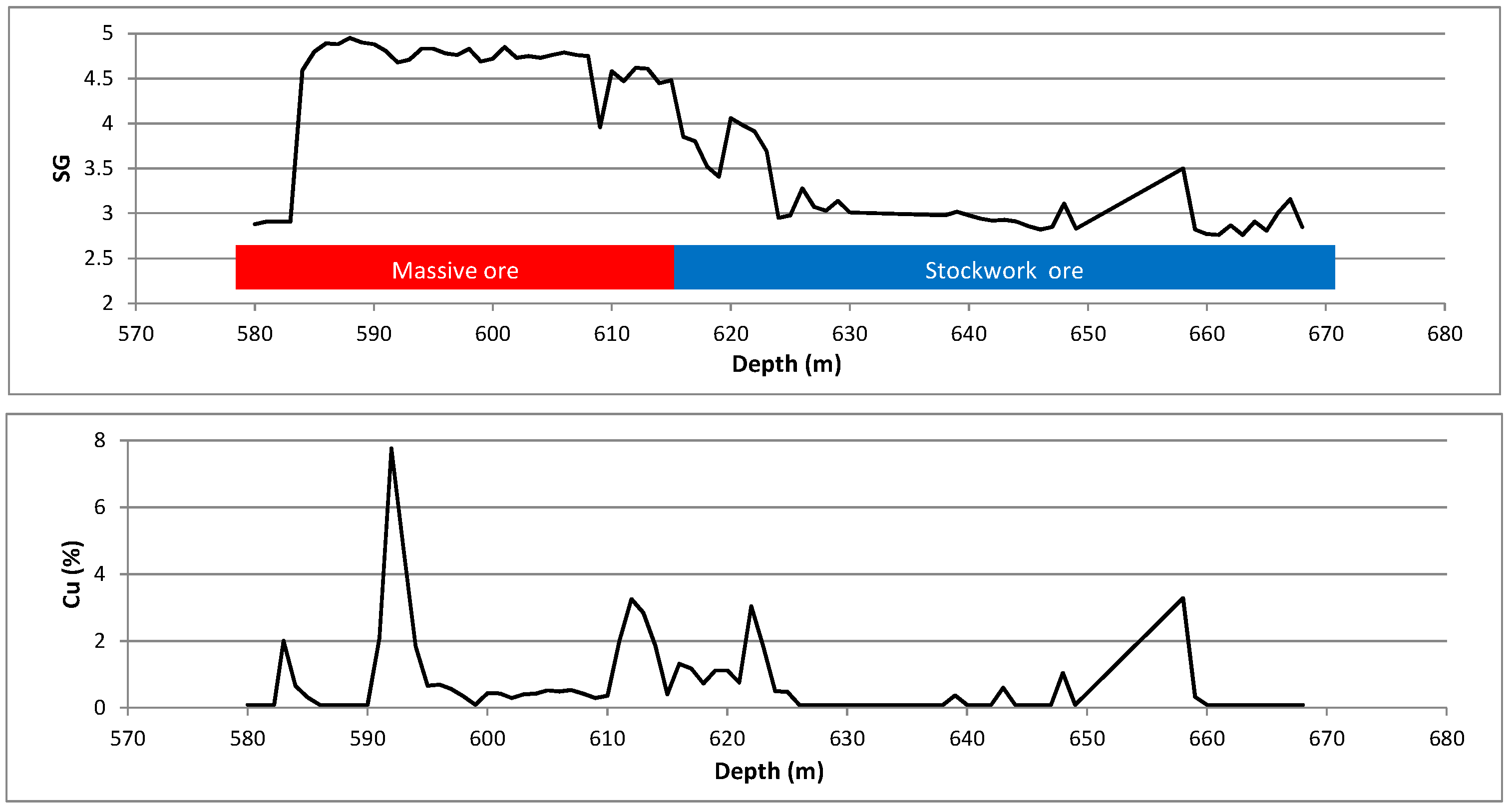
The massive sulfides mineralization always appears to be intercalated with the black shales, within locations with important silicified content. The massive lenses are connected and constitute single well-defined stratigraphic horizons in Neves-Corvo. The most predominant sulfur mineral is pyrite but chalcopyrite, sphalerite, and galena also occurs above 5%. Concerning the stockwork mineralization, stringer, or fissure ore, it is composed of anastomosing veinlets networks (feeder channels) and disseminations of sulfides that grade into massive sulfide lenses by coalescence of veins and replacements. Stockworks occur principally in highly silicified and chloritized footwall volcanic rocks. Sulfur minerals within stockwork ores are the same as within the massive ores, and host rock occurs in variable proportions. The transition between massive ores and stockwork ores is quick but without being abrupt, and this issue was decisive for the design of the methodology adopted in this study. Figure 1 above display the SG and Cu grades along the depth of one representative borehole intersecting the entire Zambujal orebody, the gradualness of the variations is clearly visible. Distinction between ore types is a prior classification made by the mine company.
2.2. Methodology
A data-driven methodology was designed taking into account the irregular shape of the Zambujal orebody, the blend between ores and the mining company recommendation for modeling a morphological random variable proportion of sulfides within the rock matrix P(x). Stockwork ores exhibit higher recovery of metals in mineral processing as compared to massive ores with equivalent grades, because flotation separation between chalcopyrite and pyrite is lower in efficiency than between chalcopyrite and host rock [21]. Despite the effective copper grades being much lower in the stockwork ores than in the massive ores (internal dilution due to blend of small veins with host rock), the copper grades in the fraction of sulfides within stockwork ores are in average more than the double of those in the massive sulfides, and this issue increases the relevance of the stockwork ores even in regions with poor copper grades.
Therefore, a high-resolution morphological model was built to quantify the local proportion of sulfides for each block of the grid model (the random variable P(x)), followed by a model of relative copper grades (the random variable YCu(x)) [29,30]. Both P(x) and YCu(x) are regionalized variables and can be modeled by using geostatistical tools [10,11], and the total amounts of metals and ores can be calculated directly from the estimated or simulated values of these variables.
For a sample location xi with a proportion of sulfide minerals P(xi) and effective grade of copper ZCu(xi), the relative grade of copper YCu(xi) is evaluated by (1).
For instance, if a sample had a grade of 2% copper and a P(x) = 0.7, then the relative grade of copper would be equal to 2%/0.7 = 2.86%. By doing so, the metal contents are recalculated and modeled for the sulfide fractions rather than modeling the total copper content.
Modeling of the variable P(x) is no doubt important however it is not measured at borehole cores. Thus, taking into account the principal paragenesis of the deposit, this work proposes the use of the lab-measured SG available for all core boreholes plus the grades of the chemical elements as proxy information for estimating P(x), first at borehole location and then for the entire deposit.
Combining grid models of both variables (P(x) and YCu(x)), a parametric resource of copper surface relating the cut-off grade of copper and the proportion of sulfides (morphological constraint) are readily constructed. The ability to construct such a surface in a straightforward way is an important objective and outcome of this work.
The proposed methodology encompasses the following main steps:
- Build a low-resolution 3D morphological model, delimiting the external boundaries and the main transition between massive ores in the top (RM) and stockwork ores in the bottom (RS). For the construction of this solid model, a classical procedure is used which involves digitalization of closed polygons in several almost parallel cross-sections, interpolation of surfaces, merger of surfaces in order to build a closed volume, and conversion of the volume into a voxel model (grid mining blocks).
- Taking into account the paragenesis of the Zambujal deposit, evaluate empirical cdf(s) of the random variable P(x) at boreholes locations conditional to the SG, grades of metals and sulfur grade all obtained from lab measurements to boreholes samples.
To compute local empirical cdf(s) of P(x), and as there is no linear relationship between P(x) and the set of measured variables, and solutions are not unique, we use an approach based on multivariate analysis. First, an extensive table combining all plausible mixtures of main minerals and host rock of the Zambujal paragenesis are made. According to XRD and microscope polished surface analysis already carried out by the mining company to several samples of ores [25], which are in line with the chemical analyzes, only four minerals are present in quantities above 5% that justify the classification proposed in this step: pyrite (FeS2, SG = 5.25), chalcopyrite (CuFeS2, SG = 4.20), sphalerite (ZnS, SG = 3.85) and galena (PbS, SG = 7.5) together with host rock (average SG = 2.70). For each mixture combination, theoretical values of SG’ and grades of Cu’, Zn’, Fe’, Pb’, and S’ are computed making use of the chemical formulas and the atomic weights of chemical elements.
For the sake of illustration; for a mixture of 30% of host rock with, 30% of pyrite and 40% of chalcopyrite, P(x) = 0.70, theoretical computed values are: Fe = 26.14%, S = 30.01%, Cu = 13.85%, and SG = 4.10. Another example, a mixture of 70% of host rock, with 8% of pyrite, 12% of chalcopyrite, 3% of sphalerite and 7% of galena, P(x) = 0.30, will have the following results: Fe = 7.38%, S = 10.39%, Cu = 4.16%, Zn = 2.01%, Pb = 6.06%, and SG = 3.52.
After this extensive theoretical table of mixtures is completed, each set of observed grades of Cu, Zn, Fe, Hg, and S and SG of each core sample of Zambujal are then compared with each row of the theoretical table, and the set of mixtures with the most similar grades and SG are selected. The set of selected rows are able to build a local empirical cdf of the variable P(x). To evaluate the similitude between theoretical values and lab-measured values, due to different variable dispersions, the Gower distance [31] is used.
- 3.
- For estimation plus simulation of ns1 scenarios of this variable, generate ns1 scenarios of P(x) for each borehole sample and compute their average. The Probability Field Simulation (PFS) algorithm [32] is used to draw values from the local cdf(s), instead of Monte Carlo simulation, as it accomplishes with both the local cdf(s) and the spatial continuity model of P(x).
- 4.
- Compute the auxiliary variable relative copper grade YCu(x) at sample locations. By using the values generated in step 3, ns1 scenarios of YCu(x) plus the average scenario are obtained.
- 5.
- Estimate regional cdf(s) of the studied random variables P(x), YCu(x) and SG(x) for both regions RM and RS by Indicator Kriging (IK) and estimate average images of those variables by Ordinary Kriging (OK) [33].
- 6.
- Build a high-resolution morphological model of P(x) only within the blocks of each region RM or RS, with Direct Sequential Simulation (DSS) conditional to the cdf(s) per ore type region [34].
- 7.
- Similarly to P(x), simulate the relative grade of Cu YCu(x) by using DSS conditional to cdf(s) per ore type region [34]; ns = ns1·ns2 realizations are simulated, ns2 for each one of ns1 realizations of P(x).
- 8.
For relative grades, where is the OK estimate of relative copper grade, the same values are given by
For simulated relative grades, the calculations are as follows:
For sake of validation, both results must be of the same magnitude: .
- 9.
- Evaluate uncertainty, computing local variance of the simulated values for P(x) and YCu(x).
- 10.
- Build a parametric global surface of copper metal tonnages and function of cut-off copper grades in massive ores and in stockwork ores.
Two notes:
- (1)
- Variables P(x), and are not stationary within the Zambujal deposit but are rather constrained to ore types. For this reason, it was essential to delimit RM and RS bodies with 3D computer solids and to constrain the simulations to the regional cdf(s) of the studied variables per RM or RS ore type. A modified version of DSS in which the simulated values are resampled from the regional cdf(s) is used to simulate the entire deposit [34] (steps 6 and 7 of the methodology).
- (2)
- The boreholes assays are made mostly at one meter length and the block size is 2 m × 2 m × 2 m (this is the size of the mining blocks used by the mining company, since it is considered the most suitable for stope design and mine planning). In order to make these scales compatible, prior to the application of the OK and DSS, the values of the boreholes are transferred to the blocks of the model that contained them, and when there are several samples in each block the arithmetic mean is made.
3. Case Study and Results
The case study follows the previous mentioned steps, combining geological heuristic mapping, kriging estimation and stochastic simulation algorithms. The database provided by Lundin Mining compiles information from more than 300 boreholes, for a total of about 58 km of drills. This database contains four tables of data concerning borehole information, survey, geology/ores and assays. With fewer exceptions, the boreholes assays are reported to one meter length intervals. It has implemented a quality assurance/quality control (QAQC) program to monitor sampling selection, sample preparation, and analytical process in order to assess the confidence in the stored data.
For sake of confidentiality, quantities are presented in all figures and tables previously multiplied by a constant.
3.1. Low Resolution 3D Morphological Model
The two mineralized domains RM and RS were manually digitized along several parallel cross-sections according to the borehole data and expertize heuristics. The distinction between RM and RS in boreholes used the classification already proposed by the mining company. Then, three surfaces were interpolated: the top of the massive ore (RM), the bottom of the massive ore/top of the stockwork ore (RS), and the bottom of the RS (Figure 2a). The digitalization ensures a closed volume between surfaces. Then, this model of surfaces was converted into a mining block model (block size 2 m × 2 m × 2 m, total number of blocks is 1,505,350) coded by RM or RS (Figure 2b).
3.2. Evaluate the Empirical Cdf of the Random Variable P(x) at Boreholes Locations
Before the geostatistical steps, the variable P(x) was estimated for all samples following the procedure mentioned in step 2 of Section 2.2. To make this estimate at the sample locations, the measured levels of the most abundant chemical elements (Fe, Cu, Zn, Sn, Pb, and S) were used, as well as the SG(x) of the sampled cores and the main minerals of the deposit (pyrite, chalcopyrite, galena, blend) plus host rock. Table 1 lists the main minerals of Zambujal, chemical formulas, specific gravity, and theoretical chemical element percentages according to the atomic numbers of the elements. It is important to emphasize the difference between the specific gravity of the host rock (about 2.8) and the specific gravity of the sulfide minerals (all above 4).
An extensive table listing all admissible combinations of these minerals and the host rock was then made with a resolution of 1% for proportion, and, for each combination, the theoretical values of the element grades (based on the chemical formulas) and the composite specific gravity were computed. Table 2 shows eight examples of the 4,598,126 identified as plausible.
Then, the laboratory-measured values of grades and SG are compared with each item of the extensive table, and a set of the closest combination of minerals plus host rock was extracted. Based on a sensitivity analysis for a selected set of 5% of the available assays [28], 10 theoretical mixtures of minerals plus host rock were considered sufficient to characterize the local empirical cdf. Each selected set of 10 values constitutes the local empirical cdf of P(x) variable at the locations of the boreholes. Figure 3a shows the histogram of the averages of the values of P(x) and Figure 3b shows the histogram of the coefficients of variation (dispersion measurement of the cdf).
Values of P(x) clearly show two populations, respectively, for RM and RS ores, and the separation threshold is about 0.6 (up to 60% of sulfides is stockwork, above 60% is massive ores). For the majority of the cdf(s), the coefficient of variance is low (for 80% of the cdf(s) it is below 0.15). The maximum observed range of P(x) (max-min) was 0.1 and the average range of all solutions was 0.04. These values substantiate the proposed estimation of the local P(x) cdf(s).
3.3. Estimation and Simulation of P(x), ZCu(x)and YCu(x) Variables
Cdf(s) of P(x) were used for variography, estimation and simulation of this variable within the entire deposit of Zambujal, as well as the calculation of relative grades YCu(x) at borehole locations.
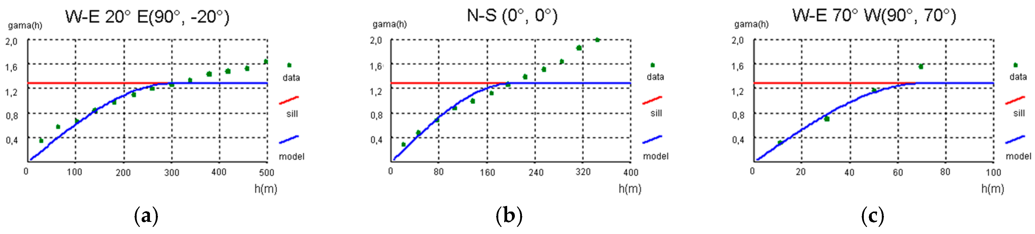
To identify the principal structural directions of the deposit, experimental variograms were computed for more than 20 directions according to the direction of the boreholes for all modeled variables [28]. Besides, for nugget effect evaluation, downhole variograms were also computed. Based on the results, three orthogonal directions: (1) W-E and 20° dip (90°; −20°), (2) N-S, horizontal (0; 0), and (3) W-E with 70° dip (90°; 70°) were selected as principal directions. The directions (1) and (3) are contained in the plane of the sections used in the previous step of digitalization, while the direction (3) intersects those sections. The nugget effect displayed by downhole variograms is about 5% for P(x) and 10% for ZCu(x) and YCu(x); because these amounts themselves are relatively low and with the upscaling between the borehole scale and the block model scale, no nugget effect was considered for OK or DSS.
Experimental variograms adjustments are of good quality for all variables. All variograms were fitted with spherical functions (SPH) and no nugget effect was added. Anisotropy ratio is remarkable for variables P(x) and SG(x) about 6×, major range is 300 m and minor range is 60 m. For grades and relative grades anisotropy ratio is much smaller about 1.33×, major range is about 40 m and minor range is 30 m. Figure 4 shows the experimental variograms for P(x) in the above-mentioned directions and Figure 5 the experimental variograms for YCu(x) for the same directions.
As explained before, the next experimental steps are: (i) draw values from the local cdf(s) of P(x), (ii) estimation of P(x), ZCu(x) and YCu(x) variables by OK, and (iii) DSS of P(x) and YCu(x) variables. Thirty realizations of P(x) plus three realizations of YCu(x) for each one of P(x) are performed: (ns = 90; ns1 = 30; ns2 = 3). Ninety realizations for YCu(x) are common for simulation of variables of this type, and the smooth appearance of the output images of uncertainty confirms this issue. Figure 5 shows a 3D view of a single from the thirty realizations of P(x) at the locations of the boreholes done by PFS. It became perceptible that the higher values are at the top of the structure and the lower values at the bottom.
The proportion of sulfide ore minerals P(x) was simulated using DSS for the two regions (RM and RS) at once. Instead of using a global cdf, the simulation of P(x) was performed using a modified version of DSS that uses local cdf(s) for each region, P(x)|RM and P(x)|RS. For declustering purposes, P(x)|RM and P(x)|RS are estimated using IK of 20 P(x) classes.
The simulation of relative copper grades YCu(x) follows the same approach as taken for P(x), namely the use of IK to estimate conditional cdf of YCu(x)|RM and YCu(x)|RS, followed by DSS with local histograms.
Figure 6 displays 3D views of average values of P(x) and YCu(x) variables. For sake of comparison, Figure 7 shows a set of results in an intermediate vertical cross-section of the model, W-E oriented.
From Figure 5, Figure 6a and Figure 7b,e,f, higher values of P(x) are located at the top of the structure, and lower values at the bottom, and the transition between the two regions is quick; in fact, histogram of Figure 3 supports this issue.
Figure 6b and Figure 7c,d,h,i show that the relative grades in stockwork ores are significantly higher than those in the massive ores. The transition of grades between regions is smooth, which is in accordance with the variability of the grades along the boreholes.
For sake of validation, histograms and variograms of selected realizations were computed and the results (Figure 8 show an example of one realization of P(x) and YCu(x)) show that they are quite well reproduced [28]. Also, copper grades were computed from the inverse relationship.
It is important to note that the values obtained with (5) are similar to the estimated ones, and the range is similar. This evidence is a good indicator that the proposed methodology can be applied and does not bias the results.
In addition, for validation of results, the average of grades obtained by using OK and DSS for the massive ore region, the stockwork ore region, and both regions combined is compared in Table 3. Deviations are very small, confirming that the use of relative grades YCu(x) and DSS with local histograms generates unbiased realizations.
3.4. Construction of the Tonnage-Surface Function for Copper Grades and Geological Dilution
Using the simulated values of the variables P(x) and YCu(x), average estimates for [P(xi)]*, [YCu(xi)]*, and [ZCu(xi)]* = [P(xi)]*·[YCu(xi)]* were computed for each mine block xi. The tonnage of copper (TCu) within each mine block xi with volume V and ore specific gravity SG(xi) is given by:
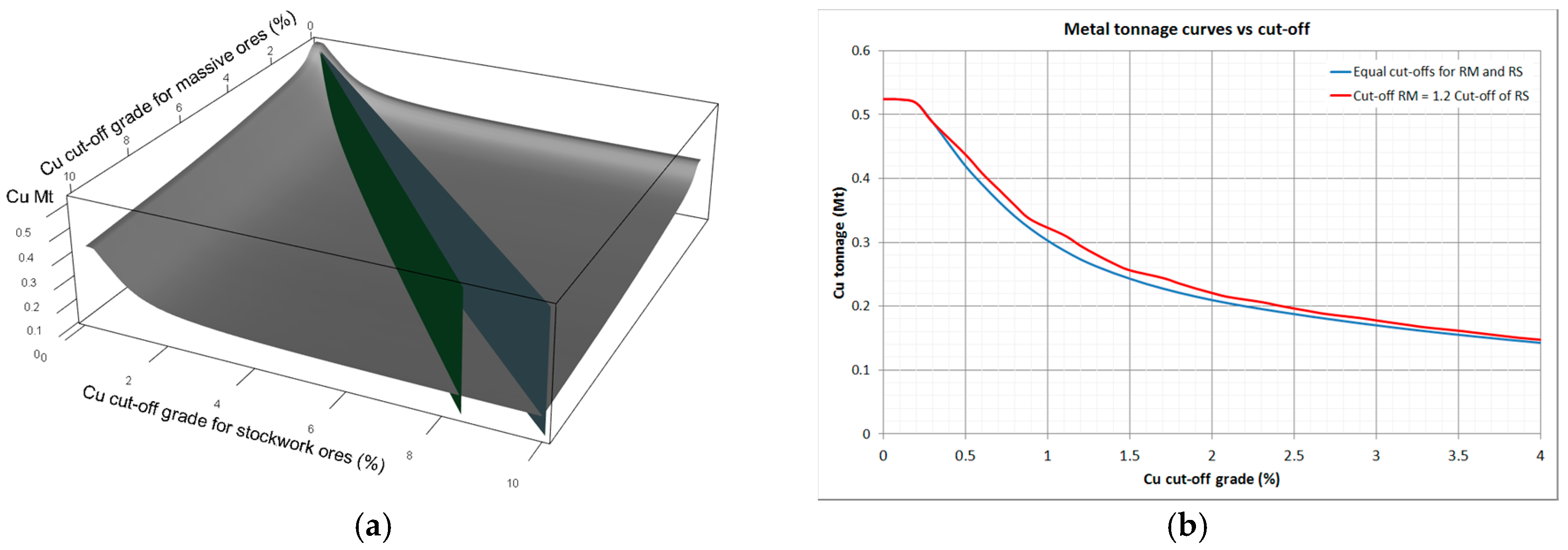
A surface representing the total average tonnage of copper as function of copper cut-offs for both massive (RM) and stockwork ores (RS) is now presented in Figure 9a; two vertical planes are also displayed: (blue) equal copper cut-offs for massive and stockwork ores; (green) cut-offs for massive ores are 1.2× of the ones of stockwork ores. The two corresponding cut-off curves, respectively for equal cut-off grades and richer copper cut-offs in RM than is RS (1.2×) are displayed in Figure 9b. The classification of each block as RM or RS ore type was done by applying a threshold value of 60% (0.6) to the morphological model of P(x) (see Figure 3a).
The maximum resource is 528,000 tons and is computed for all blocks independently of the copper grade and of being RM or RS ore type. If a Cu cut-off of 1.3% is applied for the entire deposit (RM + RS), the available copper tonnage is 261,905 tons (line in blue at Figure 9b). However, if a Cu cut-off of 1.3% is applied for the RM ore and Cu cut-off of 1.08% is applied for RS ores (line in red at Figure 8b, ), the available copper tonnage increased to 280,100 tons.
4. Discussion and Conclusions
The proposed methodology highlights the importance of the stockwork ores in the Zambujal deposit, and as mineral processing is more efficient in stockwork ores, metal cut-offs should take into account the proportion of sulfides relative to host rock. Also, Zambujal stockwork ores present lower grades of penalty elements, such as lead, arsenic, and bismuth.
When building a grade model of a VMS deposit with massive ores and stockwork, it is important to take into account the following issues:
- The proportion between sulfides and host rock P(x) can be modeled as a morphological random variable. Local values of P(x) at the borehole locations allow calculating the auxiliary variable relative copper grades YCu(x), meaning the hypothetical metal grades if host rock is not considered.
- Modeling the relative copper grades variable YCu(x) together with the proportion variable P(x), adds information to each mine block and enables the establishment of conditional cut-off grades to grades and morphology.
The variables in this study are modeled by using Ordinary Kriging (OK) and Direct Sequential Simulation (DSS). OK allows estimating the best unbiased total amount of ores and metal for each domain (RM and RS). In the present case study, OK and DSS results are of the same order of magnitude (see Table 3); hence, no bias was made in any calculation.
Given the available information, the realizations generated by the simulation algorithm, allows for an evaluation of the locations with highest uncertainty, taking into account the distance to the closest samples, the spatial continuity and the local heterogeneity of the observations. The Zambujal deposit has sufficient information to show results almost everywhere with confidence.
The proposed methodology is relevant in the sense that geostatistics demonstrated the importance of the stockwork ores in the Neves-Corvo deposits, in particular the Zambujal deposit. The Neves-Corvo deposit is known to possess an uncommonly high copper to zinc ratio. In the deeper parts of the ore masses, corresponding to the stockwork ores, it is important to note the extremely copper rich ores reflect zone refining and late enrichment. One relevant point is the fact that stockwork ores are usually undervalued because high metal grades are diluted by the host rock within this region.
Acknowledgments
The authors are grateful to the Lundin Mining Corporation for providing the data, information, and assistance required for the present work and to Midland Valley for providing an academic license for Move® software. This work is a contribution to Project UID/GEO/04035/2013 funded by FCT—Fundação para a Ciência e a Tecnologia in Portugal.
Author Contributions
David Silva and José Almeida conceived and designed the methodology and performed the experiments; David Silva wrote the paper.
Conflicts of Interest
The authors declare no conflict of interest. For sake of confidentiality, quantities presented in all figures and tables are multiplied by a constant.
References
- Rossi, M.E.; Deutsch, C.V. Mineral Resource Estimation; Springer: London, UK, 2014; p. 332. [Google Scholar]
- Almeida, J.A.; Soares, A.; Reynaud, R. Modelling the Shape of Several Marble Types in a Quarry. In Proceedings of the 24th International Symposium on Computer Applications in the Minerals Industries (APCOM), Montreal, QC, Canada, 31 October–2 November 1993; Elbrond, J., Tang, X., Eds.; Canadian Institute of Mining, Metallurgy and Petroleum: Montreal, QC, Canada, 1993; Volume 3, pp. 452–459. [Google Scholar]
- Castañón, C.; Arias, D.; Diego, I.; Martin-Izard, A.; Ruiz, Y. Resource and Reserve Calculation in Seam-Shaped Mineral Deposits; A New Approach: “The Pentahedral Method”. Minerals 2017, 7, 72. [Google Scholar] [CrossRef]
- Caers, J. Modeling Uncertainty in the Earth Sciences; Wiley-Blackwell, John Wiley & Sons Ltd.: London, UK, 2011. [Google Scholar]
- Mortensen, M.E. Geometric Modeling; John Wiley & Sons Inc.: New York, NY, USA, 1985. [Google Scholar]
- Cowan, E.J.; Beatson, R.K.; Ross, H.J.; Fright, W.R.; Mclennan, T.J.; Evans, T.R.; Carr, J.C.; Lane, R.G.; Bright, D.V.; Gillman, A.J.; et al. Practical implicit geological modelling. In Proceedings of the 5th International Mining Geology Conference, Bendigo, Australia, 17–19 November 2003; Dominy, S., Ed.; Australian Institute of Mining and Metalurgy: Carlton, Australia, 2003; pp. 89–99. [Google Scholar]
- Vollgger, S.A.; Crudena, A.R.; Ailleres, L.; Cowan, E.J. Regional dome evolution and its control on ore-grade distribution: Insights from 3D implicit modelling of the Navachab gold deposit, Namibia. Ore Geol. Rev. 2015, 69, 268–284. [Google Scholar] [CrossRef]
- Armstrong, M.; Galli, A.; Beucher, H.; Le-Loc’h, G.; Renard, D.; Doligez, B.; Eschard, R.; Geffroy, F. Plurigaussian Simulations in Geosciences; Springer: Berlin, Germany, 2011. [Google Scholar]
- Talebi, H.; Asghari, O.; Emery, X. Stochastic rock type modeling in a porphyry copper deposit and its application to copper grade evaluation. J. Geochem. Explor. 2015, 157, 162–168. [Google Scholar] [CrossRef]
- Goovaerts, P. Geostatistics for Natural Resources Evaluation; Oxford University Press: New York, NY, USA, 1997. [Google Scholar]
- Isaaks, E.H.; Srivastava, R.M. An Introduction to Applied Geostatistics; Oxford University Press: New York, NY, USA, 1989. [Google Scholar]
- Almeida, J.A. Stochastic simulation methods for characterization of lithoclasses in carbonate reservoirs. Earth-Sci. Rev. 2010, 101, 250–270. [Google Scholar] [CrossRef]
- Deutsch, C.V.; Journel, A.G. GSLIB: Geostatistical Software Library and User’s Guide; Oxford University Press: New York, NY, USA, 1998; p. 384. [Google Scholar]
- Almeida, J. Modelling of cement raw material compositional indices with direct sequential cosimulation. Eng. Geol. 2010, 114, 26–33. [Google Scholar] [CrossRef]
- Chiles, J.P.; Delfiner, P. Geostatistics: Modeling Spatial Uncertainty; Wiley: New York, NY, USA, 1999. [Google Scholar]
- Quental, P.; Almeida, J.A.; Simões, M. Construction of high-resolution stochastic geological models and optimal upscaling to a simplified layer-type hydrogeological model. Adv. Water Resour. 2012, 39, 18–32. [Google Scholar] [CrossRef]
- Charifo, G.; Almeida, J.A.; Ferreira, A. Managing borehole samples of unequal lengths to construct a high-resolution mining model of mineral grades zoned by geological units. J. Geochem. Explor. 2013, 132, 209–223. [Google Scholar] [CrossRef]
- Matias, F.; Almeida, J.; Chichorro, M. A multistep methodology for building a stochastic model of gold grades in the disseminated and complex deposit of Casas Novas in Alentejo, Southern Portugal. Resour. Geol. 2015, 65, 361–374. [Google Scholar] [CrossRef]
- Rosa, C.; McPhie, J.; Relvas, J.M.R.S.; Pereira, Z.; Oliveira, T.; Pacheco, N. Facies analyses and volcanic setting of the giant Neves Corvo massive sulfide deposit, Iberian Pyrite Belt, Portugal. Miner. Depos. 2008, 43, 449–466. [Google Scholar] [CrossRef]
- Jensen, M.L.; Bateman, A.M. Economic Mineral Deposits; John Wiley and Sons: New York, NY, USA, 1981; p. 593. [Google Scholar]
- Gerson, A.; Napier, T. Integrated Approaches for the Study of Real Mineral Flotation Systems. Minerals 2013, 3, 1–15. [Google Scholar] [CrossRef]
- Soares, A. Direct Sequential Simulation and Cosimulation. Math. Geosci. 2001, 33, 911–926. [Google Scholar]
- Nunes, R.; Almeida, J.A. Parallelization of sequential Gaussian, indicator and direct simulation algorithms. Comput. Geosci. 2010, 36, 1042–1052. [Google Scholar] [CrossRef]
- Tornos, F. Environment of formation and styles of volcanogenic massive sulfides: The Iberian Pyrite Belt. Ore Geol. Rev. 2006, 28, 259–307. [Google Scholar] [CrossRef]
- Gaspar, O.C. Paragenesis of the Neves-Corvo volcanogenic massive sulphides. Comunicações Serviços Geológicos Port. 1991, 77, 27–52. [Google Scholar]
- Barriga, F.J.; Carvalho, D.; Ribeiro, A. Introduction to the Iberian Pyrite Belt. In Geology and VMS Deposits of the Iberian Pyrite Belt; Neves Corvo Field Conference; Guidebook Series; Barriga, F.J., Carvalho, D., Eds.; Society of Economic Geologists: Lisbon, Portugal, 1997; Volume 27. [Google Scholar]
- Relvas, J.; Barriga, F.; Pinto, A.; Ferreira, A.; Pacheco, N.; Noiva, P.; Barriga, G.; Baptista, R.; Carvalho, D.; Oliveira, V.; et al. The Neves-Corvo Deposit, Iberian Pyrite Belt, Portugal: Impacts and Future 25 years after the Discovery. In Integrated Methods for Discovery: Global Exploration in 21st Century, Society of Economic Geologists Special Pub; Goldfarb, R., Nielsen, J., Eds.; Society of Economic Geologists: Littleton, CO, USA, 2002; Volume 9, pp. 155–176. [Google Scholar]
- Silva, D. Modelação Estocástica do Depósito Mineral do Zambujal (Mina de Neves-Corvo): Contribuição da Densidade como Indicador Morfológico. Master’s Thesis, FCT—Nova University of Lisbon, Monte da Caparica, Portugal, 2015. (In Portuguese). [Google Scholar]
- Almeida, J.A.; Soares, A.; Mariano, A.C.; Albuquerque, A. Zonal control of reserves estimation of a diamond alluvial deposit. In Proceedings of the Conference on Mining Geostatistics, Berg-en-dal, Kruger National Park, South Africa, 19–22 September 1994; Geostatistical Association South Africa: Berg-en-dal, Kruger National Park, South Africa, 1994; pp. 159–167. [Google Scholar]
- Almeida, J.A.; Soares, A.; Albuquerque, A. Zonal control to estimate classes of histograms: Application to a diamond alluvial deposit. In Geostatistics Wollongong ’96; Baafi, E.Y., Schofield, N.A., Eds.; Kluwer Academic Publishers: Dordrecht, The Netherlands, 1996; pp. 658–668. [Google Scholar]
- Gower, J.C. A general coefficient of similarity and some of its properties. Biometrics 1971, 27, 857–871. [Google Scholar] [CrossRef]
- Froidevaux, R. Probability field simulation. In Geostatistics Troia 1992; Soares, A., Ed.; Kluwer Academic Publishers: Dordrecht, The Netherlands, 1993; pp. 73–84. [Google Scholar]
- Soares, A.; Tavora, J.; Pinheiro, L.; Freitas, C.; Almeida, J. Predicting Probability Maps of Air Pollution Concentration: A Case Study on Barreiro/Seixal Industrial Area. In Geostatistics Troia 1992; Soares, A., Ed.; Kluwer Academic Publishers: Dordrecht, The Netherlands, 1993; pp. 625–636. [Google Scholar]
- Roxo, S.; Almeida, J.A.; Matias, F.V.; Mata-Lima, H.; Barbosa, S. The use of sensory perception indicators for improving the characterization and modelling of total petroleum hydrocarbon (TPH) grade in soils. Environ. Monit. Assess. 2016, 188, 1–19. [Google Scholar] [CrossRef] [PubMed]
- Gerst, M.D. Revisiting the cumulative grade-tonnage relationship for major copper ore types. Econ. Geol. 2008, 103, 615–628. [Google Scholar] [CrossRef]
Figure 1.
Specific gravity (SG) and Cu grades along the depth of one borehole intersecting the entire Zambujal deposit.
Figure 1.
Specific gravity (SG) and Cu grades along the depth of one borehole intersecting the entire Zambujal deposit.

Figure 2.
(a) 3D view of the three surfaces separating the two mineralized domains RM (massive ores) and RS (stockwork ores), top of RM in red, top of RS/bottom of RM in yellow and bottom of RS in blue; (b) grid block representation of the binary morphological two-regions RM (red) and RS (blue).
Figure 2.
(a) 3D view of the three surfaces separating the two mineralized domains RM (massive ores) and RS (stockwork ores), top of RM in red, top of RS/bottom of RM in yellow and bottom of RS in blue; (b) grid block representation of the binary morphological two-regions RM (red) and RS (blue).
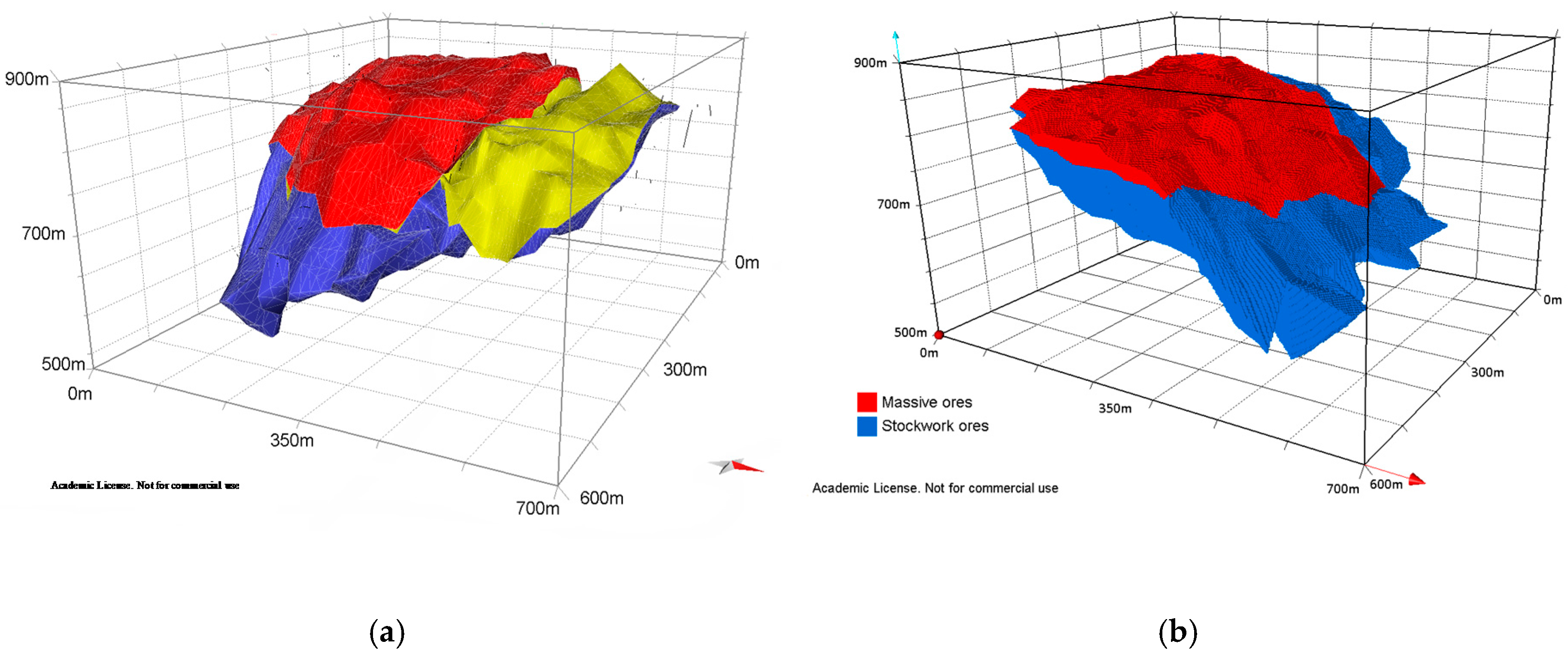
Figure 3.
(a) Histogram of average values of P(x) and (b) histogram of variation coefficients of P(x).
Figure 3.
(a) Histogram of average values of P(x) and (b) histogram of variation coefficients of P(x).
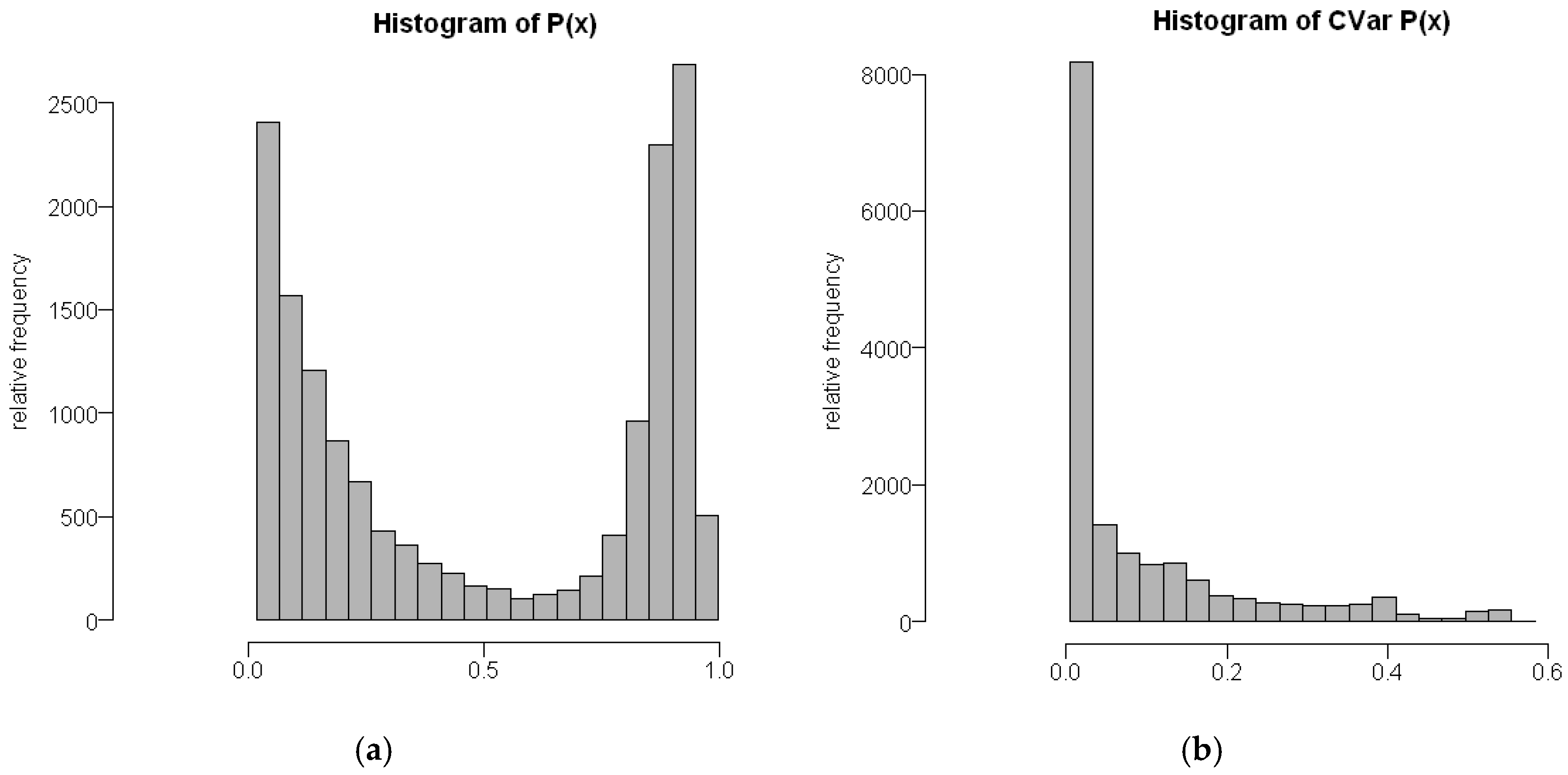
Figure 4.
Experimental variograms of P(x) and YCu(x) variables for the three mentioned directions: W-E 20° E (90°; −20°), N-S (0°; 0°) and W-E 70° W (90°; 70°). (a) SPH1 (C1 = 0.128; a1 = 300 m); (b) SPH1 (C1 = 0.128; a1 = 200 m); (c) SPH1 (C1 = 0.128; a1 = 60 m); (d) SPH1 (C1 = 15,127; a1 = 40 m); (e) SPH1 (C1 = 15,127; a1 = 30 m); (f) SPH1 (C1 = 15,127; a1 = 35 m).

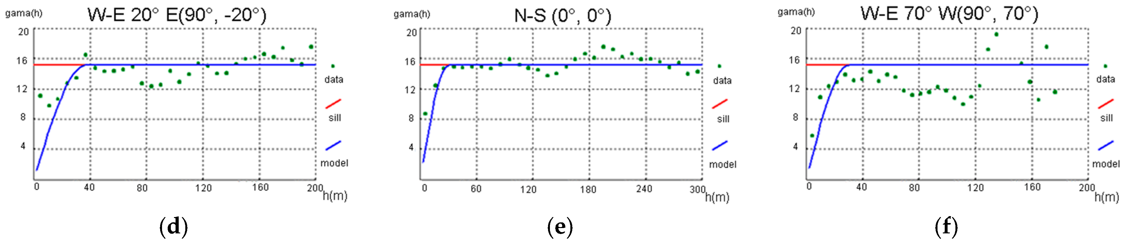
Figure 5.
3D view of a realization of P(x) at the locations of the boreholes. Red colors represent higher values of P(x) (massive ores at top), and blue-based colors refer to lower values of P(x) (stockwork ores at bottom).
Figure 5.
3D view of a realization of P(x) at the locations of the boreholes. Red colors represent higher values of P(x) (massive ores at top), and blue-based colors refer to lower values of P(x) (stockwork ores at bottom).
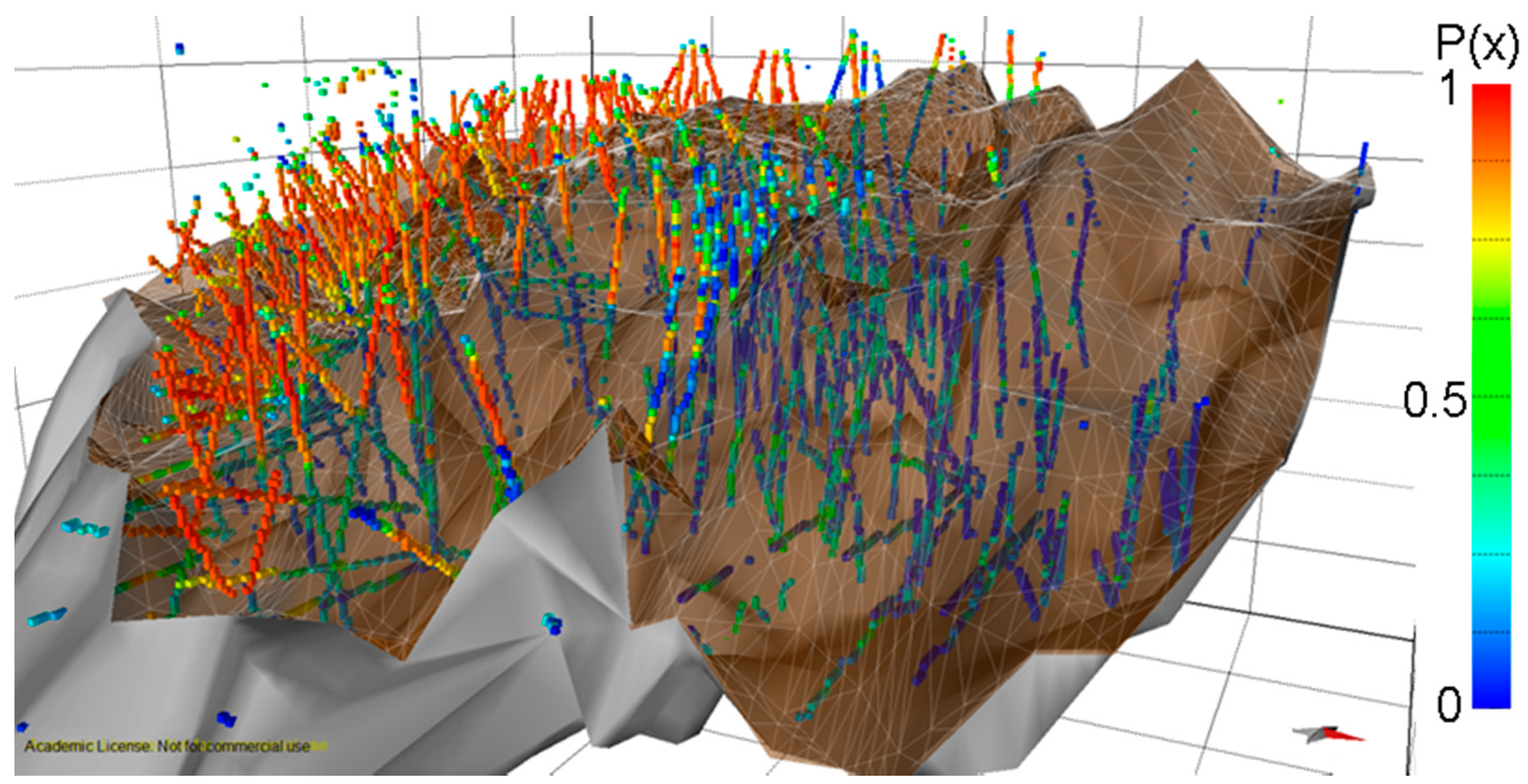
Figure 6.
3D view of (a) average values of proportion variable P(x); (b) average relative copper grades YCu(x) (%).
Figure 6.
3D view of (a) average values of proportion variable P(x); (b) average relative copper grades YCu(x) (%).
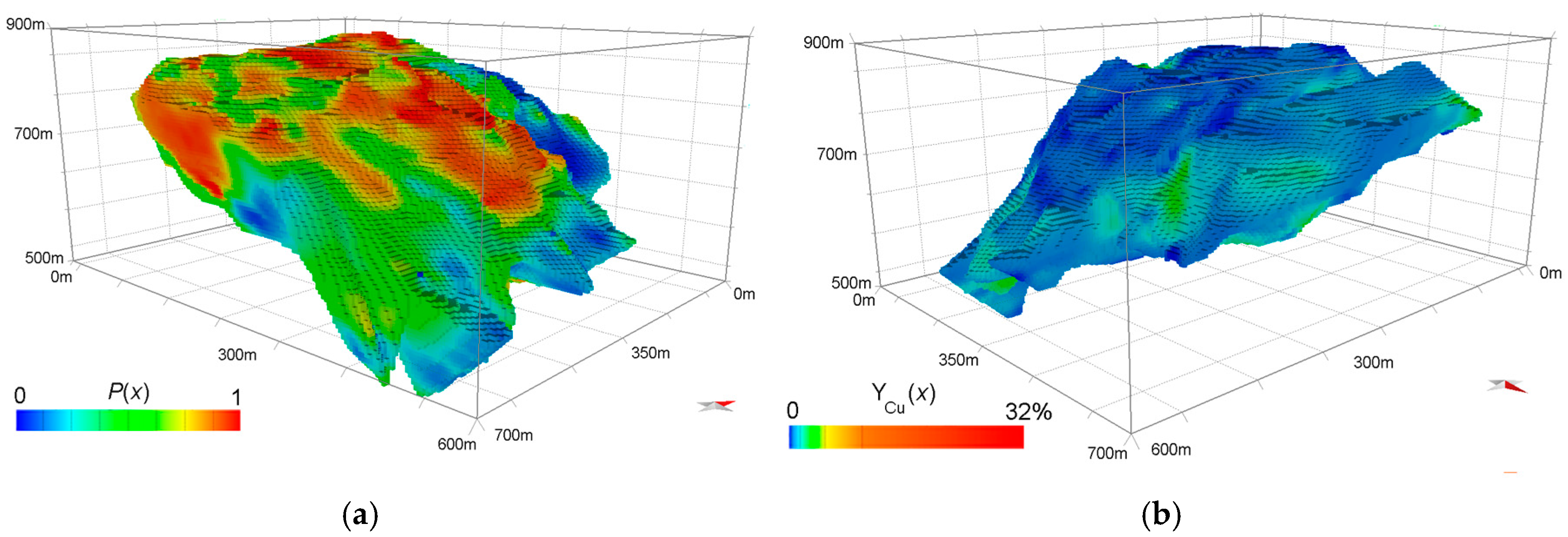
Figure 7.
Results in an intermediate cross-section: (a) RM (in blue) and RS (in red) regions according the 3D solid model; (b) kriging estimated image of P(x); (c) kriging estimated image of ZCu(x); (d) kriging estimated image of YCu(x); (e) one of the thirty simulated images of P(x); (f) average image of P(x) calculated from simulations; (g) image of variance (uncertainty) calculated from the set of simulated images of P(x); (h) one of the ninety simulated images of YCu(x); (i) average image of YCu(x) calculated from simulations; (j) image of variance (uncertainty) calculated from the set of simulated images of YCu(x); (k) binary image of variance (uncertainty) identifying the 25% of blocks with lower local variance calculated from the set of simulated images of P(x); (l) binary image of variance (uncertainty) identifying the 25% of blocks with lower local variance calculated from the set of simulated images of YCu(x).
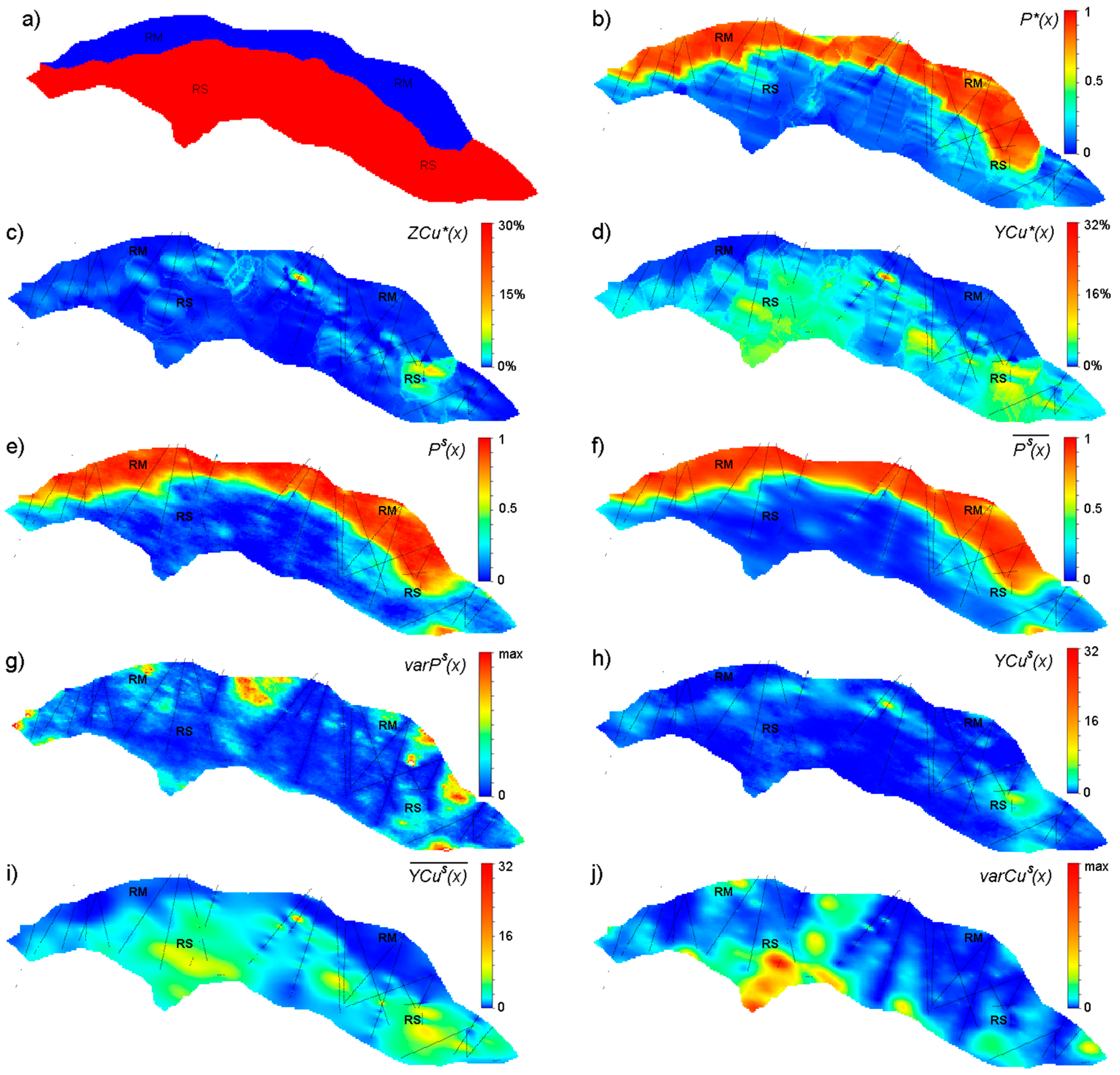
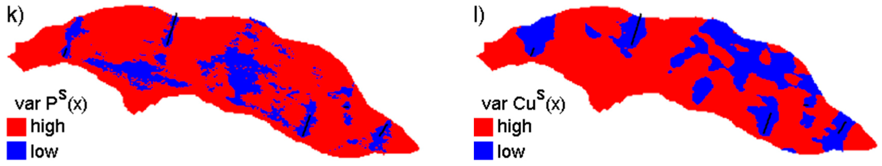
Figure 8.
Experimental variograms of P(x) and YCu(x) variables for the three OX, OY, and OZ directions: OX similar to W-E 20° E (90°; −20°), OY similar to N-S (0°; 0°) and OZ similar to W-E 70° W (90°; 70°). (a) SPH1 (C1 = 0.106; a1 = 300 m); (b) SPH1 (C1 = 0.106; a1 = 200 m); (c) SPH1 (C1 = 0.106; a1 = 60 m); (d) SPH1 (C1 = 14,986; a1 = 55 m); (e) SPH1 (C1 = 14,986; a1 = 30 m); (f) SPH1 (C1 = 14,986; a1 = 35 m).
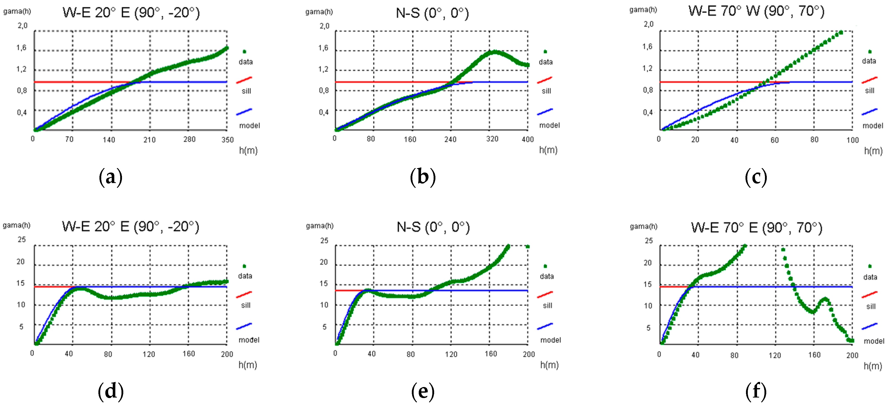
Figure 9.
(a) Copper tonnages resources as a function of copper cut-off grades for both massive ores (RM) and stockwork ores (RS); (b) cut-off curves corresponding to equal cut-off grades within RS and RS ores and richer copper cut-offs in RM than is RS (1.2×).
Figure 9.
(a) Copper tonnages resources as a function of copper cut-off grades for both massive ores (RM) and stockwork ores (RS); (b) cut-off curves corresponding to equal cut-off grades within RS and RS ores and richer copper cut-offs in RM than is RS (1.2×).


Table 1.
Main minerals of Zambujal, chemical formulas, specific gravity, and theoretical metal grades.
Table 1.
Main minerals of Zambujal, chemical formulas, specific gravity, and theoretical metal grades.
| Minerals/Rock | Formulas | SG | Fe (%) | S (%) | Cu (%) | Zn (%) | Pb (%) |
|---|---|---|---|---|---|---|---|
| Pyrite | FeS2 | 5.02 | 47 | 53 | |||
| Chalcopyrite | CuFeS2 | 4.20 | 30 | 35 | 35 | ||
| Sphalerite | ZnS | 4.00 | 33 | 67 | |||
| Galena | PbS | 7.50 | 13 | 87 | |||
| Host rock | 2.80 |
Table 2.
Eight examples of mixtures of sulfide minerals and host rock and calculated grades of Cu, Pb, Zn, S, and Fe and SG and P(x).
Table 2.
Eight examples of mixtures of sulfide minerals and host rock and calculated grades of Cu, Pb, Zn, S, and Fe and SG and P(x).
| Mixtures of Host Rock (HR) and Minerals (%) | Calculated Values of Grades (%) | SG’ | P’(x) | ||||||||
|---|---|---|---|---|---|---|---|---|---|---|---|
| HR | FeS2 | CuFeS2 | ZnS | PbS | Cu’ | Pb’ | Zn’ | S’ | Fe’ | ||
| 0 | 0 | 0 | 0 | 100 | 0 | 86.6 | 0 | 13.4 | 0 | 7.5 | 100 |
| 0 | 20 | 10 | 50 | 20 | 3.64 | 17.32 | 33.55 | 33.32 | 12.34 | 4.924 | 100 |
| 20 | 10 | 20 | 30 | 20 | 7.28 | 17.32 | 20.13 | 24.88 | 10.73 | 4.582 | 80 |
| 20 | 10 | 50 | 20 | 0 | 18.2 | 0 | 13.42 | 29.38 | 19.85 | 3.942 | 80 |
| 30 | 10 | 30 | 30 | 0 | 10.92 | 0 | 20.13 | 25.69 | 13.77 | 3.772 | 70 |
| 40 | 40 | 0 | 10 | 10 | 0 | 8.66 | 6.71 | 26.03 | 18.6 | 4.238 | 60 |
| 50 | 20 | 10 | 10 | 10 | 3.64 | 8.66 | 6.71 | 18.82 | 12.34 | 3.924 | 50 |
| 100 | 0 | 0 | 0 | 0 | 0 | 0 | 0 | 0 | 0 | 2.7 | 0 |
Table 3.
Summary of ore volumes and tonnages, average proportions, mean and variance (VAR) of grades and relative grades obtained by Ordinary Kriging (OK) and Direct Sequential Simulation (DSS) approaches.
Table 3.
Summary of ore volumes and tonnages, average proportions, mean and variance (VAR) of grades and relative grades obtained by Ordinary Kriging (OK) and Direct Sequential Simulation (DSS) approaches.
| Variable | Item | RM | RF | RM + RF |
|---|---|---|---|---|
| 3D solid model | Number of blocks | 737,049 | 1,802,404 | 2,539,453 |
| Ore volume (m3) | 5,896,392 | 14,419,232 | 20,315,624 | |
| [SG(x)]OK | 4.394 | 3.125 | 3.497 | |
| Ore tonnage (tons) | 25,908,746 | 45,060,100 | 70,968,846 | |
| Morphological model of P(x) | [P(x)]OK | 0.756 | 0.184 | 0.350 |
| VAR[P(x)]OK | 1.18 × 10⁻⁶ | 1.42 | 0.097 | |
| [P(x)]DSS | 0.768 | 0.176 | 0.348 | |
| VAR[P(x)]DSS | 1.08 × 10⁻⁶ | 2.05 × 10⁻⁷ | 0.099 | |
| Copper metal grades ZCu(x) and copper relative grades YCu(x) | [ZCu(x)]OK | 1.050 | 0.549 | 0.695 |
| VAR[ZCu(x)]OK | 2.44 × 10⁻⁶ | 3.71 × 10⁻⁷ | 1.740 | |
| [YCu(x)]OK | 1.465 | 3.289 | 2,763 | |
| [YCu(x)]DSS | 1.482 | 3.339 | 2.795 | |
| [YCu(x)]OK·[P(x)] OK | 1.051 | 0.545 | 0.692 | |
| VAR[YCu(x)]OK·[P(x)] OK | 1.92 × 10⁻⁶ | 3.25 × 10⁻⁷ | 1.629 |
© 2017 by the authors. Licensee MDPI, Basel, Switzerland. This article is an open access article distributed under the terms and conditions of the Creative Commons Attribution (CC BY) license (http://creativecommons.org/licenses/by/4.0/).
Share and Cite
MDPI and ACS Style
Silva, D.; Almeida, J. Geostatistical Methodology to Characterize Volcanogenic Massive and Stockwork Ore Deposits. Minerals 2017, 7, 238. https://doi.org/10.3390/min7120238
AMA Style
Silva D, Almeida J. Geostatistical Methodology to Characterize Volcanogenic Massive and Stockwork Ore Deposits. Minerals. 2017; 7(12):238. https://doi.org/10.3390/min7120238
Chicago/Turabian StyleSilva, David, and José Almeida. 2017. "Geostatistical Methodology to Characterize Volcanogenic Massive and Stockwork Ore Deposits" Minerals 7, no. 12: 238. https://doi.org/10.3390/min7120238
Note that from the first issue of 2016, this journal uses article numbers instead of page numbers. See further details here.