Authigenic Mg-Clay Minerals Formation in Lake Margin Deposits (the Cerro de los Batallones, Madrid Basin, Spain)


Departamento de Geología y Geoquímica, Facultad de Ciencias, Universidad Autónoma de Madrid, Campus de Cantoblanco, C/Francisco Tomás y Valiente, 7, Módulo 06, 28049 Madrid, Spain
*
Author to whom correspondence should be addressed.
Minerals 2018, 8(10), 418; https://doi.org/10.3390/min8100418
Submission received: 18 August 2018
/
Revised: 10 September 2018
/
Accepted: 17 September 2018
/
Published: 20 September 2018
(This article belongs to the Special Issue Authigenic Clay Minerals: Mineralogy, Geochemistry and Applications)
Abstract
:The Madrid Basin contains large and well developed deposits of Mg-clays of Miocene age. These were developed in an environment controlled by a lacustrine saline-alkaline environment with an arid or semi-arid climate, leading to large deposits of Mg-clays. This paper summarizes the study about the formation of Mg-clay minerals in the transition from mudflat lithofacies made-up of Mg-smectite to palustrine lithofacies where sepiolite is predominant. The samples collected in the field were characterized by XRD (X-Ray Diffaction) (bulk sample and clay fraction), examined using SEM (Scanning Electron Microscopy) and analyzed by XRF (X-Ray Fluorescence) and FTIR (Fourier Transform Infrared Spectroscopy). The results suggest that during the formation of these materials dissolution-precipitation, direct precipitation and recrystallization mechanisms intervened. The type of water present (runoff, lake and/or groundwater) is a key factor for the development of the different mineral phases. In the case of the study, the analyzed series goes from mudflat conditions with influence of runoff water to a palustrine environment. During this evolution, the influence of groundwater increases with time. This is reflected in the affinity between the samples analyzed and the presence of certain elements that could serve as indicators of changes between different media.
1. Introduction
Looking for sedimentary environments in which both neoformation and diagenetic processes of Mg-clays can take place, the palustrine-lacustrine environment is highlighted [1]. According to Cowardin et al. [2] palustrine environment is related to inland wetlands commonly dominated by the presence of trees, shrubs, and emergent vegetation, ranging from permanently saturated or flooded land (as in marshes, swamps, and lake shores) to land that is wet only seasonally. Water chemistry is normally fresh but may range to brackish and saline in semiarid and arid climates. Under these conditions, the palustrine environment seems to be especially complex and indeed very suitable for the study of mineralogical and chemical changes of uncommon clay minerals such as sepiolite. Indeed, according to Jones [3], the transformation of preexisting clays seems particularly encouraged where the proportion of sediment to water is high and where there is important solute contents, such as wetlands (lacustrine-palustrine environment).
The Miocene successions cropping out in the Madrid Basin yield a rather large variety of industrial minerals and rocks, most of them occurring in lacustrine sequences [4]. These sequences are especially relevant because they contain deposits of evaporites (sodium salts) and clays (ceramic clays and Mg-clays) of economic interest. Certainly, the occurrence of large deposits of magnesian clays, made up mostly of fibrous clay minerals (sepiolite and palygorskite), kerolite-stevensite mixed layers and Mg-rich smectites (saponite and stevensite), is one of the most remarkable features of the Neogene sediments in the Madrid Basin (Spain) (Figure 1a) (see [5,6,7], and references therein).
During most of the Neogene, the basin was occupied by lacustrine and palustrine systems fringed by alluvial fan and fluvial distributary facies forming a centripetal drainage system [8]. The Neogene succession of the Madrid Basin has been divided into three main Miocene stratigraphic units (Lower, Intermediate and Upper) overlain by a relatively thin and discontinuous Pliocene sedimentary sequence (Figure 1b). The Miocene continental formations are sub-horizontal and extend largely towards the east and south forming the uppermost part of the sedimentary sequence that infills the basin. The boundaries between stratigraphic units are marked by paleokarstic surfaces and/or minor angular disconformities [7,9,10].
The Mg-clay deposits are located in a transition zone between alluvial and marginal lacustrine deposits mostly within the Miocene Intermediate Unit (lower Aragonian–lower Vallesian; 19-10 Ma) which is about 200 m thick. These deposits occur in different lithofacies that are laterally equivalent, restricted to the northwest and especially south-southwest of the basin (Figure 1a). The lithofacies association bearing Mg-clays was named “Magnesian Unit” by Pozo and Casas [11].
The coexistence of sepiolite and Mg-smectite clays in single or separated layers is common in many Mg-clay deposits of the Madrid Basin [12]. The variety of Mg-clay phases and their sedimentological settings is related to different geochemical pathways where water hydrochemistry (runoff, groundwater or lake water) and the presence/absence of inherited Al-clay minerals plays an outstanding role [13].
Taking into account the complexity of processes in the continental realm, the abundance and variety of Mg-clay deposits in the Madrid Basin makes possible a detailed study of the genetic interrelationship among them and the environmental constraints. Especially outstanding is the genetic relationship between Mg-smectite and sepiolite. Studies of sepiolite occurrences and origin in continental deposits are well supported by abundant literature [14,15,16]. However, studies about its genetic relationship with other Mg-clays are relatively scarce although fibrous and non-fibrous Mg-clays have been commonly recognized in the same deposit, suggesting a genetic relationship.
The aim of this paper is the detailed study of the formation of Mg-clay minerals in the transition from mudflat lithofacies made-up of Mg-rich smectite to palustrine lithofacies where sepiolite is predominant. The Batallones sepiolite deposit (Figure 2a) (Madrid Basin, Spain) has been chosen because it shows clear evidence of the above-mentioned transitional materials [17].
2. Geological Setting and Sampling
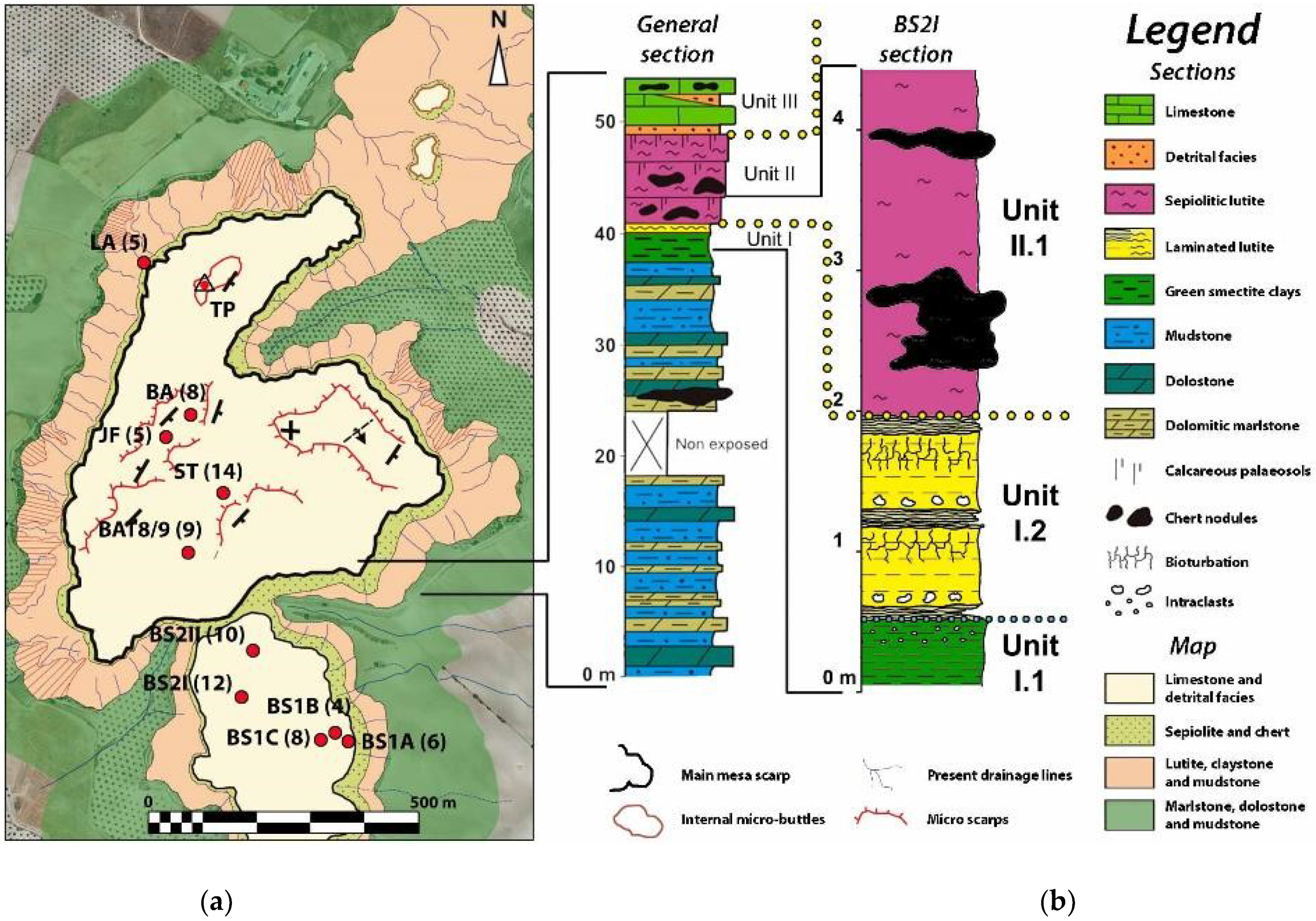
The Batallones sepiolite deposit is located at top of the Miocene Intermediate Unit of the Madrid Basin (Spain) (Figure 1b), between the villages of Torrejón de Velasco and Valdemoro (Province of Madrid). Three main lithological units have been distinguished in the sedimentary sequence from bottom to top (Figure 2b): (Unit-I) consists of mudstone, dolomitic marlstone and Mg-bentonite; (Unit-II) formed by sepiolite and opal-CT; and (Unit-III) made-up of limestone, marlstone and siliciclastic deposits [14,17,18].
The Mg-clay mineral occurrences are associated with Units I and II but the economic deposit of sepiolite is located in Unit II (Figure 2a). The top of Unit I comprises green to brown clays (I.1) passing upwards into massive and laminated to bedded mostly reddish lutites (I.2) (Figure 3). Two sub-units (II.1 and II.2) can be differentiated in the sepiolite deposit. Sub-unit II.1 is made up of sepiolite lutites showing massive and laminated textures. Subunit II.2 contains sepiolite-palygorskite dark lutites (yellowish gray to dark brown lutite) and calcretes that disconformably overlie subunit II.1. Lowermost clastic deposits of the overlying Unit III infill the irregularities of the paleo-relief surface (Figure 2b).
The mudstone and dolomite marl deposits of Unit I are interpreted as mudflat deposits formed in an alkaline-saline Mg-rich lake margin environment. Thick sepiolite and opal nodules from Unit II resulted from the development of polyphasic paleosols in a similar alkaline lake margin environment undergoing prolonged subaerial exposure alternating with discontinuous groundwater supply [17]. Siliceous beds and nodules included in the sedimentary sequence resulted from early diagenetic replacement of calcareous and/or lutite deposits, similar to other chert occurrences in the Madrid Basin [19,20].
Fifty-four samples from six lithological sections (ST, BS2II, BS2I, BS1C, BS1B, and BS1A) were collected. Their location and stratigraphic position are shown in Figure 2a and Figure 4. In addition, the mineralogical and geochemical composition of twenty-four samples from four lithological sections (LA, BA, JF, and BAT8/9) previously reported [17] were included for this study. The selected samples mostly belong to transitional Unit I.2. but there are also samples from the undelaying materials (I.1) and the base of the uppermost Unit II.1. The different lithofacies and units established in section BS2I (Figure 4) were considered representative for the remaining lithological sections.
3. Analytical Methodology
Mineralogical analysis of 54 samples (Table 1, Table 2 and Table 3) was carried out by means of X-ray diffraction (XRD) using a SIEMENS D-5000 equipment (Siemens AG, Gerätewerk-Karlsruhe, Germany) with a scanning speed of 1°2θ/min and Cu-Kα radiation (40 kV, 20 mA). XRD studies were carried out both on randomly oriented samples (bulk sample) and selected clay fraction samples (<2 μm). Powdered (<63 μm) whole-rock samples were scanned from 2° to 65° 2θ. Among the previously cited samples, 51 (Table 1, Table 2 and Table 3) were prepared from suspensions oriented on glass slides for identification of the clay fraction minerals was carried out on oriented air-dried samples, with ethylene glycol solvation, and after heating at 550 °C. The mineral intensity factors (MIF) method was applied to XRD peak intensity ratios normalized to 100% with calibration constants for the quantitative estimation of mineral contents [21,22,23]. This method is empirically determined to modify the reflection heights for differences due to the scattering power of different unit cells. The MIF constants provided for each mineral phase are referred to the unit intensity for a selected reference mineral (commonly corundum) as base for normalization. The method is cheap, straightforward and satisfactorily accurate. To establish the relative ordering (“crystallinity”) of sepiolite, the FWHM (Full Width at Half Maximum) parameter was measured on the (110) reflection at 1.2 nm in bulk sample [24]. The method proposed by Christidis and Koutsopoulou [25] was used for smectite type determination in five selected samples. To complete the study, the values of 25 samples previously reported by Pozo et al. [17] were also included.
Seventeen other selected samples were analyzed by standard petrography and 22 were examined under SEM (Philips SEM XL-30, Philips, Eindhoven, The Netherlands) after coating with gold (10 nm thick) in a sputtering chamber.
The chemical analysis of major (Si, Al, Fe, Ca, Ti, Mn, K, Mg, P, and Na) and trace elements (Ag, As, Ba, Be, Bi, Br, Cd, Ce, Co, Cr, Cs, Cu, Ga, Ge, Hf, I, La, Mo, Nb, Nd, Ni, Pb, Rb, Sb, Sc, Se, Sm, Sn, Sr, Ta, Th, Tl, U, V, W, Y, Zn, Zr, and Li) of 28 (Table A1) samples was performed by means of the MagiX X-ray fluorescence (XRF) spectrometer (PANalytical, Almedo, The Netherlands) of PANalytical. A Varian 220-FS QU-106, atomic absorption (AA) spectrophotometer (Varian, Inc., Victoria, Australia) was used for the determination of sodium. The chemical analysis values of 17 samples reported by Pozo et al. [17] were also included. For the normalization of geochemical data, the Upper Continental Crust values [26] were used.
The RMN analysis of 27Al in two samples was performed with a Bruker AV 400 WB spectrometer (Bruker, Wissembourg, France). The software package IBM SPSS Statistic 24 (IBM Corp., v.24, Armonk, NY, USA) was used to obtain the Pearson´s correlation coefficients and Cluster analysis (Ward method).
4. Results and Discussion
4.1. Mineralogical and Chemical Characterization
4.1.1. Unit I.1
This unit has a thickness of more than 8 m and consists of mostly green to yellowish massive mudstones containing minor proportions of silt and sand fractions, and occasionally soft clasts (lithofacies I.1-B). Inserted carbonate and marl beds (up-to 0.5 m thickness) are observed (lithofacies I.1-D). At the top, green to yellowish massive claystones displaying abundant slickensides and locally lamination and bioturbation commonly occur (lithofacies I.1.A) (Figure 5a). Occasionally, decimetric to metric sized calcite nodules is observed. Both at the top and inserted in I.1A, decimetric to metric thick beds of brown to yellow clay intraclast arenites are recognized (lithofacies I.1.C). This lithofacies is composed of a fine grained groundmass (matrix) and grain-supported sub-rounded lutite intraclasts.
The sedimentological interpretation is of mudflat deposits related to an alkaline-saline lake margin with Mg2+-rich waters [18].
Claystone (I.1-A)
The phyllosilicate content in this lithofacies is very high (>97%) with subordinate quartz (<3%) and feldspars (<1%), and traces of calcite (Table 1).
The clay fraction (<2 µm) shows two different clay mineral assemblages. One of them is composed mostly of smectite (75–98%), whereas illite is subordinate (2–25%) and occasionally traces of sepiolite are identified. The predominance of d (060) to 0.152 nm in smectite-rich samples points to a trioctahedral variety.
The other assemblage shows predominance of sepiolite (82–90%) and subordinate illite (10–12%), while only in one sample was identified smectite (6%) (Table 1). A correlation between clay mineral assemblages and geographical location is not clear. It was only possible in two samples to measure the FWHM value that ranges from 0.809 to 0.837 (°2Θ) (Table 1).
SEM observation shows matrix to laminar-turbulent microfabrics (Figure 6a) that can incorporate several intraclastic morphologies. Locally, mud-supported detrital grains (terrigenous) and anhedral calcite crystals are observed (Figure 6b).
Chemical analyses (Table A1) show a concentration of SiO2 between 48.24% and 54.83%, and abundant MgO (13.03–18.10%) and Al2O3 (6.67–10.66%) with subordinate Fe2O3 (2.22–3.98%), K2O (0.95–1.92%) and CaO (0.32–1.63%). Other major elements such as TiO2, Na2O and MnO (expressed as oxides) show percentages lower than 0.5%.
Mudstone (I.1-B)
Phyllosilicates are dominant (76–98%) in the mudstones with subordinate quartz (2–17%) and feldspars (<7%). Occasionally, calcite (4%) and dolomite (8%) were identified (Table 1).
The clay fraction consists mainly of smectite (73–95%) and illite (5–22%), although in samples from the lower part of the section kaolinite (<7%) was also identified. Commonly, sepiolite (<7%) occurs only in traces with the exception of the southernmost sample (BS1C-01) that has a content of 66% and a FWHM value of 0.931 (°2Θ) (Table 1). The d (060) shows two separated and reasonably well-defined reflections to 0.152 and 0.150 nm, indicating mixture of trioctahedral and dioctahedral phyllosilicates, respectively.
Petrographic microscope examination shows a massive clayey groundmass containing scattered fine-grained (<1 mm) detrital sub-angular grains composed of quartz and feldspars (Figure 6c). Commonly, clayey b-fabrics around detrital grains are observed (Figure 6c).
Chemical analyses of mudstones show conspicuous differences with those of lithofacies I.1-A. The mudstones show a concentration decrease in SiO2 (45.65–54.03%) and MgO (9.83–17.03%) but increase in Al2O3 (7.86–14.37%), Fe2O3 (2.22–5.33%), CaO (0.50–4.17%), K2O (1.49–3.20%), TiO2 (0.33–0.74%) and Na2O (0.27–0.55%) (Table A1). The higher content in inherited minerals (e.g., quartz, feldspars and illite) explain the chemical differences indicating detrital input.
Clay Intraclast Arenite (I.1-C)
The phyllosilicate content is very high (74–98%) with subordinate (<5%) quartz and feldspars, and sporadically calcite (8%). Exceptionally, in the northernmost section (LAD), quartz and feldspar can reach together 9% (Table 1). The clay fraction is composed mostly of smectite (60–100%) and illite (<31%). Occasionally, sepiolite (<25%) and kaolinite (<5%) are identified. Sepiolite content increase in the southernmost lithological sections where can reach a FWHM value of 1.017 (°2Θ) (Table 1).
Petrographic microscope examination shows a mostly grain-supported clastic texture composed of a clayey groundmass and sub-rounded intraclastic morphologies of variable sizes (Figure 6d). The mineralogical analysis of both intraclasts and groundmass do not show significant compositional differences. A desiccation and reworked process affecting initial lutites during subaerial exposure is inferred.
The samples of clay intraclast arenites show major element concentrations akin to those observed in lithofacies I.1-B for Fe2O3 (2.77–5.58%), TiO2 (0.29–0.59%) and K2O (1.72–2.83%) (Table A1). A conspicuous depletion of MgO (6.47–13.49%) but a slight enrichment in SiO2 (50.44–53.88%) and especially Al2O3 (8.48–15.71%) is observed.
Marly Dolostone (I.1-D)
The mineralogy is composed of similar contents of phyllosilicates (30–67%) and dolomite (31–70%) with traces of feldspars and calcite (Table 1).
4.1.2. Unit I.2
This transitional unit has a thickness up to 2 m and is composed mainly of lutites forming two lithofacies: laminated lutite/mudstone (lithofacies I.2-A) and brecciated/nodulized massive lutite (lithofacies I.2-B) (Figure 5b). The laminated lithofacies shows reddish hues and commonly black manganese oxide stains. Alternation of millimeter thick reddish, purple and greenish bed provides the lamination (Figure 5c). The brecciated/nodulized massive lutite (I.2-B) shows yellowish cream color forming decimeter-thick beds, commonly bioturbated at top, which overlie laminated lithofacies by an abrupt but irregular stratigraphic contact. Occasionally centimeter thick limestone and white opal flat nodules, inserted between beds, were observed (Figure 5d). Only in the southernmost lithological sections a third lithofacies equivalent laterally was established. This lithofacies is made up of bedded lutite (lithofacies I.2-C) showing yellowish color and compactness.
This unit is interpreted as related with shallow ponded waters in a mudflat environment belonging to a lake margin [18], with a lesser influence of runoff detrital inputs.
Laminated Lutite/Mudstone (I.2-A)
Phyllosilicates are dominant (>90%) with low content of quartz (<5%) and feldspars (<2%), and occasionally calcite is identified (Table 2). The clay fraction is composed of sepiolite (>45%), illite (<37%) and, in some samples, smectite (up to 25%) (Table 2). An increase in sepiolite content is clearly observed in the southern sector (from 70% to near 100%), whereas illite and smectite contents decrease from 10% and 20%, respectively, to less than 5%.
The mineralogical analysis of the different laminae shows significant compositional differences. The clear color laminae consist mostly of sepiolite (98%) and traces of illite (2%) (see BS2I-11-C, Table 2). The dark laminae (reddish to purple) are also composed of sepiolite (64%) but show significant contents of smectite (18%) and illite (17%) (see BS2I-11-O, Table 2). The FWHM parameter of sepiolite ranges from 0.609 to 1.093 (°2Θ) (crystallite sizes, 8–15 nm), with the lowest values always associated to the samples with higher content in sepiolite (Table 2).
SEM examination shows differences in sepiolite aggregates and fiber-sizes within the samples. The most common texture is associated to sepiolite laminae and is formed of interwoven bundles of tight small fibers (up to 2 µm) (Figure 6e). Occasionally, bundles of larger fibers (near 10 µm) occur cementing porosities between laminae and within them (Figure 6f).
Petrographic microscope examination shows that some thicker laminae (up to 1 mm) are composed of massive clay with a dirty aspect and common inclusions (Figure 7a,b) passing laterally to fine laminated clean clays (Figure 6e and Figure 7a,b). Other textural features include small silica lepispheres (<2 µm), reworked aggregates partially infilling cracks and gel-like morphologies (Figure 7c).
Chemical composition of the laminated lutites shows some differences when compared with samples from Unit I.1. An increase in the MgO content (10.40–22.21%) but depleting in Al2O3 (0.25–10.89%), Fe2O3 (0.28–3.52%) and K2O (0.13–1.95%) is observed (Table A1). With the exception of CaO (0.12–2.00%), the remaining elements contents are below 1%. The predominance of sepiolite in this lithofacies and the decrease of quartz, feldspars, smectite and illite, explain the geochemical differences with samples from Unit I.1. A major participation of authigenic processes against detrital input is inferred.
Brecciated/Nodulized Massive Lutite (I.2-B)
In this lithofacies, phyllosilicates (>97%) predominate, generally with traces of quartz (<2%) and feldspars (<1%). Exceptionally, an increase in quartz and feldspars (around 8%) and calcite (13%) has been observed in the northernmost section (LAD-06). The clay fraction assemblage is composed mainly of sepiolite (>65%, X = 93.3%) accompanied by illite (<25%) and, occasionally, smectite (<10%) (Table 2). The sepiolite presents FWHM values of between 0.504 and 0.945 (°2Θ), and crystallite sizes of between 9 and 18 nm (Table 2).
Petrographically, the texture is commonly skeletal grain-supported, formed by clayey aggregates (Figure 7d), with intergranular porosity (Figure 7e). As in the case of lithofacies I.2-A, the development of two types of sepiolite is also observed, although in this case the larger fiber bundles do not reach the dimensions described for laminated lutites (Figure 7f). The presence of detrital quartz is uncommon, showing a variable size, although less than 0.25 mm.
Chemical analyses show very similar data to those observed in I.2-A: prevalence of MgO (11.56–22.79%) and Al2O3 (1.40–10.31%), with Fe2O3 (0.46–3.45%) and K2O (0.25–2.10%) as minority, and a presence of less than 1% of the remaining major elements (Table A1). SiO2 shows concentrations similar to I.2-A, although less dispersed (52.87–55.29%).
Bedded Lutite (I.2-C)
This lithofacies has only been located in the southernmost sections. The content of phyllosilicates ranges from 93–99%, with low percentages of quartz (<3%), feldspars (<4%) and calcite (<5%) (Table 2). In clay fraction, sepiolite is the most abundant mineral (80–94%), accompanied to a lesser extent by illite (6–17%) and occasionally smectite (3%) (Table 2). The sepiolite has FWHM values between 0.670 and 0.870 (°2Θ), for crystallite sizes between 9 and 13 nm (Table 2).
The MgO content in this lithofacies is within the ranges seen in the unit (specifically between 16.38 and 20.18%). With respect to I.2-A and I.2-B, enrichment of SiO2 (54.56–62.28%) and CaO (0.2–0.95%) but slight depletion of Al2O3 (1.77–6.25%), Fe2O3 (0.57–1.77%) and K2O (0.26–1.38%) is observed (Table A1). The rest of the major elements present percentages lower than 0.5%.
This lithofacies seems to be associated with the lateral evolution of one of the two previous ones. The decrease in inherited minerals content (such as quartz, feldspars and illite) seems to have some relation to the position of the lithological sections that present it, located further south, and therefore further away from the sediment source area and closer to lake shore.
4.1.3. Unit II.1
Unit II.1 (up to 9 m thick) is made up of lutites with clearly palustrine features, and colors ranging from sepia, dark grey or even white (lithofacies II.1-A). This unit has been interpreted as a polyphasic paleosoil of sepiolite, developed in a lake margin with prolonged periods of subaerial exposure and hydrochemical conditions controlled by the entry of groundwater inputs [14].
Sepiolite and Opal (II.1-A)
This lithofacies is composed of very pure lutites (containing 100% phyllosilicates) (Table 3). Occasionally included in this lithofacies are levels of nodules (metric size) of opal, irregular and of little continuity, as well as friable carbonate levels to the top. Occasionally, sepiolite shows different degree of silicification by replacement. In the clay fraction, sepiolite content is very high (>98%) with traces of illite (<2%) (Table 3). The FWHM values of sepiolite are the lowest of all the lithofacies studied, ranging from 0.470 to 0.726 (°2Θ) with crystallite sizes between 13 and 20 nm (Table 3).
SEM examination shows a sepiolite with very few impurities, sometimes displaying laminar microfabric (Figure 8a). Two types of sepiolite fibers are observed, some of which make up most of the laminae, are small in size (less than 5 µm in length) and form very dense interwoven aggregates (Figure 8b). The other types of fibers form bundles that have a larger size (more than 10 µm in length) and commonly infill porosities (Figure 8c). Occasionally, detrital or intraclastic morphologies are recognized by filling some pores, covered by sepiolite fibers (Figure 8c,d). The presence of silica lepispheres of around 15 µm diameter, normally occupying interlaminar porosity, is frequent (Figure 8d). These spherules are sometimes covered by sepiolite fibers, which points to the growth of both phases in two different stages (Figure 8d). The silicification of sepiolite has been corroborated in thin section where it has been observed that opal-CT and quartz replace pseudomorphically the texture of the clay mineral.
Chemical analyses indicate a clear MgO enrichment (22.14–23.58%) with respect to the rest of the lithofacies studied, being this the richest of all the ones described. Al2O3 (0.33–1.53%) and the remaining major elements are depleted, with percentages often less than 1% (Table A1). SiO2 has a compositional range between 54.64% and 58.12%.
4.2. Mineralogical Considerations
The mineralogical distribution observed laterally confirms the existence of a parent rock area to the northwest (Sierra de Guadarrama) that supplies detrital minerals and surface waters, leaving the lacustrine coast line to the south of the studied area, which is consistent with the paleogeography of the region [18,28]. The two main authigenic clay minerals are Mg-smectite and sepiolite.
4.2.1. Mg-Smectite Composition
The presence of Mg-rich smectite is characteristic of the differentiated Unit I, having described its occurrence in the Madrid Basin in numerous works [5,14]. Within the group of Mg-smectites (trioctahedral) saponite and stevensite (including the mixed layer kerolite-stevensite) have been identified.
The studied samples commonly show a d-spacing of the 060 reflection around 0.152 nm which is characteristic of trioctahedral clay minerals [29]. However, some samples show two separated and reasonably well defined reflections including d-spacings at 0.152 and 0.150 nm indicating coexistence of di-trioctahedral clay minerals (Figure 9a). The frequent presence of illite in some samples may justify the dioctahedral character but the participation of other phases such as the Al-smectite cannot be ruled out.
To clarify the type of Mg-smectite present, the method proposed by Christidis and Koutsopoulou [25] was partially used, with the result that the smectites are saponite-type (Figure 9b). The saponite is a Mg-smectite of high tetrahedral layer charge [30] which has been frequently cited in the clayey deposits of the Madrid Basin [17,31].
Two samples with high Mg-rich smectite content were analyzed by NMR. The results obtained show the presence of Al3+ in both tetrahedral and octahedral positions, which is common in saponite. In the case of the ST-12 sample, approximately 2/3 of the Al is replacing the Si in the tetrahedrons, while the rest would be located in octahedral positions. Regarding BAT8/9-01, the opposite is true, and we find 1/3 of the Al in the tetrahedral position, while the rest is located in the octahedral sheet. These differences could be related to the conditions of formation of Mg-smectite, although the coexistence of two Mg-clay minerals is not discarded.
4.2.2. Sepiolite Features
The sepiolite present in the Cerro de los Batallones shows two differentiable degrees of ordering [17]: low “crystallinity” sepiolite (LCS) and high “crystallinity” sepiolite (HCS). For the samples studied, the boundary between the two types of sepiolite has been established on the basis of the differences observed in the bulk sample XRD patterns, in which the reflections present in the LCS samples are worse defined than those observed for the HCS (Figure 10). These variations are particularly noticeable in the reflections corresponding to the d-spacings 0.261 nm, 0.258 nm and 0.256 nm, although they are not the only ones. Data obtained from X-ray diffraction analyses give ranges for FWHM values between 0.609 and 1.093 (°2Θ) for LCS, and between 0.470 and 0.605 (°2Θ) for HCS (Table 1, Table 2 and Table 3).
Among the units studied, the sepiolite present in lithofacies II.1-A is mostly HCS, whereas in lithofacies I.2-B (Unit I) corresponds to the LCS type (Table 2 and Table 3). Based on the FWHM values, the limit between HCS and LCS type sepiolites would be between 0.605 and 0.609 (°2Θ). This limit, between HCS and LCS, does not seem to be related to the sepiolite content (Figure 11).
The studied samples show some swelling capacity of the sepiolite, which is shown by comparing the XRD patterns obtained from the oriented clay mounts air-dried and solvatated with ethylene glycol. This variation is easily observed in the reflection (110), corresponding to a d-spacing close to 1.21 nm. For all the samples studied the average of swelling is 0.016 nm.
This behavior has already been observed in samples from the Cerro de los Batallones [17] and has been cited in other continental sepiolite deposits in Turkey [32,33] and Africa [34]. No relationship between swelling capacity and the type of sepiolite has been observed, presenting a low correlation between the FWHM value and the variation in d-spacing due to swelling (Pearson’s r of −0.231 with a p-value of 0.211).
4.3. Geochemistry
In the genesis of Mg-clays, the conditions of the sedimentary environment play an important role, especially with regard to the availability of Al and Mg, salinity, pH and the Mg/Si ratio [14,35]. The change from Unit I.1 to I.2 and then to II.1 is associated with the progressive decrease of Al2O3 and the increase of MgO (Figure 12a), in accordance with the mineralogy previously described, both in this work (Figure 12b) and in others carried out in the area [17,18,36,37,38]. Similarly, other major elements such as Fe2O3, K2O and TiO2 also progressively decrease their concentrations. This is consistent with previous work on the genesis of these types of deposits [14,35,39,40].
From a statistical point of view, MgO and Al2O3 present a very good negative correlation (with a Pearson r of -0.949 for a significance level of 0.01) (Table A2). On the other hand, the remaining major elements, typically related to detrital inputs (Fe2O3, K2O and TiO2), present very good positive correlation with Al2O3 (with Pearson r values of 0.989, 0.964 and 0.964, respectively, and a significance level of 0.01) (Table A2). The Al2O3 also maintains a good positive correlation with numerous trace elements (Table A2), all of which are typically linked to inherited minerals. The characteristics of the geochemically grouped trace elements are described below.
Large ion lithophile elements (LILE) have a good correlation with both MgO and Al2O3 (negative and positive, respectively, Table A2). This implies a reduction in their concentrations as the series evolves vertically. The most abundant element among them is Ba, followed by Rb and Sr (Table A3); this order has already been observed in previous work in the zone [41]. The normalized values with respect to the upper continental crust (UCC, Table A4), are depleted in the case of Ba and Sr, which present very similar behaviors; on the other hand, the Rb presents a much wider range, being in general enriched in the lower lithofacies (I.1 B and C) and depleted in the upper ones (II.1-A and I.2-C); finally, the Cs always appears with values higher than the UCC.
With respect to the transition trace elements (TTE), it is observed that they present an unequal behavior. Considering their relationship with Al2O3, the elements Co, Zn and Sc show a good positive correlation, while Cr, Cu, Ni and V seem to behave independently both with respect to aluminum and between them (Table A2). The highest concentrations (Table A3) correspond to V and Zn. In general, all the elements belonging to this group are depleted with respect to the UCC values (Table A4), only the Zn shows some samples with Zn/UCC values slightly higher than 1 (in all the lithofacies of the I.1 Unit), but still shows depleted global average values.
The high field strength elements (HFSE) show a moderate positive correlation with Al2O3 (Pearson coefficients between 0.562 and 0.890, Table A2), with U being the element that shows the lowest correlation. The presence of these elements is mainly associated with heavy mineral inputs. Within this group, Zr is the most abundant element (mean value 50.7 ppm, Table A3). With respect to the UCC values (Table A4), and taking into account the global average values, this group tends to present a generalized depletion. However, samples belonging to Unit I.1 usually have values close to 1 or even slightly higher for Nb, Pb and Th; in addition, Y is always enriched.
Within the group of rare earth elements (REE), all the elements present average depleted concentrations with respect to the UCC values, although they usually show values around 1 in the lithofacies of Unit I.1 (Table A4). On the other hand, Ce presents the highest concentrations within this group (reaching samples with 83.9 ppm, Table A3). All elements of this group show a very good positive correlation (with a Pearson r of more than 0.89 in all cases) with the Al2O3 (Table A2).
The rest of the trace elements analyzed do not show a homogeneous behavior. As, Ga, Sn and Li correlate positively with Al2O3 (moderately in the case of As, and very well the other three, with Pearson r of 0.695 and above 0.93, respectively). On the other hand, F, Ge and Br correlate positively with MgO, although moderately in all three cases (Table A2). It is worth noting the very good positive correlations among Ga, Sn and Li (always higher than 0.93, Table A2). With respect to the UCC values, with the exceptions of As (which is depleted in Units I.2 and II.1) and Ga (whose Ga/UCC average values are commonly lower than 1), the other elements are enriched. The case of Br with Br/UCC ratios reaching 27.94 is particularly noteworthy (Table A4), and besides an only moderate correlation with Li and F (Table A2), suggests a geochemical evolution independent of the remaining elements.
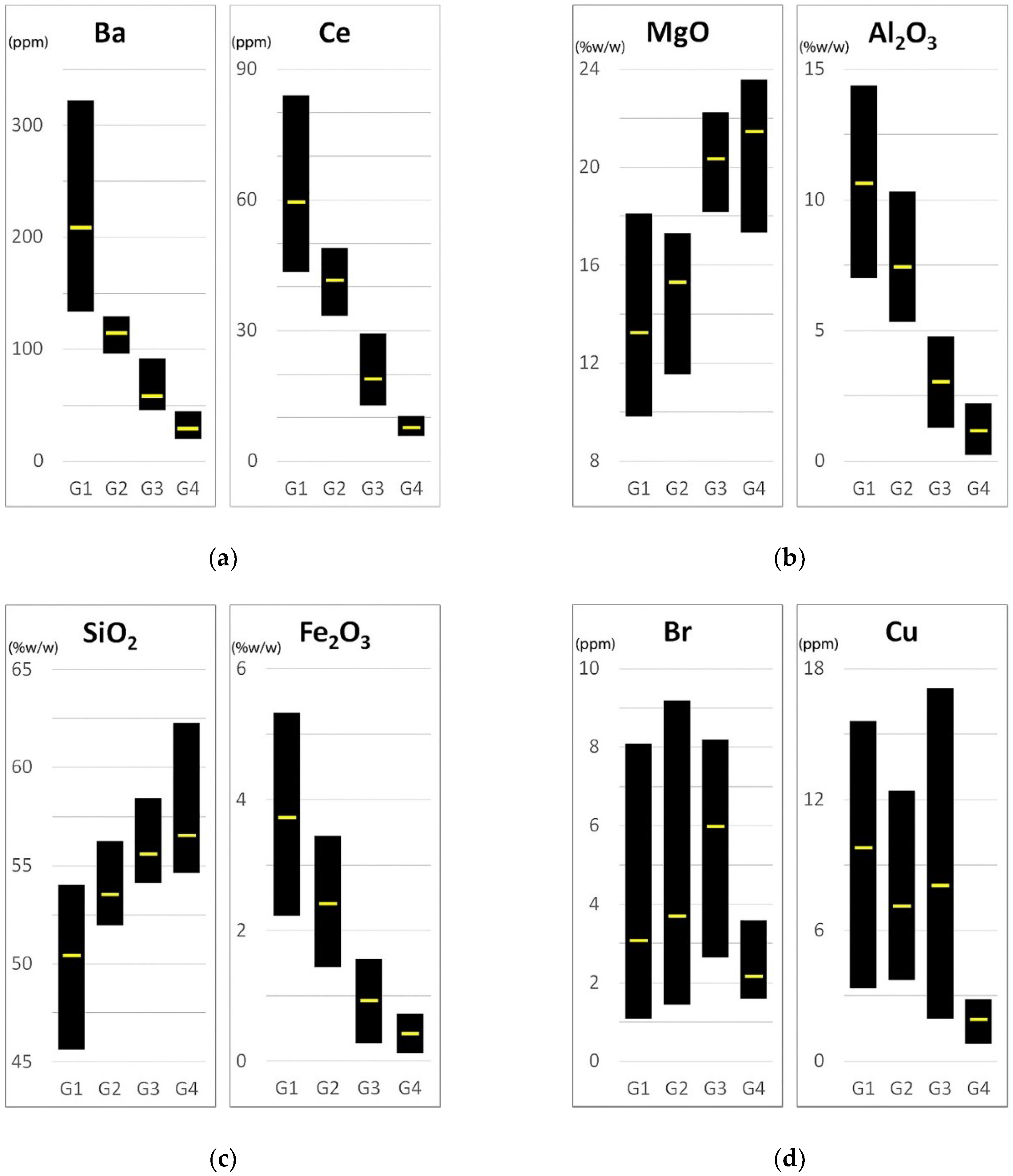
Cluster Analysis
From the Pearson r-values, obtained from the correlation of the elemental contents (of major and trace) of the studied samples (Table A2), a cluster analysis has been performed. The results of this analysis indicate that there are 4 groups of samples according to their geochemical affinities (Figure 13). For each of these groups, the maximum, minimum and average values of each of the analyzed elements have been studied in order to determine the relationship between the concentration of each element and its belonging to one geochemical group or another (Figure 14).
The samples included in Group 1 (G1) belong mostly to Unit I.1, and within this unit to lithofacies I.1-B (mudstones) and I.1-A (claystones), although two samples of lithofacies I.1-C (clay clast intrarenite) and one sample of lithofacies I.2-A (laminated lutite) are also present. Within these samples, Al2O3, and the elements positively correlated with it, have the highest concentrations (Figure 14), the opposite of MgO and SiO2. From the geochemical point of view, a relevant role is inferred from the runoff waters that introduce inherited minerals into the sedimentary environment, from which authigenic magnesian clays would be developed. This is consistent with the observed mineralogy in which Mg-smectite of saponitic composition predominates.
In Group 2 (G2), Unit I.2 samples predominate, with the majority being those belonging to the basal lithofacies I.2-A (laminated lutite) and I.2-B (brecciated/nodulized massive lutites). This group also includes a sample of clay intraclast arenite (I.1-C) and a sample of claystone (I.1-A), with an anomalous composition in these lithofacies due to its high sepiolite content. The geochemistry of this group is closer to that of Group 1 than to that of the other two (Figure 13 and Figure 14), indicating some geochemical linkage between the two. From the mineralogical point of view, the change from group G1 to G2 implies a decrease in the saponite content and a notable increase in the sepiolite of low “crystallinity” (LCS).
In Group 3 (G3) laminated lutites (I.2-A) predominate, in this case those located in the middle or at top of Unit I.2, together with some samples of lithofacies I.2-B. The chemical evolution is progressing along the lines already explained (Figure 12). However, this group presents certain geochemical anomalies that are out of normal evolution, as they have wider ranges of concentrations of some trace elements than in the other groups (see Cu in Figure 14d). The samples contained in this group belong to the transition lithofacies and to the base of the Unit II (exploitable sepiolite deposit). However, the observed geochemical conditions (Figure 14b) are closer to the overlying sepiolitic levels than to the underlying lithofacies. This indicates that the geochemical conditions are closer to those prevailing in the palustrine environment than in the mudflat.
Group 4 (G4) corresponds to the sepiolitic levels of Unit II.1 and some materials belonging to lithofacies I.2-C, present in the southernmost sections where the transition episode is not so clear. This group is the most statistically distant from the others (Figure 13), and its geochemistry shows much smaller ranges of values (especially of Al2O3 and its related elements) than the rest of the groups (Figure 14). This is related to the installation of more restricted palustrine conditions with little detrital mineral input, which favors the authigenic processes of neoformation by precipitation and limits the availability of inherited elements.
From the base at top of the lithological section, a depletion of Al2O3 and its related elements and an enrichment of MgO and SiO2 is generally observed (Figure 12 and Figure 14a–c). The exception is shown in Figure 14b, where the samples grouped in G1 and G2 show similar behavior, but different from that of G3 and G4. This division marks two distinct geochemical environments, one with the influence of Mg (G3 and G4, samples belonging to the upper lithofacies predominantly formed by authigenesis), and the other of Al (G1 and G2, samples from the lower levels, associated with inherited elements).
Additionally, the elements grouped in Figure 14a show different ranges of concentrations depending on the group to which they belong, which is related to changes in formation conditions. In general, the LILE, and especially the Ba as previously indicated, have a range of concentrations that adjust to the changes in the geochemical groups described (Figure 14a,b), as is also the case with Ce. In the TTE, a low degree of influence on the conditions of each group has been observed.
According to the FWHM value of the sepiolite, with regard to the proposed geochemical groups (Figure 14), it is observed that G1 and G2 always present values higher than 0.847 (°2Θ), while G3 and G4 are always below 0.829 (°2Θ). This is consistent with conditions of incipient sepiolite formation that has not undergone diagenetic processes of recrystallization.
4.4. Mg-Clay Minerals Formation Model
The four differentiated groups propose two differentiated geochemical environments, which condition the formation of authigenic minerals. Within Unit I, the associated G1 and G2 groups are presented in a sedimentary environment that has an available supply of aluminum-bearing clay minerals. In an environment rich in Mg and basic pH conditions, these inherited alumina precursors (mainly Al-smectite) would have favored the authigenic formation of Mg-smectite (saponite). The existence of hydrochemical changes favoring the availability of silica and a decrease in salinity and alkalinity would have favored the incipient development of low-ordering sepiolite (LCS) at the expense of Mg-smectite [13,31,42,43,44,45]. The genetic mechanism of these first sepiolite phases would be of the dissolution-precipitation type, as suggested by the textures observed in the petrographic analysis of the samples (Figure 7a,b).
The samples included in the G3 and G4 groups are associated with environments with little or no detrital influence. In this case, sepiolite is the major mineral within the clay fraction. On the basis of geochemical analyses, two genetic environments could be distinguished in the formation of sepiolite. An initial one, related to G3, in which there is still some influence of inherited (or reworked) components. The other genetic environment (G4) would be controlled by conditions with almost total absence of external inputs (low Al content and practical absence of inherited minerals, Table A1 and Table 3), with a strong influence of groundwaters (silica input). This causes a decrease in salinity-basicity and higher Si/Mg ratios, which would favor direct precipitation of sepiolite from solutions or gels [14,46,47]. Sepiolite would initially be of the LCS type, but under suitable diagenetic conditions the recrystallization is favored and then the HCS type formation. The increase in groundwater inputs means an increase in Si(OH)4, originating siliceous phases (opal-CT and quartz) when Mg is not available, and then sepiolite silicification processes or silica precipitation are common.
5. Concluding Remarks
This paper highlights the high sensitivity of Mg-clay minerals to hydrochemical variations in the sedimentary and diagenetic environment. The materials studied have a clear tendency to be geochemically grouped according to the type of water (runoff, lake and/or groundwater) involved in the formation of authigenic Mg-clays, giving rise to four geochemical groups. Based on this, the development of the studied lithofacies began with mudflat deposits from a lake margin where the sediment transported by runoff waters control the geochemistry (those associated with the G1 and G2 groups), and then moved on to a palustrine environment where groundwaters played a relevant role in the geochemistry of the authigenic minerals formed (G3 and G4 groups).
Mg-smectite was formed mainly as a result of the dissolution-precipitation of Al-smectites in a medium rich in Mg and basic pH. It is not excluded that some of the Mg-smectite was formed by direct precipitation under appropriate physicochemical conditions, even the possible coexistence of two Mg-smectites with differences in the layer charge location.
The origin of sepiolite would initially be related to the instability of Mg-smectites as a result of changes in the pH and salinity conditions of the medium. Under groundwater conditions, the formation of sepiolite is favored by direct precipitation, in dissolution or from gel-like phases, which in the palustrine environment can suffer phenomena of cementation and recrystallization during diagenesis. The type of formation explains the existence of sepiolites with different degrees of ordering (“crystallinity”). The frequent existence of drying periods sometimes with reworking of clay intraclasts and later reprecipitation justifies the existence of several generations of sepiolite.
Author Contributions
J.E.H. collected the samples, performed the mineralogical and chemical characterization, interpreted all the data and wrote the original draft of the paper. M.P. conceived and designed the study, supervised its progress and reviewed the original draft of the paper.
Funding
The work has been financed by Project CGL2015-68333-P (MINECO-FEDER, UE).
Acknowledgments
This study is part of the scientific activities of the Research Group C-144 (UAM, Geomaterials and Geological Processes). Analytical support was provided by the laboratories of the Geological Survey of Spain (IGME) and the Interdepartmental Research Service (SIdI) from Universidad Autónoma de Madrid. We especially thanks to E. Rodríguez Cañas for his assistance and skills during SEM sessions.
Conflicts of Interest
The authors declare no conflict of interest.
Appendix A

Table A1.
Chemical analysis of major elements (%w/w) of samples from Units I and II.
| Lf | Sample | SiO2 | MgO | Al2O3 | Fe2O3 | CaO | TiO2 | K2O | MnO | P2O5 | Na2O | F | PPC |
|---|---|---|---|---|---|---|---|---|---|---|---|---|---|
| II.1-A | ST-9 | 58.12 | 22.18 | 0.6 | 0.17 | 0.08 | 0.05 | 0.12 | 0.02 | - | 0.03 | - | 18.62 |
| II.1-A | BS2-I-12 | 54.64 | 22.14 | 1.53 | 0.54 | 0.37 | <0.1 | <0.4 | <0.05 | <0.045 | 0.09 | - | 19.02 |
| II.1-A | BS2-I-9 | 55.86 | 23.58 | 0.33 | 0.12 | 0.1 | <0.1 | <0.4 | <0.05 | <0.045 | 0.04 | - | 18.76 |
| I.2-A | LA-9 * | 57.25 | 18.909 | 4.45 | 1.654 | 0.552 | 0.191 | 0.767 | 0.021 | - | 0.175 | 0.51 | 15.89 |
| I.2-A | BA-16 * | 54.68 | 21.878 | 0.25 | 0.305 | 1.995 | 0.051 | 0.158 | 0.008 | - | 0.06 | 0.52 | 20.17 |
| I.2-A | BA-15 * | 58.45 | 18.155 | 4.07 | 1.094 | 0.171 | 0.177 | 0.726 | 0.049 | - | 0.192 | 0.35 | 16.56 |
| I.2-A | BA-11 * | 53.46 | 17.284 | 6.49 | 2.194 | 0.413 | 0.267 | 1.149 | 0.04 | - | 0.211 | 0.46 | 17.97 |
| I.2-A | JF-4 * | 56.33 | 22.21 | 1.29 | 0.279 | 0.807 | 0.053 | 0.133 | 0.015 | - | 0.067 | 0.68 | 18.81 |
| I.2-A | JF-2 * | 55.34 | 21.049 | 2.6 | 0.769 | 0.136 | 0.1 | 0.356 | 0.019 | - | 0.094 | 0.49 | 19.51 |
| I.2-A | COSTRA2 * | 55.88 | 20.26 | 2.98 | 1.04 | 0.24 | 0.13 | 0.59 | 0.01 | - | 0.13 | 0.44 | 18.69 |
| I.2-A | ST-10 | 52.52 | 15.06 | 8.01 | 2.61 | 0.47 | 0.32 | 1.54 | 0.03 | - | 0.28 | - | 19.13 |
| I.2-A | ST-11 | 53.15 | 15.66 | 7.59 | 2.35 | 0.47 | 0.29 | 1.33 | 0.03 | - | 0.29 | - | 18.81 |
| I.2-A | B8/9-6 * | 55.04 | 20.315 | 3.24 | 1.01 | 0.295 | 0.155 | 0.592 | 0.025 | - | 0.135 | 0.12 | 19.08 |
| I.2-A | B8/9-4 * | 51.95 | 15.55 | 6.89 | 2.152 | 0.34 | 0.286 | 1.151 | 0.044 | - | 0.255 | 0.21 | 21.18 |
| I.2-A | B8/9-3 * | 54.8 | 20.598 | 2.9 | 0.897 | 0.215 | 0.141 | 0.512 | 0.02 | - | 0.121 | 0.51 | 19.31 |
| I.2-A | BS2-I-8 | 55.19 | 20.61 | 2.77 | 0.86 | 0.12 | 0.11 | 0.51 | <0.05 | <0.045 | 0.15 | - | 18.1 |
| I.2-A | BS2-I-11 | 53.11 | 14.99 | 7.57 | 2.88 | 0.21 | 0.29 | 1.59 | <0.05 | <0.045 | 0.2 | - | 17.42 |
| I.2-A | BS2-I-5 | 52.69 | 15.02 | 8.04 | 2.66 | 0.3 | 0.27 | 1.54 | 0.05 | <0.045 | 0.2 | - | 17.74 |
| I.2-A | BS2-I-3 | 49.53 | 10.4 | 10.89 | 3.52 | 0.43 | 0.38 | 1.95 | <0.05 | <0.045 | 0.32 | - | 21.9 |
| I.2-A | BS-1B-2 | 56.27 | 16.48 | 5.34 | 1.44 | 0.26 | 0.23 | 1.29 | <0.05 | <0.045 | 0.32 | - | 17.82 |
| I.2-B | B8/9-8 * | 55.29 | 22.791 | 1.4 | 0.459 | 0.041 | 0.084 | 0.247 | 0.02 | - | 0.065 | 0.7 | 18.99 |
| I.2-B | BS2-I-7 | 54.99 | 21.2 | 2.69 | 0.85 | 0.11 | 0.1 | 0.49 | <0.05 | <0.045 | 0.11 | - | 17.98 |
| I.2-B | BS2-I-6 | 54.12 | 18.61 | 4.78 | 1.56 | 0.13 | 0.17 | 0.88 | <0.05 | <0.045 | 0.13 | - | 18.36 |
| I.2-B | BS2-I-4 | 52.87 | 11.56 | 10.31 | 3.45 | 0.28 | 0.36 | 2.1 | <0.05 | <0.045 | 0.24 | - | 17.78 |
| I.2-C | BS-1C-4 | 54.78 | 20.18 | 2.22 | 0.73 | 0.95 | <0.1 | 0.4 | <0.05 | 0.051 | 0.08 | - | 19.18 |
| I.2-C | BS-1C-2 | 54.56 | 16.38 | 6.25 | 1.77 | 0.26 | 0.26 | 1.38 | <0.05 | <0.045 | 0.31 | - | 17.38 |
| I.2-C | BS-1B-3 | 62.28 | 17.31 | 1.77 | 0.57 | 0.2 | <0.1 | 0.26 | <0.05 | <0.045 | 0.07 | - | 15.5 |
| I.1-A | LA-1 * | 52.06 | 14.42 | 10.61 | 3.98 | 1.01 | 0.4 | 1.92 | 0.047 | - | 0.31 | 0.23 | 15.1 |
| I.1-A | JF-1 * | 54.83 | 16.633 | 6.67 | 2.219 | 0.319 | 0.284 | 1.349 | 0.04 | - | 0.249 | 0.29 | 17.11 |
| I.1-A | ST-12 | 49.98 | 18.1 | 7.01 | 2.36 | 1.63 | 0.28 | 0.95 | 0.04 | - | 0.21 | - | 19.43 |
| I.1-A | B8/9-2ar * | 48.24 | 13.031 | 10.66 | 3.61 | 0.682 | 0.402 | 1.663 | 0.057 | - | 0.31 | 0.11 | 21.18 |
| I.1-B | BA-10 * | 52.48 | 11.689 | 9.85 | 3.984 | 0.686 | 0.427 | 2.634 | 0.043 | - | 0.512 | 0.13 | 17.53 |
| I.1-B | ST-13 | 50.35 | 16.56 | 8.91 | 3.2 | 0.9 | 0.38 | 1.49 | 0.05 | - | 0.28 | - | 17.81 |
| I.1-B | ST-14 | 50.83 | 13.76 | 10.15 | 3.55 | 1.1 | 0.44 | 1.84 | 0.05 | - | 0.36 | - | 17.84 |
| I.1-B | ST-15 | 51.66 | 11.76 | 12.05 | 4.45 | 0.5 | 0.57 | 2.93 | 0.04 | - | 0.37 | - | 15.64 |
| I.1-B | ST-18 | 45.65 | 10.05 | 12.76 | 4.77 | 4.17 | 0.6 | 2.67 | 0.04 | - | 0.4 | - | 18.86 |
| I.1-B | ST-19 | 50.91 | 9.83 | 14.37 | 5.33 | 0.67 | 0.74 | 3.2 | 0.05 | - | 0.57 | - | 14.28 |
| I.1-B | ST-20 | 50.71 | 11.51 | 13.59 | 5.03 | 0.7 | 0.68 | 2.84 | 0.05 | - | 0.62 | - | 14.2 |
| I.1-B | ST-21 | 50.59 | 17.03 | 8.87 | 3.32 | 0.69 | 0.42 | 1.54 | 0.05 | - | 0.28 | - | 17.18 |
| I.1-B | ST-22 | 49.84 | 16.9 | 9.28 | 3.41 | 1.01 | 0.45 | 1.65 | 0.05 | - | 0.27 | - | 17.1 |
| I.1-B | BS-1C-1 | 54.03 | 13.06 | 7.86 | 2.22 | 2.1 | 0.33 | 1.86 | <0.05 | <0.045 | 0.46 | - | 16.55 |
| I.1-C | LA-5 * | 53.88 | 6.47 | 15.71 | 5.58 | 0.88 | 0.59 | 2.83 | 0.04 | - | 0.55 | 0.22 | 13.39 |
| I.1-C | B8/9-1 * | 51.04 | 12.58 | 10.48 | 3.23 | 0.648 | 0.409 | 1.72 | 0.043 | - | 0.44 | 0.1 | 19.36 |
| I.1-C | BS2-I-1 | 50.44 | 12.13 | 12.45 | 3.94 | 0.69 | 0.46 | 2.28 | 0.05 | 0.07 | 0.48 | - | 14.5 |
| I.1-C | BS-1B-1 | 53.3 | 13.49 | 8.48 | 2.77 | 0.33 | 0.29 | 1.81 | <0.05 | <0.045 | 0.27 | - | 17.87 |
* Samples previously reported by Pozo et al. [17].
Table A2.
Pearson correlation coefficients of major and trace elements data. All data above the diagonal have a p-value less than 0.01; the values under the line showing a light brown shading have a p-value between 0.1 and 0.01; and all other values have a p-value greater than 0.1.
Table A2.
Pearson correlation coefficients of major and trace elements data. All data above the diagonal have a p-value less than 0.01; the values under the line showing a light brown shading have a p-value between 0.1 and 0.01; and all other values have a p-value greater than 0.1.
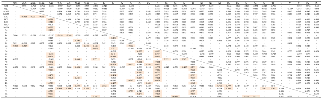
Table A3.
Summary of the maximum, minimum and mean values (ppm) of the data obtained from the trace element analyses. The highlighted average values (white text on dark gray background) show results that exceed the global average value. Elements with data below the limit of detection have not been considered.
| Lithofacies | As | Ba | Br | Ce | Co | Cr | Cs | Cu | Ga | Ge | Hf | I | La | Li | Nb | Nd | Ni | Pb | Rb | Sc | Sn | Sr | Th | U | V | Y | Zn | Zr |
|---|---|---|---|---|---|---|---|---|---|---|---|---|---|---|---|---|---|---|---|---|---|---|---|---|---|---|---|---|
| Global | ||||||||||||||||||||||||||||
| Max. | 17.5 | 322.6 | 44.7 | 83.9 | 9.9 | 33.3 | 7.4 | 17.1 | 23.2 | 4.0 | 4.9 | 10.1 | 37.3 | 207.0 | 19.3 | 35.7 | 19.0 | 19.0 | 178.5 | 12.8 | 11.0 | 161.6 | 18.0 | 2.5 | 91.1 | 31.0 | 89.3 | 120.7 |
| Min. | 0.8 | 20.1 | 1.1 | 5.9 | 1.2 | 3.2 | 7.3 | 0.8 | 1.3 | 0.6 | 3.2 | 5.9 | 0.9 | 45.0 | 1.3 | 4.3 | 1.8 | 1.9 | 3.4 | 1.0 | 2.2 | 5.0 | 0.9 | 0.6 | 21.1 | 1.9 | 2.9 | 5.9 |
| Mean | 4.8 | 126.8 | 5.3 | 42.4 | 4.9 | 13.1 | 7.4 | 8.0 | 11.4 | 2.2 | 4.0 | 7.8 | 19.3 | 99.3 | 9.0 | 20.4 | 8.1 | 9.4 | 74.1 | 7.1 | 5.3 | 63.3 | 9.4 | 1.4 | 46.9 | 14.0 | 41.2 | 50.7 |
| Samples | 27 | 39 | 27 | 35 | 23 | 36 | 2 | 37 | 36 | 32 | 4 | 3 | 36 | 8 | 37 | 30 | 22 | 39 | 37 | 30 | 30 | 37 | 36 | 8 | 41 | 38 | 42 | 37 |
| II1A | ||||||||||||||||||||||||||||
| Max. | 2.8 | 28.5 | 3.6 | 4.9 | 2.0 | 1.9 | 3.8 | 7.3 | 5.9 | 1.3 | 2.9 | 12.7 | 10.3 | 31.9 | 2.1 | 8.9 | 11.3 | |||||||||||
| Min. | 2.8 | 20.1 | 1.6 | 4.9 | 2.0 | 1.3 | 2.1 | 7.3 | 5.9 | 1.3 | 2.9 | 3.4 | 5.0 | 22.9 | 1.9 | 2.9 | 5.9 | |||||||||||
| Mean | 2.8 | 23.0 | 2.4 | 4.9 | 2.0 | 1.6 | 2.8 | 7.3 | 5.9 | 1.3 | 2.9 | 7.8 | 8.4 | 27.4 | 2.0 | 6.0 | 8.6 | |||||||||||
| Samples | 1 | 3 | 3 | 0 | 0 | 1 | 0 | 1 | 2 | 3 | 0 | 1 | 1 | 0 | 1 | 0 | 0 | 1 | 3 | 0 | 0 | 3 | 0 | 0 | 2 | 2 | 3 | 3 |
| I2A | ||||||||||||||||||||||||||||
| Max. | 5.9 | 160.0 | 8.2 | 48.9 | 5.0 | 33.3 | 7.3 | 17.1 | 18.2 | 3.6 | 3.9 | 10.1 | 28.0 | 118.0 | 12.9 | 22.6 | 17.3 | 14.4 | 117.8 | 8.5 | 7.4 | 86.5 | 14.3 | 2.5 | 91.1 | 21.4 | 61.4 | 94.2 |
| Min. | 0.8 | 21.0 | 1.5 | 7.0 | 1.2 | 3.2 | 7.3 | 3.9 | 4.0 | 1.4 | 3.9 | 10.1 | 0.9 | 45.0 | 3.0 | 6.5 | 1.8 | 1.9 | 24.6 | 1.0 | 2.2 | 15.9 | 0.9 | 0.6 | 25.5 | 3.0 | 14.0 | 24.6 |
| Mean | 2.8 | 93.5 | 5.3 | 32.1 | 3.1 | 13.9 | 7.3 | 8.6 | 9.5 | 2.2 | 3.9 | 10.1 | 14.4 | 78.3 | 7.2 | 16.5 | 7.8 | 7.5 | 62.4 | 5.1 | 4.3 | 47.0 | 6.9 | 1.2 | 44.9 | 11.8 | 33.5 | 48.4 |
| Samples | 13 | 13 | 12 | 13 | 6 | 14 | 1 | 14 | 12 | 12 | 1 | 1 | 12 | 6 | 13 | 11 | 13 | 15 | 12 | 11 | 12 | 12 | 15 | 5 | 16 | 13 | 16 | 12 |
| I2B | ||||||||||||||||||||||||||||
| Max. | 3.8 | 120.9 | 44.7 | 42.2 | 3.3 | 16.5 | 7.4 | 4.9 | 17.2 | 4.0 | 5.9 | 25.3 | 11.6 | 21.1 | 13.9 | 10.9 | 107.6 | 9.5 | 6.9 | 55.5 | 10.8 | 0.9 | 57.6 | 13.3 | 49.9 | 46.3 | ||
| Min. | 1.5 | 32.9 | 1.6 | 5.9 | 3.3 | 4.0 | 7.4 | 0.8 | 2.7 | 2.0 | 5.9 | 1.2 | 1.3 | 4.3 | 2.9 | 2.5 | 12.3 | 2.0 | 2.4 | 9.0 | 1.4 | 0.9 | 21.1 | 3.9 | 7.9 | 22.0 | ||
| Mean | 3.1 | 64.6 | 13.2 | 22.7 | 3.3 | 9.9 | 7.4 | 2.9 | 7.8 | 2.8 | 5.9 | 13.2 | 5.3 | 11.7 | 7.1 | 6.4 | 48.8 | 5.8 | 3.9 | 25.1 | 5.2 | 0.9 | 36.0 | 7.4 | 25.3 | 29.4 | ||
| Samples | 4 | 4 | 4 | 4 | 1 | 4 | 1 | 4 | 4 | 4 | 0 | 1 | 4 | 0 | 4 | 3 | 3 | 4 | 4 | 2 | 3 | 4 | 4 | 1 | 4 | 4 | 4 | 4 |
| I2C | ||||||||||||||||||||||||||||
| Max. | 3.9 | 115.6 | 2.0 | 41.3 | 3.0 | 4.7 | 3.7 | 8.5 | 3.6 | 8.7 | 7.0 | 11.7 | 3.1 | 6.3 | 63.1 | 5.1 | 3.1 | 36.1 | 8.4 | 71.0 | 10.6 | 39.8 | 70.9 | |||||
| Min. | 3.9 | 37.3 | 1.5 | 10.4 | 2.8 | 4.7 | 2.9 | 2.7 | 2.4 | 5.7 | 1.8 | 11.7 | 3.1 | 2.1 | 14.5 | 5.1 | 3.1 | 16.3 | 2.0 | 36.5 | 4.3 | 7.9 | 14.7 | |||||
| Mean | 3.9 | 65.9 | 1.7 | 25.8 | 2.9 | 4.7 | 3.3 | 5.0 | 3.2 | 7.1 | 3.7 | 11.7 | 3.1 | 4.2 | 32.7 | 5.1 | 3.1 | 24.3 | 5.2 | 52.6 | 6.9 | 19.9 | 35.2 | |||||
| Samples | 1 | 3 | 3 | 2 | 2 | 1 | 0 | 2 | 3 | 3 | 0 | 0 | 3 | 0 | 3 | 1 | 1 | 3 | 3 | 1 | 1 | 3 | 2 | 0 | 3 | 3 | 3 | 3 |
| I1A | ||||||||||||||||||||||||||||
| Max. | 17.5 | 208.0 | 9.2 | 63.1 | 3.7 | 20.0 | 12.4 | 17.9 | 2.7 | 21.5 | 117.0 | 16.7 | 33.3 | 19.0 | 13.0 | 108.4 | 9.0 | 8.0 | 161.6 | 16.4 | 2.5 | 73.0 | 31.0 | 68.1 | 65.3 | |||
| Min. | 3.5 | 118.3 | 1.6 | 33.5 | 3.7 | 6.5 | 4.0 | 10.0 | 0.6 | 10.7 | 117.0 | 6.8 | 14.9 | 18.0 | 8.1 | 62.7 | 4.7 | 4.2 | 40.4 | 8.1 | 1.6 | 31.3 | 10.4 | 38.8 | 48.1 | |||
| Mean | 10.5 | 153.2 | 5.4 | 46.7 | 3.7 | 13.8 | 8.7 | 13.0 | 1.7 | 15.7 | 117.0 | 10.3 | 21.7 | 18.5 | 10.2 | 80.5 | 6.2 | 5.7 | 102.1 | 11.6 | 2.1 | 52.4 | 17.4 | 50.3 | 55.7 | |||
| Samples | 2 | 3 | 2 | 3 | 1 | 3 | 0 | 3 | 3 | 2 | 0 | 0 | 3 | 1 | 3 | 3 | 2 | 3 | 3 | 3 | 3 | 3 | 3 | 2 | 3 | 3 | 3 | 3 |
| I1B | ||||||||||||||||||||||||||||
| Max. | 11.8 | 322.6 | 1.5 | 76.0 | 9.9 | 22.6 | 15.6 | 23.2 | 2.1 | 4.9 | 37.3 | 207.0 | 19.3 | 31.5 | 4.1 | 19.0 | 178.5 | 12.8 | 11.0 | 123.8 | 18.0 | 63.6 | 26.7 | 89.3 | 111.7 | |||
| Min. | 6.8 | 175.0 | 1.1 | 47.3 | 3.0 | 6.3 | 3.3 | 11.1 | 1.1 | 4.9 | 20.2 | 207.0 | 9.8 | 20.6 | 4.1 | 10.6 | 86.4 | 6.9 | 4.5 | 68.5 | 11.0 | 45.1 | 17.4 | 44.9 | 52.9 | |||
| Mean | 9.7 | 227.2 | 1.3 | 58.3 | 7.1 | 15.1 | 10.3 | 17.6 | 1.4 | 4.9 | 30.4 | 207.0 | 14.1 | 25.5 | 4.1 | 14.3 | 125.7 | 9.7 | 7.1 | 104.6 | 14.1 | 51.4 | 20.6 | 68.2 | 71.6 | |||
| Samples | 4 | 10 | 2 | 10 | 10 | 10 | 0 | 10 | 9 | 7 | 1 | 0 | 10 | 1 | 10 | 9 | 1 | 10 | 9 | 10 | 9 | 9 | 9 | 0 | 10 | 10 | 10 | 9 |
| I1C | ||||||||||||||||||||||||||||
| Max. | 10.6 | 189.2 | 2.4 | 83.9 | 4.5 | 11.9 | 9.6 | 18.2 | 2.4 | 3.9 | 34.6 | 13.2 | 35.7 | 7.1 | 16.5 | 114.2 | 9.8 | 8.1 | 148.6 | 17.9 | 81.7 | 28.7 | 72.0 | 120.7 | ||||
| Min. | 3.5 | 118.1 | 2.4 | 48.9 | 2.9 | 10.4 | 7.3 | 13.6 | 2.4 | 3.2 | 22.4 | 9.3 | 20.1 | 3.6 | 9.0 | 88.3 | 7.3 | 5.4 | 52.9 | 9.9 | 41.3 | 13.0 | 44.1 | 54.3 | ||||
| Mean | 7.1 | 157.5 | 2.4 | 67.6 | 3.8 | 11.1 | 8.8 | 16.1 | 2.4 | 3.5 | 29.9 | 11.5 | 30.4 | 5.3 | 13.0 | 101.4 | 8.6 | 6.7 | 110.2 | 14.7 | 58.9 | 22.3 | 60.9 | 78.8 | ||||
| Samples | 2 | 3 | 1 | 3 | 3 | 3 | 0 | 3 | 3 | 1 | 2 | 0 | 3 | 0 | 3 | 3 | 2 | 3 | 3 | 3 | 2 | 3 | 3 | 0 | 3 | 3 | 3 | 3 |
Table A4.
Summary of the maximum, minimum and mean values of the data obtained from the normalization of trace elements with the Upper Continental Crust (UCC) composition. The highlighted average values (bold on a blue background) indicate enrichment with respect to the UCC.
Table A4.
Summary of the maximum, minimum and mean values of the data obtained from the normalization of trace elements with the Upper Continental Crust (UCC) composition. The highlighted average values (bold on a blue background) indicate enrichment with respect to the UCC.
| Lithofacies | As | Ba | Br | Ce | Co | Cr | Cs | Cu | Ga | Ge | Hf | I | La | Li | Nb | Nd | Ni | Pb | Rb | Sc | Sn | Sr | Th | U | V | Y | Zn | Zr |
|---|---|---|---|---|---|---|---|---|---|---|---|---|---|---|---|---|---|---|---|---|---|---|---|---|---|---|---|---|
| Global | ||||||||||||||||||||||||||||
| Max. | 3.65 | 0.51 | 27.94 | 1.33 | 0.57 | 0.36 | 1.51 | 0.61 | 1.33 | 2.86 | 0.92 | 7.22 | 1.20 | 8.63 | 1.61 | 1.32 | 0.40 | 1.12 | 2.13 | 0.91 | 5.24 | 0.51 | 1.71 | 0.93 | 0.94 | 1.48 | 1.33 | 0.63 |
| Min. | 0.17 | 0.03 | 0.68 | 0.09 | 0.07 | 0.03 | 1.49 | 0.03 | 0.07 | 0.43 | 0.60 | 4.22 | 0.03 | 1.88 | 0.11 | 0.16 | 0.04 | 0.11 | 0.04 | 0.07 | 1.05 | 0.02 | 0.09 | 0.22 | 0.22 | 0.09 | 0.04 | 0.03 |
| Mean | 1.00 | 0.20 | 3.34 | 0.67 | 0.29 | 0.14 | 1.50 | 0.29 | 0.65 | 1.61 | 0.75 | 5.54 | 0.62 | 4.14 | 0.75 | 0.76 | 0.17 | 0.55 | 0.88 | 0.51 | 2.54 | 0.20 | 0.90 | 0.51 | 0.48 | 0.67 | 0.62 | 0.26 |
| Samples | 27 | 39 | 27 | 35 | 23 | 36 | 2 | 37 | 36 | 32 | 4 | 3 | 36 | 8 | 37 | 30 | 22 | 39 | 37 | 30 | 30 | 37 | 36 | 8 | 41 | 38 | 42 | 37 |
| II1A | ||||||||||||||||||||||||||||
| Max. | 0.58 | 0.05 | 2.25 | 0.05 | 0.07 | 0.11 | 2.73 | 5.19 | 0.19 | 0.11 | 0.17 | 0.15 | 0.03 | 0.33 | 0.10 | 0.13 | 0.06 | |||||||||||
| Min. | 0.58 | 0.03 | 0.99 | 0.05 | 0.07 | 0.07 | 1.50 | 5.19 | 0.19 | 0.11 | 0.17 | 0.04 | 0.02 | 0.24 | 0.09 | 0.04 | 0.03 | |||||||||||
| Mean | 0.58 | 0.04 | 1.49 | 0.05 | 0.07 | 0.09 | 2.03 | 5.19 | 0.19 | 0.11 | 0.17 | 0.09 | 0.03 | 0.28 | 0.10 | 0.09 | 0.04 | |||||||||||
| Samples | 1 | 3 | 3 | 0 | 0 | 1 | 0 | 1 | 2 | 3 | 0 | 1 | 1 | 0 | 1 | 0 | 0 | 1 | 3 | 0 | 0 | 3 | 0 | 0 | 2 | 2 | 3 | 3 |
| I2A | ||||||||||||||||||||||||||||
| Max. | 1.23 | 0.25 | 5.13 | 0.78 | 0.29 | 0.36 | 1.49 | 0.61 | 1.04 | 2.60 | 0.73 | 7.22 | 0.90 | 4.92 | 1.08 | 0.84 | 0.37 | 0.84 | 1.40 | 0.61 | 3.54 | 0.27 | 1.37 | 0.93 | 0.94 | 1.02 | 0.92 | 0.49 |
| Min. | 0.17 | 0.03 | 0.94 | 0.11 | 0.07 | 0.03 | 1.49 | 0.14 | 0.23 | 0.96 | 0.73 | 7.22 | 0.03 | 1.88 | 0.25 | 0.24 | 0.04 | 0.11 | 0.29 | 0.07 | 1.05 | 0.05 | 0.09 | 0.22 | 0.26 | 0.14 | 0.21 | 0.13 |
| Mean | 0.58 | 0.15 | 3.31 | 0.51 | 0.18 | 0.15 | 1.49 | 0.31 | 0.54 | 1.60 | 0.73 | 7.22 | 0.46 | 3.26 | 0.60 | 0.61 | 0.17 | 0.44 | 0.74 | 0.36 | 2.03 | 0.15 | 0.65 | 0.45 | 0.46 | 0.56 | 0.50 | 0.25 |
| Samples | 13 | 13 | 12 | 13 | 6 | 14 | 1 | 14 | 12 | 12 | 1 | 1 | 12 | 6 | 13 | 11 | 13 | 15 | 12 | 11 | 12 | 12 | 15 | 5 | 16 | 13 | 16 | 12 |
| I2B | ||||||||||||||||||||||||||||
| Max. | 0.80 | 0.19 | 27.94 | 0.67 | 0.19 | 0.18 | 1.51 | 0.17 | 0.98 | 2.86 | 4.22 | 0.82 | 0.97 | 0.78 | 0.30 | 0.64 | 1.28 | 0.68 | 3.30 | 0.17 | 1.03 | 0.33 | 0.59 | 0.64 | 0.74 | 0.24 | ||
| Min. | 0.31 | 0.05 | 1.02 | 0.09 | 0.19 | 0.04 | 1.51 | 0.03 | 0.15 | 1.46 | 4.22 | 0.04 | 0.11 | 0.16 | 0.06 | 0.15 | 0.15 | 0.14 | 1.12 | 0.03 | 0.13 | 0.33 | 0.22 | 0.19 | 0.12 | 0.11 | ||
| Mean | 0.65 | 0.10 | 8.23 | 0.36 | 0.19 | 0.11 | 1.51 | 0.10 | 0.45 | 2.03 | 4.22 | 0.43 | 0.44 | 0.43 | 0.15 | 0.38 | 0.58 | 0.41 | 1.85 | 0.08 | 0.49 | 0.33 | 0.37 | 0.35 | 0.38 | 0.15 | ||
| Samples | 4 | 4 | 4 | 4 | 1 | 4 | 1 | 4 | 4 | 4 | 0 | 1 | 4 | 0 | 4 | 3 | 3 | 4 | 4 | 2 | 3 | 4 | 4 | 1 | 4 | 4 | 4 | 4 |
| I2C | ||||||||||||||||||||||||||||
| Max. | 0.82 | 0.18 | 1.25 | 0.66 | 0.17 | 0.05 | 0.13 | 0.48 | 2.60 | 0.28 | 0.58 | 0.43 | 0.07 | 0.37 | 0.75 | 0.37 | 1.48 | 0.11 | 0.80 | 0.73 | 0.50 | 0.59 | 0.37 | |||||
| Min. | 0.82 | 0.06 | 0.91 | 0.16 | 0.16 | 0.05 | 0.10 | 0.16 | 1.69 | 0.18 | 0.15 | 0.43 | 0.07 | 0.12 | 0.17 | 0.37 | 1.48 | 0.05 | 0.19 | 0.38 | 0.20 | 0.12 | 0.08 | |||||
| Mean | 0.82 | 0.11 | 1.05 | 0.41 | 0.17 | 0.05 | 0.12 | 0.28 | 2.28 | 0.23 | 0.31 | 0.43 | 0.07 | 0.25 | 0.39 | 0.37 | 1.48 | 0.08 | 0.49 | 0.54 | 0.33 | 0.30 | 0.18 | |||||
| Samples | 1 | 3 | 3 | 2 | 2 | 1 | 0 | 2 | 3 | 3 | 0 | 0 | 3 | 0 | 3 | 1 | 1 | 3 | 3 | 1 | 1 | 3 | 2 | 0 | 3 | 3 | 3 | 3 |
| I1A | ||||||||||||||||||||||||||||
| Max. | 3.65 | 0.33 | 5.75 | 1.00 | 0.21 | 0.22 | 0.44 | 1.02 | 1.93 | 0.69 | 4.88 | 1.39 | 1.23 | 0.40 | 0.76 | 1.29 | 0.64 | 3.81 | 0.51 | 1.56 | 0.93 | 0.75 | 1.48 | 1.02 | 0.34 | |||
| Min. | 0.73 | 0.19 | 1.00 | 0.53 | 0.21 | 0.07 | 0.14 | 0.57 | 0.43 | 0.35 | 4.88 | 0.57 | 0.55 | 0.38 | 0.48 | 0.75 | 0.34 | 2.00 | 0.13 | 0.77 | 0.59 | 0.32 | 0.50 | 0.58 | 0.25 | |||
| Mean | 2.19 | 0.24 | 3.38 | 0.74 | 0.21 | 0.15 | 0.31 | 0.74 | 1.18 | 0.51 | 4.88 | 0.86 | 0.80 | 0.39 | 0.60 | 0.96 | 0.45 | 2.70 | 0.32 | 1.10 | 0.76 | 0.54 | 0.83 | 0.75 | 0.29 | |||
| Samples | 2 | 3 | 2 | 3 | 1 | 3 | 0 | 3 | 3 | 2 | 0 | 0 | 3 | 1 | 3 | 3 | 2 | 3 | 3 | 3 | 3 | 3 | 3 | 2 | 3 | 3 | 3 | 3 |
| I1B | ||||||||||||||||||||||||||||
| Max. | 2.46 | 0.51 | 0.94 | 1.21 | 0.57 | 0.25 | 0.56 | 1.33 | 1.49 | 0.92 | 1.20 | 8.63 | 1.61 | 1.17 | 0.09 | 1.12 | 2.13 | 0.91 | 5.24 | 0.39 | 1.71 | 0.66 | 1.27 | 1.33 | 0.58 | |||
| Min. | 1.41 | 0.28 | 0.68 | 0.75 | 0.17 | 0.07 | 0.12 | 0.64 | 0.79 | 0.92 | 0.65 | 8.63 | 0.82 | 0.76 | 0.09 | 0.62 | 1.03 | 0.49 | 2.16 | 0.21 | 1.05 | 0.46 | 0.83 | 0.67 | 0.27 | |||
| Mean | 2.02 | 0.36 | 0.81 | 0.92 | 0.41 | 0.16 | 0.37 | 1.00 | 1.03 | 0.92 | 0.98 | 8.63 | 1.17 | 0.95 | 0.09 | 0.84 | 1.50 | 0.69 | 3.37 | 0.33 | 1.34 | 0.53 | 0.98 | 1.02 | 0.37 | |||
| Samples | 4 | 10 | 2 | 10 | 10 | 10 | 0 | 10 | 9 | 7 | 1 | 0 | 10 | 1 | 10 | 9 | 1 | 10 | 9 | 10 | 9 | 9 | 9 | 0 | 10 | 10 | 10 | 9 |
| I1C | ||||||||||||||||||||||||||||
| Max. | 2.21 | 0.30 | 1.47 | 1.33 | 0.26 | 0.13 | 0.34 | 1.04 | 1.69 | 0.73 | 1.12 | 1.10 | 1.32 | 0.15 | 0.97 | 1.36 | 0.70 | 3.86 | 0.46 | 1.70 | 0.84 | 1.37 | 1.07 | 0.63 | ||||
| Min. | 0.74 | 0.19 | 1.47 | 0.78 | 0.17 | 0.11 | 0.26 | 0.78 | 1.69 | 0.60 | 0.72 | 0.78 | 0.75 | 0.08 | 0.53 | 1.05 | 0.52 | 2.56 | 0.17 | 0.94 | 0.43 | 0.62 | 0.66 | 0.28 | ||||
| Mean | 1.47 | 0.25 | 1.47 | 1.07 | 0.22 | 0.12 | 0.31 | 0.92 | 1.69 | 0.67 | 0.96 | 0.96 | 1.13 | 0.11 | 0.76 | 1.21 | 0.62 | 3.21 | 0.34 | 1.40 | 0.61 | 1.06 | 0.91 | 0.41 | ||||
| Samples | 2 | 3 | 1 | 3 | 3 | 3 | 0 | 3 | 3 | 1 | 2 | 0 | 3 | 0 | 3 | 3 | 2 | 3 | 3 | 3 | 2 | 3 | 3 | 0 | 3 | 3 | 3 | 3 |
References
- Calvo, J.P.; Blanc-Valleron, M.M.; Rodríguez-Aranda, J.P.; Rouchy, J.M.; Sanz, M.E. Authigenic clay minerals in continental evaporitic environments. In Palaeoweathering, Palaeosurfaces and Related Continental Deposits; Thiry, M., Simon-Coincon, R., Eds.; Special Publications of the International Association of Sedimentologists: Oxford, UK, 1999; Volume 27, pp. 129–151. [Google Scholar]
- Cowardin, L.M.; Carter, V.; Golet, F.C.; LaRoe, E.T. Classification of Wetlands and Deepwater Habitats of the United States. In Office of Biological Services, Fish and Wildlife Service, U.S. Dept. of the Interior, Washington, D.C.; Office of Biological Services, Fish and Wildlife Service, U.S. Dept. of the Interior: Washington, DC, USA, 1979. [Google Scholar]
- Jones, B.F. Clay mineral diagenesis in lacustrine sediments. US Geol. Surv. Bull. 1986, 1578, 291–300. [Google Scholar]
- Ordoñez, S.; Calvo, J.P.; García del Cura, M.A.; Alonso Zarza, A.M.; Hoyos, M. Sedimentology of sodium sulphate deposits and special clays from the Tertiary Madrid Basin (Spain). In Lacustrine Facies Analysis; Anadón, P., Cabrera, L., Kelts, K., Eds.; Spec. Publ. Int. Assoc. Sedimentol. Blackwell Sci. Publ. Oxf.: Oxford, UK, 1991; Volume 13, pp. 39–55. [Google Scholar]
- Pozo, M.; Calvo, J.P. Madrid Basin (Spain): A natural lab for the formation and evolution of magnesian clay minerals. In Magnesian Clays: Characterization, Origin and Applications; Pozo, M., Galán, E., Eds.; AIPEA Educational Series, Pub. No. 2; Digilabs: Bari, Italy, 2015; pp. 229–281. [Google Scholar]
- Clauer, N.; Fallick, A.E.; Galán, E.; Pozo, P.; Taylor, C. Varied crystallization conditions for neogene sepiolite and associated Mg-Clays from Madrid Basin (Spain) traced by oxygen and hidrogen isotope geochemistry. Geochim. Cosmochim. Acta 2012, 94, 181–198. [Google Scholar] [CrossRef]
- Alonso-Zarza, A.M.; Calvo, J.P. Tajo Basin. In The Geology of Spain; Gibbons, W., Moreno, T., Eds.; The Geological Society: London, UK, 2002; pp. 315–320. [Google Scholar]
- Calvo, J.P.; Jones, B.F.; Bustillo, M.; Fort, R.; Alonso-Zarza, A.M.; Kendall, C. Sedimentology and geochemistry of carbonates from lacustrine sequences in the Madrid Basin, Central Spain. Chem. Geol. 1995, 123, 173–191. [Google Scholar] [CrossRef]
- Cañaveras, J.C.; Calvo, J.P.; Hoyos, M.; Ordóñez, S. Paleomorphologic features of a Intra-Vallesian Paleokarst, Tertiary Madrid Basin. Significance of Paleokarstic Surfaces in Continental Basin Analysis; Friend, P., Dabrio, C.J., Eds.; Cambridge University Press: Cambridge, UK, 1996; pp. 278–284. [Google Scholar]
- Rodríguez-Aranda, J.P.; Calvo, J.P.; Sanz-Montero, M.E. Lower Miocene gypsum palaeokarst in the Madrid Basin (central Spain): Dissolution diagenesis, morphological relics and karst-end products. Sedimentology 2002, 49, 1385–1400. [Google Scholar]
- Pozo, M.; Casas, J. Distribucion y caracterizacion de litofacies en el yacimiento de arcillas magnesicas de Esquivias (Neogeno de la Cuenca de Madrid). Bol. Geol. Min. 1995, 106, 65–82. [Google Scholar]
- Cuevas, J.; Vigil de la Villa, R.; Ramírez, S.; Petit, S.; Meunier, A.; Leguey, S. Chemistry of Mg smectites in lacustrine sediments from the Vicálvaro sepiolite deposit, Madrid Neogene Basin (Spain). Clays Clay Miner. 2003, 51, 457–472. [Google Scholar] [CrossRef]
- Pozo, M. Origin and evolution of magnesium clays in lacustrine environments: Sedimentology and geochemical pathways. In First Latin-American Clay Conference. Invited Lectures. Proceedings Vol. 1.; Gomes, C.S.F., Ed.; Funchal: Madeira, Portugal, 2000; pp. 117–133. [Google Scholar]
- Galán, E.; Pozo, M. Palygorskite and sepiolite deposits in continental environments. Description, genetic patterns and sedimentary settings. In Developments in Palygorskite–Sepiolite Research. A New Outlook on These Nanomaterials. Developments in Clay Science; Galán, E., Singer, A., Eds.; Elsevier: Amsterdam, The Netherlands, 2011; Volume 3, pp. 125–173. [Google Scholar]
- Galán, E.; Pozo, M. The mineralogy, geology, and main occurrences of sepiolite and palygorskite clays. In Natural Mineral Nanotubes; Apple Academic Press: New York, NY, USA, 2015; pp. 117–130. ISBN 978-1-77188-056-5. [Google Scholar]
- Pozo, M.; Galán, E. Magnesian clay deposits: Mineralogy and origin. In Magnesian Clays: Characterization, Origin and Applications; Pozo, M., Galán, E., Eds.; AIPEA Educational Series, Pub. No. 2; Digilabs: Bari Italy, 2015; pp. 175–228. [Google Scholar]
- Pozo, M.; Calvo, J.P.; Pozo, E.; Moreno, A. Genetic constraints on crystallinity, thermal behaviour and surface area of sepiolite from the Cerro de los Batallones deposits (Madrid Basin, Spain). Appl. Clay Sci. 2014, 91–92, 30–45. [Google Scholar] [CrossRef]
- Pozo, M.; Calvo, J.P.; Silva, P.G.; Morales, J.; Peláez-Campomanes, P.; Nieto, M. Geología del sistema de yacimientos de mamíferos miocenos del Cerro de los Batallones, Cuenca de Madrid. Geogaceta 2004, 35, 143–146. [Google Scholar]
- Bustillo, M.A.; Bustillo, M. Miocene silcretes in argillaceous playa deposits, Madrid Basin, Spain: Petrological and geochemical features. Sedimentology 2000, 47, 1023–1037. [Google Scholar] [CrossRef]
- Bustillo, M.A.; Alonso-Zarza, A.M. Overlapping of pedogenesis andmeteoric diagenesis in distal alluvial and shallow lacustrine deposits in the Miocene Madrid Basin, Spain. Sediment. Geol. 2007, 198, 255–271. [Google Scholar] [CrossRef] [Green Version]
- Chung, F.H. Quantitative Interpretation of X-ray Diffraction Patterns of Mixtures. I. Matrix-Flushing Method for Quantitative Multicomponent Analysis. J. Appl. Cryst. 1974, 7, 519–525. [Google Scholar] [CrossRef]
- Schultz, L.G. Quantitative Interpretation of Mineralogical Composition from X-ray and Chemical Data for the Pierre Shale. Geol. Surv. Prof. Pap. 1964. Available online: https://pubs.usgs.gov/pp/0391c/report.pdf (accessed on 20 September 2018).
- Van der Marel, H.W. Quantitative analysis of clay minerals and their admixtures. Contrib. Miner. Pet. 1966, 12, 96–138. [Google Scholar] [CrossRef]
- Sánchez del Río, M.; García-Romero, E.; Suárez, M.; Da Silva, I.; Fuentes-Montero, L.; Martínez-Criado, G. Variability in sepiolite: Diffraction studies. Am. Miner. 2011, 96, 1443–1454. [Google Scholar] [CrossRef]
- Christidis, G.E.; Koutsopoulou, E. A simple approach to the identification of trioctahedral smectites by X-ray diffraction. Clay Miner. 2013, 48, 687–696. [Google Scholar] [CrossRef]
- Rudnick, R.L.; Gao, S. Composition of the Continental Crust. In Treatise on Geochemistry; Holland, H.D., Turekian, K.K., Eds.; Elsevier: Amsterdam, The Netherlands, 2003; Volume 3. [Google Scholar]
- Whitney, D.L.; Evans, B.W. Abbreviations for name of rock-forming minerals. Am. Miner. 2010, 95, 185–187. [Google Scholar] [CrossRef]
- Calvo, J.P.; Pozo, M.; Silva, P.G.; Morales, J. Pattern of sedimentary infilling of fossil mammal traps formed in pseudokarst at Cerro de los Batallones, Madrid Basin, Central Spain. Sedimentology 2013, 60, 1681–1708. [Google Scholar] [CrossRef]
- Galán, E.; Aparicio, P. Methodology for the identification and characterization of magnesian clays. In Magnesian Clays: Characterization, Origin and Applications; Pozo, M., Galán, E., Eds.; AIPEA Educational Series, Pub. No. 2; Digilabs: Bari, Italy, 2015; pp. 63–121. [Google Scholar]
- Guggenheim, S. Introduction to Mg-Rich clay minerals: Structure and composition. In Magnesian Clays: Characterization, Origin and Applications; Pozo, M., Galán, E., Eds.; AIPEA Educational Series, Pub. No. 2; Digilabs: Bari, Italy, 2015; pp. 1–62. [Google Scholar]
- Pozo, M.; Casas, J.C. Origin of kerolite and associated Mg clays in palustrine–lacustrine environments. The Esquivias deposit (Neogene Madrid Basin, Spain). Clay Miner. 1999, 34, 395–418. [Google Scholar] [CrossRef]
- Yalçin, H.; Bozkaya, O. Sepiolite–palygorskite occurrences in Turkey. In Developments in Palygorskite–Sepiolite Research. A New Outlook on These Nanomaterials. Developments in Clay Science; Galán, E., Singer, A., Eds.; Elsevier: Amsterdam, The Netherlands, 2011; Volume 3, pp. 175–200. [Google Scholar]
- Ece, Ö.I.; Çoban, F. Geology, occurrence, and genesis of Eskisehir sepiolites, Turkey. Clays Clay Miner. 1994, 42, 81–92. [Google Scholar] [CrossRef]
- Hay, R.L.; Hughes, R.E.; Kyser, T.K.; Glass, H.D.; Lin, J. Magnesium-rich clays of the Meerschaum mines in the Amboseli Basin, Tanzania and Kenya. Clays Clay Miner. 1995, 43, 455–466. [Google Scholar] [CrossRef]
- Tosca, N. Geochemical pathways to Mg-silicate formation. In Magnesian Clays: Characterization, Origin and Applications; Pozo, M., Galán, E., Eds.; AIPEA Educational Series, Pub. No. 2; Digilabs: Bari, Italy, 2015; pp. 283–330. [Google Scholar]
- Pozo, M.; Leguey, S.; Medina, J.A. Sepiolite and palygorskite genesis in carbonate lacustrine environments. (Duero Basin, Spain). Chem. Geol. 1990, 84, 290–291. [Google Scholar] [CrossRef]
- Torres-Ruíz, J.; López-Galindo, A.; González-López, J.M.; Delgado, A. Geochemistry of Spanish sepiolite-palygorskite deposits: Genetic considerations based on trace elements and isotopes. Chem. Geol. 1994, 112, 221–245. [Google Scholar] [CrossRef]
- Moreno, A.; Pozo, M.; Martín Rubí, J.A. Geoquímica del yacimiento de arcillas magnésicas de Esquivias. (Cuenca de Madrid). Bol. Geol. Min. 1995, 106, 59–70. [Google Scholar]
- Jones, B.F.; Conko, K.M. Environmental influences on the occurrences of sepiolite and palygorskite: A brief review. In Developments in Palygorskite–Sepiolite Research. A New Outlook on These Nanomaterials. Developments in Clay Science; Galán, E., Singer, A., Eds.; Elsevier: Amsterdam, The Netherlands, 2011; Volume 3, pp. 69–83. [Google Scholar]
- Birsoy, R. Formation of sepiolite–palygorskite and related minerals from solution. Clays Clay Miner. 2002, 50, 736–745. [Google Scholar] [CrossRef]
- Pozo, M.; Carretero, M.I.; Galán, E. Approach to the trace element geochemistry of non-marine sepiolite deposits: Influence of the sedimentary environment (Madrid Basin, Spain). Appl. Clay Sci. 2015, 131, 27–43. [Google Scholar] [CrossRef]
- Khoury, H.N.; Eberl, D.D.; Jones, B.F. Origin of magnesium clays from the Amargosa Desert, Nevada. Clays Clay Miner. 1982, 30, 327–336. [Google Scholar] [CrossRef]
- Eberl, D.D.; Jones, B.F.; Khoury, H.N. Mixed-layer kerolite/stevensite from the Amargosa Desert, Nevada. Clays Clay Miner. 1982, 30, 321–326. [Google Scholar] [CrossRef]
- Post, J.L.; Janke, N.C. Barallat sepiolite in Inyo County California. In Palygorskite–Sepiolite. Occurrences, Genesis and Uses. Developments in Sedimentology; Singer, A., Galán, E., Eds.; Elsevier: Amsterdam, The Netherlands, 1984; Volume 37, pp. 159–167. [Google Scholar]
- Chai, A.; Fritz, B.; Duplay, J.; Weber, F.; Lucas, J. Textural transition and genetic relationship between precursor stevensite and sepiolite in lacustrine sediments (Jbel Rhassoul, Morocco). Clays Clay Miner. 1997, 45, 378–389. [Google Scholar] [CrossRef]
- Jones, B.F.; Galán, E. Sepiolite and palygorskite. In Hydrous Phyllosilicates; Bailey, S.W., Ed.; Reviews in Mineralogy; Mineralogy Society of America: Chantilly, VA, USA, 1988; Volume 19, pp. 631–674. [Google Scholar]
- Trauth, N. Argiles évaporitiques dans la sédimentation carbonatée continentale et épicontinentale tertiaire: Bassins de Paris, de Mormoiron et de Salinelles (France), Jbel Ghassoul (Maroc). Sci. Géol. Mém. 1977, 49, 1–195. [Google Scholar]
Figure 1.
(a) Geological map of the Madrid Basin with the location of the Cerro de los Batallones sepiolite deposit (red oval) and other Mg-clay occurrences (modified from Clauer et al. [6]); and (b) Neogene stratigraphy of the Madrid Basin (modified from Alonso Zarza and Calvo [7]). The vertical rectangle indicates the stratigraphic location of Cerro de los Batallones lithofacies.

Figure 2.
(a) Geological sketch of Cerro de los Batallones showing the location of the study lithological sections; and (b) log showing the general lithostratigraphy of the Cerro de los Batallones and detail of the differentiated units.
Figure 2.
(a) Geological sketch of Cerro de los Batallones showing the location of the study lithological sections; and (b) log showing the general lithostratigraphy of the Cerro de los Batallones and detail of the differentiated units.

Figure 3.
Outcrop view of representative lithological section (BS2I) showing the boundaries among the different units established.
Figure 3.
Outcrop view of representative lithological section (BS2I) showing the boundaries among the different units established.

Figure 4.
Correlation among lithological logs in the study area. The different units and lithofacies are shown.
Figure 4.
Correlation among lithological logs in the study area. The different units and lithofacies are shown.
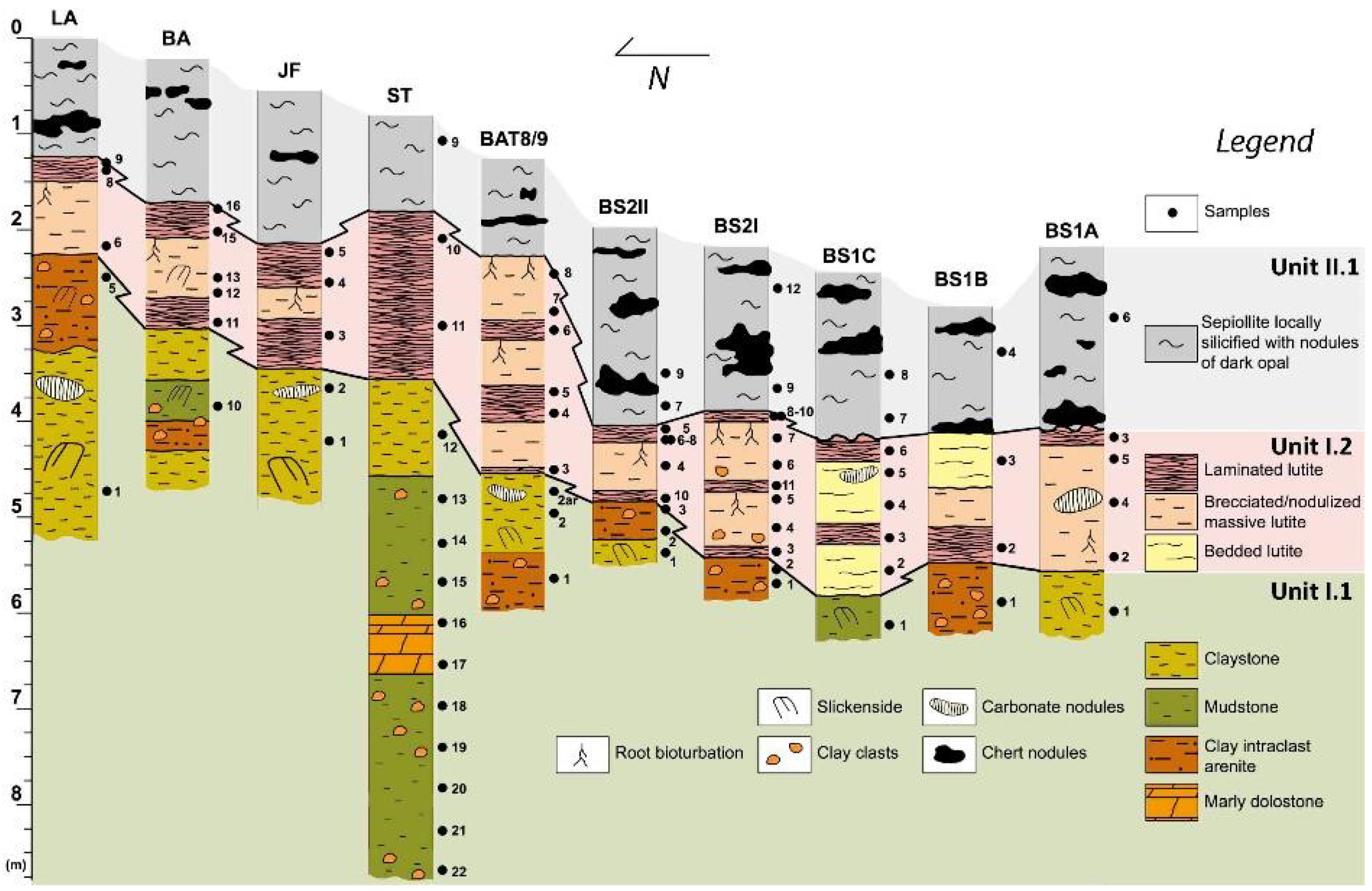
Figure 5.
Outcrop and hand-sample views of lithofacies: (a) lithofacies I.1-A composed of massive claystones with common slickensides; (b) close-up view of the boundary between I.2-A and I.2-B lithofacies; (c) hand-sample from lithofacies I.2-A showing conspicuous lamination and various colors; and (d) detail of opal-CT occurrences locally associated to Mg-clay lithofacies.

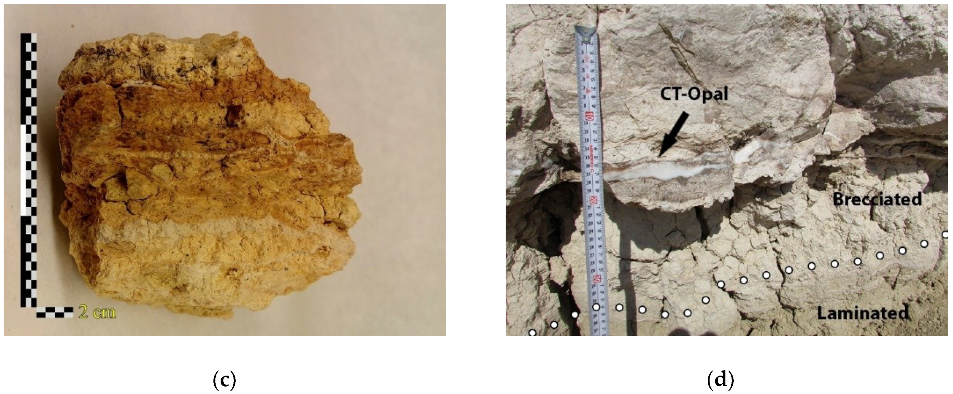
Figure 6.
(a) Laminar-turbulent microfabric of smectite (JF-01, lithofacies I.1-A) (SEM, SE); (b) calcite crystals (Ca) inserted between Mg-clay laminae (BAT8/9-2, lithofacies I.1-A); (c) K-feldspar (Fsp) grain showing a birrefringent fabric of skelsepic type (crossed polars) (BA-10, lithofacies I.1-B); (d) skeletal microfabric composed of smectite-rich intraclasts (BS2I-2, lithofacies I.1-C) (SEM, BSE); (e) laminar microfabric of sepiolite (BS2I-8, lithofacies I.2-A) (SEM, BSE); and (f) sepiolite bundles with fibers infilling porosities (sep) near crumpled smectite aggregates (sme) (ST-10, lithofacies I.2-A) (SEM, BSE).

Figure 7.
(a) Laminated lutite where alternating smectite (sme) and sepiolite (sep) laminae are shown. The transition from one to the other clay mineral in the same lamina is observed in the rectangle (0.3 mm width) (crossed polars and plane polarized light) (LAD-8, lithofacies I.2-A); (b) Laminar microfabric showing both thick (yellow points) and thin laminae (LAD-8, lithofacies I.2-A) (SEM, SE); (c) Hand sample showing alternating irregular banding where gel-like white sepiolite aggregates infill planar porosities (arrows) (BAT8/9-3, lithofacies I.2-A); (d) Hand sample showing grain-supported texture composed of sepiolite intraclasts (1), silty groundmass (2) and sepiolite cements (arrow) (BS2I-6, lithofacies I.2-B); (e) Nodular-brecciated sepiolite showing birefringent coatings (arrows) (BA-12, lithofacies. I.2-B) (crossed polars); (f) Laminar microfabric composed of interwoven sepiolite fibres (BS2I-7, lithofacies I.2-B) (SEM, BSE).
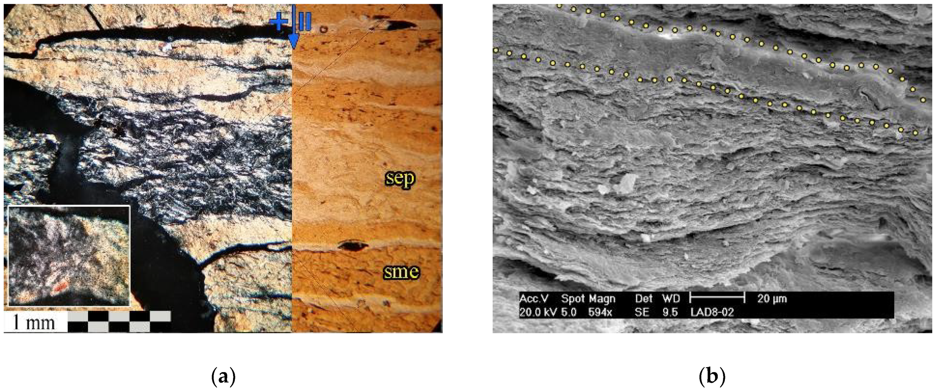

Figure 8.
(a) Laminar microfabric composed of sepiolite (BS2I-9, lithofacies II.1-A) (SEM, BSE); (b) sepiolite surface showing densely interwoven fibres (BS2I-9, lithofacies II.1-A) (SEM, BSE); (c) sub-angular morphologies (unknown composition and origin) infilling pores in sepiolite (arrows)and coated by fiber aggregates (BS2I-12, lithofacies II.1-A) (SEM, BSE); and (d) lepispheres of opal C-T (dotted) showing sepiolite fiber coatings. Scale of close-up image is 5 μm length (BS2I-9, lithofacies II.1-A) (SEM, BSE).


Figure 9.
(a) XRD patterns of selected clay fraction both oriented mounts (ethylene glycol) and randomly oriented showing the d (060) spacing; and (b) test of Christidis and Koutsopoulou [25] on representative smectite-rich sample (BS2II-1).
Figure 9.
(a) XRD patterns of selected clay fraction both oriented mounts (ethylene glycol) and randomly oriented showing the d (060) spacing; and (b) test of Christidis and Koutsopoulou [25] on representative smectite-rich sample (BS2II-1).

Figure 10.
XRD patterns showing variation in presence, intensity and shape of sepiolite reflections for the different units. The d-spacing values are in nm; numbers in bold are distinctive of high “crystallinity” sepiolite [17].
Figure 10.
XRD patterns showing variation in presence, intensity and shape of sepiolite reflections for the different units. The d-spacing values are in nm; numbers in bold are distinctive of high “crystallinity” sepiolite [17].
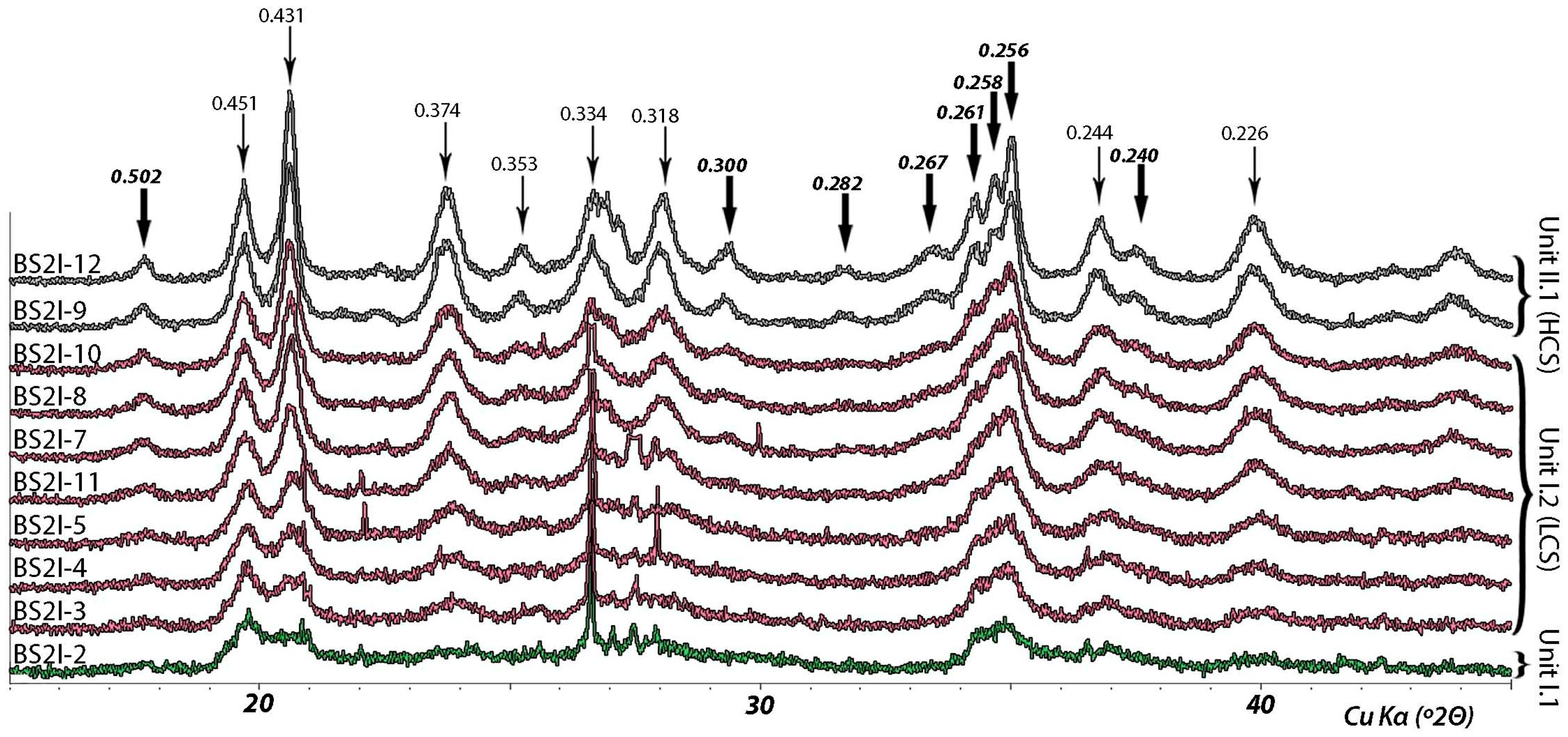
Figure 11.
Bivariate plot showing the distribution of sepiolite content vs sepiolite “crystallinity” (FWHM). The blue line separates low “crystallinity sepiolite” (LCS) from high “crystallinity” sepiolite (HCS).
Figure 11.
Bivariate plot showing the distribution of sepiolite content vs sepiolite “crystallinity” (FWHM). The blue line separates low “crystallinity sepiolite” (LCS) from high “crystallinity” sepiolite (HCS).
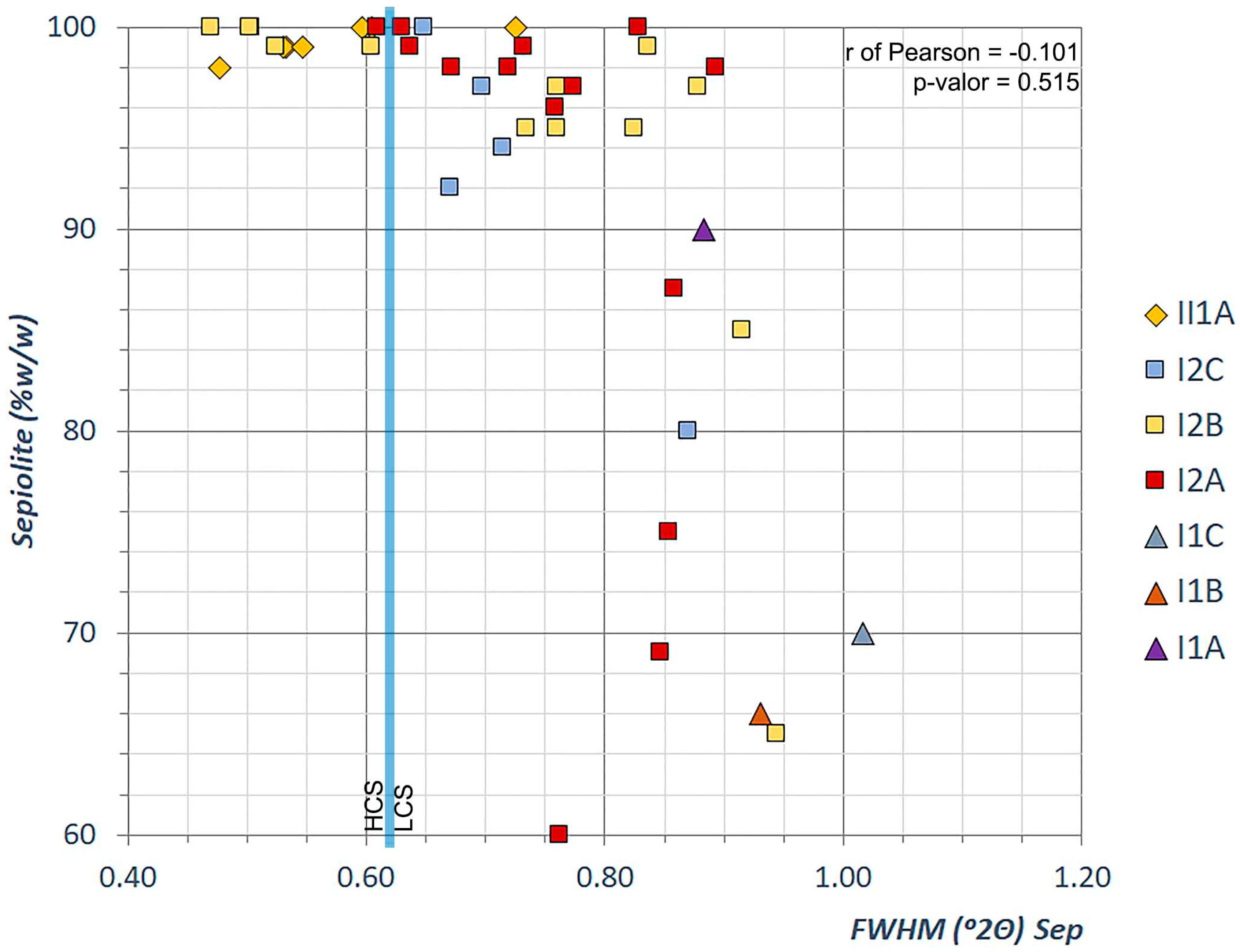
Figure 12.
(a) Lithostratigraphic log of BS2I showing the variation in the content of selected major elements; and (b) clay mineralogy and FWHM variation of sepiolite.
Figure 12.
(a) Lithostratigraphic log of BS2I showing the variation in the content of selected major elements; and (b) clay mineralogy and FWHM variation of sepiolite.
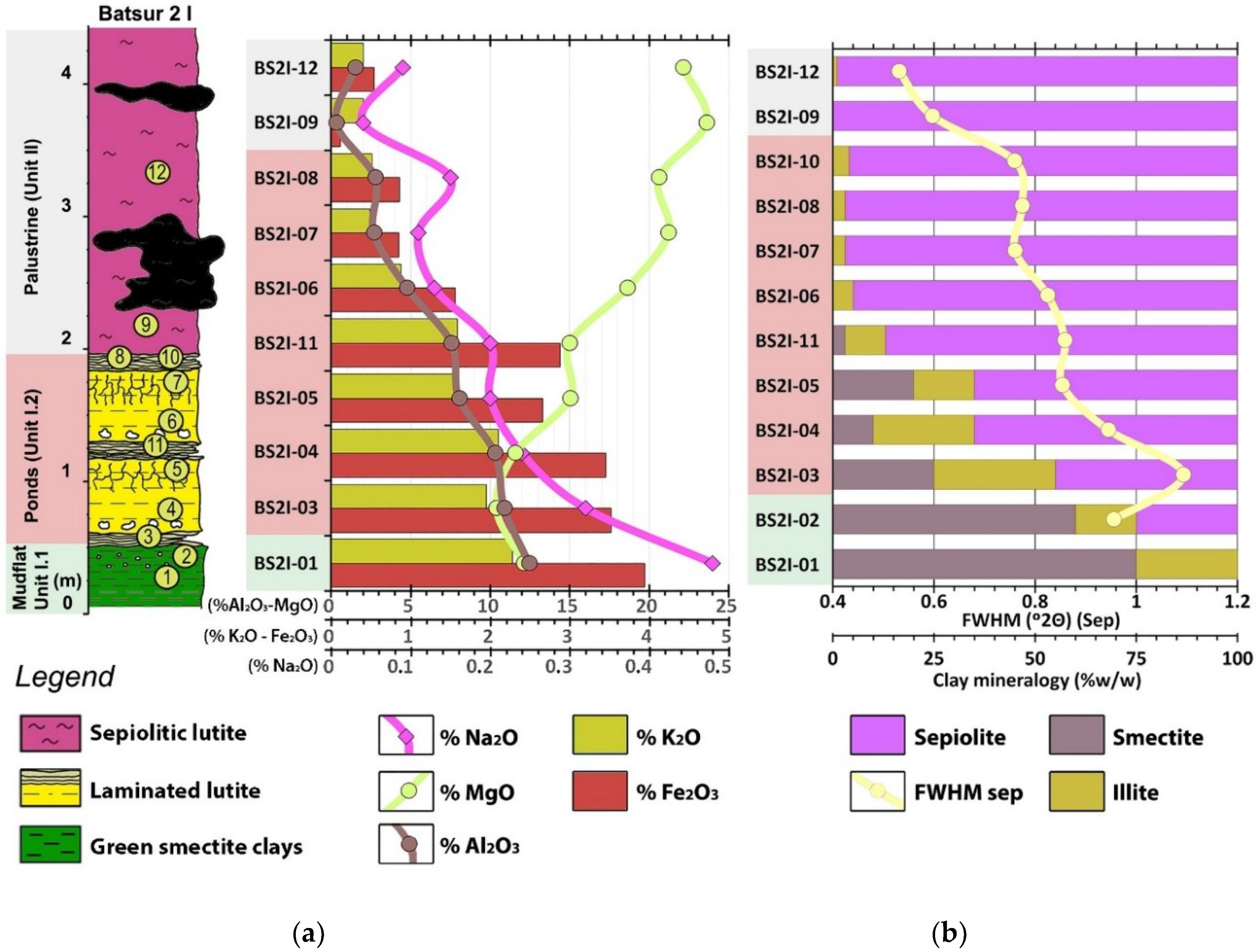
Figure 13.
Dendogram obtained from cluster analysis of major and trace elements. Four groups (G1 to G4) were differentiated.
Figure 13.
Dendogram obtained from cluster analysis of major and trace elements. Four groups (G1 to G4) were differentiated.
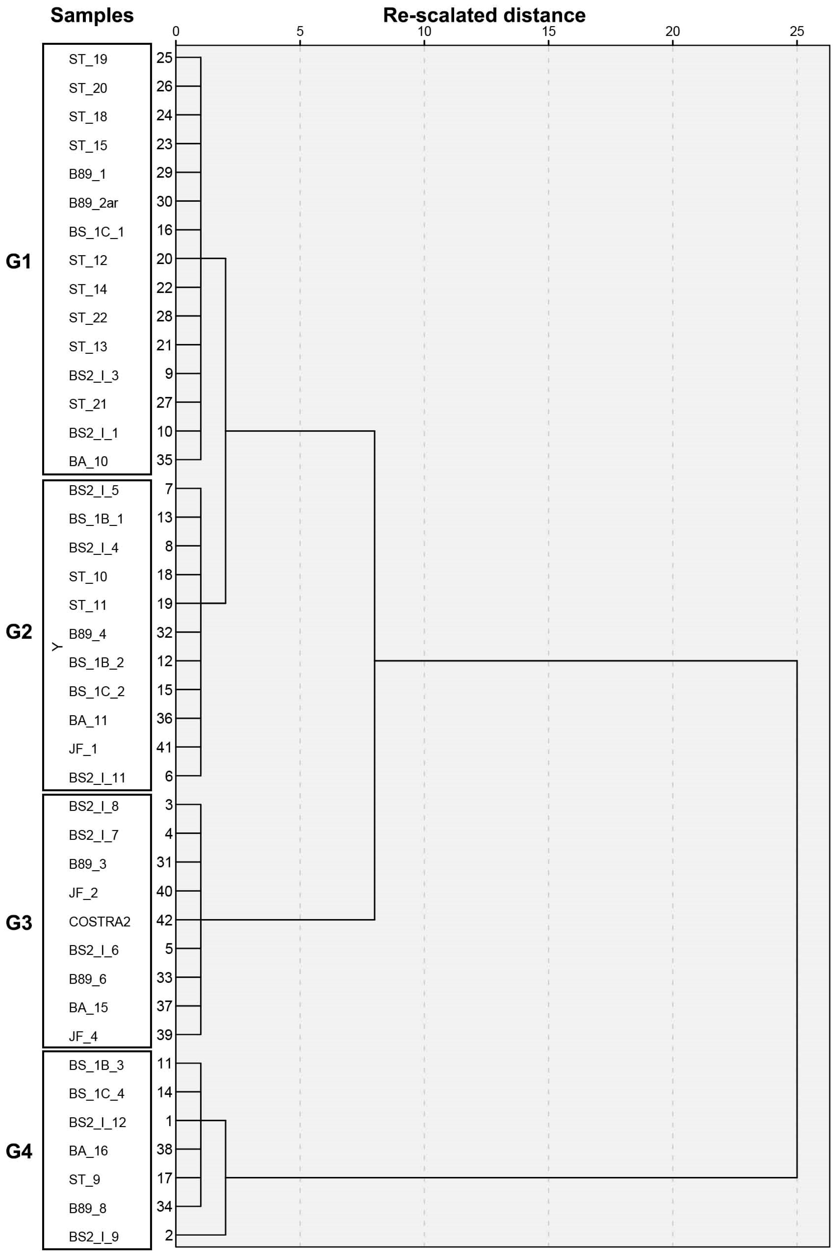
Figure 14.
Diagrams showing the maximum, minimum and mean (yellow line) values of selected major and trace elements from the different cluster groups. The compositional ranges of the elements according to their geochemical evolution give rise to 4 associations of elements: (a) Association of elements concentrated mainly in G1, represented by Ba and Ce; (b) Association of elements distributed from G1 to G4 that are separated into two overlapping groups represented by MgO and Al2O3; (c) Association of elements staggered from G1 to G4, represented by SiO2 and Fe2O3; (d) Association of elements that do not show defined trends, represented by Br and Cu.

Table 1.
Bulk (% w/w) and clay mineralogy (% w/w) of Unit I.1 lithofacies. Sepiolite FWHM values (°2Θ), crystallite sizes (Cr.) (nm) and “crystallinity” are also shown. Abbreviations are according to Whitney and Evans [27], except phyllosilicates (Phy), trace minerals (Tr) and not detected (-): Qz, quartz; Fsp, feldspar; Cal, calcite; Dol, dolomite; Sme, smectite; Sep, sepiolite; Ilt, illite; Kln, kaolinite. The order inside each lithofacies group of samples is related with the geographical location, from north to south, of lithological sections.
| Unit I.1 | Bulk Mineralogy | Clay Fraction | Sepiolite Features | ||||||||||
|---|---|---|---|---|---|---|---|---|---|---|---|---|---|
| Lf | Sample | Phy | Qz | Fsp | Cal | Dol | Sme | Sep | Ilt | Kln | FWHM | Cr. | Type |
| A | LA-1 * | 97 | 3 | Tr | - | - | 87 | - | 13 | - | |||
| A | JF-1 * | 100 | Tr | Tr | - | - | 6 | 82 | 12 | - | 0.809 | - | LCS |
| A | ST-12 | 98 | 2 | Tr | - | - | 98 | Tr | 2 | - | |||
| A | B8/9-2ar * | 100 | Tr | Tr | - | - | 91 | - | 9 | - | |||
| A | B8/9-2 * | 98 | 2 | - | Tr | - | 87 | - | 13 | - | |||
| A | BS2II-1 | 97 | 2 | 1 | - | - | 75 | - | 25 | - | |||
| A | BS1A-1 | 98 | 2 | Tr | - | - | - | 90 | 10 | - | 0.883 | 11 | LCS |
| B | BA-10 * | 76 | 17 | 7 | - | - | 78 | Tr | 22 | - | |||
| B | ST-13 | 95 | 5 | Tr | - | - | 95 | Tr | 5 | - | |||
| B | ST-14 | 96 | 4 | Tr | - | - | 84 | Tr | 16 | - | |||
| B | ST-15 | 98 | 2 | Tr | - | - | 85 | Tr | 15 | - | |||
| B | ST-18 | 90 | 2 | Tr | - | 8 | 77 | - | 19 | 4 | |||
| B | ST-19 | 92 | 2 | 6 | - | - | 73 | - | 20 | 7 | |||
| B | ST-20 | 89 | 4 | 7 | - | - | 83 | - | 15 | 2 | |||
| B | ST-21 | 91 | 5 | 4 | - | - | 80 | - | 20 | - | |||
| B | ST-22 | 97 | 2 | 1 | - | - | 83 | - | 17 | - | |||
| B | BS1C-1 | 89 | 3 | 4 | 4 | - | 12 | 66 | 22 | - | 0.931 | - | LCS |
| C | LA-5 * | 74 | 9 | 9 | 8 | - | 64 | - | 31 | 5 | |||
| C | B8/9-1 * | 96 | 2 | 2 | - | - | 100 | - | - | - | |||
| C | BS2II-3 | 96 | 3 | 1 | - | - | 70 | 10 | 20 | - | 0.645 | - | LCS |
| C | BS2II-2 | 98 | 1 | - | - | - | 75 | 5 | 20 | - | 0.800 | - | LCS |
| C | BS2I-2 | 97 | 2 | 1 | - | - | 60 | 25 | 15 | - | 0.956 | - | LCS |
| C | BS2I-1 | 97 | 2 | 1 | - | - | 75 | - | 25 | Tr | |||
| C | BS1B-1 | 98 | 2 | Tr | - | - | 10 | 70 | 20 | - | 1.017 | 6 | LCS |
| D | ST-16 | 67 | - | Tr | 1 | 31 | |||||||
| D | ST-17 | 30 | - | - | - | 70 | |||||||
* Previously reported by Pozo et al. [17].
Table 2.
Bulk (% w/w) and clay mineralogy (% w/w) of Unit I.2 lithofacies. Sepiolite FWHM values (°2Θ), crystallite sizes (Cr.) (nm) and “crystallinity” are also shown. Abbreviations are according to Whitney and Evans [27], except phyllosilicates (Phy), trace minerals (Tr) and not detected (-): Qz, quartz; Fsp, feldspar; Cal, calcite; Dol, dolomite; Sme, smectite; Sep, sepiolite; Ilt, illite; Kln, kaolinite. The order inside each lithofacies group of samples is related with the geographical location, from north to south.
| Unit I.2 | Bulk Mineralogy | Clay Fraction | Sepiolite Features | BET | ||||||||
|---|---|---|---|---|---|---|---|---|---|---|---|---|
| Lf. | Sample | Phy | Qz | Fsp | Cal | Sme | Sep | Ilt | FWHM | Cr. | Type | |
| A | LA-9 * | 100 | Tr | Tr | - | 13 | 78 | 9 | ||||
| A | LA-8 * | 100 | Tr | Tr | - | 23 | 64 | 13 | ||||
| A | BA-16 * | 95 | Tr | - | 5 | - | 100 | - | 0.609 | 15 | LCS | 328.0 |
| A | BA-15 * | 96 | 3 | 1 | - | |||||||
| A | BA-11 * | 99 | 1 | Tr | - | 11 | 83 | 6 | ||||
| A | JF-4 * | 100 | - | - | - | - | 100 | - | 0.630 | 14 | LCS | |
| A | JF-3 * | 100 | Tr | - | Tr | |||||||
| A | JF-2 * | 100 | Tr | - | - | |||||||
| A | COSTRA2 * | 100 | - | - | - | - | 100 | - | ||||
| A | ST-10 | 100 | Tr | Tr | - | 23 | 73 | 4 | LCS | |||
| A | ST-11 | 100 | Tr | Tr | - | 19 | 76 | 4 | LCS | |||
| A | B8/9-6 * | 95 | 5 | - | - | - | 100 | - | 0.829 | - | LCS | 360.0 |
| A | B8/9-5 * | 100 | Tr | - | - | - | 98 | 2 | 0.893 | - | LCS | 299.0 |
| A | B8/9-4 * | 95 | 3 | 2 | - | 7 | 88 | 5 | ||||
| A | B8/9-3 * | 100 | - | - | - | - | 98 | 2 | 0.719 | 12 | LCS | 355.0 |
| A | BS2II-5 | 98 | 1 | - | - | - | 99 | 1 | 0.638 | 13 | LCS | |
| A | BS2I-10 | 100 | - | - | - | - | 96 | 4 | 0.760 | 12 | LCS | |
| A | BS2I-8 | 98 | 2 | - | - | - | 97 | 3 | 0.774 | 11 | LCS | 352.4 |
| A | BS2I-11 | 98 | 1 | 1 | - | 2 | 87 | 10 | 0.859 | 8 | LCS | 305.7 |
| A | BS2I-11O | 18 | 65 | 17 | ||||||||
| A | BS2I-11C | - | 98 | 2 | ||||||||
| A | BS2I-5 | 95 | 2 | 2 | - | 5 | 75 | 20 | 0.854 | - | LCS | |
| A | BS2I-3 | 97 | 1 | 2 | - | 25 | 45 | 30 | 1.093 | - | LCS | |
| A | BS1C-6 | 90 | - | - | 10 | - | 98 | 2 | 0.672 | 15 | LCS | |
| A | BS1C-3 | 99 | 1 | - | - | 3 | 60 | 37 | 0.762 | 11 | LCS | |
| A | BS1B-2 | 95 | 3 | 2 | - | 1 | 69 | 30 | 0.847 | 9 | LCS | 323.5 |
| A | BS1A-3 | 99 | - | - | 1 | - | 99 | 1 | 0.733 | 13 | LCS | |
| B | LA-6 * | 72 | 8 | 7 | 13 | 8 | 85 | 7 | 0.915 | - | LCS | |
| B | BA-13 * | 100 | Tr | Tr | - | - | 95 | 5 | 0.760 | 12 | LCS | |
| B | BA-12 * | 100 | Tr | Tr | - | - | 97 | 3 | 0.878 | 10 | LCS | |
| B | B8/9-8 * | 100 | - | - | - | - | 99 | 1 | 0.525 | 17 | HCS | |
| B | B8/9-7 * | 100 | - | - | - | - | 100 | - | 0.504 | 18 | HCS | |
| B | BS2II-10 | 1 | 3 | - | 96 | |||||||
| B | BS2II-4 | 99 | Tr | Tr | - | - | 99 | 1 | 0.837 | 10 | LCS | 392.6 |
| B | BS2I-7 | 99 | 1 | - | - | - | 97 | 3 | 0.760 | 12 | LCS | 348.0 |
| B | BS2I-6 | 98 | 1 | 1 | - | Tr | 95 | 5 | 0.825 | 10 | LCS | 358.8 |
| B | BS2I-4 | 97 | 2 | 1 | - | 10 | 65 | 25 | 0.945 | - | LCS | 397.1 |
| B | BS1C-8 | 100 | - | - | - | - | 100 | Tr | 0.470 | 18 | HCS | |
| B | BS1C-7 | 100 | - | - | - | - | 100 | Tr | 0.503 | 17 | HCS | |
| B | BS1C-5 | 2 | - | - | 98 | - | 100 | Tr | 0.649 | 13 | LCS | |
| B | BS1A-5 | 100 | - | - | - | - | 99 | 1 | 0.605 | 14 | HCS | |
| B | BS1A-4 | 30 | - | - | 70 | - | 97 | 3 | 0.698 | 12 | LCS | |
| B | BS1A-2 | 100 | - | - | - | - | 95 | 5 | 0.735 | 13 | LCS | |
| C | BS1C-4 | 95 | - | - | 5 | - | 94 | 6 | 0.715 | 13 | LCS | 345.3 |
| C | BS1C-2 | 93 | 3 | 4 | - | 3 | 80 | 17 | 0.870 | 9 | LCS | |
| C | BS1B-3 | 99 | 1 | - | - | - | 92 | 8 | 0.670 | 13 | LCS | 213.9 |
* Samples previously reported by Pozo et al. [17].
Table 3.
Bulk (% w/w) and clay mineralogy (% w/w) of Unit II.1 lithofacies. Sepiolite FWHM values (°2Θ), crystallite sizes (Cr.) (nm) and “crystallinity” are also shown. Abbreviations are according to Whitney and Evans [27], except phyllosilicates (Phy), trace minerals (Tr) and not detected (-): Qz, quartz; Fsp, feldspar; Cal, calcite; Dol, dolomite; Sme, smectite; Sep, sepiolite; Ilt, illite; Kln, kaolinite. The order inside each lithofacies group of samples is related with the geographical location, from north to south, of lithological sections.
| Unit II.1 | Bulk min. | Clay Fract. | Sepiolite Features | BET | |||||
|---|---|---|---|---|---|---|---|---|---|
| Lf | Sample | Phy | Cal | Sep | Ilt | FWHM | Cr. | Type | |
| A | ST-9 | 100 | - | 100 | - | 0.726 | 13 | LCS | |
| A | BS2II-9 | 100 | - | 100 | Tr | 0.605 | 15 | HCS | |
| A | BS2II-7 | 100 | - | 99 | 1 | 0.533 | 17 | HCS | |
| A | BS2I-12 | 100 | - | 99 | 1 | 0.531 | 18 | HCS | |
| A | BS2I-9 | 100 | - | 100 | - | 0.597 | 16 | HCS | 371.08 |
| A | BS1B-4 | 100 | - | 98 | 2 | 0.477 | 18 | HCS | |
| A | BS1A-6 | 50 | 50 | 99 | 1 | 0.547 | 16 | HCS | |
© 2018 by the authors. Licensee MDPI, Basel, Switzerland. This article is an open access article distributed under the terms and conditions of the Creative Commons Attribution (CC BY) license (http://creativecommons.org/licenses/by/4.0/).
Share and Cite
MDPI and ACS Style
Herranz, J.E.; Pozo, M. Authigenic Mg-Clay Minerals Formation in Lake Margin Deposits (the Cerro de los Batallones, Madrid Basin, Spain). Minerals 2018, 8, 418. https://doi.org/10.3390/min8100418
AMA Style
Herranz JE, Pozo M. Authigenic Mg-Clay Minerals Formation in Lake Margin Deposits (the Cerro de los Batallones, Madrid Basin, Spain). Minerals. 2018; 8(10):418. https://doi.org/10.3390/min8100418
Chicago/Turabian StyleHerranz, Juan Emilio, and Manuel Pozo. 2018. "Authigenic Mg-Clay Minerals Formation in Lake Margin Deposits (the Cerro de los Batallones, Madrid Basin, Spain)" Minerals 8, no. 10: 418. https://doi.org/10.3390/min8100418
Note that from the first issue of 2016, this journal uses article numbers instead of page numbers. See further details here.