Economic Block Model Development for Mining Seafloor Massive Sulfides


Department of Geoscience and Petroleum, Norwegian University of Science and Technology, Sem Sælands vei 1, N-7491 Trondheim, Norway
*
Author to whom correspondence should be addressed.
Minerals 2018, 8(10), 468; https://doi.org/10.3390/min8100468
Submission received: 25 September 2018
/
Revised: 11 October 2018
/
Accepted: 16 October 2018
/
Published: 19 October 2018
(This article belongs to the Special Issue Deep-Sea Minerals and Gas Hydrates)
Abstract
:To support open-pit studies related to seafloor massive sulfides mining projects, an economic block-model is required. A modular framework is proposed to produce economic block models accommodating various levels of data. The framework is illustrated on a site of interest located on the Arctic Mid-Ocean Ridge. Random sampling based on literature datasets is performed to assign grades, porosity and grain density to the model. Other required parameters are produced using relationships found in the literature. Revenues are estimated using literature values within a net smelter return methodology. Mining costs are determined using the cost of a mining system and the estimated time required for excavating the ore. The excavating time is assessed through the specific energy for the ore and the mining machines. The specific energy is calculated with a hyperbaric rock-cutting model. An economic block value of each mining block is then provided. The mining block database resulting from the study constitutes a valuable input into further studies on resource development. The framework has also been used to support a sensitivity study. The availability of the marine assets has been found as having the greatest influence on the economic value of the study case.
1. Introduction
Since the 1960s, mining of deep-sea minerals has remained questionable [1]. A major part of current activities is related to exploration rather than exploitation. Resource assessments and technological solutions that can potentially enable deep-sea mining to become a reality are now required. The economic viability of deep-sea minerals depends on the in-situ value of the deposits and on the technological and cost challenges associated with the exploitation. Frameworks encompassing geological, geotechnical, technological and economic aspects are vital to support mineral resource and reserve assessments. Developing such frameworks is a challenging task due to scarce geological and geotechnical information. As per today, Nautilus Minerals is the only company worldwide who is committed to the commercial exploitation of Seafloor Massive Sulfides (SMS) deposits. Nautilus Minerals plans to start their offshore operations by the first half of 2019 [2]. The Japanese Ministry of Economy, Trade and Industry (METI) and the Japan Oil, Gas and Metals National Corporation (JOGMEC) just cleared the first SMS ore lifting from a 1600-m water depth [3]. SMS are also present on the Norwegian Continental Shelf (NCS) [4], and the present paper endeavors to present the first step in a resource assessment framework. The study case presented in this paper is an SMS mineralization located on the NCS; Loki’s Castle [5]. Within the paper, the term “deposit” will be used to qualify a mineralization and is not an indication of a classified resource. For cost estimations, the present study pre-supposes that the SMS deposit is exploited through open-pit mining. In the absence of drilling assays for Loki’s Castle, the presented methodology supports a conceptual study as defined in [6], which precedes the Pre-Feasibility Study (PFS) as defined in mining codes such as the NI 43-101 [7] or the JORC Code [8]. Open-pit studies are generally performed in two steps, first finding the Ultimate Pit Limit (UPL) and then solving a scheduling problem such as the Capacitated Final Open Pit (CFOP) or the Capacitated Dynamic Open Pit (CDOP) [9,10,11]. The UPL problem is generally solved using the graph-based Lerchs–Grossmann Algorithm (LGA), first presented by Lerchs and Grossmann [12], or by using the flow network method presented by Picard [13]. Both methods require the ore body to be reduced to a block model where each mining block is attributed an economic net value. Establishing a block model for a land deposit is a well-defined task, which is supported by extended geological knowledge and a fair return of experience when it comes to cost estimation. To the contrary, knowledge of SMS deposits is limited. From a geological perspective, important parameters, such as grade distributions, geotechnical parameters and deposits geometries, are uncertain. To alleviate those uncertainties for the Loki’s Castle deposit, information from other SMS deposits including the well-explored Trans-Atlantic Geotraverse (TAG) orebody [14] will be transposed directly onto a tentative geometry of the orebody. These parameters are fundamental for the calculation of revenues and costs.
The present paper proposes a framework for the calculation of mining blocks’ economical value. A strong focus is put on calculation methodologies and on the establishment of the framework. The data presented in this paper are used to illustrate the framework and its potential. Thus, the results presented in the paper do not aim at representing the actual value of Loki’s Castle. The theory relevant for revenue and cost estimations will be reviewed to lay the foundations of the framework. Further, the methodology forming the backbone of the framework will be presented with a particular focus on cost estimation. For each mining block, the developed methodology: (1) simulates geological parameters; and (2) calculates the specific energy required during excavation in order to (3) estimate the specific energy-dependent costs and, eventually, the economic value. The materials and data used as inputs for the framework such as geological and economic parameters will then be presented. As part of the results, the outputs from the framework will be presented by evaluating the potential economic in situ value of the case study. Further, a sensitivity analysis for parameters related to the mining system will (1) display the capabilities of the established framework as a supporting tool for preliminary feasibility studies and (2) identify the relative importance of a mining system’s parameters on the economic value. Limits of the framework and future research topics will be addressed as part of the discussion.
2. Background
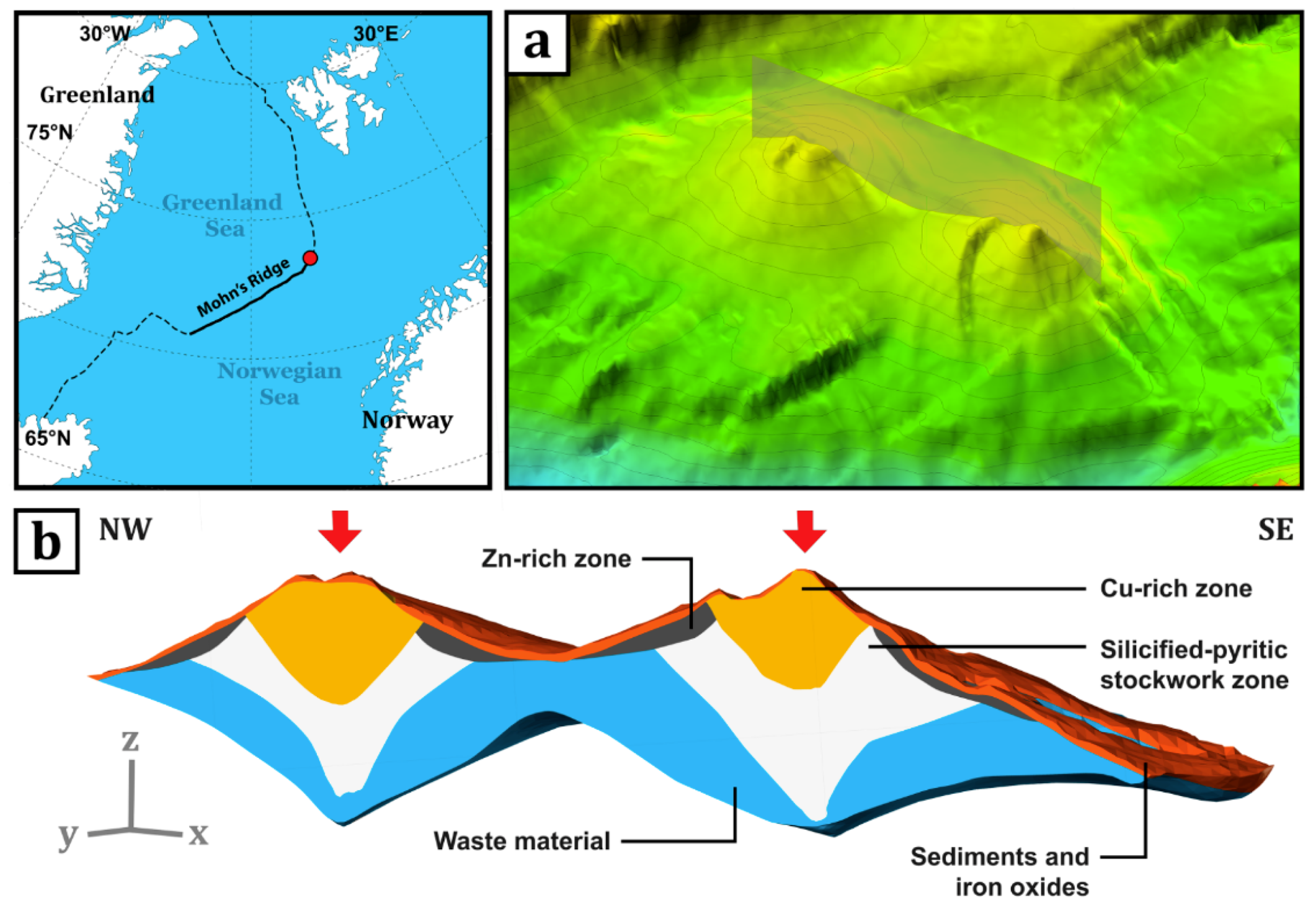
The Loki’s Castle ore deposit, located at about a 2400-m depth within the Mohn-Knipovich ridge transition (ca. 73°30′ N), represents a typical basalt-hosted black-smoker type vent site that has been observed with seafloor dimensions (ca. 140–160 m in diameter) directly comparable to those of the TAG active hydrothermal mound at the Mid-Atlantic Ridge (26°08.2′ N; [14,15]). Based on multi-beam data collected during the MarMine Cruise in 2016 [16], a 3D model of the Loki’s Castle deposit has been created using LeapFrog Geo® (4.2.3, Leapfrog, Emeryville, CA, USA). No drilling data are available for Loki’s Castle, but for the context of this study, a simplified geological model has been setup using the TAG deposit geometry as an analogue. Following the suggested characterization of the TAG by Hannington et al. [17], six geological domains are represented, among which three are considered as potential ore domains (see Figure 1). Table 1 gathers the main features of Loki’s Castle 3D model, which will be used for applying the methodology presented in the paper. Note that the Si-rich zone mainly corresponds to the sub-seafloor stockwork mineralization as described by Hannington et al. [17]. The stockwork is represented by pyrite-silica breccias and an intensely silicified wall rock, where sulfide minerals are disseminated in the deeper levels of the deposit. It is desirable to quantify minerals of the stockwork with more observable characteristics (sampling) than presented in Hannington et al. (1998) because lower grade bulk-tonnage styles of mineralization can be expected (see Section 5.2). In this study, however, the Si-rich zone represents a hypothetical case of an economic orebody. The deposit is defined here by the combined volume of the three geological domains, which will be attributed revenues (Cu-rich, Zn-rich and Si-rich).
3. Theory
In order to determine the economic value of a mining block, , one needs to determine both the revenues generated by selling the valuable material present in the block, , and the mining costs, , related to the extraction and processing of the ore present in the mining block, b [18]:
3.1. Revenues
The revenues generated by selling the valuable minerals present in a mining block can be estimated using the concept of Net Smelter Return (NSR) as described in [19] (Section 7 therein). The revenues calculation using the NSR is based on the tonnage of valuable elements present in the mining block, , a percentage net smelter return representing the loss of value during smelting activities, NF, the recovery in the beneficiation plant, , and the price of commodities, . A portion of the elements present in a mining block will be lost during mining and is represented by the recovery factors . Considering the selling price of an element, the mining block revenues can be expressed as:
can be calculated using the concentration of the element of interest, generally expressed as a grade, , the bulk density of the mining block, and the volume of the mining block :
When is not readily available from the drilling data, can be determined using the grain density, , and the porosity, , according to the formula [20] (Section 9 therein):
3.2. Costs
For the purpose of open-pit studies, the mining cost of a mining block, b, results only from the operational costs (OPEX) related to the extraction, transport (logistics) and processing of the ore present in the block [18]. In a deep-sea mining setup, the cost of extraction comes from the use of marine assets (vessels, machines, personnel) required for extracting a given block. The mining cost, , related to the production of a mining block can be expressed using the following relationship:
If the marine assets used to extract the block are composed of a vessel (including a vertical transportation system) and mining machines, then:
Currently, the details of profitable mining setups are not proven especially within the Norwegian environment. For example, it has not been determined yet whether the produced ore would be offloaded offshore into transport barges (ship-to-ship transfer) or if the mining vessel would stop its mining activity and offload the produced ore via port-call. It is hereby proposed to gather both and into an equivalent . Further, it is likely that an offshore mining setup will encounter interruption during production due to adverse weather conditions, breakdowns, planned maintenance and possibly crew-changes. Aligned with common practices in the maritime industry, it is assumed that non-producing offshore assets still cost money even though no revenue is generated. In order to account for non-production duration that reduces the overall production, a unitless asset availability factor, is used:
The mining cost of a block, b, is now expressed:
where:
and:
is the duration required for the offshore assets to produce the ore present in the mining block, . The rate-per-day convention will be used because vessel costs are generally expressed that way in the marine industry [21]; Nautilus Minerals also uses the daily rate convention to express the OPEX related to the production support vessel [22] (Table 20-10 therein).
3.3. Mining Time and Specific Energy
3.3.1. Mining Time
The mining time, (in h), is defined by the ratio between the mining block volume, (in m3), and the rate of excavation, (in m3/h):
The specific energy, , is commonly used within the mining industry to calculate rates of progression or excavation rates [23] (Section 7.1 therein). The specific energy is defined by the following relationship:
where:
- is the specific energy (in kWh/m3 or MPa)
- is the available cutting power (in kW), i.e., the portion of the machine total power dedicated to the cutting machinery
- is the achieved excavation rate (in m3/h)
Combining Equations (11) and (12):
is an input given by the mining system characteristics, and is determined by the resolution of the block grid. determination is discussed within the next paragraph.
3.3.2. Specific Energy
The excavation of rock in the hyperbaric environment is different from surface mechanical excavation because additional forces can appear during the cutting process as a result of cavitation in the failure area; the rock will tend to change its behavior from brittle to ductile [24]. Hyperbaric forces appear as well during the dredging process of sand and by extension should be taken into consideration for the excavation of sediments [25]. Nautilus Minerals also used for predicting the rate of production, but used an averaged value for for their studies of the Solwara 1 deposit [22] (Section 19.7.7 therein). Nautilus Minerals’ prediction is based on a proprietary model developed together with SMD [26] and the University of Delft. It is proposed to calculate following the method described by Miedema [27] (Section 9 therein). This method has been selected for computational considerations. Other discrete element-based methods have been considered too time consuming and resource demanding, as each block would require a separate study for itself (examples of such studies in [28,29,30]). In addition, Miedema’s model gives results similar to hyperbaric rock cutting experiments [24] and has been used for the preliminary design of trenching equipment [31]. Using Miedema’s convention, the can be expressed as a function of the horizontal cutting forces, , the depth of cut trench, , and the width of the blade, :
The magnitude of is determined as a function of:
- The cutting parameters: w, , the blade angle, , and the friction angle between the blade and the rock, ;
- The rock parameters: the cohesive strength of the rock, , and the internal friction angle of the rock, .
- The hyperbaric forces function of the environmental pressure (calculated using the ambient pressure at the work site, , and the level of cavitation ).
- To summarize:
The actual calculation process of is outside the scope of this paper, and the authors refer to Miedema’s proposed methodology [27] (Section 9 therein).
can be determined using the method described by Detournay and Atkinson [32], introducing the Péclet number, . is calculated using the cutting speed, , the cut trench height, , the porosity of the rock, , the viscosity of the pore fluid, , the compressibility of the pore fluid, , and the intrinsic permeability of the rock, :
is determined following the value obtained for :
- , no cavitation occurs, ,
- , cavitation partially occurs,
- full cavitation is established,
4. Methodology
4.1. Description of the Proposed Framework
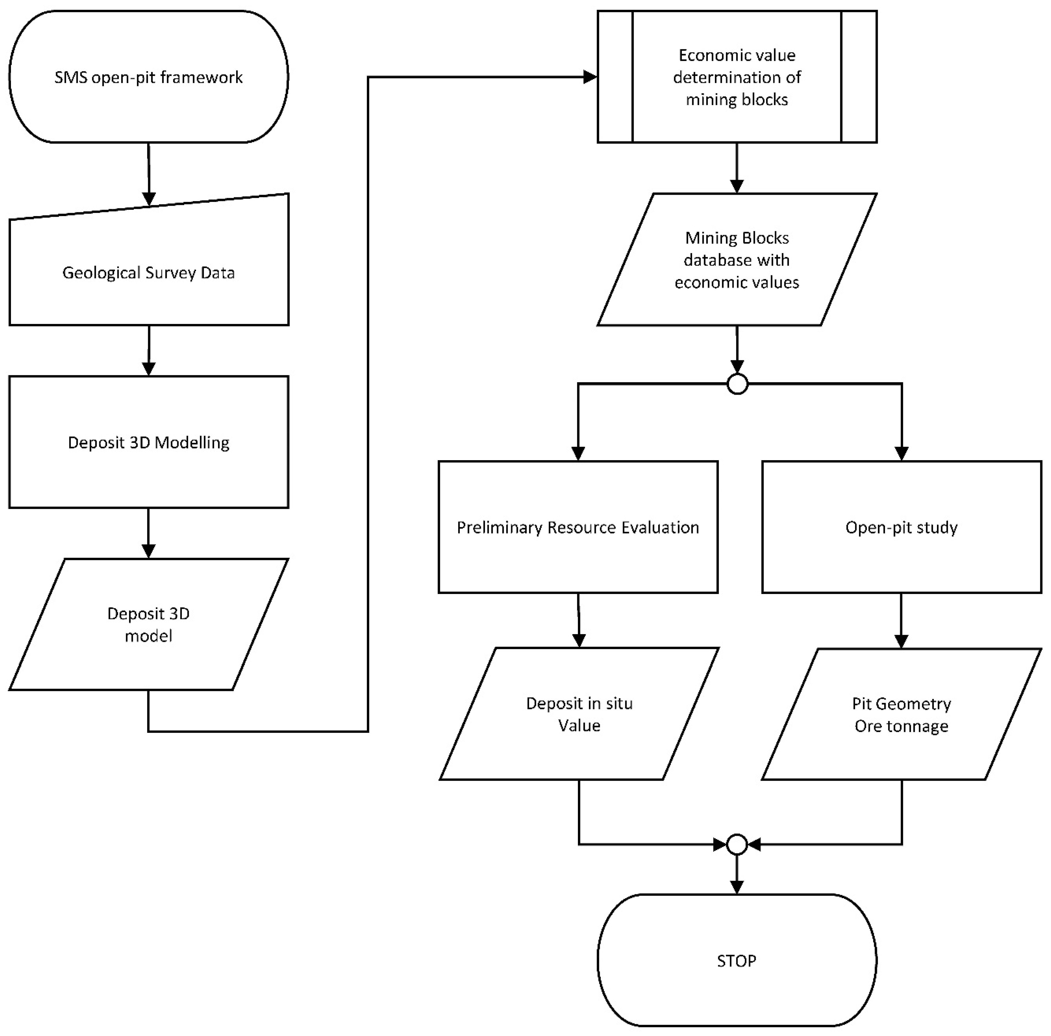
The framework proposed within this paper is currently supported by Leapfrog Geo® (4.2.3, Leapfrog, Emeryville, CA, USA) for the deposit’s 3D modelling and visualization; and MATLAB® (R2017a, The MathWorks, Natick, MA, USA) for the grades and geotechnical simulations followed by the economic value calculation. The output of the framework is a database that can be used either by an open-pit study support software, such as Datamine (STUDIO RM Version 2.3, Datamine, Denver, CO, USA); or to assist with preliminary resource assessments. A visual representation of the framework is shown in Figure 2.
4.2. Determination of the Block Model Parameters
Because no drilling assays are available for our study case deposit, a probabilistic approach is considered for simulating the grades and the geotechnical parameters required in the block-model. When data are available for a deposit or an analogous deposit, cumulative distribution functions (CDFs) are established using the statistical parameters of available datasets (e.g., mean and standard deviation). When datasets are unavailable for a given parameter:
- -
- either the parameter will be calculated using known relationships with one or several of the previously simulated parameters,
- -
- or arbitrarily attributed using a typical value from the literature.
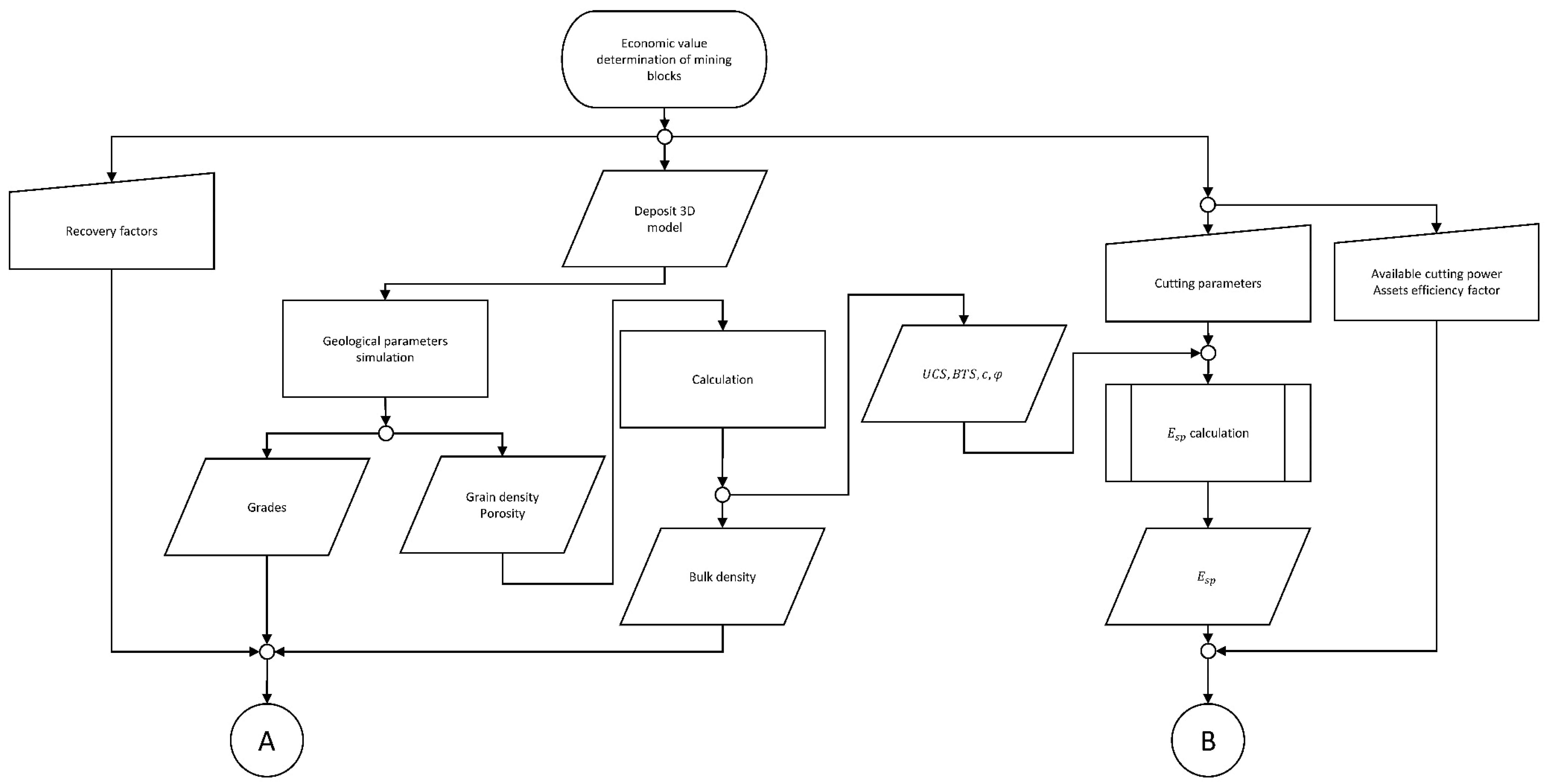
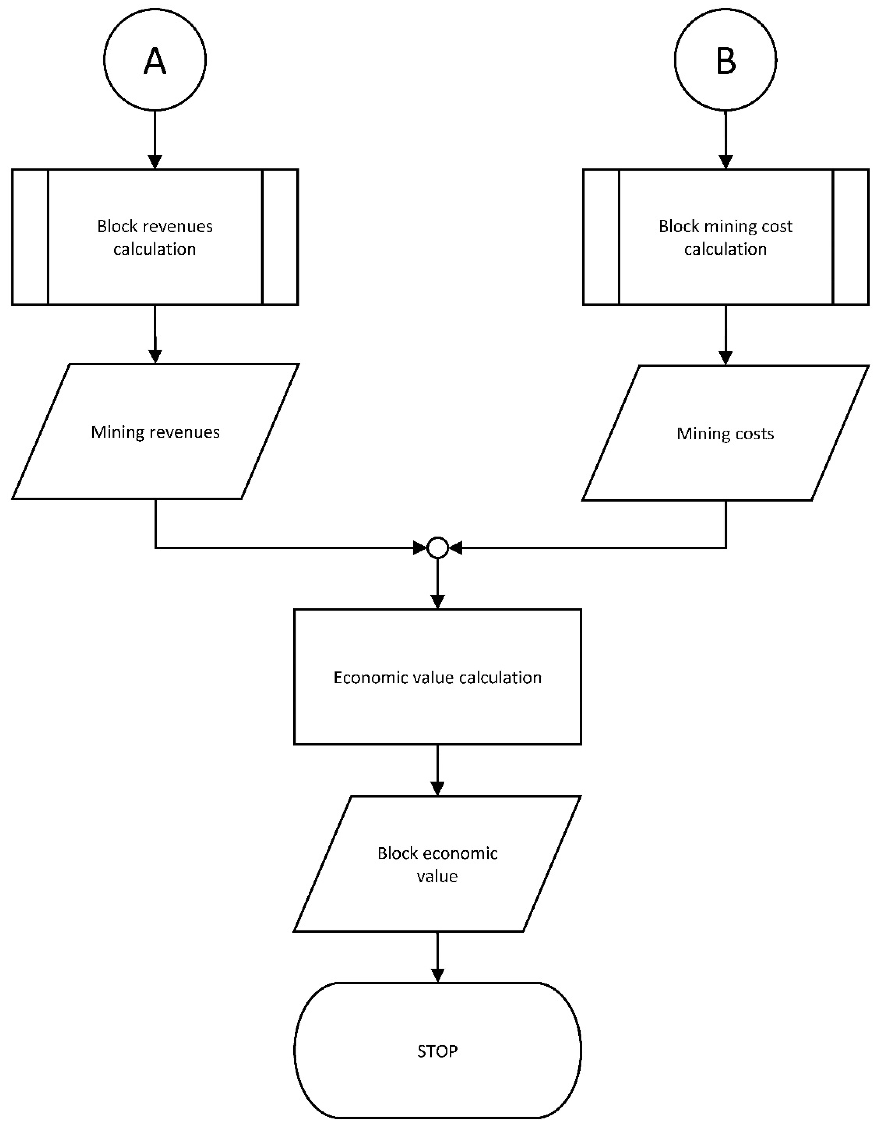
A summary of the methodology used for developing the Loki’s Castle block-model is given in Appendix A as a flowchart (Figure A1 and Figure A2).
4.2.1. Grades
For each mining block of the ore-domains, the grades of Cu, Zn, Au and Ag are sampled using the MATLAB (R2017a) random number generator on Cumulative Density Functions (CDFs) (see Section 5.2). Other domains such as waste or sediments are not attributed any grades, i.e., they have no revenues. Even though sediments can present grades in interesting amounts, the lack of data drove this decision. This has no impact on the illustration of our methodology, but future studies should consider adding revenues to sediments. The reader will also find that a maximum value has been attributed to each element in each ore domain. Any simulated value above the reported maximum value has been replaced by the mean. As an example, considering a dataset with a mean value of 0.7 wt% Cu and a maximum value of 8 wt% Cu, any simulated value above 8 wt% will be replaced by 0.7 wt%. The results produced using this procedure will show a mean lower than the mean of the original data.
4.2.2. Porosity, Grain Density, Bulk Density and Permeability
The same method as the one presented in Section 4.2.1 is used to attribute porosity, , and grain density, (see Section 5.3). Same as for the grades, extremely high values have been truncated using pre-defined maximum values. The bulk density, , is calculated based on already simulated values for and . The permeability, , is calculated based on (see Section 5.4).
4.2.3. Pore Fluid Dynamic Viscosity, Compressibility and Local Pressure
The dynamic viscosity of the pore fluid, , and compressibility, , are fixed values found in the literature (see Section 5.6). The local pressure, , is fixed according to values reported during investigations [16].
4.2.4. Cohesive Strength and Internal Friction Angle
When no data are available for the cohesive strength, , and internal friction angle, , the literature gives an alternative method to determine and based on known Unconfined Compressive Strength, , and Brazilian Tensile Strength, [27] (p. 246, 247, 250):
This method can produce abnormally high values for (. Abnormally high values are subsequently truncated and arbitrary allocated a value of , if the calculated value is superior to . UCS and BTS are calculated based on (see Section 5.5).
4.2.5. Metal Prices, Payable Metal Contents and Cost of Assets
Metal prices, payable metal contents and cost of assets per day are fixed values found in the literature (see Section 5.1).
4.3. Determination of Specific Energy
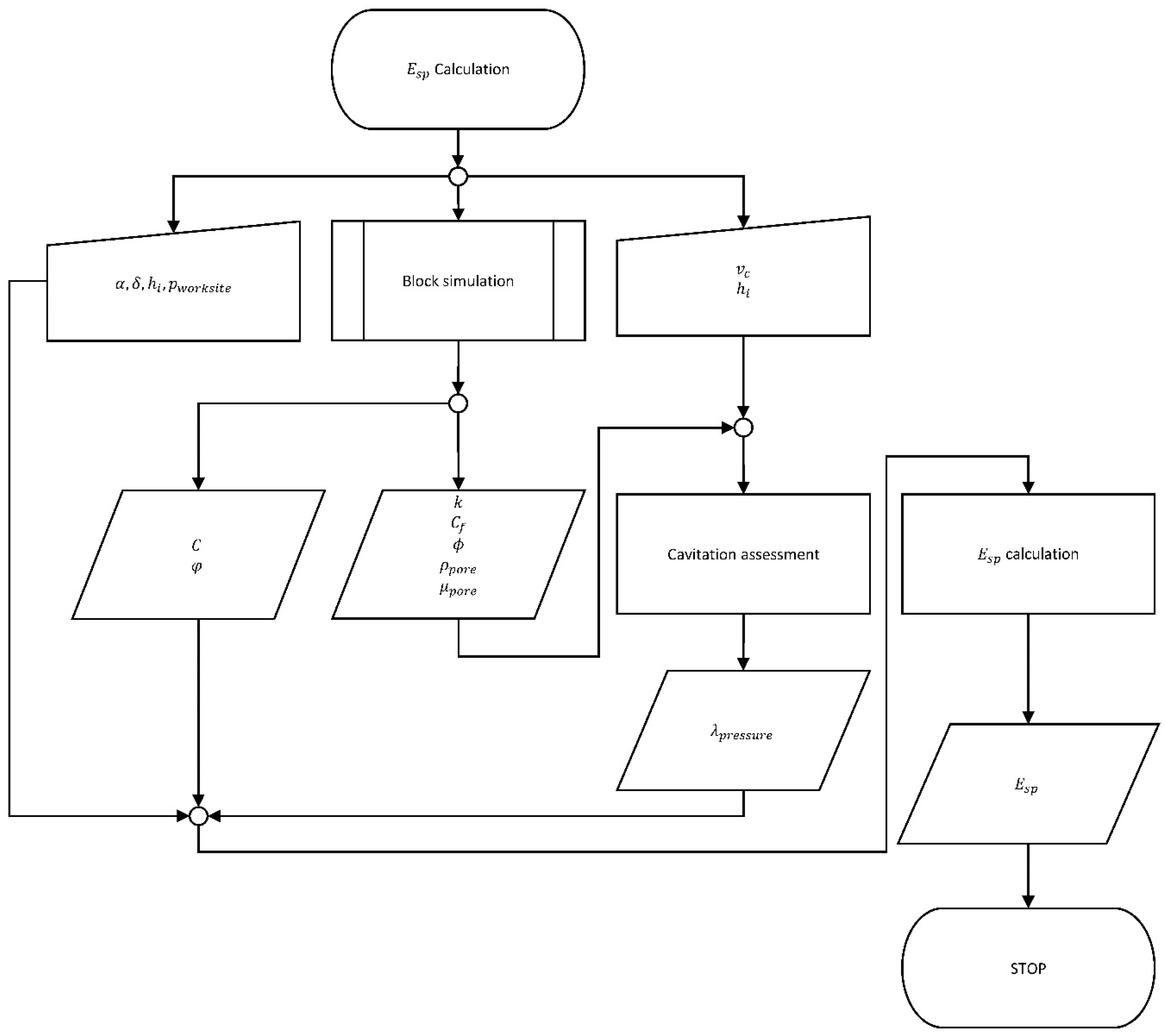
For each mining block, is determined using a set of MATLAB routines based on Miedema’s proposed methodology (see Section 3.3.2) and the geotechnical parameters produced during the previous steps (Appendix A; see Figure A1 for a visual summary of the geotechnical parameters’ production). A visual summary of the calculation sub-framework is given in Figure 3.
4.4. Sensitivity Study
A sensitivity study will be performed on a selection of parameters pertaining to the mining system. For each considered parameter, an evaluation of the deposit’s economic value (measured as the in situ dollar value) will be presented while keeping the other parameters fixed. Following the individual sensitivity study, a multi-parameter study will be performed in order to determine the relative influence of each parameter. The multi-parameter study will be executed by successively estimating the economic value of the deposit while varying the parameters between extreme values. Extreme values represent high and low scenarios. The high and low scenarios are designed to investigate the influence of the parameters within a 25% deviation from the base value. As an example, if the base value for is 2 MW, the low scenario considers a value for of 1.5 MW, and the high scenario considers a value of of 2.5 MW. The results of the multi-parameter study will be gathered in a tornado chart to determine visually the parameters of main importance.
5. Materials and Data
5.1. Fixed Parameters
5.1.1. Cutting Parameters
Specific energy is calculated using several independent parameters linked to the actual mining equipment setup. A sensitivity analysis will be performed for and . Other parameters are kept fixed using typical values found in the literature (e.g., [27]). The list of fixed parameters for cutting is given in Table 2.
5.1.2. Mining Costs
5.1.3. Commodity Prices
Commodity prices used for this paper have been determined by averaging the commodity values over the last five years and are presented in Table 4.
5.1.4. Mining Recovery Rate
The study presented in this paper assumes that the loss of material between excavation and processing is negligible, and, thus
5.1.5. Net Smelter Return
5.2. Grades
Using the assays presented by Hannington et al. [17], CDFs have been constructed for each element based on lognormal distributions. The lognormal distribution parameters for each element in each ore domain are summarized in Table 6. The maximum values have been set following the observed maximum value from the CDFs’ populations found in the literature [17].
5.3. Porosity and Grain Density
5.4. Permeability
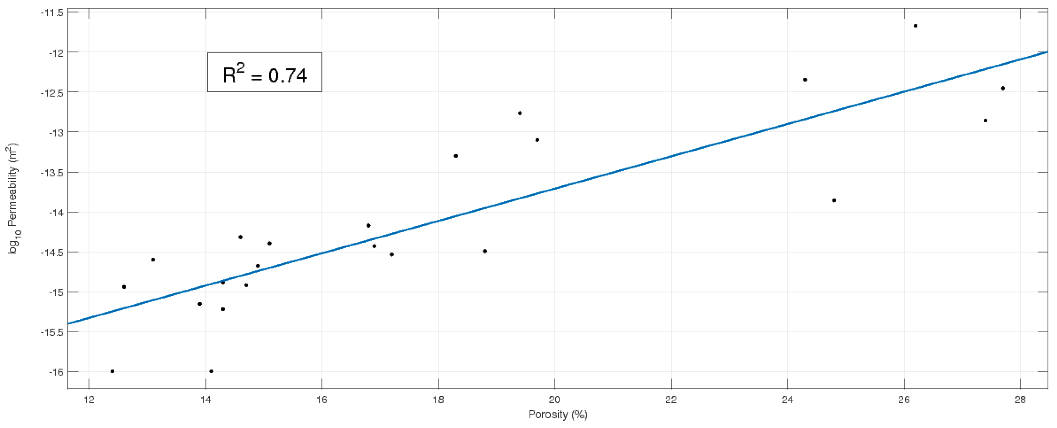
Little information is available regarding the permeability of SMS deposits. Available information related to the permeability of drill-core samples was taken from the Mothra hydrothermal vent field located on the Endeavour segment of the Juan de Fuca Ridge (North West America, Pacific Ocean) [38]. In addition, Zhu et al. [38] found a relation between porosity and permeability and distinguished two different populations in their dataset. Using the values given in their article, a relationship is found for the global dataset population while conserving a satisfactory correlation factor, as shown in Figure 4.
In order to calculate the permeability, , of a block based on the previously simulated porosity, , the following relationship is used (based on the regression shown in Figure 4):
5.5. UCS and BTS
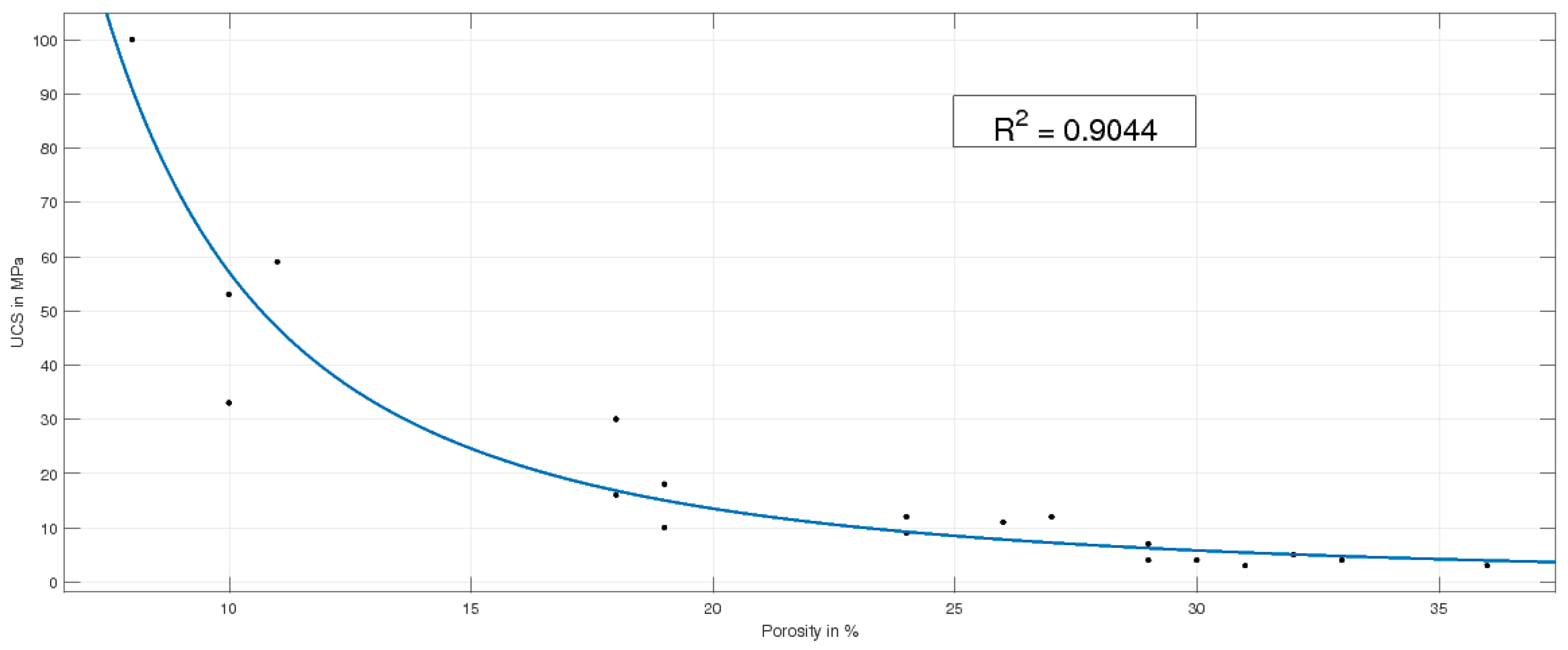
Some relationship has been found between the UCS and BTS values and the porosity of some SMS samples [39,40]. Waquet and Fouquet [39] gave relationships between UCS and the porosity of SMS, but the samples used were deeper in the orebody than the one used by Yamazaki and Park [40] (chimney material only). No explicit formulation of the relation between UCS and is given by Waquet and Fouquet [39], and an exponential regression has been reproduced based on the value given in the paper, as shown in Figure 5.
Due to the lack of information on the UCS value when , this relationship produces abnormally high values at low porosity values. Consequently, high values are truncated and set to 100 MPa (the maximum value found in the dataset used to produce the relationship).
The BTS/porosity relationship was only given by Yamazaki and Park [40], and the following relationship will be used:
5.6. Pore Fluid Dynamic Viscosity and Compressibility, Local Pressure
Dynamic viscosity, , and compressibility, , are needed for the prediction of cavitation and are related to the fluid encountered by the blade during the mining process, i.e., the pore fluid. The pore fluid encountered will be either seawater or a mixture of seawater and hydrothermal fluid. No information could be found regarding the dynamic viscosity and the compressibility of the hydrothermal fluids. Consequently, the study presented here assumes that pore fluids are similar to high salinity water (as pore fluids present a high density due to the elevated concentration of metallic ions). As and are both affected by temperature, it is assumed that pore fluids encountered by the mining machine are at a temperature equivalent to the seabed temperature (the seabed temperature was observed between and during the MarMine cruise [16]). Ambient pressure at Loki’s Castle is about . Nayar et al. [41] gave some values for seawater’s and at various pressures, temperatures and salinities. Values of interest are reproduced in Table 9 and Table 10.
In the frame of a conservative study, the value maximizing in the condition closest to this paper’s study case should be used. For this paper, the following values will be used:
- ,
- .
Future sensitivity studies will benefit from varying the value of and .
5.7. Processing Costs
It is assumed that if an SMS deposit is relatively small, the generated revenues cannot cover the investment needed for a dedicated process plant. An option is to sell the extracted material to an existing mine, which will process the extracted material further. The buyer’s processing cost can be transferred to the economic value of a mining block. A potential buyer for the material excavated at Loki’s Castle deposit could be the future mine related to the development of the Nussir deposit [42]. The processing costs presented in Nussir deposit’s scoping study have been reproduced in Table 11. Nussir deposit’s processing costs have been compared to values generated by the InfoMine cost model [43].
Nussir deposit’s processing costs are lower than InfoMine costs as only Cu is concentrated from the ore within the scoping study. InfoMine costs are provided for the concentration of three products. For the case study, it is intended to concentrate on four products for the study case; thus, InfoMine figures will be used. In order to account for (1) possible extra costs resulting from SMS having a different mineral composition than conventional ore such as, e.g., Volcanic Massive Sulfides (VMS), and (2) the cost related to additional processing steps, it was decided to consider a maximum value of 24.34 USD/t for processing costs in the sensitivity analysis. This represents a 25% increase of the highest value provided by InfoMine.
These costs differ from what can be extrapolated from [44]. In the Japanese model, processing costs (referred to as “ore dressing” in [44]) are based on a specific mining system where ore separation starts on the seabed followed by leaching on land in order to sell a concentrate to a smelter. According to the data given in [44], for a production rate of 4080 t/d, 308 days per year over 15 years, the processing costs are in the range of 4.8 $/t. However, due to the leaching process and local conditions, the Japanese model introduced waste disposal costs reaching 175 $/t. Due to its specificity, the Japanese cost model will not be used in this paper.
6. Results
6.1. Grades and Tonnages
Ten simulations have been performed as part of our study case. In order to illustrate some typical early information needed for defining tentative mining methods and perform early economical assessment, some results are gathered in Table 12.
6.2. Economic Sensitivity Analysis and Relation to Specific Energy
An economic sensitivity analysis has been performed on one realization of the deposit (35,076 blocks). A summary of the simulated and calculated geotechnical parameters used for the sensitivity analysis is presented in Table 13.
6.2.1. Specific Energy and Cut Trench Height
The specific energy has been calculated using the fixed cutting parameters defined in Section 5.1.1, while varying the depth of the cut trench, . The results for the specific energy calculations are given in Table 14. Related mining time has been calculated for = 1 MW and = 1.
The sensitivity study performed on shows the impact of this cutting parameter selection on the mining time necessary for the exploitation of the deposit. The extreme values of total mining time given in Table 14 were combined with a realization of grades and considering = 19.47 $/t, in order to show the influence of on the economic value of the deposit as presented in Table 15.
- A reduced mining time for the excavation of the deposit from 596 days to 439 days; this is a 26% reduction of the total mining time; and
- An increased economic value of the deposit from approximately −69.6 M$ to approximately −32.5 M$, equivalent to an approximate 53% decrease of the deficit economic value of the deposit.
6.2.2. Assets’ Availability Factor
The influence of has been investigated using the most efficient value for the cut trench depth, m while maintaining and = 19.47 $/t. The results are presented in Table 16.
It can be seen from Table 16 that decreasing from one to 0.5 decreases the economic value of the deposit from approximately −32.5 M$ to approximately −136.6 M$, i.e., an approximate 320% decrease of the economic value of the deposit.
6.2.3. Available Cutting Power
The influence of has been investigated using the most efficient values for m, and = 19.47 $/t. The results are presented in Table 17.
Increasing from 1 MW to 3 MW resulted in increasing the economic value of the deposit from approximately −32.5 M$ to approximately 36.9 M$, i.e., an approximate 214% increase of the economic value of the deposit.
6.2.4. Processing Costs
The influence of has been investigated using the most efficient values for m, and = 3 MW. The results are presented in Table 18.
Increasing from 14.60 $/t to 24.34 $/t resulted in decreasing the economic value of the deposit from approximately 41.6 M$ to approximately 32.2 M$, i.e., an approximate 23% decrease of the economic value of the deposit.
6.2.5. Multi-Parameter Sensitivity Study
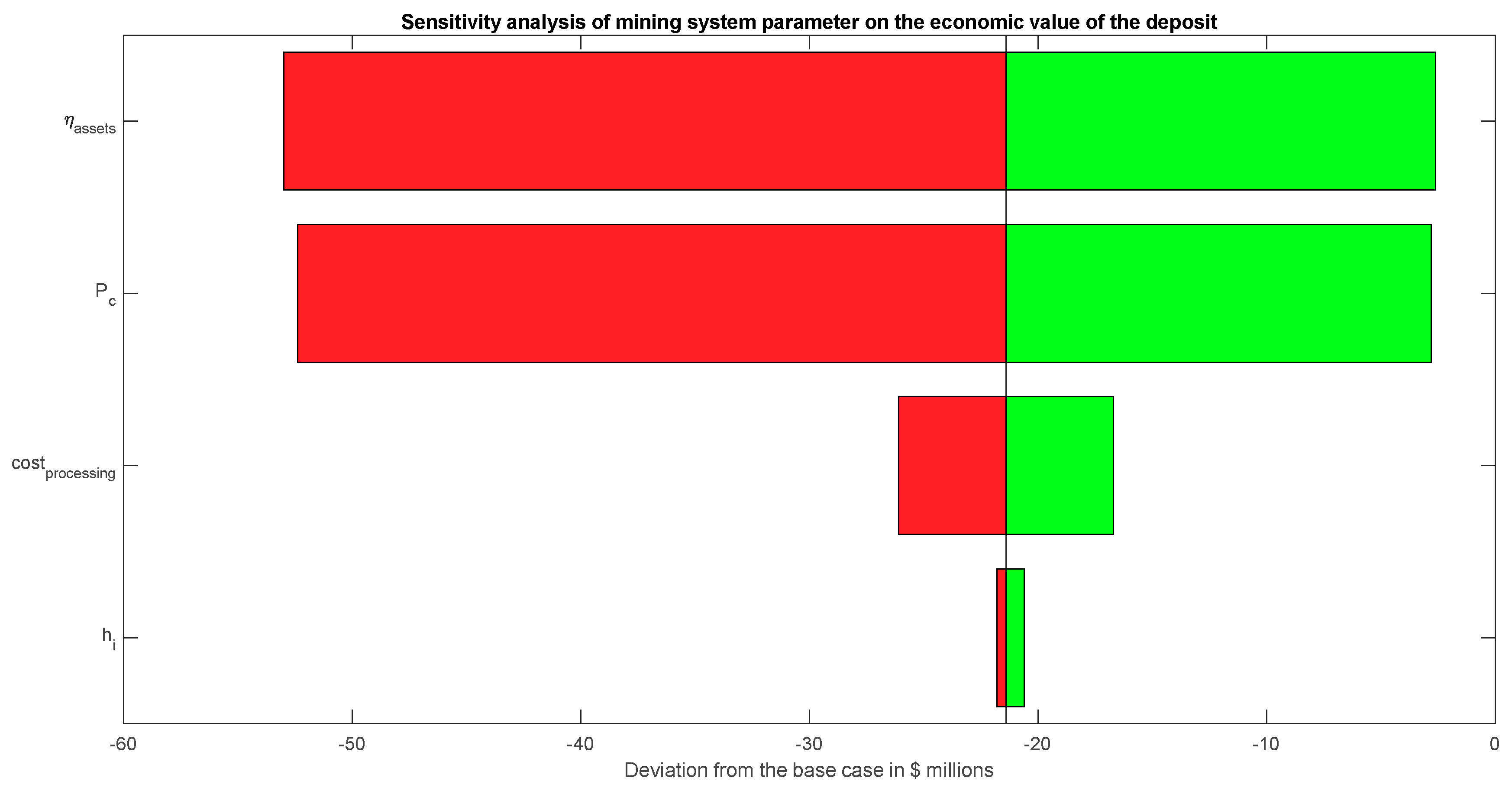
A multi-parameter sensitivity analysis was performed in order to determine which parameter was the most influential on the predicted economic in situ value of the deposit. Considered parameters are , , and . Table 19 summarizes the value of the parameters for the base case, high and low scenarios.
Table 20 presents the results obtained for the base case and the high and low scenarios.
A visual representation of the results is presented in Figure 6. It is observed that is the parameter of highest influence on the deposit economic value. shows a similar importance as .
7. Discussion
7.1. Geological Uncertainties
The calculation of the cohesive strength, c, and the internal friction angle, φ, presents a two-fold uncertainty. The first uncertainty originates from the actual relationship used for calculating c and φ using the UCS and the BTS (see Section 4.2.4). The second uncertainty originates from the values calculated for the UCS and BTS using simulated values for ϕ (see Section 5.5). Concerning the first uncertainty, the relationship used for calculating c and φ produced abnormally high values for φ, which led to the decision of truncating those values to a predetermined maximum. In addition, there is no certitude that the rock present in the target deposit will follow the same relationship between c, φ, UCS and BTS. Concerning the second uncertainty, the values used for calculating the UCS and BTS values based on the porosity, ϕ, originate from different geological settings: there is no assurance that the target deposit’s UCS and BTS will follow the same relationship. In addition, the relationship used to calculate UCS and BTS has been obtained from a dataset where few or no samples were available for ϕ < 10% (for UCS, see Figure 5; for BTS, reference is made to [40] (Figure 7 therein). Reminding that the simulated average value of ϕ for the target deposit is 4.17% (see Table 13), it is necessary to question the validity of the used relationship between UCS, BTS and ϕ.
The same remarks are relevant for the calculation of the permeability, k, where the dataset used for regression does not show any sample with ϕ < 10% (see Figure 4).
The framework’s calculation pipeline for c, φ and k will require updates when more geotechnical knowledge is acquired, especially for the deeper sections of the deposit where lower values of ϕ are expected. When drilling cores are available, the calculation pipeline for c and φ will be replaced by direct sampling onto distributions produced by tri-axial testing results. Similarly, the calculation pipeline for k will be replaced by direct sampling onto distributions produced by permeability tests on actual rock samples.
7.2. Specific Energy
The specific energy, , is the basis on which mining costs are evaluated (see Section 3.2 and Section 3.3), and its evaluation strongly depends on the produced values of c, φ and k. Therefore, the uncertainties surrounding the evaluation of c, φ and k (see Section 7.1) are directly transferrable to the evaluation of and further cascaded to the evaluation of the mining costs and economic value of the mining blocks. The values of obtained using Miedema’s model are most valid when the cutting process is performed with a straight blade and the cutting velocity is perpendicular to the blade [27] (Section 9.6 therein). Such conditions are not likely to be met, and other blade shapes and cutting head arrangements can be considered (e.g., [22] (Figure 19-34 therein)), though no available models exist for evaluating their . Such hyperbaric cutting head studies may find inspiration in [45,46], though these models have been developed for surface application and lack hyperbaric forces. A sensitivity study has been performed on the deposit when changing the depth of penetration of the cutting blade, . The mining time required for excavating the mineralized domain varies between 439 days and 596 days considering and (see Table 14). The observed variation is directly linked to the occurrence of full or partial cavitation as part of the hyperbaric cutting forces’ calculation process (respectively an average for = 0.1 m and an average for = 0.01 m). Even though the method used for the calculation of the hyperbaric rock cutting forces does not encompass all the complexity of the actual hyperbaric rock cutting process, the observed mining time variation indicates the importance of machine control. The impact of machine control on the rate of excavation (and thus, the economic value of a mining block) should be studied further and updates on hyperbaric rock cutting model integrated for future revision of the framework.
7.3. Assets Availability Factor
The assets’ availability factor, , has been assessed as the most influential factor on the economic value of the target deposit (see Figure 6). Further studies of will be crucial for deposit evaluation exercises. Establishing is a task involving several parameters including weather operability, maintenance requirements and logistics.
The weather operability, or “workability”, of a single equipment or operation is itself a complex topic, which may require the creation of a dedicated framework for its resolution [47]. An example of guidance for establishing weather operability criteria was proposed by DNV-GL in [48]. This guidance is a common standard within the marine industry and is used as a base for comparison of advanced techniques [49,50]. As described in the guidance, establishing the weather operability for an equipment or an operation includes the knowledge of the sequence of operations, failure mode and contingency scenarios [48] (Section 4 therein). In addition, the guidance introduces a reducing factor, the alpha-factor, which will reduce the weather operability because of the uncertainty of weather forecasts combined with operation durations [48] (B700 therein). Weather-induced delays and weather dependency can be modelled using discrete event simulation techniques [51,52].
Maintenance requirements will influence by making equipment unavailable for production during maintenance activities in order to comply with the maintenance objectives [53,54]. Finding the optimal maintenance policy that will optimize will require finding the right policy by adjusting the Corrective Maintenance (CM) and Preventive Maintenance (PM) policies in order to maximize the “limiting efficiency” of the mining system [55]. The study of maintenance policies can be performed using a discrete event simulation approach [56,57,58].
Logistics requirements will influence by introducing downtimes related to refueling of the offshore assets, ore transport and personal work rotations. Finding the key levers of logistics in order to maximize can be solved using discrete event simulation techniques [59,60,61,62,63].
It is believed that each project would require a dedicated study of in order to account for the local environmental conditions and mining system setup and that a discrete-event simulation approach would be adequate [64].
7.4. Available Cutting Power
The available cutting power has been found as the second most influential parameter in the sensitivity analysis. The framework presented in the paper assumes that a single cutting machine is used for excavation. Another assumption is that excavation is the limiting production factor, i.e., the ore is recovered to the surface as fast as it is excavated. The combination of excavation and ore lifting can be further analyzed using discrete-event simulation techniques as described in Section 7.3. From an available cutting power perspective, taking the Nautilus Minerals mining setup as an example [22], two machines are used for excavating the seabed material (the auxiliary miner and the bulk miner [22] (Section 19.5.3 therein). In the event of several machines collaborating in the excavation activities, an approach to integrate their respective contribution would be to use an equivalent available cutting power, . would replace Pc in Equation (12). could be approached as a function of (1) the available cutting power of each machine, , and (2) an efficiency factor for the excavation setup, . The efficiency factor, , reflects the potential downtime resulting from interactions between the excavating machines, which is equivalent to reducing . The following formula could be used:
In an ideal situation, excavating machines would work independently of each other and = 1. As discussed for in Section 7.2, could be estimated using discrete event simulation techniques.
7.5. Process Route
The framework presented in the paper assumes that the excavated ore will be sold directly to a processing plant for further treatment. Lacking information about the ore characteristics relevant for designing a process route, using the NSR seemed the best option. For other processing routes such as leaching, other cost structures could be used as presented by Yamazaki et al. [44]. For a given project, when the process flowchart is available, the processing cost and revenue pipelines will have to be reviewed. In that event, revenues will be updated by using new values for NF and in Equation (2). Similarly, processing costs will be updated by either a new value for in Equation (9).
7.6. Capabilities of the Framework
The framework has shown its usefulness for supporting single- and multi-parameter sensitivity studies. The results presented in the paper are not representative of the actual value of the case study and cannot be used for reporting resources or reserves. A future sequence of feasibility studies can be supported by the framework by replacing the data used in the paper by drill hole data and then quantifying resources and reserves as per relevant codes’ requirements [6,7,8]. Due to its modularity, the framework allows for studying the introduction of new data or new models. The framework can be improved further when deep-sea mining knowledge increases in order to refine the obtained results.
8. Conclusions
A methodology to develop an economic block model for SMS deposits has been presented. The framework integrates both geotechnical and economical parameters of SMS deposits allowing for sensitivity studies and preliminary economic evaluation. Challenges such as scarce geological data (grades, tonnages and geotechnical parameters) and cost evaluation (mining, processing and refining) have been addressed. Even though the lack of actual samples from the target deposit Loki’s Castle has been overcome by using data from analogue deposits, drill hole data will be essential for improving the framework’s parameters. The framework introduces a mixed economic structure sharing characteristics from land mining activities (e.g., net smelter return to estimate mining revenues) and a marine excavation model (i.e., hyperbaric rock cutting model to estimate mining costs). The framework has been used to support a multi-parameter sensitivity analysis of the economic value of the target deposit. The availability of marine assets has been found to have the greatest influence on the economic value of the target deposit, increasing the in-situ value of the deposit from −$52.4 m to −$2.8 m when increasing the availability of marine assets from 0.56 to 0.94. The validity of the data used to produce the results has been challenged, and the framework can be updated in the future as the knowledge of SMS deposits’ geology and deep-sea mining systems technology increases. The framework can already be used to support open-pit studies and preliminary economic assessments.
Author Contributions
All authors participated in the conceptualization activities. M.L. created the piece of software supporting the framework (MATLAB and Excel) and produced the formal analysis, methodology and visualization. C.J. and S.L.E. reviewed and edited the original draft. S.L.E. produced the original 3D model of Loki’s Castle.
Funding
This research was funded by the Norwegian Research Council (Norske Forskningsråd, NFR) and associated project industrial partners grant No. 247626/030 and through the Strategic Research Areas 2014–2023—NTNU Oceans. The APC was funded by the Norwegian Research Council (Norske Forskningsråd, NFR) grant No. 247626/030.
Conflicts of Interest
The authors declare no conflict of interest. The funders had no role in the design of the study; in the collection, analyses or interpretation of data; in the writing of the manuscript; nor in the decision to publish the results.
Appendix A. Block Model Development Methodology, Flowchart
Figure A1.
Loki’s Castle block-model development methodology, Part 1 of 2.

Figure A2.
Loki’s Castle block-model development methodology, Part 2 of 2.

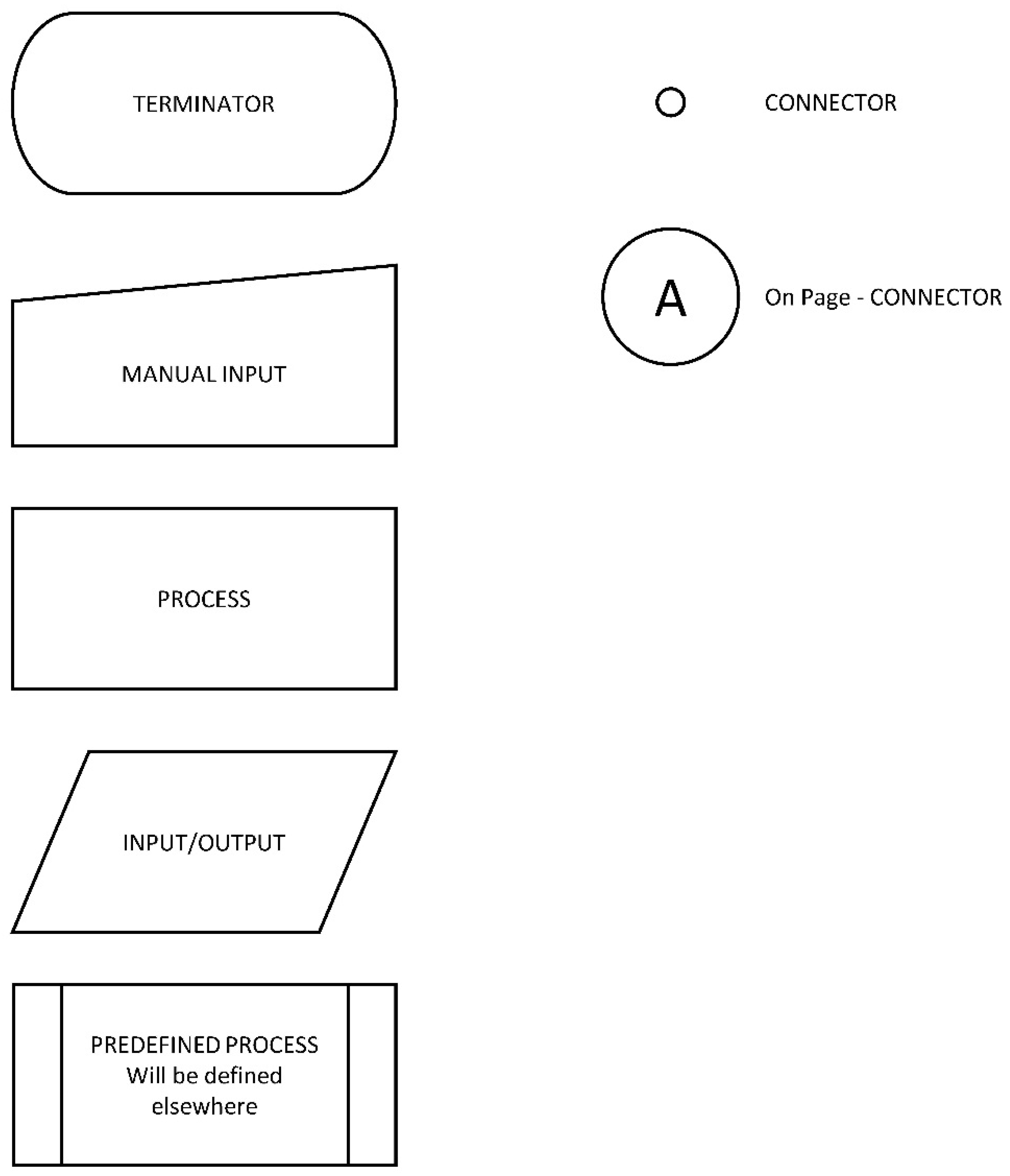
Appendix B. Flowcharts’ Legend
Figure A3.
Legend for flowcharts.

References
- Mero, J.L. The Mineral Resources of the Sea, 1st ed.; Oceanography Series; Elsevier: Amsterdam, The Netherlands; London, UK; New York, NY, USA, 1965; Volume 1, ISBN 978-0-08-087037-3. [Google Scholar]
- Nautilus Minerals Press Release Number 2017-21. Available online: http://www.nautilusminerals.com/irm/PDF/1930_0/Nautilusprovidesprojectupdate (accessed on 21 December 2017).
- METI; JOGMEC World’s First Success in Continuous Ore Lifting Test for Seafloor Polymetallic Sulphides. Available online: http://www.meti.go.jp/english/press/2017/0926_004.html (accessed on 21 December 2017).
- Brekke, H. Seabed Search for Metals Surging Ahead. Available online: http://www.npd.no/en/Publications/Norwegian-Continental-Shelf/No-1-2017/Minerals/ (accessed on 21 December 2017).
- Pedersen, R.B.; Rapp, H.T.; Thorseth, I.H.; Lilley, M.D.; Barriga, F.J.A.S.; Baumberger, T.; Flesland, K.; Fonseca, R.; Früh-Green, G.L.; Jorgensen, S.L. Discovery of a black smoker vent field and vent fauna at the Arctic Mid-Ocean Ridge. Nat. Commun. 2010, 1, 126. [Google Scholar] [CrossRef] [PubMed] [Green Version]
- Runge Picock Minarko. Minimum Engineering Study Requirements. Available online: https://www.rpmglobal.com/wp-content/uploads/mp/files/resources/files/rpm-perspectives-2015-128.pdf (accessed on 10 October 2017).
- CIM NI 43-101 Standards of Disclosure for Mineral Projects 2011. Available online: http://web.cim.org/standards/documents/block484_doc111.pdf (accessed on 10 October 2017).
- AusIMM, T. M. I. JORC Code, 2012 Edition 2012. Available online: http://www.jorc.org/docs/JORC_code_2012.pdf (accessed on 10 October 2017).
- Alvarez, F.; Amaya, J.; Griewank, A.; Strogies, N. A continuous framework for open pit mine planning. Math. Methods Oper. Res. 2011, 73, 29–54. [Google Scholar] [CrossRef]
- Caccetta, L. Application of optimisation techniques in open pit mining. In Handbook of Operations Research in Natural Resources; Springer: Boston, MA, USA, 2007; pp. 547–559. ISBN 978-0-387-71815-6. [Google Scholar]
- Caccetta, L.; Hill, S.P. An Application of Branch and Cut to Open Pit Mine Scheduling. J. Glob. Optim. 2003, 27, 349–365. [Google Scholar] [CrossRef]
- Lerchs, H.; Grossmann, I.F. Optimum Design of Open-Pit Mines. In Transactions CIM; Canadian Institute of Mining and Metallurgy: Montreal, QC, Canada, 1965; Volume 58, pp. 17–24. [Google Scholar]
- Picard, J.-C. Maximal Closure of a Graph and Applications to Combinatorial Problems. Manag. Sci. 1976, 22, 1268–1272. [Google Scholar] [CrossRef]
- Rona, P.A.; Klinkhammer, G.; Nelsen, T.A.; Trefry, J.H.; Elderfield, H. Black smokers, massive sulphides and vent biota at the Mid-Atlantic Ridge. Nature 1986, 321, 33. [Google Scholar] [CrossRef]
- Humphris, S.E.; Kleinrock, M.C. Detailed morphology of the TAG Active Hydrothermal Mound: Insights into its formation and growth. Geophys. Res. Lett. 1996, 23, 3443–3446. [Google Scholar] [CrossRef]
- Ludvigsen, M.; Aasly, K.; Ellefmo, S.L.; Hilário, A.; Ramirez-Llodra, E.; Søreide, F.X.; Falcon-Suarez, I.; Juliani, C.J.; Kieswetter, A.; Lim, A.; et al. MarMine Cruise Report—Arctic Mid-Ocean Ridge 15.08.2016–05.09.2016. 2016. Available online: https://brage.bibsys.no/xmlui/handle/11250/2427715 (accessed on 10 October 2017).
- Hannington, M.D.; Galley, A.G.; Herzig, P.M.; Petersen, S. 28. Comparison of the TAG mound and stockwork complex with Cyprus-type massive sulfide deposits. In Proceedings of the Ocean Drilling Program, Scientific Results; Texas A & M University: College Station, TX, USA, 1998; Volume 158, pp. 389–415. [Google Scholar] [CrossRef]
- Hustrulid, W.A.; Kuchta, M.; Martin, R.K. Open Pit Mine Planning and Design, 3rd ed.; CRC Press: Boca Raton, FL, USA, 2013; Volume 1, ISBN 978-1-4822-2117-6. [Google Scholar]
- Wellmer, F.-W.; Dalheimer, M.; Wagner, M. Economic Evaluations in Exploration, 2nd ed.; Springer: Berlin, Germany; New York, NY, USA, 2008; ISBN 978-3-540-73557-1. [Google Scholar]
- Allen, P.A.; Allen, J.R. Basin Analysis: Principles and Applications, 2nd ed.; Blackwell Publishing Ltd.: Oxford, UK, 2005; ISBN 0-632-05207-4. [Google Scholar]
- Rigzone Weekly Offshore Rig Review: More Day Rates & Durations. Available online: https://www.rigzone.com/news/oil_gas/a/45027/weekly_offshore_rig_review_more_day_rates_durations/ (accessed on 18 October 2018).
- SRK Consulting. Offshore Production System Definition and Cost Study 2010. Available online: http://actnowpng.org/sites/default/files/Solwara%201%20Production%20System%20Definition%20and%20Cost%20Study%202010.pdf (accessed on 10 October 2017).
- Darling, P. SME Mining Engineering Handbook, 3rd ed.; SME: Littleton, CO, USA, 2011; ISBN 978-0-87335-264-2. [Google Scholar]
- Alvarez Grima, M.; Miedema, S.A.; van de Ketterij, R.G.; Yenigül, N.B.; van Rhee, C. Effect of high hyperbaric pressure on rock cutting process. Eng. Geol. 2015, 196, 24–36. [Google Scholar] [CrossRef]
- Van Os, A.G.; van Leussen, W. Basic research on cutting forces in saturated sand. J. Geotech. Eng. 1987, 113, 1501–1516. [Google Scholar] [CrossRef]
- SMD Deliver Deep Sea Mining Vehicles. Available online: https://www.smd.co.uk/smd-deliver-deep-sea-mining-vehicles/ (accessed on 18 October 2018).
- Miedema, S.A. The Delft Sand, Clay and Rock Cutting Model, 3rd ed.; IOS Press: Amsterdam, The Netherlands, 2014; ISBN 978-94-6186-539-7. [Google Scholar]
- Helmons, R.L.J.; Miedema, S.A.; Alvarez Grima, M.; van Rhee, C. Modeling fluid pressure effects when cutting saturated rock. Eng. Geol. 2016, 211, 50–60. [Google Scholar] [CrossRef]
- Helmons, R.L.J.; Miedema, S.A.; van Rhee, C. Simulating hydro mechanical effects in rock deformation by combination of the discrete element method and the smoothed particle method. Int. J. Rock Mech. Min. Sci. 2016, 86, 224–234. [Google Scholar] [CrossRef]
- Helmons, R.L.J. Excavation of Hard Deposits and Rocks: On the Cutting of Saturated Rock. Ph.D. Thesis, Delft University of Technology, Delft, The Netherlands, 2017. [Google Scholar]
- Spagnoli, G.; Miedema, S.A.; Herrmann, C.; Rongau, J.; Weixler, L.; Denegre, J. Preliminary Design of a Trench Cutter System for Deep-Sea Mining Applications Under Hyperbaric Conditions. IEEE J. Ocean. Eng. 2016, 41, 930–943. [Google Scholar] [CrossRef]
- Detournay, E.; Atkinson, C. Influence of pore pressure on the drilling response in low-permeability shear-dilatant rocks. Int. J. Rock Mech. Min. Sci. 2000, 37, 1091–1101. [Google Scholar] [CrossRef]
- Copper Prices—45 Year Historical Chart. Available online: https://www.macrotrends.net/1476/copper-prices-historical-chart-data (accessed on 18 October 2018).
- Zinc—Monthly Price—Commodity Prices—Price Charts, Data, and News—IndexMundi. Available online: https://www.indexmundi.com/commodities/?commodity=zinc&months=300 (accessed on 18 October 2018).
- Market Index: Gold. Available online: https://www.marketindex.com.au/gold (accessed on 18 October 2018).
- Market Index: Silver. Available online: https://www.marketindex.com.au/silver (accessed on 18 October 2018).
- Ludwig, R.J.; Iturrino, G.J.; Rona, P.A. 23. Seismic velocity-porosity relationship of sulfide, sulfate, and basalt samples from the TAG hydrothermal mound. In Proceedings of the Ocean Drilling Program, Scientific Results; Texas A & M University: College Station, TX, USA, 1998; Volume 158, pp. 313–328. [Google Scholar] [CrossRef]
- Zhu, W.; Tivey, M.K.; Gittings, H.; Craddock, P.R. Permeability-porosity relationships in seafloor vent deposits: Dependence on pore evolution processes. J. Geophys. Res. 2007, 112. [Google Scholar] [CrossRef] [Green Version]
- Waquet, B.; Fouquet, Y. Evolution of geotechnical properties in hydrothermal sulfide mounds: A maturation threshold. In SME Annual Meeting; SME: Denver, CO, USA, 2011. [Google Scholar]
- Yamazaki, T.; Park, S.-H. Relationships between Geotechnical Engineering Properties and Assay of Seafloor Massive Sulfides. In Proceedings of the Thirteenth (2003) International Offshore and Polar Engineering Conference, Honolulu, HI, USA, 25–30 May 2003; pp. 310–316. [Google Scholar]
- Nayar, K.G.; Sharqawy, M.H.; Banchik, L.D.; Lienhard, V.J.H. Thermophysical properties of seawater: A review and new correlations that include pressure dependence. Desalination 2016, 390, 1–24. [Google Scholar] [CrossRef] [Green Version]
- Golder Associates. Scoping Study of Proposed Mining of Nussir Copper Prospect; W. Finnmark: Vadsø, Norway, 2009; p. 118. [Google Scholar]
- InfoMine USA, Cost Models. Available online: http://costs.infomine.com/costdatacenter/miningcostmodel.aspx (accessed on 10 October 2017).
- Yamazaki, T.; Takeda, Y.; Arai, R.; Nakatani, N. Economic Seafloor Massive Sulfide Mining by Japan’s Model. In Proceedings of the ASME 2016 35th International Conference on Ocean, Offshore and Arctic Engineering, Busan, Korea, 19–24 June 2016. [Google Scholar]
- Eyyuboglu, E.M.; Bolukbasi, N. Effects of circumferential pick spacing on boom type roadheader cutting head performance. Tunn. Undergr. Space Technol. 2005, 20, 418–425. [Google Scholar] [CrossRef]
- Li, X.Y.; Lv, Y.G.; Jiang, S.B.; Zeng, Q.L. Effects of spiral line for pick arrangement on boom type roadheader cutting load. Int. J. Simul. Modell. 2016, 15, 170–180. [Google Scholar] [CrossRef]
- Van der Wal, R.J.; de Boer, G. Downtime Analysis Techniques for Complex Offshore and Dredging Operations. In Proceedings of the 23rd International Conference on Offshore Mechanics and Arctic Engineering, Vancouver, BC, Canada, 20–25 June 2004; Volume 2, pp. 93–101. [Google Scholar]
- DNV GL DNV-OS-H101: Marine Operations, General October 2011. Available online: https://rules.dnvgl.com/docs/pdf/DNV/codes/docs/2011-10/Os-H101.pdf (accessed on 18 October 2018).
- Gintautas, T.; Sørensen, J. Improved Methodology of Weather Window Prediction for Offshore Operations Based on Probabilities of Operation Failure. J. Mar. Sci. Eng. 2017, 5, 20. [Google Scholar] [CrossRef]
- Natvig, B.J.; Johnsen, O.; Grimsrud, G.; Smith, D. Weather-Dependent Operability for Offshore Single Lift Jacket Deck Removals. In Proceedings of the Eleventh (2001) International Offshore and Polar Engineering Conference, Stavanger, Norway, 17–22 June 2001; The International Society of Offshore and Polar Engineers: Stavanger, Norway, 2001; Volume 1, pp. 129–135. [Google Scholar]
- Sandvik, E.; Gutsch, M.; Asbjørnslett, B.E. A simulation-based ship design methodology for evaluating susceptibility to weather-induced delays during marine operations. Ship Technol. Res. 2018, 65, 137–152. [Google Scholar] [CrossRef]
- Tekle Muhabie, Y.; Rigo, P.; Cepeda, M.; de Almeida D’Agosto, M.; Caprace, J.-D. A discrete-event simulation approach to evaluate the effect of stochastic parameters on offshore wind farms assembly strategies. Ocean Eng. 2018, 149, 279–290. [Google Scholar] [CrossRef] [Green Version]
- Dekker, R. Applications of maintenance optimization models: A review and analysis. Reliab. Eng. Syst. Saf. 1996, 51, 229–240. [Google Scholar] [CrossRef] [Green Version]
- Lazakis, I.; Turan, O.; Alkaner, S.; Olcer, A. Effective ship maintenance strategy using a risk and criticality based approach. In Proceedings of the 13th International Congress of the International Maritime Association of the Mediterranean (IMAM 2009), Istanbul, Turkey, 12–15 October 2009; p. 9. [Google Scholar]
- Barlow, R.; Hunter, L. Optimum Preventive Maintenance Policies. Oper. Res. 1960, 8, 90–100. [Google Scholar] [CrossRef]
- Warrington, L.; Jones, J.A.; Davis, N. Modelling of maintenance, within discrete event simulation. In Proceedings of the Annual Reliability and Maintainability Symposium, Seattle, WA, USA, 28–31 January 2002; pp. 260–265. [Google Scholar]
- Alrabghi, A.; Tiwari, A. A novel approach for modelling complex maintenance systems using discrete event simulation. Reliab. Eng. Syst. Saf. 2016, 154, 160–170. [Google Scholar] [CrossRef]
- Cao, D.; Sun, Y.; Guo, H. Optimizing maintenance policies based on discrete event simulation and the OCBA mechanism. In Proceedings of the Annual Reliability and Maintainability Symposium (RAMS), Orlando, FL, USA, 28–31 January 2013; pp. 1–6. [Google Scholar]
- Stahlbock, R.; Voß, S. Operations research at container terminals: A literature update. OR Spectr. 2008, 30, 1–52. [Google Scholar] [CrossRef]
- Legato, P.; Mazza, R.M. Berth planning and resources optimisation at a container terminal via discrete event simulation. Eur. J. Oper. Res. 2001, 133, 537–547. [Google Scholar] [CrossRef]
- Bichou, K.; Bell, M.G.H.; Evans, A. (Eds.) Risk Management in Port Operations, Logistics and Supply-Chain Security, 1st ed.; Informa: London, UK, 2007; ISBN 978-1-84311-655-4. [Google Scholar]
- Chahar, K.; Cheng, C.; Pranoto, Y. Strategic crew planning tool in railroad: A discrete event simulation. In Proceedings of the 2011 Winter Simulation Conference (WSC), Phoenix, AZ, USA, 11–14 December 2011; pp. 3688–3698. [Google Scholar]
- Fatnassi, E.; Chaouachi, J. Discrete Event Simulation of Loading Unloading Operations in a Specific Intermodal Transportation Context. In Software Engineering Perspectives and Application in Intelligent Systems; Silhavy, R., Senkerik, R., Oplatkova, Z.K., Silhavy, P., Prokopova, Z., Eds.; Advances in Intelligent Systems and Computing; Springer International Publishing: Cham, Switzerland, 2016; pp. 435–444. [Google Scholar]
- Riley, L.A. Discrete-event Simulation Optimization: A Review of Past Approaches and Propositions for Future Direction. In Proceedings of the 2013 Summer Computer Simulation Conference, Toronto, ON, Canada, 7–10 July 2013; Society for Modeling & Simulation International: Vista, CA, USA, 2013; pp. 47:1–47:8. [Google Scholar]
Figure 1.
The Loki’s Castle deposit situated in the northern part of Mohn’s Ridge as illustrated in the upper left subfigure. (a) 3D visualization of the topography showing two hydrothermal sulfide mounds hosting active chimneys (red arrows). The vertical plan indicates the direction of the crosscutting section in (b), where distinct ore and waste domains are represented.

Figure 2.
Seafloor Massive Sulfides (SMS) open-pit framework; see Appendix B for the legend.
Figure 2.
Seafloor Massive Sulfides (SMS) open-pit framework; see Appendix B for the legend.

Figure 3.
calculation sub-framework; see Appendix B for the legend.
Figure 3.
calculation sub-framework; see Appendix B for the legend.

Figure 4.
Mothra’s porosity/permeability relationship.

Figure 5.
Relation between porosity and Unconfined Compressive Strength (UCS), based on [39].
Figure 5.
Relation between porosity and Unconfined Compressive Strength (UCS), based on [39].

Figure 6.
Multi-parameter sensitivity results.


Table 1.
Loki’s Castle 3D block model summary.
| Size of Block | 2 m × 2 m × 2 m |
|---|---|
| Cu-rich number of blocks | 4654 |
| Zn-rich number of blocks | 4231 |
| Si-rich number of blocks | 26,191 |
| Total deposit blocks | 35,076 |
| Deposit volume | 280,608 m3 |
Table 2.
Fixed cutting parameters.
| Parameter | Value |
|---|---|
| Cutting speed, | 1 m/s |
| Blade width, w | 0.1 m |
| Blade angle, | |
| External friction angle, |
Table 3.
Marine assets’ daily costs [22] (Table 20-10 therein).
Table 3.
Marine assets’ daily costs [22] (Table 20-10 therein).
| Parameter | Total Daily Cost in USD |
|---|---|
| Production Support Vessel | 144,796 |
| Seafloor Mining Equipment | 20,130 |
| Work-class ROV’s | 20,190 |
| RALS | 23,184 |
| Support Services | 15,235 |
| Barging | 12,694 |
| TOTAL | 236,949 |
Table 4.
Commodity average prices over the last 5 years.
| Commodity | Price in USD/t |
|---|---|
| Cu [33] | 6215 |
| Zn [34] | 2270 |
| Au [35] | 40,877,880 |
| Ag [36] | 592,733 |
Table 5.
Mine returns data.
| Commodity | NF | |
|---|---|---|
| Cu | 65% | 90% |
| Zn | 50% | 90% |
| Au | 98% | 80% |
| Ag | 95% | 80% |
Table 6.
Assumed grades’ CDF parameters, based on [17].
Table 6.
Assumed grades’ CDF parameters, based on [17].
| Element | Mean | Standard Deviation | Maximum Value | Minimum Value |
|---|---|---|---|---|
| Cu-Rich | ||||
| Cu | 2.69 wt% | 2.13 wt% | 8.8 wt% | 0.10 wt% |
| Zn | 0.37 wt% | 0.93 wt% | 3.9 wt% | 0.01 wt% |
| Au | 406.25 ppb | 490.93 ppb | 2160 ppb | 20 ppb |
| Ag | 18.3 ppm | 15.5 ppm | 105 ppm | 0.5 ppm |
| Zn-Rich | ||||
| Cu | 3.26 wt% | 1.57 wt% | 8.8 wt% | 0.1 wt% |
| Zn | 1.12 wt% | 0.39 wt% | 3.4 wt% | 0.7 wt% |
| Au | 765.1 ppb | 179.1 ppb | 2160 ppb | 3.4 ppb |
| Ag | 26.1 ppm | 14.8 ppm | 105 ppm | 8.0 ppm |
| Si-Rich | ||||
| Cu | 2.16 wt% | 0.7 wt% | 3.8 wt% | 0.03 wt% |
| Zn | 0.0128 wt% | 0.0017 wt% | 0.02 wt% | 0.01 wt% |
| Au | 174.8 ppb | 53.2 ppb | 350 ppb | 60 ppb |
| Ag | 0.724 ppm | 0.093 ppm | 1 ppm | 0.5 ppm |
| Element | Mean | Standard Deviation | Maximum Value | Minimum Value |
|---|---|---|---|---|
| Cu-rich | 7.97% | 3.45% | 15.95% | 3.42% |
| Zn-rich | 7.82% | 3.83% | 15.95% | 3.59% |
| Si-rich | 3.46% | 2.09% | 6.48% | 1.17% |
| Element | Mean | Standard Deviation | Maximum Value | Minimum Value |
|---|---|---|---|---|
| Cu-rich | 3.84 g/cm3 | 0.37 g/cm3 | 4.96 g/cm3 | 2.98 g/cm3 |
| Zn-rich | 3.87 g/cm3 | 0.27 g/cm3 | 4.96 g/cm3 | 3.39 g/cm3 |
| Si-rich | 3.37 g/cm3 | 0.27 g/cm3 | 4.43 g/cm3 | 2.90 g/cm3 |
Table 9.
Seawater dynamic viscosity at atmospheric pressure for various temperatures and salinities (in Pa·s), based on [41].
Table 9.
Seawater dynamic viscosity at atmospheric pressure for various temperatures and salinities (in Pa·s), based on [41].
| Salinity in g/kg | ||
|---|---|---|
| 35 | 120 | |
| 0 | 1.906 × 10⁻³ | 2.328 × 10⁻³ |
| 10 | 1.397 × 10⁻³ | 1.714 × 10⁻³ |
Table 10.
Seawater compressibility at 120 bar for various temperatures and salinities (in 10−5·MPa−1), based on [41].
Table 10.
Seawater compressibility at 120 bar for various temperatures and salinities (in 10−5·MPa−1), based on [41].
| Salinity in g/kg | |||
|---|---|---|---|
| 30 | 40 | 120 | |
| 0 | 43.5 | 44.5 | 34.9 |
| 10 | 42.6 | 41.7 | 33.5 |
Table 11.
Processing costs.
| Processing Plant Capacity in Mtpa (Million Tonnes per Annum) | Processing Costs in USD/t |
|---|---|
| Nussir [42] (Section 10.6 therein) | |
| 0.6 | 13 |
| 1 | 11.5 |
| InfoMine [43] (CM 132, Table 4 therein) | |
| 0.7 | 19.47 |
| 1.8 | 14.83 |
Table 12.
Average simulated grades and tonnages for 10 simulations.
| Element | Grade | In-Situ Tonnage, Pure Metal |
|---|---|---|
| Cu | 2.29 wt% | 21,305.46 |
| Zn | 0.18 wt% | 1832.03 |
| Au | 271.00 ppb | 0.26 |
| Ag | 6.07 ppm | 5.98 |
Table 13.
Simulated and calculated geotechnical parameters. BTS, Brazilian Tensile Strength.
| Designation | Mean | Standard Deviation |
|---|---|---|
| 4.17% | 2.67% | |
| Grain density | 3.44 g/cm3 | 0.52 g/cm3 |
| Bulk density | 3.29 g/cm3 | 0.48 g/cm3 |
| k | 5.79 × 10⁻¹⁷ m2 | 2.03 × 10⁻¹⁶ m2 |
| UCS | 95.84 MPa | 13.96 MPa |
| BTS | 4.13 MPa | 0.10 MPa |
| c | 22.35 MPa | 3.23 MPa |
Table 14.
Influence of the cut trench depth, , on the mining time.
| Total Mining Time in Days | |||
|---|---|---|---|
| 0.10 | 0.98 | 183.53 | 596.06 |
| 0.09 | 0.98 | 183.29 | 595.28 |
| 0.08 | 0.97 | 183.01 | 594.36 |
| 0.07 | 0.97 | 182.59 | 593.00 |
| 0.06 | 0.97 | 182.08 | 591.35 |
| 0.05 | 0.96 | 181.35 | 589.00 |
| 0.04 | 0.94 | 179.86 | 584.14 |
| 0.03 | 0.93 | 178.24 | 578.89 |
| 0.02 | 0.86 | 171.80 | 557.96 |
| 0.01 | 0.50 | 135.31 | 439.45 |
Table 15.
Influence of the cut trench depth, , on the economic results.
| Blocks | |||
| in m | Number of blocks with positive economic value | Number of blocks with negative economic value | Ratio positive/negative |
| 0.10 | 3413 | 31,663 | 0.11 |
| 0.01 | 5776 | 29,300 | 0.20 |
| Economic Values | |||
| in m | Mean block value in USD | Standard deviation block value in USD | Deposit value in USD |
| 0.10 | −1983.9 | 1485.8 | −69,587,650 |
| 0.01 | −926.0 | 1400.6 | −32,479,093 |
Table 16.
Influence of the cut trench depth, , on the economic results.
| Blocks | |||
| Number of blocks with positive economic value | Number of blocks with negative economic value | Ratio positive/negative | |
| 1 | 5776 | 29,300 | 0.20 |
| 0.75 | 3422 | 31,654 | 0.11 |
| 0.5 | 1255 | 33,821 | 0.04 |
| Economic values | |||
| Mean block value in USD | Standard deviation block value in USD | Deposit value in USD | |
| 1 | −926 | 1401 | −32,479,093 |
| 0.75 | −1916 | 1444 | −67,188,222 |
| 0.5 | −3895 | 1546 | −136,606,480 |
Table 17.
Influence of the available cutting power, , on the economic results.
| Blocks | |||
| in MW | Number of blocks with positive economic value | Number of blocks with negative economic value | Ratio positive/negative |
| 1 | 5776 | 29,300 | 0.20 |
| 2 | 20,930 | 14,146 | 1.48 |
| 3 | 30,117 | 4959 | 6.07 |
| Economic values | |||
| in MW | Mean block value in $ | Standard deviation block value in $ | Deposit value in $ |
| 1 | −926 | 1401 | −32,479,093 |
| 2 | 558 | 1345 | 19,584,601 |
| 3 | 1053 | 1329 | 36,939,166 |
Table 18.
Influence of the processing costs, , on the economic results.
| Blocks | |||
| in $/t | Number of blocks with positive economic value | Number of blocks with negative economic value | Ratio positive/negative |
| 14.60 | 31,823 | 3253 | 9.78 |
| 19.47 | 30,117 | 4959 | 6.07 |
| 24.34 | 28,054 | 7022 | 4.00 |
| Economic values | |||
| in $/t | Mean block value in $ | Standard deviation block value in $ | Deposit value in $ |
| 14.60 | 1187 | 1339 | 41,641,513 |
| 19.47 | 1053 | 1329 | 36,939,166 |
| 24.34 | 919 | 1320 | 32,236,818 |
Table 19.
Setup of the multi-parameter sensitivity study.
| Base Case | ||
|---|---|---|
| Parameter | Value | |
| 2 MW | ||
| 0.75 | ||
| 0.05 m | ||
| 19.47 $/t | ||
| High and low scenarios | ||
| Low | High | |
| 1.5 MW | 2.5 MW | |
| 0.56 | 0.94 | |
| 0.06 m | 0.04 m | |
| 24.34 $/t | 14.60 $/t | |
Table 20.
Results of the multi-parameter sensitivity analysis of the deposit’s economic value.
| Base Case | ||
|---|---|---|
| Deposit’s economic value | −$21.4 m | |
| High and low scenarios | ||
| Low | High | |
| −$52.4 m | −$2.8 m | |
| −$53.0 m | −$2.6 m | |
| −$21.8 m | −$20.6 m | |
| −$26.1 m | −$16.7 m | |
© 2018 by the authors. Licensee MDPI, Basel, Switzerland. This article is an open access article distributed under the terms and conditions of the Creative Commons Attribution (CC BY) license (http://creativecommons.org/licenses/by/4.0/).
Share and Cite
MDPI and ACS Style
Lesage, M.; Juliani, C.; Ellefmo, S.L. Economic Block Model Development for Mining Seafloor Massive Sulfides. Minerals 2018, 8, 468. https://doi.org/10.3390/min8100468
AMA Style
Lesage M, Juliani C, Ellefmo SL. Economic Block Model Development for Mining Seafloor Massive Sulfides. Minerals. 2018; 8(10):468. https://doi.org/10.3390/min8100468
Chicago/Turabian StyleLesage, Maxime, Cyril Juliani, and Steinar L. Ellefmo. 2018. "Economic Block Model Development for Mining Seafloor Massive Sulfides" Minerals 8, no. 10: 468. https://doi.org/10.3390/min8100468
Note that from the first issue of 2016, this journal uses article numbers instead of page numbers. See further details here.