Article

Synergistic Use of UAV and USV Data and Petrographic Analyses for the Investigation of Beachrock Formations: A Case Study from Syros Island, Aegean Sea, Greece

by
Konstantinos G. Nikolakopoulos
1,*,
Paraskevi Lampropoulou
1,
Elias Fakiris
2,
Dimitris Sardelianos
3 and
George Papatheodorou
2
1
Department of Geology, University of Patras, 265 04 Patras, Greece
2
Department of Geology, Laboratory of Marine Geology and Physical Oceanography, University of Patras, 265 04 Patras, Greece
3
Metron General Partnership, Ath. Diakou, 265 00 Patras, Greece
*
Author to whom correspondence should be addressed.
Minerals 2018, 8(11), 534; https://doi.org/10.3390/min8110534
Submission received: 27 August 2018 / Revised: 29 October 2018 / Accepted: 14 November 2018 / Published: 17 November 2018
(This article belongs to the Special Issue Unmanned Aerial Systems (UAS) in Geology and Environmental Modelling)

Abstract

:
Up until the last ten years, remote sensing data and especially high-resolution satellite data and airphotos were mainly used in shallow water mapping. The evolution and low cost of unmanned aerial vehicles (UAVs) provides a new tool for coastal area monitoring. This paper presents the synergistic use of a small commercial UAV and an unmanned surface vehicle (USV) for beachrock mapping in Syros Island, Greece. RGB images collected with a quadcopter were processed using Structure from Motion (SFM) photogrammetry in order to create digital surface models (DSMs) and orthophotos of the coastline. A beachrock lying in shallow waters was detected and mapped using the UAV derived products. At the same time, a USV equipped with a compact side scan sonar (SSS) and bathymetric sonar system, provided the shape of the beachrock by mosaicking the backscatter strength of the SSS. In order to evaluate the results of the UAV and USV data derivatives, the beachrock perimeter and its depth were also mapped using a differential global navigation satellite system (GNSS) receiver. During the fieldwork, samples from the beachrock were collected and analyzed in the laboratory. The mineralogical composition of the bulk samples was determined by powder X-ray diffraction (XRD). Further petrographic study was also performed by petrographic polarizing microscope, macroscope, and scanning electron microscopy (SEM). Beachrock samples are classified as fine to medium grain sandstones and conglomerates. The mineral compositions of their grains and lithoclasts reflect the bedrocks of Syros Island (mainly metamorphic rocks) while a micritic high-Mg calcite constitutes the cement of these rocks.

1. Introduction

Beachrock is an intertidal beach deposit with a carbonate cement. There are several processes involved in beachrock formation, including direct precipitation from meteoric waters, mixing of marine and meteoric waters, degassing of CO2, evaporation, and microbial carbonate mineral precipitation [1,2,3,4,5]. It is composed in shallow water either on the surface or, more commonly, beneath the littoral/intertidal sediments, by carbonate cementation of beach deposits during stages of shoreline stabilization and it is used as a marker of sea level change [6,7,8,9]. It is an early cemented sedimentary formation usually composed of aragonite or high-magnesium calcite (HMC) [10]. Beachrock outcrops commonly consist of a sequence of bands, which usually dip seawards and may be associated with sedimentary structures and lithofacies indicative for the depositional conditions of the constituent sediments [11]. The extent of beachrock formations can be kilometers long, attain widths of hundreds of meters, and thicknesses of up to several meters. The importance of beachrocks can be summarized in the following main topics: their impacts on coastal evolution [12], their role as sea-level indicators [6,7,8,9], the information they contain regarding the coastal processes of cementation and palaeo-environmental evolution [13,14,15], and the control that they exert on beach hydrodynamics [16,17].
Most of the previous studies about beachrock have mainly focused on the cement material [18,19,20], their possible formation mechanisms [8], and their usefulness as indicators for sea level change [9]. There has been limited research on the use of aerial and marine remote sensing data for the detection and mapping of beachrock formations in shallow water. Different image processing approaches were applied to remotely sensed data (aerial photographs and IKONOS images) in order to identify coastal features/patterns [21]. Electrical resistivity tomography was also used to map a beachrock outcrop in Thassos Island (north Greece), extended both inland, under beach sediments, and seawards, on and below seabed sediments [22].
The first effort to detect and map beachrock using high resolution aerial photographs has been performed more than thirty years ago [23]. A balloon equipped with a video camera and a reflex camera was used in order to collect some photographs and map beachrock on the west coast of Sri Lanka, south of Negombo, from an altitude of 100 m above sea level. In another study [24], vertical and low angle, small format, aerial photographs were commissioned over beachrock units from an ultralight plane. Acquired from a height of ~300 m above ground surface, the airphotos provided a ground resolution of 0.2 m producing a photomosaic at 1:500 scale [24].
There are few, if any, published studies concerning the use of unmanned aerial vehicles (UAVs) for such kind of applications. Recently, some studies focused on the use of UAVs for the topographic monitoring of coastal areas [25]. Small commercial UAVs were used for the mapping of the coastline [25,26] and their accuracy was compared to Lidar data [26,27]. It was proven that imagery and bathymetric information obtained from consumer-grade drones are therefore useful tools to obtain repeatable and low-cost data on shallow-water coral reefs [26]. Low cost, custom-made UAVs have also been used for mapping fish nursery areas [28] and shallow aquatic habitats [29]. There are several types of small commercial UAVs, light enough to be carried in the field by a single person, and all of them present a high cost/benefit ratio. The UAVs are equipped with digital cameras, Global Positioning System (GPS), 3-axes gimbals, inertial measurement unit (IMU), radio link, and a small computer processor [25]. Low cost and lightweight UAVs are highly suitable for coastal monitoring [29,30,31,32,33,34,35,36,37] or for developing and implementing a quick response post-storm survey in coastal areas [38,39]. In similar research, data from UAV photogrammetry were combined with multibeam data in order to map the entire beach topography of the Borghetto coastal area in the region of Liguria, Italy, after two sea storms [40].
As mentioned in the previous paragraphs, several investigations of beachrock outcrops all over the world have been conducted concerning their formation processes, their impact on coastal and marine ecosystems, as well as their use as indicators for sea level changes and recent tectonic activities [8,41,42]. Beachrock locations in Greece have also been studied and referenced by several authors [2,8,9,22,43,44]. The evolution of the UAV technology facilitates multidisciplinary synergies in order to add value and contribute to a more integrated survey. A first attempt to combine datasets derived from remote sensing, engineering geology, and marine geology surveys that were carried out in an embayment has been already successfully performed [45]. Furthermore, in geological remote sensing, there is a lack of multidisciplinary studies paying attention to the synergy of remote sensing technology and classical petrographical or mineralogical analyses. Cross-linking of remote sensing with laboratory analyses deserves more attention and may pay off as being scientifically very fruitful in producing or updating geological maps [46].
In that context, this paper proposes a synergistic use of UAV and unmanned surface vehicle (USV) data and laboratory analyses that ameliorates the geological mapping in coastal areas by gaining deeper knowledge on coastal environment processes and decreasing fieldwork costs. As far as we know, for the first time, remote sensing data from an unmanned aerial vehicle (UAV) and an unmanned surface vehicle (USV) are combined with data derived from petrographic and mineralogical analyses in order to conduct a deep investigation of a beachrock formation in Lotos Gulf, Syros Island, Cyclades, Aegean Sea, Greece. The proposed integrated methodology seeks to answer two key issues that have been raised by the scientific community concerning the beachrocks; the accurate mapping and their consequent use as sea level change indicators and the processes of cementation which are indicative of the mechanism of their formation.
The remainder of the current paper is structured as follows: In the next section, the geology of the study area is described. Section 3 outlines the survey design, Section 4 contains the UAV data processing, the USV data collection and processing, and the sampling procedure during the fieldwork. Section 5 contains the measurements with the global navigation satellite system (GNSS) receiver. Section 6 presents the analytical methods and the results from the mineralogical composition and microstructure, and finally in the Section 7, the discussion and conclusions are presented.

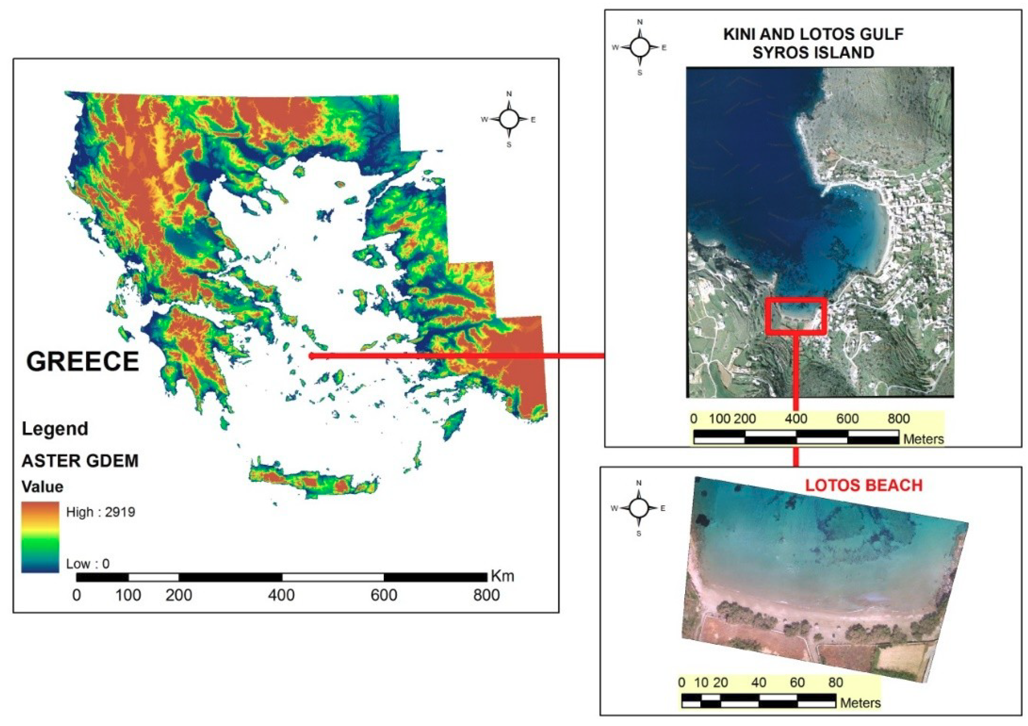
2. Geological Setting

The island of Syros is chiefly made up of rocks of the Blueschist Unit of the Cycladic Massif. This unit is mainly composed of marbles, schists, metabasites, and paragneisses [47], which have been subjected to Eocene (~53 Ma) eclogite- to blueschist-facies metamorphism followed by greenschist-facies retrogression in the late Oligocene–early Miocene [48] about 25–21 Ma. The Blueschist Unit is structurally overlain by the Uppermost Unit, also known as Vari Unit in local literature. The Vari Unit is exposed as a klippen in the southeastern coast of the island and consists mainly of felsic orthogneisses, quartz and quartzofeldspathic schists, mica schists, and metabasic schists, showing no evidence of Eocene high-pressure metamorphism [49]. Particularly, in the Lotos Gulf study area, as shown in Figure 1, there are exposed rocks of the Blueschist Unit and specifically greenschists, marbles, mica schists, and metabasites [47].
The tectonic contact between the Blueschist and the Vari Unit represents a passive normal-sense roof detachment (Vari Detachment), which was formed during northeast-directed ductile extrusion of the former at middle Eocene–Oligocene times [49]. Brittle-stage deformation is associated with the formation of faults resulted by a regional regime of SW-NE to WSW-ENE directed extension.

3. Survey Design

The integrated survey of Syros Island shallow waters beachrock was organized into three phases. During the first phase, a systematic survey of the seafloor using UAV and USV was carried out. The second phase of the survey consisted of the evaluation of the collected data of the UAV and USV using a GNSS receiver and was planned on the results of the first phase. During the third phase, rock samples were collected from specific sites of beachrock for further mineralogical analyses and petrographic studies. This methodological approach provides a cost-effective tool to rapidly survey areas of shallow water beachrock.
RGB images collected with a small commercial quadcopter were processed using Structure from Motion (SFM) photogrammetry in order to create digital surface models and orthophotos of the coastline. A beachrock lying in shallow waters was detected and mapped using the UAV-derived products. At the same time, a custom-made USV equipped with a compact side scan sonar (SSS) and a bathymetric sonar system, provided the exact shape of the beachrock, the latter extracted by mosaicking the backscatter strength of the SSS. SSS backscatter is long proven to be a valuable tool for mapping shallow water environments and is able to accurately delineate marine habitats [50] or any other regions of interest on the seafloor [51]. In order to evaluate the results of the UAV and USV data derivatives, the beachrock perimeter and its depth were also mapped using a differential global navigation satellite system (GNSS) receiver. The existence of different kinds of spatial information, raster data and vector data, points, polygons and polylines, necessitated the use of GIS software for the implementation, harmonization, and integration of the results. Firstly, the usefulness of the GIS is very clearly presented in the case of the GNSS survey. The UAV-derived digital surface models (DSMs) (raster data) were controlled with vector data (GNSS point measurements) and automatic algorithms were used for the vertical accuracy assessment. Furthermore, the USV survey data, SSS mosaic (raster) and bathymetric isolines (vector), point measurements from GNSS campaign, orthophoto and DSM from the UAV image processing, were integrated in GIS and produced the final maps. During the fieldwork, samples from the beachrock were collected for further analysis in the laboratory. The selection of the beachrock samples was based on the macroscopic observation of the lithology in the field. As the study area is quite small, only two samples with different macroscopic characteristics were selected. The mineralogical composition of the bulk samples was determined by powder X-ray diffraction (XRD). Mineralogical analyses and microstructure characterization were also performed using polarizing light microscopy, macroscope, and scanning electron microscopy (SEM).

4. UAV and USV Data Collection and Processing, Field Sampling

Diverse flight campaigns were planned and performed using a DJI Phantom 3 Advanced quadcopter (DJI, Guangdong, China) at different altitudes above ground level (agl). Photogrammetric grids were planned and executed at 20, 25, and 30 m agl, as shown in Figure 2. At the same time, the USV performed multiple waylines parallel to the coastline, in order to collect SSS data. Sample collection from different parts of the beachrock was also performed.

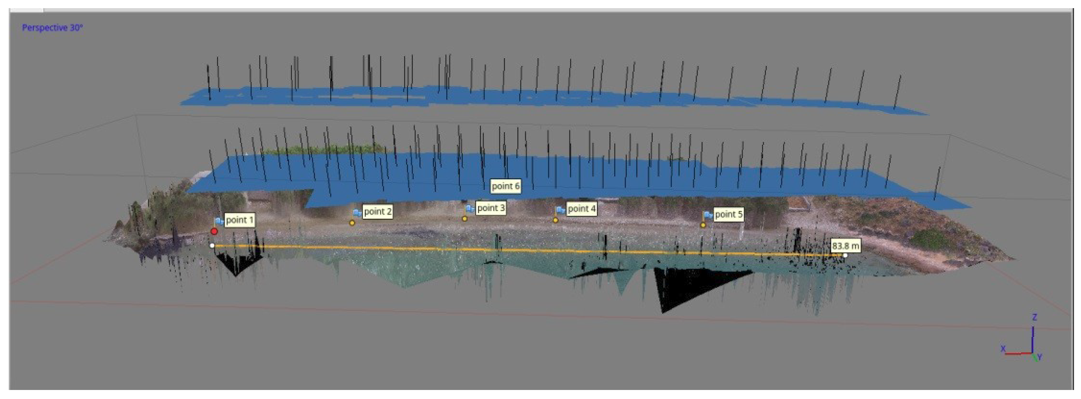
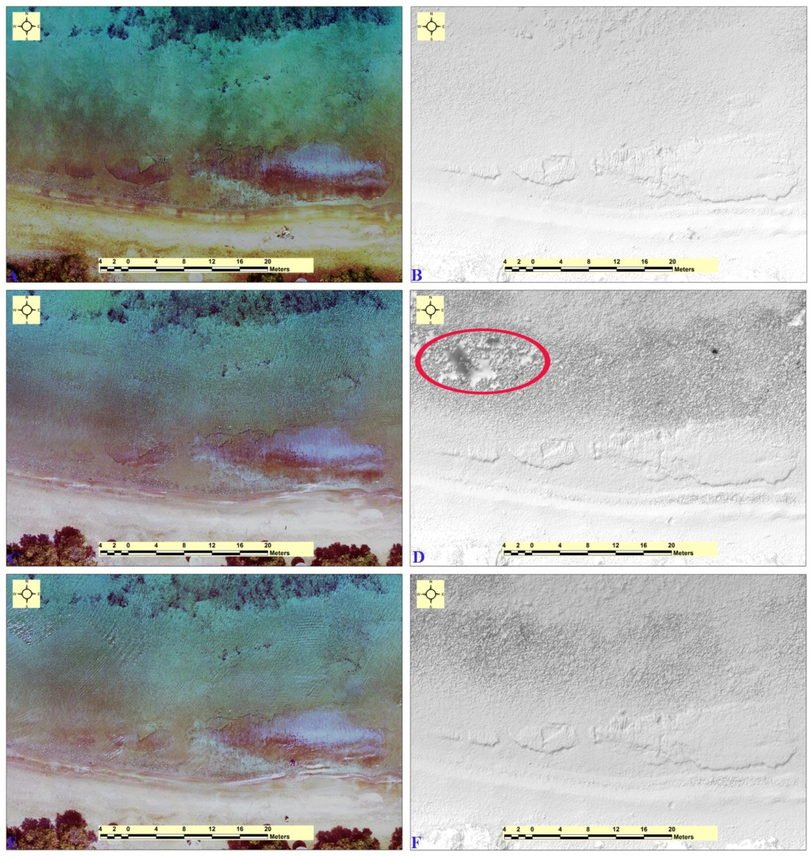
4.1. UAV Data Processing

The diverse datasets from the UAV flight campaigns at three different altitudes were imported in Agisoft’s PhotoScan software. In Figure 2, the allocation of the images acquired at 20 and at 30 m agl is presented. The allocation of the flight performed at 25 m altitude is not presented intentionally as the great number of images creates a confusing image. As described in detail in previous studies [52,53], the software combines computer vision techniques and Structure from Motion (SFM) photogrammetry in order to achieve direct georeferencing or bundle adjustment with ground control points (GCPs) or simple similarity transformation over the whole block without GCPs.
Similar to the traditional stereoscopic photogrammetry, SFM photogrammetry utilizes overlapping images acquired from different viewpoints. The basic difference of SFM photogrammetry to traditional photogrammetric approaches is that SFM determines internal camera geometry, camera position, and orientation automatically, and without the need to specify a priori, a network of targets which have known 3-D positions [54]. All these internal orientation parameters are calculated simultaneously using an iterative bundle adjustment procedure. The bundle adjustment is based on the automatic extraction of common features from a set of multiple overlapping images. As the number of acquired images increase, more and more points are correlated and ameliorate the internal block geometry. The need for a high degree of overlap to cover the full geometry of the object or scene of interest gives rise to the name: structure derived from a moving sensor.
In order to achieve the higher possible accuracy of the derived products, six artificial targets were scattered on the beach in order to be used as GCPs. The coordinates and height of each of these targets were measured using a high-accuracy geodetic GNSS receiver in order to ensure accurate positioning in Greece’s Coordinate System (EGSA 1987, EPSG 2100). The exact location of the ground control points is presented in Figure 2. The GCPs were spread around on the beach and not underwater as the total width of the study area is less than 100 m, as shown in Figure 2, and the relief is flat.
The three different image sets were processed in Agisoft PhotoScan as separate chunks. From the UAV data processing, orthophotos and digital surface models (DSMs) were created, as shown in Figure 3. The exact number of photos captured within every flight and the spatial resolution of the derived products are presented in Table 1. For the three flight campaigns at 20, 25, and 30 m agl, the same GCPs were used. The spatial resolution of the orthophotos ranges from 0.93 to 1.279 cm while the pixel size of the DSMs ranges between 1.86 and 2.558 cm. As the spatial resolution of the three orthophotos was quite similar, it was decided to export all the orthophotos at the same spatial resolution of 1 cm in order to facilitate the comparison. The common spatial resolution of the derived DSMs was decided to be 2 cm. In Figure 3, the orthophotos and the DSMs produced from the UAV data are presented. In the left column, the orthophotos from the images acquired at 20 m, as shown in Figure 3A, 25 m, as shown in Figure 3C, and 30 m, as shown in Figure 3E, and at the right column, the respective DSMs are presented, as shown in Figure 3B,D,F. The DSM from the UAV flight at 25 m agl is presented in Figure 3D. A red ellipse marks an artefact inside the specific DSM. In Figure 3E, the existence of light waves can be seen. Due to those waves the quality of the DSM in Figure 3F is not very high. However, the beachrock can be clearly detected in all the DSMs regardless of the flight altitude and the overall quality of the DSM. The 3-D model from the flight campaign at 20 m agl presented the higher horizontal and vertical accuracy, as shown in Table 2, and it was used for further processing and measurements. The easting (X) error was 2.07482 cm while the northing (Y) was a little higher (2.83607 cm). The altitude error (Z) was 2.245343 cm while the total root mean square error was 4.1752298 cm.
UAV data showed that the beachrock formation is fragmented to one extended and three smaller blocks. In the three DSMs, as shown in Figure 3B,D,F, the fragmented beachrock appears as a low relief ridge on the seabed running parallel/subparallel to the present day coastline. The increase in the flight altitude from 20 m, as shown in Figure 3B, to 30 m, as shown in Figure 3F, did not affect the visibility of the beachrock on DSMs. The four blocks of the fragmented beachrock can be easily distinguished. As the orthophoto and the DSM from lower flights are clearer, they have been used for further processing and measurements. The most laterally extensive block of beachrock lies at the eastern end of the formation and covers an area of 176 square meters, having a maximum length of 30 m and a maximum width of 10 m. The extent of the other three blocks is 27, 10, and 11 square meters, respectively. Those three blocks have a maximum length of 9.8, 4.8, and 3.9 m, and a maximum width of 4, 1.5, and 1 m, respectively.
The orthophotos were further processed using ERDAS IMAGINE software. Different processing techniques, like image enhancement and filtering, were applied to the data in order to enhance the visibility of the beachrock and improve its traceability. In Figure 4, the digitally processed orthophotos of the 20 m agl flight are presented. Figure 4A shows the orthophoto after sharpness and contrast enhancement. More precisely, the image was stretched evenly between plus and minus two standard deviations around the mean and then the contrast was increased about 20%. Figure 4B presents the result of the filtering to the previous orthophoto, as shown in Figure 4A. A standard edge enhancement filter was applied to the image. The fragmented beachrock formation is presented with reddish tones in the orthophotos of Figure 4. The specific color difference facilitates the mapping of the beachrock extents but it does not permit the automatic detection and classification of it. The existence of the specific beachrock is certified, also taking into account all the other data. The black points in Figure 4B represent the GNSS measurements, while points 1 and 2 in Figure 4A represent the positions of the field sampling.
From a coastal morphodynamics point of view, the fragmented beachrock formation constitutes a coastal shallow barrier that influences the local littoral transport processes. As it can be observed in Figure 4A,B, coarse-grained (gravel) sediments have been accumulated between the beachrock and the shoreline. The existence of the beachrock formation locally weakens the incoming wave energy and consequently alters the longshore sediment drift. As the beachrock is fragmented in one extended and three smaller blocks, it cannot serve as an elongated unique barrier and filter wave energy, but as four independent blocks. The deposition and aggregation of coarse-grained sediments follows, in general, the shape of the fragmented beachrock formation. Four separate cones of gravelly material have been deposited between the beachrock and the shoreline while sandy corridors have developed between them. This observation is in accordance with previous work [16].

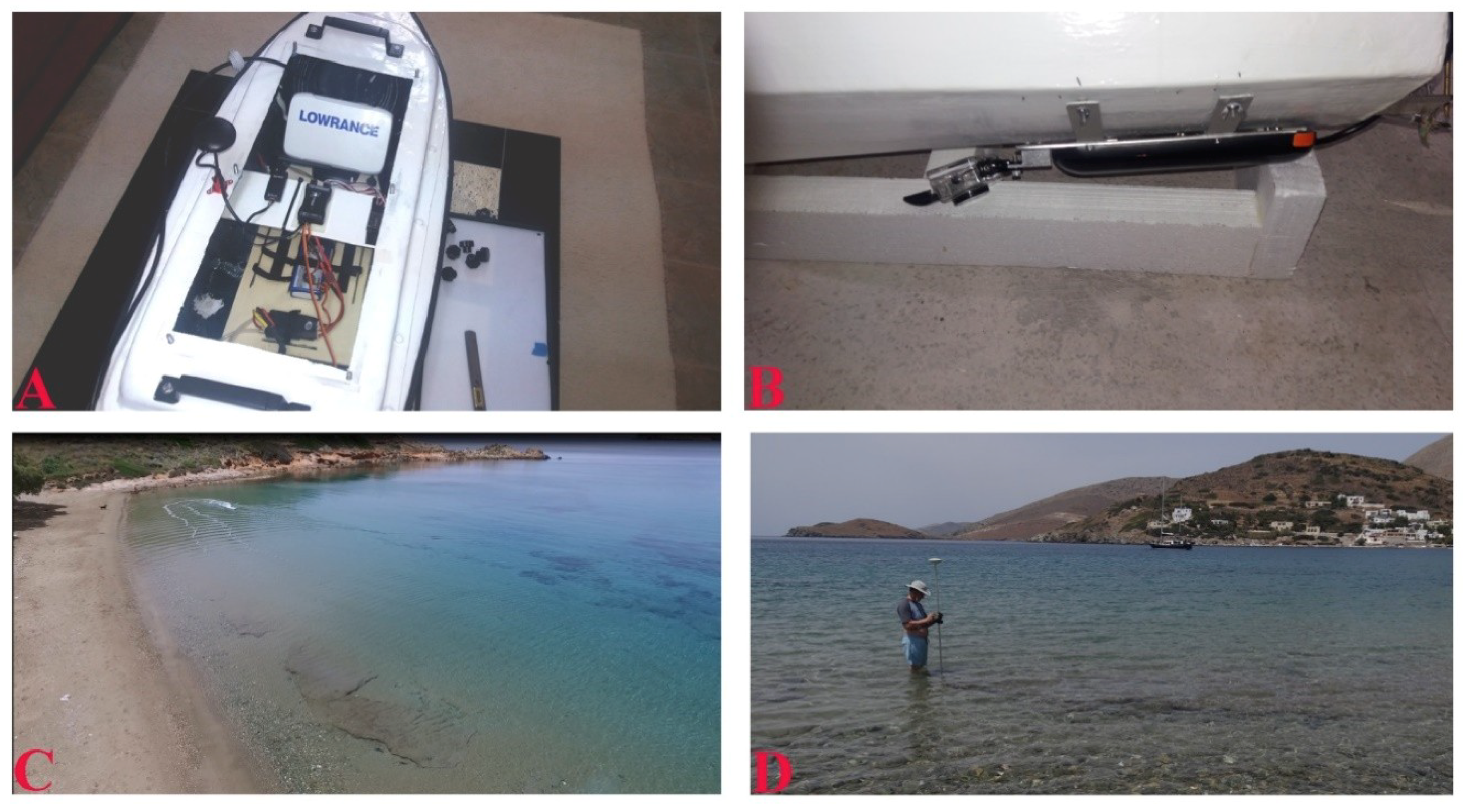
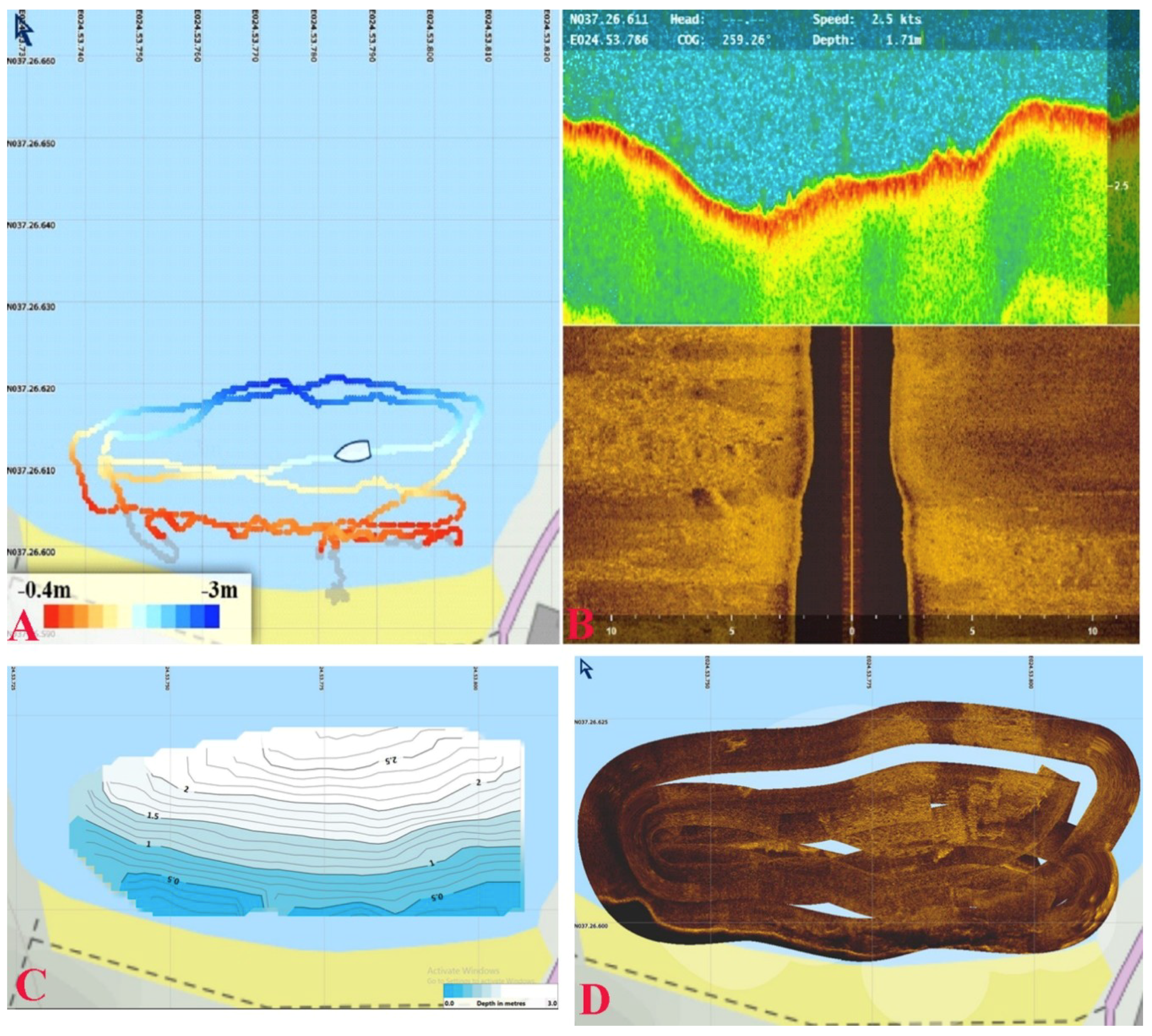
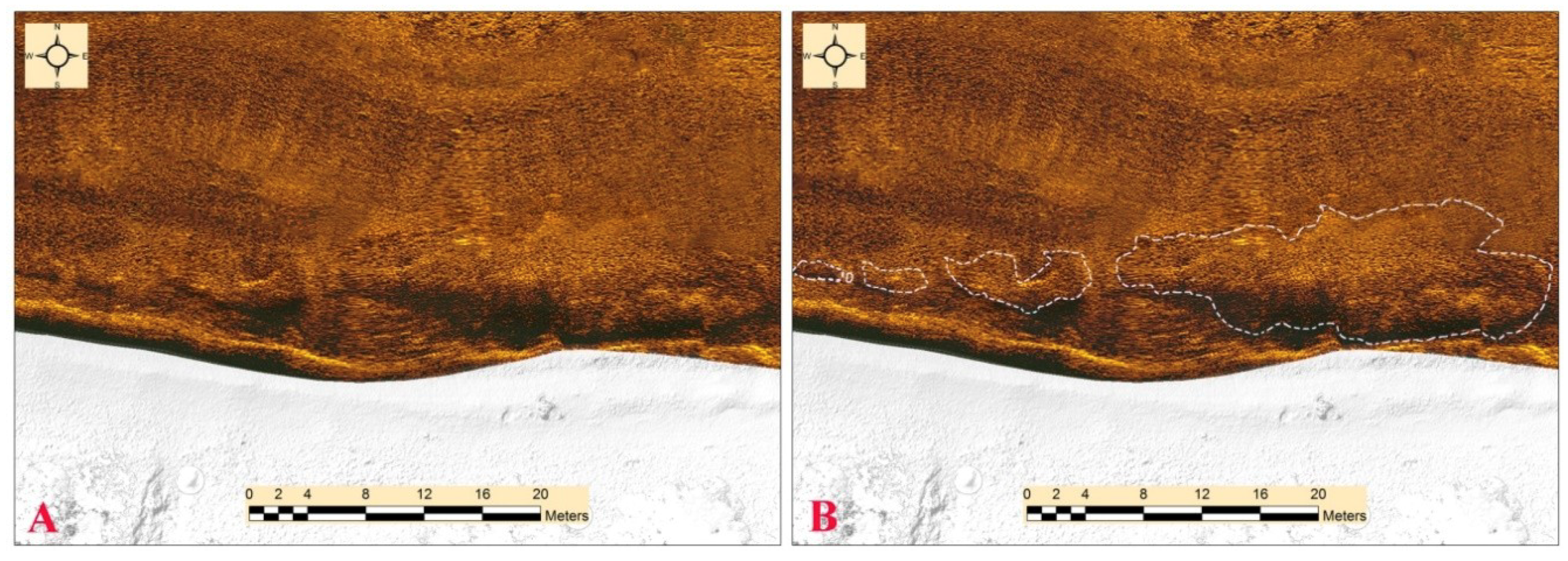
4.2. USV Data Collection and Processing

Although marine remote sensing surveys are typically performed using research vessels, for the survey of the very shallow water, small surface vehicles are required. USVs are cost effective and easily transported to the field. They are well suited for demanding environments, such as shallow lakes, rivers, aqueducts, canals, and lagoons, and they can reach areas close to piers, pilings, and the extremely shallow waters at the coastal zone [55,56,57,58].
A custom-made, small (1 m long) remotely operated USV was used for retrieving shallow geoacoustic data, as shown in Figure 5C. It offers efficient simultaneous bathymetry and side scan mapping in waters as shallow as 40 cm, allowing surveying in locations and environmental conditions in which deployment of conventional platforms is not practicable or feasible. It features a fully autonomous GPS waypoint-based navigation system with a real-time telemetry link. The USV platform is customizable, allowing it to accept existing GPS/real-time kinematic (RTK) positioning systems, bathymetric sonars, SSS, and video cameras. It is currently equipped with an 83/200 kHz broadband chirp single beam bathymetric sonar and a 455/800 kHz SSS, both integrated in the Lowrance Elite-7 Ti sonar, as shown in Figure 5A, and a hull-mounted High Definition (HD) underwater camera for very shallow seafloor mapping and visual inspection, as shown in Figure 5B. All instrumentation is synchronized and linked to an external high precision GPS system, to offer fully georeferenced and co-registered geoacoustic and video footage data. A video presenting the data collection with the USV can be found in the Supplementary Materials.
The SSS and bathymetric datasets were processed using the ReefMaster software tool (Reef Master Software Ltd, West Sussex, UK). A bathymetric map and an SSS mosaic were also constructed using ReefMaster, as shown in Figure 6. The agreement between the geoacoustically-derived bathymetry data and the GNSS elevation measurements is out of the scope of the current work, as it would need further correction of the bathymetric data with regard to the tidal variations during the sampling period. High backscatter, which is attributed to hard substrate, is presented by light tones on sonographs whilst low backscatter (soft substrate) is presented by dark tones. Figure 6C presents the bathymetric map in the area of beachrocks; the beachrock formations lie at a water depth ranging from 0.0 to 0.7 m. Figure 6D show the SSS mosaic in the area of the beachrock, and Figure 7 presents a detailed SSS sonograph showing the four fragments of the beachrock formation. The four separate beachrock fragments are clearly enough delineated through the relatively higher backscatter intensity compared to the surrounding seafloor. Moreover, the dark-toned acoustic shadow that has developed due to the high incidence angle between the transmitted acoustic signal and the seabed clearly delineates the southern end of the beachrock, as shown in Figure 7.

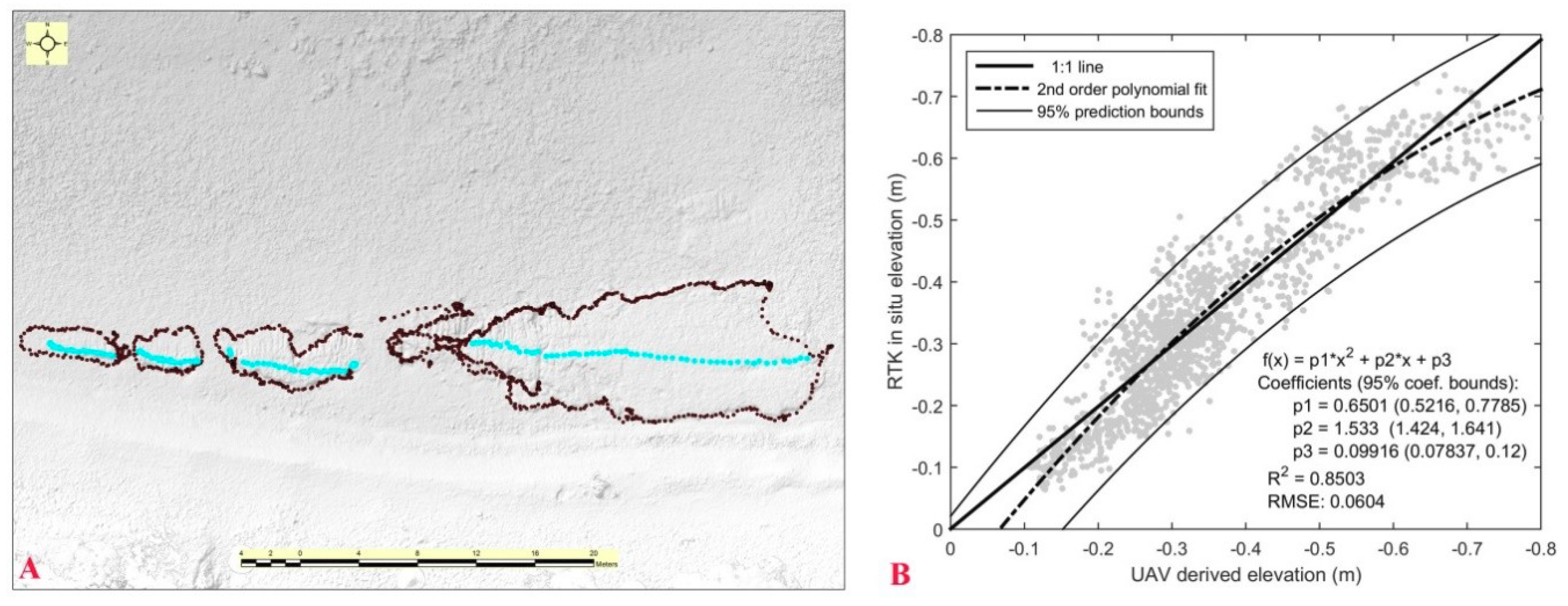
5. GNSS Measurements

During the fieldwork, 1440 points were collected with a Leica GS08 Plus GNSS receiver. The receiver was used without a dedicated base station, but with differential position corrections from the Metricanet network—through Global System for Mobile Communications (GSM) and real-time kinematic (RTK). Metricanet is the local partner in Greece of HxGN SmartNet. HxGN SmartNet is the GNSS correction service built on the world’s largest reference station network (more than 4000 reference stations based on Leica Geosystems), enabling GNSS-capable devices to quickly determine precise positions even down to the centimeter.
The receiver used in the field is capable of GPS (L1, L2, and L2C frequencies), Globalnaya Navigazionnaya Sputnikovaya Sistema (GLONASS, L1 and L2 frequencies), and Satellite-based Augmentation Systems (SBAS) (Wide Area Augmentation System (WAAS), GPS Aided Geo Augmented Navigation (GAGAN), Multi-functional Satellite Augmentation System (MSAS), and European Geostationary Navigation Overlay Service (EGNOS) systems). The accuracy specifications for this receiver are 10 mm + 1 ppm horizontally and 20 mm + 1 ppm vertically. During the GCPs’ measurements, the horizontal root mean squared error (RMSE) was between 0.6 and 1.0 cm, whereas the vertical RMSE between 1.1 and 1.6 cm.
The majority of the GNSS measurements were taken in the shallow water covering the extent of the fragmented beachrock formation, as shown in Figure 5D. Measurements were also acquired on the “crest line” of the beachrock, producing east to west sections, as shown in Figure 8a. The crest line of the fragmented beachrock formation, ranges between from −0.08 to −0.028 m below sea surface. The beachrock lies in depths between −0.03 to −0.734 m below sea surface.
The DSM of the lower altitude UAV’s flight (20 m) was validated against the GNSS measurements. Comparison between the above two data sets offered the means for calibrating the DSM, suggesting a simple linear regression for correcting the water column effect on the elevation estimations. Figure 8B shows the agreement between the DSM and the GNSS altitudes, with the 1:1 line indicating the linear regression used for the DSM calibration. A further 2nd order polynomial seems to further improve the DSM agreement with the GNSS measurements, but with a negligible effect on the actual results. The root mean squared error (RMSE) of the regression is 6 cm while the R2 is 0.85, suggesting a strong correlation between the DSM and the GNSS elevation values, which suffers though from quite high deviation around the regression line. Further calibration of the UAV-derived elevation model is out of the scope of this work.

6. Mineralogical and Petrographic Analyses

6.1. Analytical Methods

A laboratory qualitative petrographic study of selected samples was conducted by several combined petrographic methods. The bulk mineralogical composition of the studied samples was determined with X-ray diffraction using a Bruker D8 advance diffractometer (with ~3% resolution), equipped with a LynxEye1 detector with Ni-filtered CuKα radiation, accelerating at 40 kV, 40 mA. Random powder mounts were prepared by gently pressing the powder into the cavity holder. The scanning area for bulk mineralogy of specimens covered the 2θ interval 2°–70°, with a scanning angle step size of 0.015° and a time step of 0.1 s. The mineral phases were determined using the DIFFRACplus EVA 12® software (Bruker-AXS, Fitchburg, WI, USA) based on the ICDD Powder Diffraction File of PDF-2 2006. The mineralogical and textural characteristics of the samples were also examined on polished thin sections using a petrographic polarizing microscope (Leica Microsystems, Leitz Wetzlar, Germany). The microfossils have also been observed in polished thin sections under a macroscope Wild Heerbrugg M400.
Furthermore, a petrographic study by a scanning electron microscope SEM JEOL 6300 equipped with an energy dispersive spectrometer (EDS) (accelerating at 20 kV) on gold and/or carbon-coated freshly randomly broken surfaces of samples, as well as on carbon-coated thin sections, was conducted. Secondary electron images (SEI) (on freshly randomly broken surfaces of samples), backscattered electron scanning images (BSE-SEM) (on polished thin sections), as well as BSE-EDS microanalysis (on polished thin sections), are presented in this study.
Two samples of each area were prepared for XRD analysis, petrographic study under polarizing microscope and macroscope, as well as for BSE-SEM analysis, and representative results are presented in this study. Moreover, fragments from the initial collected samples have been broken randomly and five pieces from each area were analyzed using SEM, and representative results are provided.

6.2. Mineralogical Analyses and Microstructures

6.2.1. XRD Analysis

The qualitative analyses by XRD technique, as shown in Figure 9, of the two beachrock collected samples, as shown in Figure 4A, revealed similar mineral phases comprising: quartz, calcite, alkali feldspars (albite), pyroxene, epidote group minerals (epidote, zoisite), green, blue amphibole (glaucophane, actinolite), mica (muscovite and/or illite), and chlorite. These phases reflect the bedrocks of this region in which there were constituents before erosion and weathering (mainly metamorphic rocks of Syros Island).

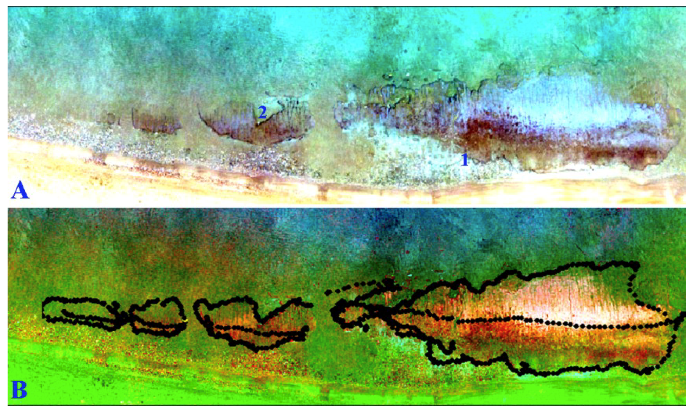
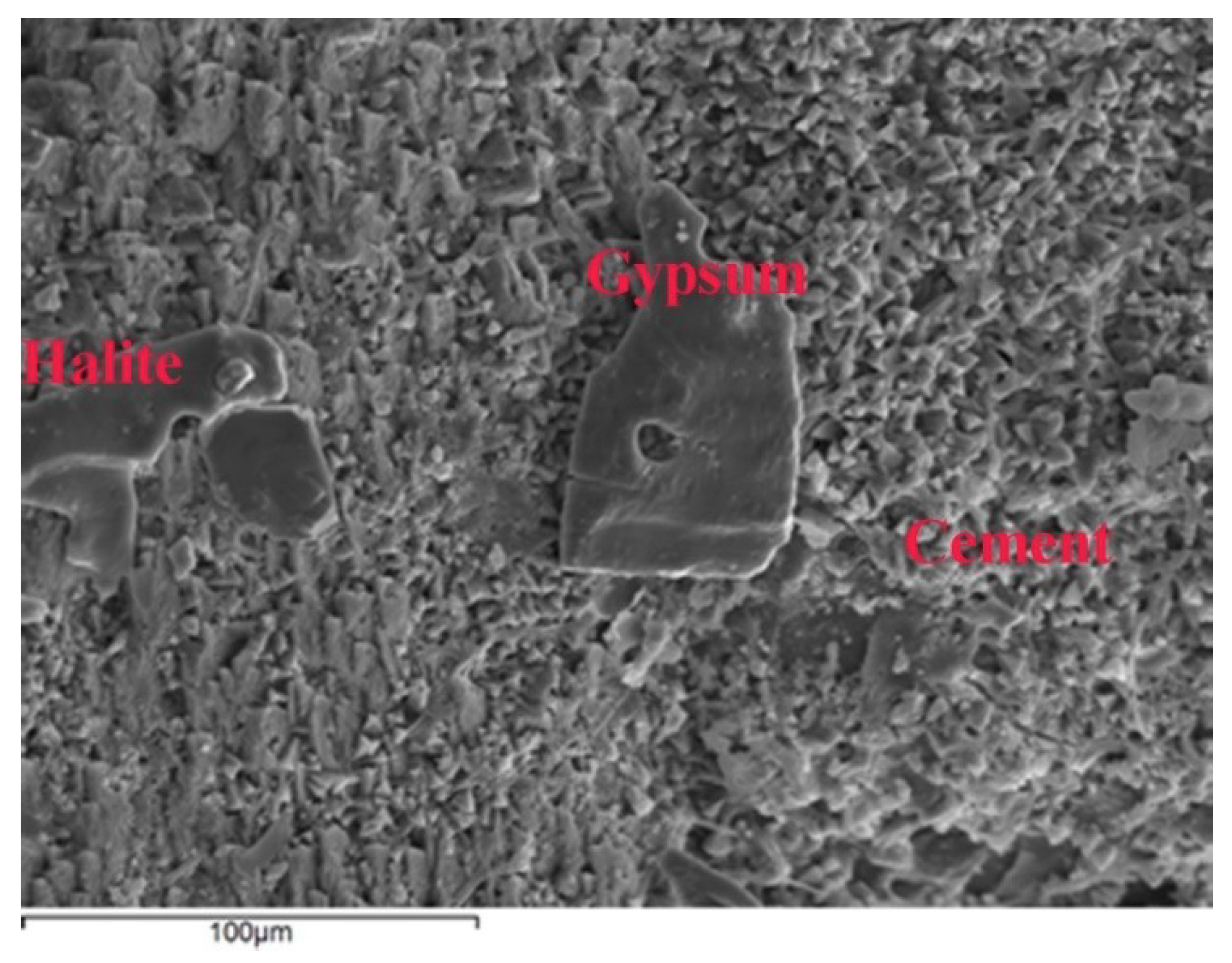
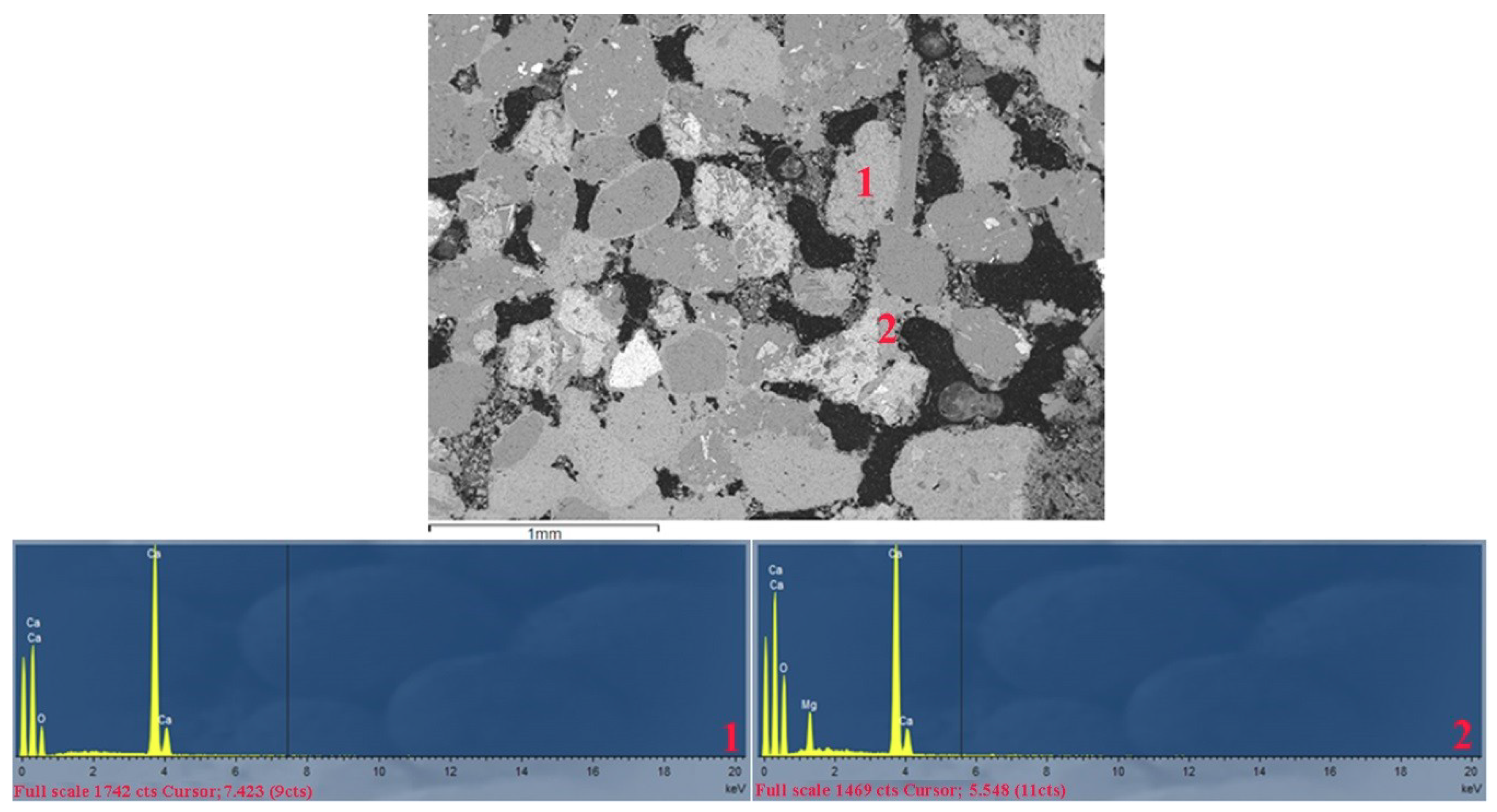
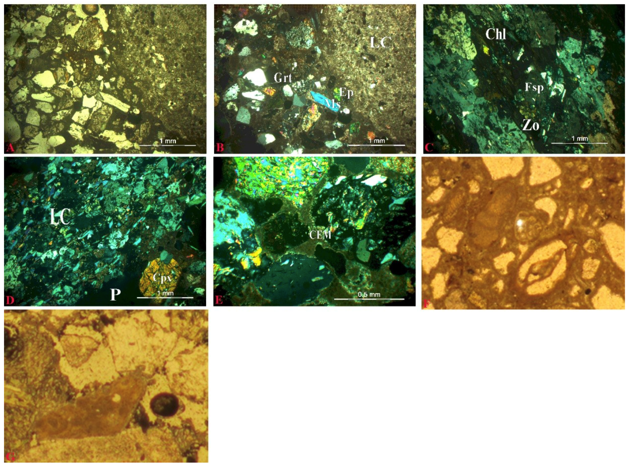
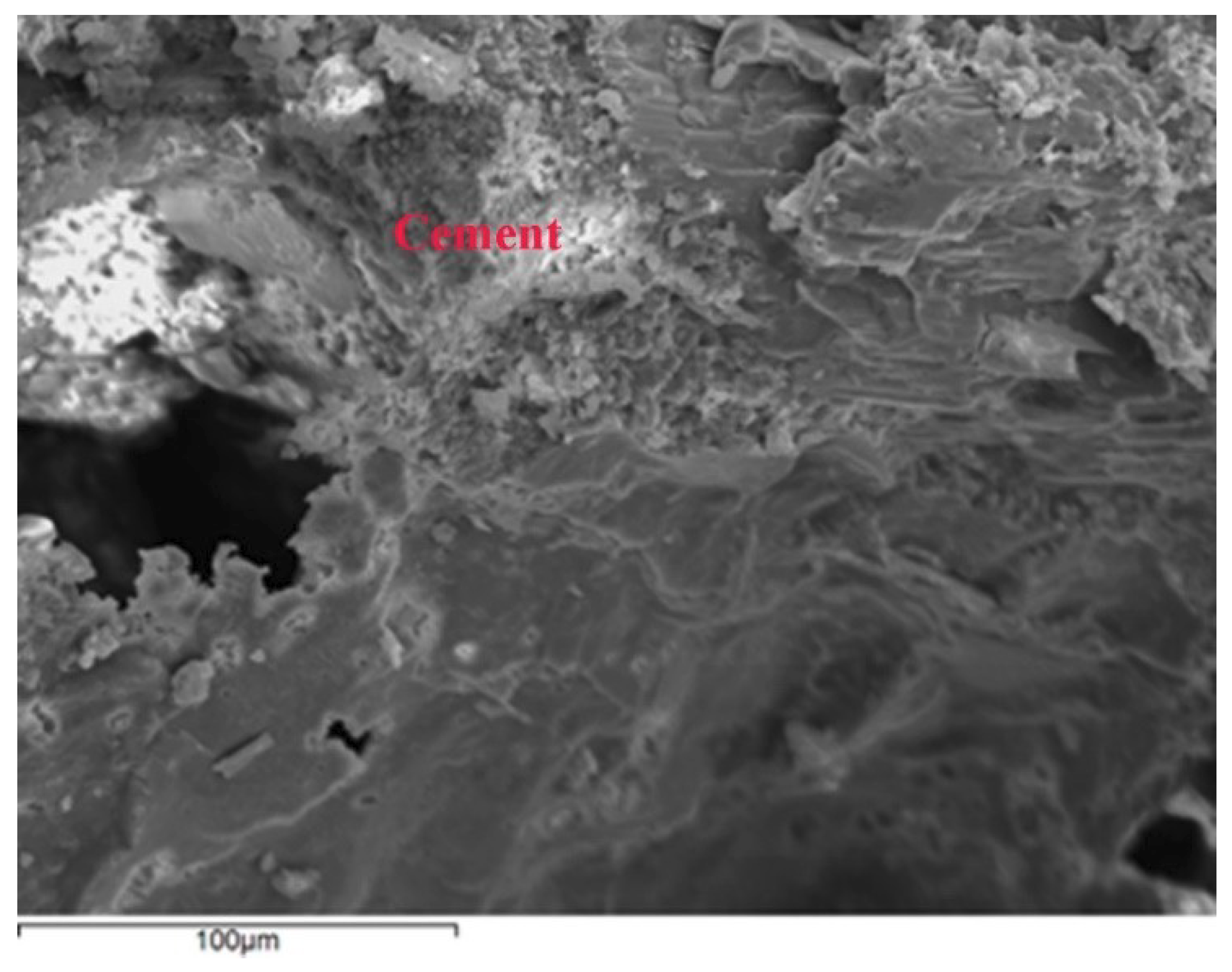
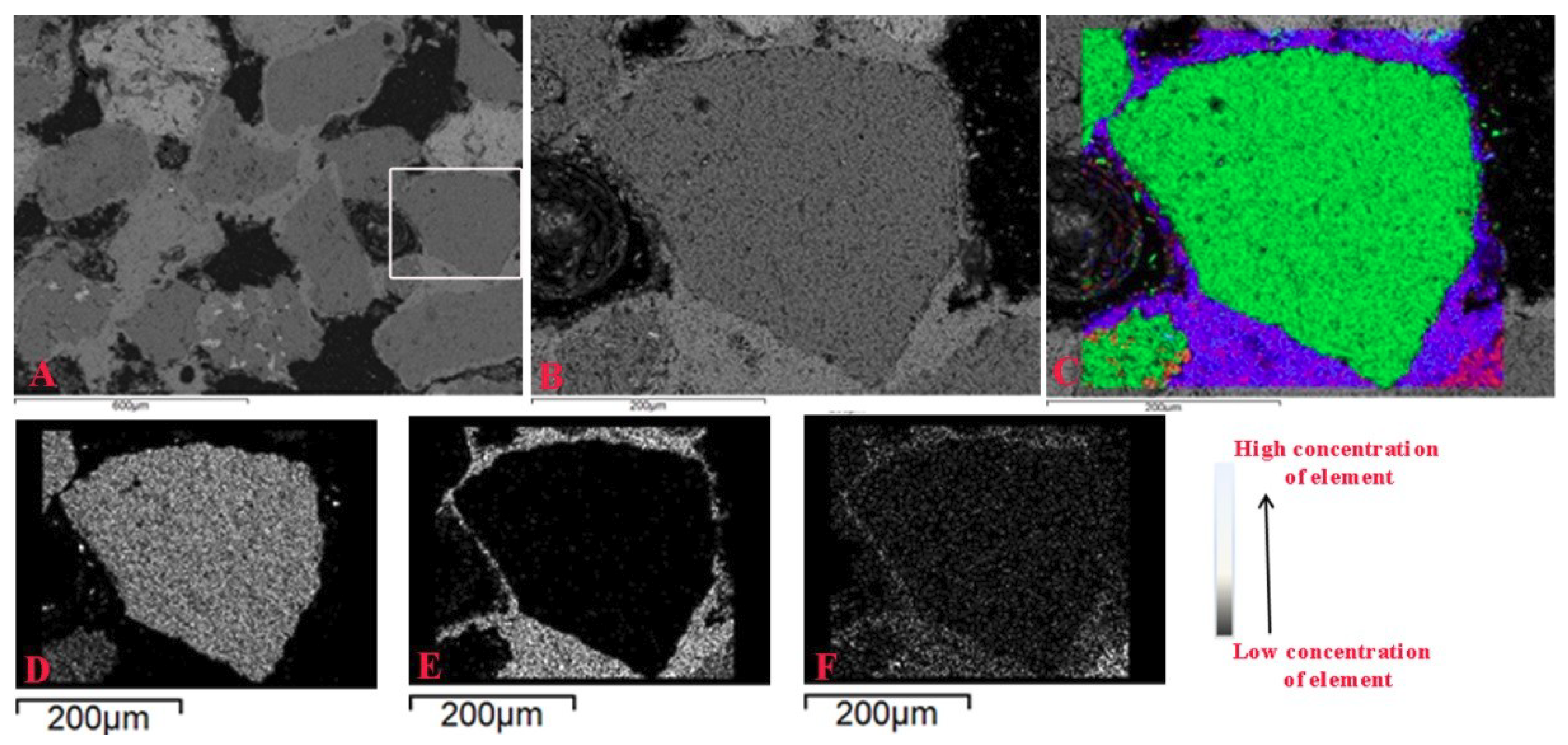
6.2.2. Petrographic Features under Petrographic Polarizing Microscope and SEM Analysis

Beachrock samples of area 1, as shown in Figure 4A, are classified as fine to medium grain sandstones with clastic texture and good sorting. They consist mainly of sub rounded grains of minerals, lithoclasts, and bioclasts (fragments of mollusk shells, foraminifera, small gastropods, bone fragments, and algae), and are shown in Figure 10A–H. All of these phases are mainly cemented by micritic carbonates.
The dominated grains observed under microscopy are quartz, carbonates, feldspars, pyroxene, and epidote-zoisite, while less abundant phases are mica (muscovite), chlorite, green, blue amphibole (glaucophane, actinolite), garnet, and opaque minerals. Accessory phases of sphene and spinel are also presented in mineral composition. Moreover, fine halite and gypsum detected by SEM to coexist with micritic carbonates, as shown in Figure 11. The presence of halite and gypsum could also be due to sample processing since the sample was air dried and, moreover, these phases were not detected by XRD. The lithoclasts are mainly fragments of mica schists, chlorite schists, and carbonate rocks, mainly marbles derived from the broad area rock units. Quartz crystals exhibit undulose extinction indicating intracrystalline deformation phenomena. Occasionally feldspars show partial transformation to sericite. The occurrence of cracked pyroxene altered to chlorite and filled with oxides and other minerals is frequently observed. Most garnet crystals are intensively cracked and preferentially replaced by chlorite.
Several studies have referenced the different types of cement textures of these rocks [3,14,59,60,61]. In the case of samples of area 1, they have been cemented by micrite carbonates filling pores or forming meniscus bridges between the grains or fragments, as shown in Figure 10D,E. Moreover, the majority of the grains and lithoclasts throughout the microstructure are surrounded by micritic material, as shown in Figure 10E, which is a very frequent cement texture of beachrocks [14], whilst peloidal aggregates are also observed, as shown in Figure 10F. Sometimes recrystallized micrite to sparite is presented, indicating a more stable thermodynamic state, as shown in Figure 10D. The secondary electron image of Figure 11 shows the micritic morphology of cement in beachrocks of area 1. The backscattered electron image, as shown in Figure 12, presents clearly the textural characteristics of microstructure and how cement bonds grains together or coats others. The majority of the detrital carbonate grains of these studied rocks consist of pure calcite mineralogy free of magnesium, as it is observed with the representative EDS spectrum 1 of Figure 12. On the contrary, the cement indicates a magnesium–calcium chemistry.
A number of BSE-EDS microanalyses (~30) of the cement phase of area 1 beachrock have been carried out in several micro-regions, such as in Figure 12, in polished thin section samples, and representatives of these are given in Table 3. The whole wt. % data collected using EDS analysis were used to calculate the mol % of MgCO3, which is present in the cement phase and the extreme and mean values of them are given also in Table 3. The results show that the mol % of MgCO3 in cement phase of samples of area 1 ranges from 4% to 16%, characterizing this as high magnesium calcite (HMC). Generally, the cement phases of such rocks are mainly calcite or aragonite [44,59]. The precipitation and composition of these phases depend on a variety of physicochemical parameters, e.g., temperature, pH, salinity, and Mg2+ concentration. Besides these factors, recent studies revealed that the presence of microorganisms play a severe role in the formation of beachrocks as these enhance the dissolution of carbonate grains, increasing the cation in solution leading to precipitation [4,5]. In the case of area 1, textural characteristics of cement in combination with its HMC composition are probably indicating that the beachrock was formed under marine-vadose conditions [1,13]. The contribution of organism activity to cement formation should not be rejected but further investigation with high-resolution techniques is demanded, e.g., References [4,5].
Beachrock samples of area 2, as shown in Figure 13A–G, can be described as conglomerates comprising mainly of sub angular to sub rounded lithoclasts (epidote-chlorite schists, mica schists, carbonate rocks). The sand matrix participates in lower amounts, presenting similar mineralogical and textural characteristics with sandstones (beachrock samples) of area 1, as shown in Figure 10. Microfossils in the microstructure of these beachrocks were also observed under macroscope and representative images are presented in Figure 13F,G.
The different sorting characteristics of collected beachrock samples of area 2, which are as far apart as a few meters (~20 m) from these of area 1, could be attributed either to a mechanism similar to the one described in above sections or to lower reworking during transporting due to the proximity of an additional source area to the sea coast. The latter could have been a hydrographic system having its estuary in this area and may have contributed to the transporting ability of coarser fragments from different sources (compared to these of area 1), promoting the immature character of these beachrocks.
Concerning the consolidation texture of these rocks, even though the sand acts as cement (between lithoclasts), micritic carbonates have also been precipitated, coating the sand grains and fragments or forming bridges between particles while peloids have also been observed, as shown in Figure 13E. Nevertheless, in the case of area 2 samples, the micritic carbonates around the coarser particles are lesser compared to the fine ones, due to their low surface free energy.
The morphology of micritic cement is presented in the secondary electron image of Figure 14. Elemental mapping was carried out in a part of the micro region of the BSE-SEM image of Figure 15 where cement is coating a quartz grain. In this case of Si, Ca, and Mg analysis, the information of magnesium participation in calcite cement was also provided as in area 1.
Approximately 30 BSE-EDS analyses collected on polished thin sections pointed out that HMC with ~15 mol % MgCO3 in solid solution formed the cement, as shown in Table 3. Representative microanalyses are given in Table 3.
According to the above results, similar texture and cement composition with those of area 1 rocks contribute to the approach that area 2 rock formations are also related to an environment of a marine-vadose zone.

7. Discussion and Conclusions

In this study, a synergy of different geological specialties is proposed, combining UAV and USV data, mineralogical analyses, GNSS measurements, and geographic information systems for the detection, mapping, and further characterization of a fragmented beachrock formation lying on very shallow waters (0–0.7 m) in Lotos beach, Syros Island.
One main concept of this study was to use low-cost, customer-grade UAV and USV equipment as a tool for quick beachrock detection and mapping. The use of low-cost UAVs has been recently exhibited in previous works (e.g., Reference [28]). In the same manner, recreational grade sonars (e.g., the Lowrance fish-finders) are increasingly being used for deriving scientific seafloor mapping (e.g., Reference [62]). Although the beachrock was actually quite well delineated in both the UAV or SSS derived products, especially when outlined by experienced interpreters, their synergistic use proved to be beneficial. If there should be a trade-off between human–effort and detection accuracy, this would most likely favor aerial surveys rather than sidescan surveys due to the difficulty in SSS interpretation. This, however, does not mean that a combination of both the above very low-cost systems would not offer increased beachrock delineation significances. In some cases, SSS could be even more successful in detecting very shallow seabed features than using an aerial survey, especially in very nontransparent waters (i.e., with increased amounts of suspended sediments) or in cases where the sea-surface sun-glint is high, see Figure 3. On the contrary, SFM via UAV imagery offers the means for an easy visual interpretation as it provides images familiar to the human eye, along with a 3-D representation.
It has been proven that both UAV with Structure from Motion photogrammetry, and USV with side scan sonar and echo sounder, can detect and map morphological features in shallow waters where conventional research vessel and platforms cannot be applied. Furthermore, the combination of the petrography and mineralogy analyses with remote sensing methodologies revealed not only the spatial extent of each formation but also the precise composition of the beachrock, giving insights about their formation mechanisms. Finally, GIS technology was necessary for the homogenization and processing of different raster and vector data, and the production of the respective maps.

Supplementary Materials

The following are available online at https://www.mdpi.com/2075-163X/8/11/534/s1, Video S1: Unmanned Surface Vehicle data collection from Unmanned Aerial Vehicle.

Author Contributions

K.G.N. has conceptualized this work and has performed UAV data collection, GNSS measurements, remote sensing data processing, and spatial analysis in GIS. He wrote the respective parts in the current paper. P.L. carried out all the petrographic and mineralogical analyses of the samples and she wrote the respective parts of the current paper. E.F. processed the USV data and contributed to the respective parts in writing. D.S. designed the USV in collaboration with K.G.N., and E.F. took over its development and contributed to the USV data collection. G.P. participated in the fieldwork and wrote parts of this paper.

Funding

Part of this research was co-financed by the European Union (EU Environmental Funding Programme LIFE+ Environment Policy and Governance) and Greek national funds through the LIFE DEBAG project “Integrated information and awareness campaign for the reduction of plastic bags in the marine environment” (LIFE14 GIE/GR/001127). The funders had no role in the study design, data collection and analysis, decision to publish, or preparation of the manuscript.

Acknowledgments

The authors would like to thank the members of the Laboratory of Marine Geology and Physical Oceanography for their support during the fieldwork, A.K Seferlis of the Laboratory of Electron Microscopy and Microanalysis, University of Patras for his assistance with the microanalyses and SEM micrographs, and Associate Professor George Iliopoulos for his assistance with the bioclast analyses. Authors are grateful to the three anonymous reviewers for their valuable comments and annotations that helped improve the quality of this article.

Conflicts of Interest

The authors declare no conflict of interest.

References

  1. Mauz, B.; Vacchi, M.; Green, A.; Hoffmann, G.; Cooper, A. Beachrock: A tool for reconstructing relative sea level in the far-field. Mar. Geol. 2015, 362, 1–16. [Google Scholar] [CrossRef]
  2. Alexandersson, T. Recent littoral and sublittoral high-Mg calcite lithification in the Mediterranean. Sedimentology 1969, 12, 47–61. [Google Scholar] [CrossRef]
  3. Moore, C.H. Intertidal carbonate cementation Grand Cayman, West Indies. J. Sediment. Res. 1973, 43, 591–602. [Google Scholar]
  4. McCutcheon, J.; Nothdurft, L.D.; Webb, G.E.; Paterson, D.; Southam, G. Beachrock formation via microbial dissolution and re-precipitation of carbonate minerals. Mar. Geol. 2016, 382, 122–135. [Google Scholar] [CrossRef] [Green Version]
  5. McCutcheon, J.; Nothdurft, L.D.; Webba, G.E.; Shuster, J.; Nothdurfta, L.; Patersone, D.; Southama, G. Building biogenic beachrock: Visualizing microbially-mediated carbonate cement precipitation using XFM and a strontium tracer. Chem. Geol. 2017, 465, 21–34. [Google Scholar] [CrossRef] [Green Version]
  6. Cooper, J.A.G. Beachrock formation in low latitudes: Implications for coastal evolutionary models. Mar. Geol. 1991, 98, 145–154. [Google Scholar] [CrossRef]
  7. Caldas LHO; Stattegger, K.; Vital, H. Holocene sea-level history: Evidence from coastal sediments of the northern Rio Grande do Norte coast, NE Brazil. Mar. Geol. 2006; 228, 39–53. [Google Scholar]
  8. Vousdoukas, M.I.; Velegrakis, A.F.; Plomaritis, T.A. Beachrock occurrence, characteristics, formation mechanisms and impacts. Earth Sci. Rev. 2007, 85, 23–46. [Google Scholar] [CrossRef]
  9. Desruelles, S.; Fouache, É.; Ciner, A.; Dalongeville, R.; Pavlopoulos, K.; Kosun, E.; Coquinot, Y.; Potdevin, J.L. Beachrocks and sea level changes since Middle Holocene: Comparison between the insular group of Mykonos–Delos–Rhenia (Cyclades, Greece) and the southern coast of Turkey. Glob. Planet. Chang. 2009, 66, 19–33. [Google Scholar] [CrossRef]
  10. Hopley, D. Beachrock as a sea-level indicator. In Sea-Level Research; Van de Plassche, O., Ed.; Springer: Dordrecht, Germany, 1986; pp. 157–173. [Google Scholar]
  11. Mourtzas, N.D.; Kissas, C.; Kolaiti, E. Archaeological and geomorphological indicators of the historical sea level changes and the related palaeogeographical reconstruction of the ancient foreharbour of Lechaion, East Corinth Gulf (Greece). Quat. Int. 2014, 332, 151–171. [Google Scholar] [CrossRef]
  12. Ozturk, M.Z.; Erginal, A.E.; Kiyak, N.G.; Ozturk, T. Cement fabrics and optical luminescence ages of beachrock, North Cyprus: Implications for Holocene sea-level changes. Quat. Int. 2016, 401, 132–140. [Google Scholar] [CrossRef]
  13. Longman, M.W. Carbonate diagenetic textures from near surface diagenetic environments. AAPG Bull. 1980, 64, 461–487. [Google Scholar]
  14. Vieira, M.M.; De Ros, L.F. Cementation patterns and genetic implications of Holocene beachrocks from northeastern Brazil. Sediment. Geol. 2006, 192, 207–230. [Google Scholar] [CrossRef]
  15. Psomiadis, D.; Albanakis, K.; Zisi, N.; Ghilardi, M.; Dotsika, E. Clastic sedimentary features of beachrocks and their palaeo-environmental significance: Comparison of past and modern coastal regimes. Int. J. Sediment. Res. 2014, 29, 260–268. [Google Scholar] [CrossRef]
  16. Velegrakis, A.F.; Trygonis, V.; Chatzipavlis, A.E.; Karambas, T.; Vousdoukas, M.I.; Ghionis, G.; Monioudi, I.N.; Hasiotis, T.; Andreadis, O.; Psarros, F. Shoreline variability of an urban beach fronted by a beachrock reef from video imagery. Nat. Hazards 2016, 83, 201–222. [Google Scholar] [CrossRef]
  17. Vousdoukas, M.I.; Velegrakis, A.F.; Paul, M.; Dimitriadis, C.; Makrykosta, E.; Koutsoubas, D. Field observations and modeling of wave attenuation over colonized beachrocks. Cont. Shelf Res. 2012, 48, 100–109. [Google Scholar]
  18. Arrieta, N.; Goienaga, N.; Martínez-Arkarazo, I.; Murelaga, X.; Baceta, J.I.; Sarmiento, A.; Madariaga, J.M. Beachrock formation in temperate coastlines: Examples in sand-gravel beaches adjacent to the Nerbioi-Ibaizabal Estuary (Bilbao, Bay of Biscay, North of Spain). Spectrochim. Acta Part. A: Mol. Biomol. Spectrosc. 2011, 80, 55–65. [Google Scholar] [CrossRef] [PubMed]
  19. Erginal, A.E.; Kıyak, N.G.; Ozturk, M.Z.; Avcıoglu, M.; Bozcu, M.; Yigitbas, E. Cementation characteristics and age of beachrocks in a fresh-water environment, Lake Iznik, NW Turkey. Sediment. Geol. 2012, 243, 148–154. [Google Scholar] [CrossRef]
  20. Vincent, C. Contrasted textural and taphonomic properties of high-energy wave deposits cemented in beachrocks (St. Bartholomew Island, French West Indies). Sediment. Geol. 2011, 237, 189–208. [Google Scholar]
  21. Pais-Barbosa, J.; Teodoro, A.; Veloso-Gomes, F.; Taveira-Pinto, F.; Gonçalves, H. How can remote sensing data/techniques help us to understand beach hydromorphological behavior. Littoral 2010, 2011, 12002. [Google Scholar]
  22. Psomiadis, D.; Tsourlos, P.; Albanakis, K. Electrical resistivity tomography mapping of beachrocks: Application to the island of Thassos (N. Greece). Environ. Earth Sci. 2009, 59, 233–240. [Google Scholar]
  23. Preu, C.; Sterr, H.; Wieneke, F.; Zumach, W.D. The “Low Altitude Photography” (LAP)—A Balloon-Borne Mobile Remote Sensing Technique for Geoscientific Surveys of Present-Day Environments and Their Dynamic Processes. ISPRS Arch. 1988, XXVII, 501–512. [Google Scholar]
  24. Amaral, R.F.; Bezerra, F.H.R. Mapping Beachrock Fracturing and Erosion Using Small Format Aerial Photography in Northeastern Brazil. J. Coast. Res. 2006, 1, 270–274. [Google Scholar]
  25. Nikolakopoulos, K.G.; Kozarski, D.; Kogkas, S. Coastal areas mapping using UAV photogrammetry. In Proceedings of the Earth Resources and Environmental Remote Sensing/GIS Applications VIII, International Society for Optics and Photonics, Warsaw, Poland, 5 October 2017; Volume 10428, p. 104280O. [Google Scholar]
  26. Casella, E.; Collin, A.; Harris, D.; Ferse, S.; Bejarano, S.; Parravicini, V.; Hench, J.L.; Rovere, A. Mapping coral reefs using consumer-grade drones and structure from motion photogrammetry techniques. Coral Reefs 2017, 36, 269–275. [Google Scholar] [CrossRef]
  27. Mancini, F.; Dubbini, M.; Gattelli, M.; Stecchi, F.; Fabbri, S.; Gabbianelli, G. Using unmanned aerial vehicles (UAV) for high-resolution reconstruction of topography: The structure from motion approach on coastal environments. Remote Sens. 2013, 5, 6880–6898. [Google Scholar] [CrossRef] [Green Version]
  28. Ventura, D.; Bruno, M.; Lasinio, G.J.; Belluscio, A.; Ardizzone, G. A low-cost drone-based application for identifying and mapping of coastal fish nursery grounds. Estuar. Coast. Shelf Sci. 2016, 171, 85–98. [Google Scholar] [CrossRef]
  29. Chirayath, V.; Earle, S.A. Drones that see through waves—Preliminary results from airborne fluid lensing for centimetre-scale aquatic conservation. Aquat. Conserv Mar. Freshw. Ecosyst. 2016, 26, 237–250. [Google Scholar] [CrossRef]
  30. Chikhradze, N.; Henriques, R.; Elashvili, M.; Kirkitadze, G.; Janelidze, Z.; Bolashvili, N.; Lominadze, G. Close Range Photogrammetry in the Survey of the Coastal Area Geoecological Conditions (on the Example of Portugal). Earth Sci. 2015, 4, 535–540. [Google Scholar] [CrossRef]
  31. Klemas, V.V. Coastal and environmental remote sensing from unmanned aerial vehicles: An overview. J. Coast. Res. 2015, 315, 1260–1267. [Google Scholar] [CrossRef]
  32. Marcaccio, J.V.; Markle, C.E.; Chow-Fraser, P. Unmanned aerial vehicles produce high-resolution, seasonally-relevant imagery for classifying wetland vegetation. In Proceedings of the International Conference on Unmanned Aerial Vehicles in Geomatics, Toronto, Canada, 30 August–02 September 2015. [Google Scholar]
  33. Papakonstantinou, A.; Topouzelis, K.; Pavlogeorgatos, G. Coastline zones identification and 3D coastal mapping using UAV spatial data. ISPRS Int. J. Geo.-Inf. 2016, 5, 75. [Google Scholar] [CrossRef]
  34. Drummond, C.D.; Harley, M.D.; Turner, I.L.; Matheen, A.N.A.; Glamore, W.C. UAV applications to coastal engineering. In Proceedings of the Australasian Coasts & Ports Conference 2015: 22nd Australasian Coastal and Ocean Engineering Conference and the 15th Australasian Port and Harbour Conference, Auckland, New Zealand, 15–18 September 2015. [Google Scholar]
  35. Elsner, P.; Horn, D.; Dornbusch, U.; Thomas, I.; Amos, D. Monitoring Mixed Sand and Gravel Beaches Using Unmanned Aerial Systems. Coast. Sediment. 2015. [Google Scholar] [CrossRef]
  36. Turner, I.L.; Harley, M.D.; Drummond, C.D. UAVs for coastal surveying. Coast. Eng. 2016, 114, 19–24. [Google Scholar] [CrossRef]
  37. Casella, E.; Rovere, A.; Pedroncini, A.; Stark, C.P.; Casella, M.; Ferrari, M.; Firpo, M. Drones as tools for monitoring beach topography changes in the Ligurian Sea (NW Mediterranean). Geo-Mar. Lett. 2016, 36, 151–163. [Google Scholar] [CrossRef]
  38. Trembanis, A.C.; Duo, E.; Dohner, S.; Grottoli, E.; Ciavola, P. Quick response assessment of the impact of an extreme storm combining aerial drone and RTK GPS. Nat. Hazards Earth Syst. Sci. 2018, 18, 2969–2989. [Google Scholar] [CrossRef]
  39. Nikolakopoulos, K.G.; Koukouvelas, I. UAVs for the rapid assessment of the damages in the coastal zone after a storm. In Proceedings of the Sixth International Conference on Remote Sensing and Geoinformation of the Environment (RSCy2018), Paphos, Cyprus, 6 August 2018; p. 107731S. [Google Scholar]
  40. Casella, E.; Rovere, A.; Pedroncini, A.; Mucerino, L.; Casella, M.; Cusati, L.A.; Vacchi, M.; Ferrari, M.; Firpo, M. Study of wave runup using numerical models and low-altitude aerial photogrammetry: A tool for coastal management. Estuar. Coast. Shelf Sci. 2014, 149, 160–167. [Google Scholar] [CrossRef]
  41. Bezerra, F.H.R.; Francisco, P.; Lima-Filho, R.F.; Amaral, R.F.; Caldas, L.H.; Costa-Neto, L.T. Holocene coastal tectonics in NE Brazil. Geol. Soc. Lond. 1999, 146, 279–293. [Google Scholar] [CrossRef]
  42. Kelletat, D. Beachrock as Sea-Level Indicator? Remarks from a Geomorphological Point of View. J. Coast. Res. 2006, 22, 1558–1564. [Google Scholar] [CrossRef]
  43. Plomaritis, T. Morphology and Geochemistry of the Beachrocks of SIFNOS (Greece). Master’s Thesis, University of Southampton, Southampton, UK, 1999; p. 71. [Google Scholar]
  44. Neumeier, U. Experimental modelling of beachrock cementation under microbial influence. Sediment. Geol. 1999, 126, 35–46. [Google Scholar] [CrossRef]
  45. Sabatakakis, N.; Nikolakopoulos, K.G.; Papatheodorou, G. A multisource approach for coastal mapping purposes: Limeni bay, Mani and surrounding area, southern Greece. Earth Sci. Inform. 2016, 9, 183–196. [Google Scholar] [CrossRef]
  46. Nikolakopoulos, K.G.; Lampropoulou, P.; Papoulis, D.; Rogkala, A.; Giannakopoulou, P.P.; Petrounias, P. Combined use of remote sensing data, mineralogical analyses, microstructure studies and geographic information system for geological mapping of Antiparos Island (Greece). Geosciences 2018, 8, 96. [Google Scholar] [CrossRef]
  47. Keiter, M.; Ballhaus, C.; Tomaschek, F. A new geological map of the island of Syros (Aegean Sea, Greece): Implications for lithostratigraphy and structural history of the Cycladic blueschist unit. Geol. Soc. Am. Spec. Pap. 2011, 481, 1–43. [Google Scholar]
  48. Bröcker, M.; Baldwin, S.; Arkudas, R. The geological significance of 40Ar/39Ar and Rb-Sr white mica ages from Syros and Sifnos, Greece: A record of continuous (re)crystallization during exhumation. J. Metamorph. Geol. 2013, 31, 629–646. [Google Scholar] [CrossRef]
  49. Aravadinou, E.; Xypolias, P. Evolution of a passive crustal-scale detachment (Syros, Aegean region): Insights from structural and petrofabric analyses in the hanging-wall. J. Struct. Geol. 2017, 103, 57–74. [Google Scholar] [CrossRef]
  50. Fakiris, E.; Zoura, D.; Ramfos, A.; Spinos, E.; Georgiou, N.; Ferentinos, G.; Papatheodorou, G. Object-based classification of sub-bottom profiling data for benthic habitat mapping. Comparison with sidescan and RoxAnn in a Greek shallow-water habitat. Estuar. Coast. Shelf Sci. 2018, 208, 219–234. [Google Scholar] [CrossRef]
  51. Fakiris, E.; Papatheodorou, G. Quantification of regions of interest in swath sonar backscatter images using grey-level and shape geometry descriptors: The TargAn software. Mar. Geophys. Res. 2012, 33, 169–183. [Google Scholar] [CrossRef]
  52. Nikolakopoulos, K.G.; Soura, K.; Koukouvelas, I.K.; Argyropoulos, N.G. UAV vs classical aerial photogrammetry for archaeological studies. J. Archaeol. Sci. Rep. 2017, 14, 758–773. [Google Scholar] [CrossRef]
  53. Nikolakopoulos, K.; Kavoura, K.; Depountis, N.; Kyriou, A.; Argyropoulos, N.; Koukouvelas, I.; Sabatakakis, N. Preliminary results from active landslide monitoring using multidisciplinary surveys. Eur. J. Remote Sens. 2017, 50, 280–299. [Google Scholar] [CrossRef] [Green Version]
  54. Westoby, M.; Brasington, J.; Glasser, N.F.; Hambrey, M.J.; Reyonds, M.J. Structure-from motion photogrammetry: A low cost, effective tool for geoscience applications. Geomorphology 2012, 179, 300–314. [Google Scholar] [CrossRef] [Green Version]
  55. Mancini, A.; Frontoni, E.; Zingaretti, P. Development of a low-cost Unmanned Surface Vehicle for digital survey. In Proceedings of the 2015 European Conference on Mobile Robots (ECMR 2015), Lincoln, UK, 2–4 September 2015; pp. 1–6. [Google Scholar]
  56. Caccia, M.; Bibidi, M.; Bono, R.; Bruzzone, Ga.; Bruzzone, Gi.; Spirandelli, E. Unmanned surface vehicle for coastal and protected waters applications: The Charlie Project. Mar. Technol. Soc. J. 2007, 41, 62–71. [Google Scholar] [CrossRef]
  57. Meilin, L.; Yuqing, H.; Yulong, M.; Jun, Y. Design and implementation of a new jet-boat based unmanned surface vehicle. In Proceedings of the International Conference on Automatic Control and Artificial Intelligence (ACAI 2012), Xiamen, China, 24–26 March 2012; pp. 768–771. [Google Scholar]
  58. Bruzzone, Ga.; Bruzzone, Gi.; Bibuli, M.; Caccia, M. Autonomous mine hunting mission for the Charlie USV. In Proceedings of the OCEANS 2011 IEEE-Spain, Santander, Spain, 6–9 June 2011; pp. 1–6. [Google Scholar]
  59. Calvet, F.; Cabrera, M.C.; Carracedo, J.C.; Mangas, J.; Perez-Torrado, F.J.; Recio, C.; Trave, A. Beachrocks from the island of La Palma (Canary Islands, Spain). Mar. Geol. 2003, 197, 75–93. [Google Scholar] [CrossRef]
  60. Meyers, J.H. Marine vadose beachrock cementation by cryptocrystalline magnesian calcite, Maui, Hawaii. J. Sediment. Res. 1987, 57, 558–570. [Google Scholar]
  61. Harris, P.M.; Christopher, G.St.; Kendall, C.; Lerche, I. Carbonate Cementation—A Brief Review. In Carbonate Cements: Based on a Symposium Sponsored by the Society of Economic Paleontologists and Mineralogists; Schneidermann, N., Harris, P.M., Eds.; Society for Sedimentary Geology: Tulsa, OK, USA, 1985. [Google Scholar]
  62. Buscombe, D. Shallow water benthic imaging and substrate characterization using recreational-grade sidescan-sonar. Environ. Model. Softw. 2017, 89, 1–18. [Google Scholar] [CrossRef] [Green Version]
Figure 1. The study area. Beachrock lies in Lotos beach, at Kini and Lotos gulf, Syros Island, Aegean Sea, Greece. Left: ASTER Global Digital Elevation Model (ASTER GDEM) covering the whole country at 1:7,500,000 scale. Upper right: Orthophoto of the broader area from the Greek Cadastre with 25 cm spatial resolution at 1:15,000 scale. Lower right: Orthophoto from the Lotos beach created from the unmanned aerial vehicle (UAV) images with 1 cm spatial resolution at 1:2000 scale.
Minerals 08 00534 g001
Figure 2. UAV image acquisition at 20 and 30 m altitude. The allocation of the ground control points (GCPs) is also presented. The intermediate flight at 25 m is intentionally not presented in the current figure.
Minerals 08 00534 g002
Figure 3. (A) Orthophoto of the UAV flight at 20 m agl. (B) The respective DSM. (C) Orthophoto of the UAV flight at 25 m agl. (D) The DSM from the UAV flight at 25 m agl. The red ellipse marks an artefact inside the DSM. (E) Orthophoto of the UAV flight at 30 m agl. (F) The respective DSM from the flight at 30 m. Due to the light waves that can be detected in Figure 3E, the quality of the DSM in Figure 3F is quite low. However, the beachrock can still be outlined.
Minerals 08 00534 g003
Figure 4. (A) Processed orthophoto of Figure 3A after enhancement in sharpness and contrast. The sampling positions are marked with numbers 1 and 2. (B) Result of the filtering application to the previous orthophoto. Black points represent the global navigation satellite system (GNSS) measurements. Coarse-grained sediments have been aggregated between the fragmented beachrock blocks and the shoreline.
Minerals 08 00534 g004
Figure 5. The equipment used in the fieldwork. (A) The Lowrance topside unit placed inside the unmanned surface vehicle (USV) and (B) the sonar transducer placed under the USV keel. (C) Photo captured from the UAV showing the USV data collection. (D) GNSS measurements in shallow water.
Minerals 08 00534 g005
Figure 6. Example data from the Lowrance Elite-7 Ti and indicative processing steps in ReefMaster software. (A): part of the USV survey lines with colormap indicating bathymetry, (B): unprocessed bathymetric profile (upper half) and raw side scan sonar (SSS) sonograph (bottom half) as acquired through Lowrance Elite-7 Ti, (C): rough bathymetric map of the area of beachrocks and (D): an example of mosaicked SSS data (incomplete data).
Minerals 08 00534 g006
Figure 7. (A). A detail of the SSS mosaic (as created in ReefMaster software). (B). The same mosaic annotated according to the extents of the beachrock, as defined by the UAV photomosaic. The beachrock fragments are well delineated as areas of high acoustic backscatter in light tones, followed by a relatively well-developed dark-toned acoustic shadow.
Minerals 08 00534 g007
Figure 8. (A). GNSS measurements took place around (purple color points) and on the top of the beachrock (cyan color points). (B). Comparison between the GNSS and photogrammetry-derived DSM. The 1:1 line corresponds to the linear regression used for the DSM calibration, while a further 2nd order polynomial provided the best possible fit with the data (R2 ~ 0.85 and root mean squared error (RMSE) = 6 cm).
Minerals 08 00534 g008
Figure 9. XRD analyses of bulk compositions of representative samples of areas 1 (black color) and 2 (red color); Amp: amphibole (actinolite and glaucophane); Cc: calcite; Chl: chlorite; Ep: (epidote and zoisite); Fsp: feldspar; Mic: mica; Px: pyroxene; Qz: quartz.
Minerals 08 00534 g009
Figure 10. Photomicrographs of beachrocks of area 1. (A,B): Clastic texture in parallel and cross polarized light (XPL) respectively; (C): Lithoclast of chlorite schist participating in microstructure (XPL); (D): Cement fills pores. Note topically recrystallized micrite to microsparite (arrow) (XPL); (E): Cement as rims of grains and bridges between particles. Note micro-channel of porosity (white line) (XPL); (F): Peloid micritic cement (XPL); (G): Presence of foraminifera and algae in microstructure (x 220); (H): Presence of gastropods in microstructure (x 576). BC: bioclast (mollusk shell); CEM: cement; Cc: calcite; Cpx: clynopyroxene; Fsp: feldspar; Gl: glaucophane; Grt: garnet; LC: lithoclast; Ms: muscovite; Opq: opaque minerals; P: pore; Qz: quartz, Sp: spinel; Zo: zoisite.
Minerals 08 00534 g010
Figure 11. Secondary electron images (SEI) of beachrocks collected at area 1, indicating micritic cement in coexistence with halite and gypsum.
Minerals 08 00534 g011
Figure 12. Backscattered electron scanning image (BSE-SEM) demonstrates the microstructure of beachrocks of area 1. On the same figure, (1) and (2) points indicate the collected data of the accompanying energy dispersive spectrometer (EDS) spectrum.
Minerals 08 00534 g012
Figure 13. Photomicrographs of beachrock samples collected at area 2. (A,B): Clastic texture in parallel and cross polarized light respectively (XPL); (C): Lithoclast of epidote-chlorite schist participating in microstructure (XPL); (D): Lithoclast of mica schist participating in microstructure (XPL); (E): Cement fills pores, coats grains, and forms bridges between particles. (XPL); (F): Presence of foraminifera and algae in microstructure (x 352); (G): Presence of bone in microstructure (x 640). CEM: cement; Cpx: clynopyroxene; Ep: epidote; Fsp: feldspar; Grt: garnet; LC: lithoclast; Ms: muscovite; P: pore; Zo: zoisite.
Minerals 08 00534 g013
Figure 14. SEI image of beachrocks collected at area 2 indicating cement morphology.
Minerals 08 00534 g014
Figure 15. (A): BSE-SEM image indicating textural characteristics of beachrocks of area 2; (B): Selected micro region of Figure 15A for elemental mapping of Si, Ca, and Mg. It is indicating the cement phase around a quartz grain; (C): Distribution of Si (green), Ca (blue), and Mg (red); (D): Distribution of Si (white); (E): Distribution of Ca (white), and (F): Distribution of Mg (white). Note the magnesium participation in the cement phase, but in lower concentrations compared to the calcium one.
Minerals 08 00534 g015
Table 1. UAV flight campaign characteristics and derived product resolution. DSM: digital surface model.
Flight Campaign AltitudeNo of PhotosOrthophoto Spatial Resolution (m)DSM Spatial Resolution (m)
203080.00930.0186
253160.010140.02028
302300.012790.02558
Table 2. Root mean square error of the ground control points.
Flight Campaign AltitudeX Error (cm)Y Error (cm)XY Error (cm)Z Error (cm)Total Error (cm)
202.074822.836073.5200822.2453434.1752298
Table 3. Representative BSE-EDS analysis of cement phase of studied samples. Calculated values of mol % MgCO3 in cement phase. HMC: high-magnesium calcite.
Sample Area 1 Area 2
Oxide (wt. %)123123
MgO1.714.006.331.956.058.16
CaO53.8851.2049.2753.7549.4547.04
total55.6055.2055.6055.7055.5055.20
Number of ions on the base of 3O
Mg0.0420.0990.1570.0480.1500.202
Ca0.9610.9130.8790.9580.8820.839
* Max mol % MgCO3 in HMC 16 20
* Min mol % MgCO3 in HMC 4 5
* Mean mol % MgCO3 in HMC 13(±0.6) 15(±0.6)
* The whole wt. % data collected from approximately 30 BSE-EDS analyses were used to calculate the mol % of MgCO3 in cement.

