The Link between Soil Geochemistry in South-West England and Human Exposure to Soil Arsenic


British Geological Survey, Keyworth, Nottingham, NG12 5GG, UK
*
Author to whom correspondence should be addressed.
Minerals 2018, 8(12), 570; https://doi.org/10.3390/min8120570
Submission received: 18 October 2018
/
Revised: 27 November 2018
/
Accepted: 1 December 2018
/
Published: 4 December 2018
(This article belongs to the Special Issue Medical Geology)
Abstract
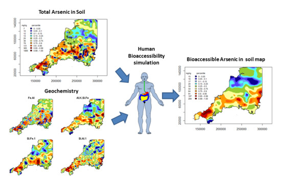
:The aim of this research is to use the whole soil geochemistry and selected bioaccessibility measurements, using the BioAcessibility Research Group of Europe (BARGE) method, on the same soils to identify the geochemical controls on arsenic (As) bioaccessibility and to gain an understanding of its spatial distribution in south-west England. The total element concentrations of 1154 soils were measured with As concentrations ranging from 4.7–1948 mg·kg−1, with the bioaccessible As of 50 selected soils ranging from 0.6–237 mg·kg−1. A Self Modelling Mixture Resolution approach was applied to the total soil element chemistry to identify the intrinsic soil constituents (ISCs). The ISCs were used as predictor variables and As bioaccessibility as the dependant variables in a regression model for the prediction of As bioaccessibility at all soil locations to examine its regional spatial distribution. This study has shown that bioaccessibility measurements can be directly linked to the geochemical properties of soils. In summary, it seems the primary source of bioaccessible As comes from soils developed directly over the mineralised areas surrounding the granite intrusions. Secondary sources of bioaccessible As are derived from As that has been mobilised from the primary mineralised source and then re-absorbed onto clay material, Fe oxides and carbonate coatings. This information can be of direct use for land development, since land contamination can affect the health of people living, working, visiting or otherwise present on a site.
1. Introduction
The geology and mineral deposits of south-west England are diverse [1]. A recent review of the geology [2] as a result of a geochemical survey of stream sediments identifies 16 geological domains (Figure 1) with five major granites playing an important role in the formation of mineralised zones where mining operations have been located. Exploitation of mineral deposits containing economically attractive (Cu, Pb, Zn, Sn, Au, Ag etc.) elements and some that are considered to be harmful, such as As and Pb [3,4] have been undertaken since the Roman era peaking in the mid-nineteenth century. For example, the Devon Great Consols Copper (Cu) and Arsenic (As) mine in the Tamar valley produced over 70, 000 t of As between 1848 and 1909 [5]. The presence of such mineral deposits influences the geochemical nature of the overlying ground (soil) rendering areas considered to be contaminated; this can be exacerbated by extraction during mining activities.
Over the last century geochemical surveys of land masses have been used to identify sites for mineral exploration and more recently provide a useful indicator of areas of soil contamination, e.g., from the presence of elements of interest and subsequent extraction and smelting activities (e.g., [6,7,8,9,10]. Measurement of soil geochemistry provides a snapshot of chemical elements (hazardous and beneficial) in the surface environment at a given point in time (e.g., the time of sampling) [11]. Geochemical soil surveys have been carried out across the world as part of national [12] and continental surveys, e.g., [13], on regional and urban scales (e.g., [14,15,16,17,18,19] and for different land uses (e.g., agricultural soils [20,21]). The detailed geochemical information that they provide highlights the spatial distribution of elements [22] and a reference point by which, for example, environmental change may be monitored and previous land activities identified (e.g., mineral exploration) [17,23]. The usefulness of baseline geochemistry data to health was highlighted in 1998 [24], and more recently, soil geochemistry from baseline data sets has been used to make linkages with the potential hazards to human [25,26,27,28] and animal health [29].
The south-west of England has a population of ca. 5 million accounting for about 8.5 per cent of the UK population [30] and is a popular tourist destination with around 500,000 visitors a year. Through daily activities, both residents and tourists alike will interact with the natural environment and be exposed to soil and any potentially harmful elements (PHE) within. Humans, particularly children as the most vulnerable in society, are exposed to soil PHE by oral, inhalation and dermal pathways. Ingestion is the primary exposure route with an estimated ingested mass of up to 100 mg per day for children [31] and 50 mg per day for adults [32]. Measures of exposure to soil PHEs are made by in vitro (laboratory based) simulation of the human gastro-intestinal (ingestion) pathway [32]. The fraction of PHE that is soluble in this environment is classed as bioaccessible [33] and has the potential to cause harm. The past two decades have seen the development, comparison, refinement and validation of laboratory based bioaccessibility methods for soil contamination. The priority contaminants As and Pb have been the main focus of interest to workers across the world, along with evaluations of PHE availability in a range of soils types and contamination scenarios e.g., [33,34,35,36,37,38,39,40,41]. Performance validation studies, rather than comparison between in vivo (animal) and in vitro (laboratory simulation) data for the same soils [33], have been undertaken, focussing on assessing agreement of model predictions using independent data sets [42].
Over recent years, approaches to provide an understanding of the sources of soil PHE bioaccessibility, as a supporting line of evidence to assess potential mobility, has been to marry in vitro testing with soil sequential extractions [43,44,45,46,47,48,49,50,51,52,53]. These bioaccessibility related studies have widened the range of PHE from those considered to be a priority for human health risk assessment (As, Cd and Pb) to, elements such as chromium (Cr), copper (Cu), cobalt (Co), zinc (Zn), nickel (Ni), vanadium (V) and manganese (Mn), e.g., [54,55]. This combined approach has also been used to understand the effect of aging on PHE mobility [56,57] and the modification of soil physico-chemical properties to reduce PHE toxicity [58,59,60,61].
To predict PHE bioaccessibility over different spatial scales, rather than for soil type or contamination scenarios, soil geochemical data (along with bioaccessibility data) for urban and regional environments have been incorporated into regression modelling [62,63]. Similarly, studies of spatial variation in bioaccessible soil PHE concentrations have been used to assist in the identification of contaminant sources [25,64,65], the main factors controlling contaminant bioaccessibility [66,67] and map hazard quotients for human health risk from soil contaminants [68]. However, there is little work available that spatially predicts and maps PHE bioaccessibility on a regional or urban scale [69].
In this study, the total element concentrations of 1154 soils from south-west England were measured along with the bioaccessibility of As in 50 selected soils (details are given in the Methods section). The aim of this research is twofold:
- (i)
- To use the whole soil geochemistry data and selected bioaccessibility measurements on the same soils to identify the geochemical controls on As bioaccessibility;
- (ii)
- To use regression modelling, with derived data from the whole soil geochemistry as predictor variables and As bioaccessibility as the dependant variables and to predict As bioaccessibility at all soil locations to examine its regional spatial distribution.
2. Materials and Methods
The British Geological Survey’s (BGS), geochemical baseline mapping programme (GBASE) began in the late 1960s using the geochemical mapping methods and techniques established by Professor Jane Plant [17]. The geochemical soil survey of south-west England [70] was completed in 2014, with the collection and preparation (drying and sieving to <2 mm) of 1154 shallow soils (5–20 cm) (Figure 2). The soils were collected at varying densities (ranging from one per 2 km2 to one per 5 km2, depending on underlying parent material homogeneity). Each sample was collected at a depth of 5–20 cm and made up of a composite of material from auger flights taken from five holes distributed within an area of approximately 20 m × 20 m [71]. The survey of south-west England also included high resolution sampling of the Tamar catchment in 2002 [72], shown by the more densely sampled area in Figure 2.
X-Ray Fluorescence Spectrometry (XRFS) was used to determine the elemental content (Ag, Al, As, Ba, Bi, Br, Ca, Cd, Ce, Cl, Co, Cr, Cs, Cu, Fe, Ga, Ge, Hf, I, In, K, La, Mg, Mn, Mo, Na, Nb, Nd, Ni, P, Pb, Rb, S, Sb, Sc, Se, Si, Sm, Sn, Sr, Ta, Te, Th, Ti, Tl, U, V, W, Y, Yb, Zn, Zr) of each soil sample [73]. Details of the reference material quality assurance data obtained whilst running the soil samples is given in the supplementary information (Table S1) along with the XRFS detection limits (Table S2)
Subsamples of 50 representative samples from the 1154 soils were selected for bioaccessibility testing. The selection was carried out using clustering of the samples based on their elemental data measured by XRFS. The geochemistry data set was mean centred and scaled to unit variance and hierarchical clustering was conducted using Euclidean distance and Wards method. Nine clusters were found to be a parsimonious representation of the different variation in geochemistry over the region and represented the underlying geology (Figure 1). Between 5 and 6 samples were randomly chosen from each group to make up 50 samples for bioaccessibility testing. The identified samples, covering a range of As concentrations, were sieved to <250 µm (the size fraction considered to adhere to children’s hands [74,75,76]). The total As concentration of the 50 subsamples (<250 µm) was determined by digestion of 0.25 g in a mixture of nitric, perchloric and hydrofluoric acids followed by inductively coupled plasma mass spectrometery (ICP-MS) analysis [77,78]. Five of the <250 µm sub-samples were digested and analysed in duplicate along with the reference materials NIST 2711a and BGS 102. The digestion repeatability (RSD) was <5% and the extraction recovery of NIST 2711a and BGS 102 was 100% ± 10%. A plot of the location of the samples selected for bioaccessibility testing and an interpolated plot of the total XRFS measured As from the 1154 samples is shown in Figure 2 and Figure 3 respectively.
Bioaccessibility testing using the two stage (stomach and intestine) BioAcessibility Research Group of Europe (BARGE) Unified Bioaccessibility Method (UBM) [33,79] was carried out on the 50 subsamples (<250 µm). As part of the extraction procedure 8 samples were extracted in duplicate along with 8 samples of the guidance material BGS 102. The repeatability of duplicate samples was <10% for all As measurements. The measured As and Pb bioaccessibility in BGS 102 was within reported guidance values [41,69,80].
A Self Modelling Mixture Resolution (SMMR) approach [69] was applied to the total soil element chemistry to identify the intrinsic soil constituents (ISCs) of south-west England (Figure 4) using the Matlab © programming language. An ISC is an assemblage of soil particles from a common biogenic, geogenic or anthropogenic input, with a consistent chemical composition present at varying concentrations in a number of similarly developed soils [81].
Application of the SMMR algorithm to the multi-element XRFS data set resulted in the identification of 22 ISCs for the south-west of England (using the Akaike Information Criterion [82,83]. The SMMR algorithm gives the chemical composition of each ISC and the proportion of each ISC in each sample. The ISCs are named using a combination of the chemical symbols of the elements that make up more than 10% of the ISC. Using a combination of the chemical composition and the spatial distribution of each ISC it is possible to tentatively identify the source of specific ISCs. An example of this for the south-west is given in the Supplementary Information (Figures S1 and S2).
The statistical analysis was carried out using the R programming language [84]. Spatial interpolation and visualisation of the total As, the ISCs associated with bioaccessible As and the predicted bioaccessible As were carried out using the Thin Plate Spline regression (TPS) as implemented in the “fields” package in R [85].
3. Results
3.1. Total As Concentrations
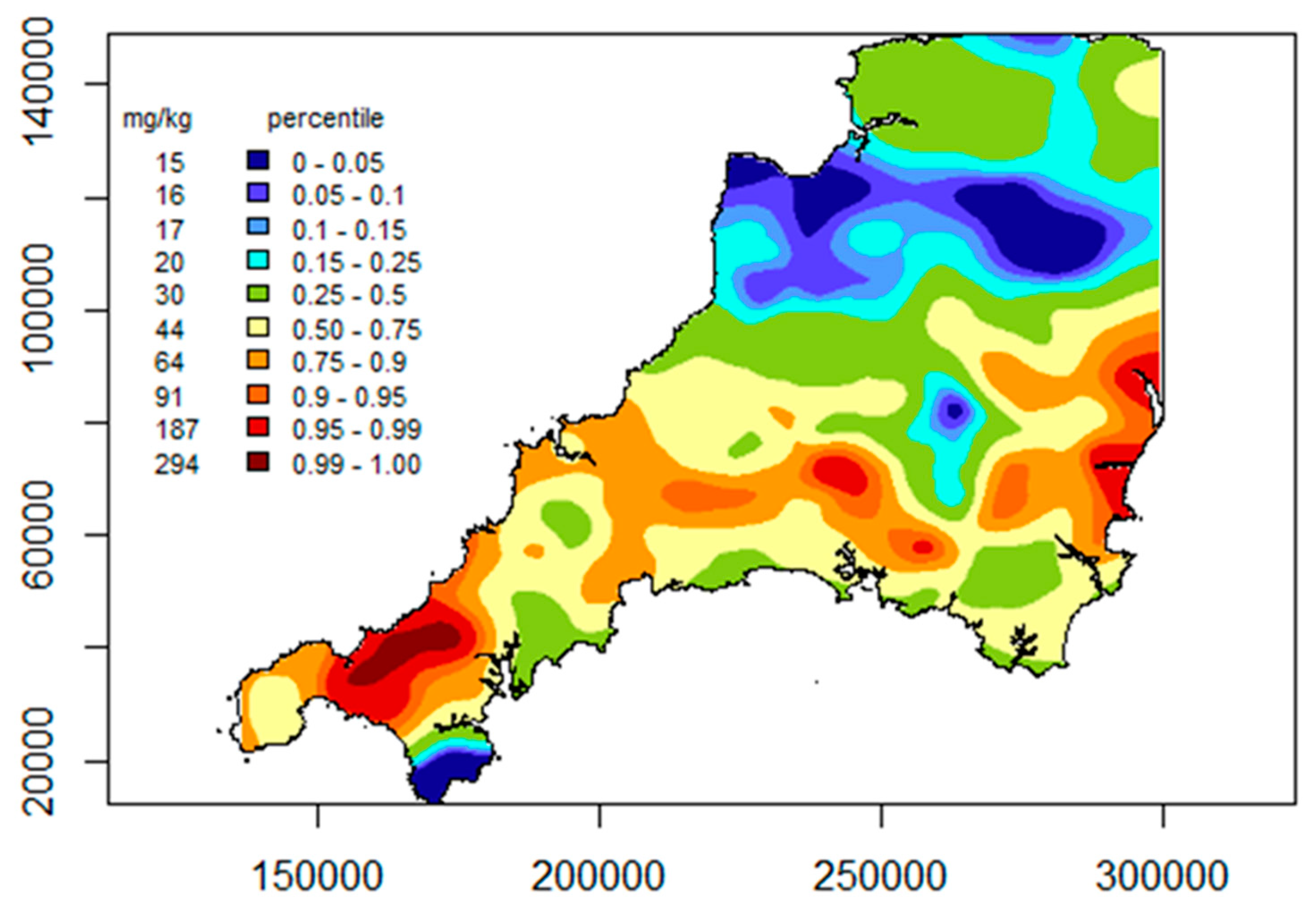
The range of total As concentrations (mg·kg−1) for this study, as measured by XRFS is shown as an interpolated map in Figure 3. Summary statistics for As in the whole data set and the selected samples are shown in Table 1.
The median and the MAD (median absolute deviation) for all three data sets are similar but skew values larger than 1 indicate large positive tails on the data distributions which is why the mean values are significantly larger than the medians. Although a Wilcoxon signed rank test (used to test equality of non-normally distributed data [86]) shows a significant difference between the selected sample XRFS data and the digest data, a linear regression of the digest data on the XRFS data gives a slope not significantly different from 1 and intercept not significantly different from 0 with an r-square of 0.987. Figure 5 shows comparative combined box and whisker plots and violin plots, with the former showing the medians and interquartile ranges and the latter providing a visualisation of the data density. Figure 6 provides information on the relationship between total and bioaccessible As. The summary data in Table 1 and the data distribution plots in Figure 7 suggest that the 50 samples selected for bioaccessibility testing are representative of the larger data set.
Table 2 shows a comparison of measured As against generic assessment criteria and that 25–32% of samples were above the guideline value for residential land uses. When compared to Normal Background Concentrations (NBC) information [87] 35.4–38% of the total As concentration was greater than the principal domain NBC and 2.17–8% above the mineralised domain.
Comparison of mean total As concentrations measured by XRFS in the <2 mm for all of the GBASE samples (n = 1154) and the subset of 50 samples identified for further bioaccessibility testing (XRFS and acid digestion) were compared to both generic assessment criteria (Category 4 Screening Level (C4SL)) and Normal Background Concentrations (NBC), shown in Table 2.
3.2. Bioaccessible As Concentrations
The bioaccessible As concentration in the soil represents the amount of As that would become solubilised in the human gastrointestinal tract and be available for absorption into the systemic circulation [32]. Whilst this is a conservative estimate of the true bioavailable concentration i.e., the actual amount of As absorbed into systemic circulation, it is a much more realistic concentration than the total As concentration in the soil for the purposes of human health risk assessment. The bioaccessible fraction (BAF) is the amount bioaccessible As expressed as a percentage of the total As in the soil. Whilst this is a useful measurement of the relative mobility of the As in a particular soil, it does not provide any information on the absolute magnitude of total or bioaccessible As.
The summary statistics of the bioaccessible As in the stomach and intestine are given in Table 1. A Wilcoxon signed rank test shows that there is a significant difference between the stomach and intestinal phases. A linear regression of intestine against stomach As yields an intercept not significantly different from 0, a slope of 0.85 ± 0.1 and an r-square of 0.987 suggesting that on average the intestinal As concentration is 85% of the stomach As. Table 2 shows that a far smaller percentage of the bioaccessible As values exceed the NBC and C4SL screening levels.
Figure 6A shows the relationship between total As in the <250 µm fraction and the As in the stomach phase, displaying a gradual increase in bioaccessible As between total As values of 0–200 mg·kg−1 followed by a steep rise in bioaccessible As above 200 mg·kg−1. Figure 6B shows that below 200 mg·kg−1 As there is a relatively linear relationship between total and bioaccessible As, with on average 17% of the total As being bioaccessible, although the data become more scattered at total As values of more than 50 mg·kg−1.
Figure 7 shows that there is no correlation between the bioaccessible fraction (BAF) and the total As in the <250 µm fraction (Spearman correlation <0.01). Most of the samples have BAF values between 4% and 16% but there are five samples with BAF values higher than 20%. This shows that, from the consideration of the As data alone, we conclude that there is no simple relationship between the bioaccessible As fraction and the total As present in the soil and that BAF values are not consistent across different concentration ranges (Figure 7). The absolute bioaccessible concentration is therefore a much better measure for comparison of As mobility between sites particularly where there is a high variation in total As concentrations from site to site. In order to get a better understanding of the controls on the bioaccessible As in these soils we need to consider how the overall geochemical make-up of the soils affects As mobility.
4. Discussion
4.1. Intrinsic Soil Constituents
Whilst it is possible to use the individual element concentrations in the soils as possible predictors of bioaccessible As, each individual element will be distributed across different physico-chemical components of the soils, e.g., minerals, mineral coatings, clay, organic matter. As already explained the ISC data represents these soil components and for this reason we preferred to use the ISC data, derived from the total element data, as it would provide a better link to the individual physico-chemical components of the soils.
The SMMR algorithm used to calculate the ISCs also allows us to calculate the proportion of total As summed over all samples associated with each ISC. This provides information on the solid phase fractionation of As in soils from south-west England, which is summarised in an ordered barplot in (Figure 8). We are now interested in how much of the As associated in these ISCs is bioaccessible.
4.2. Regression Modelling of Bioaccessible As
An efficient way of modelling the data and selecting which ISCs, if any, control the bioaccessible As is the “lasso” linear regression algorithm as implemented in the “glmnet” package in the R programming language [88]. Lasso regression shrinks large regression coefficients in order to reduce overfitting, and performs covariate selection by forcing the sum of the absolute value of the regression coefficients to be less than a fixed value, which shrinks certain coefficients to zero, effectively choosing a simpler model that does not include those coefficients.
The masses of each ISC in each sample were used as the predictor variables. Figure 6A shows that the bioaccessible As has a nonlinear response to total As and the summary statistics for bioaccessible As in Table 1 show that the data is right skewed. For this reason we have used a log10 transform of the stomach phase bioaccessible As as the dependant variable. A lasso regularised regression was then carried out selecting the optimum tuning parameter λ by cross validation [88]. The glmnet lasso model was validated with a 10 fold cross validation which gives rise to a cross validated mean square error of 0.0318 log10 bioaccessible As which is equivalent to 1.08 mg·kg−1 bioaccessible As. Figure 9A shows a plot of the predicted vs measured bioaccessible As. Figure 9B shows a bar plot of the ISCs that were selected by the lasso model and the magnitude of coefficient (since all predictor ISCs were mean centred and scaled prior to modelling) gives an approximate measure of the importance of the selected ISCS in predicting bioaccessible As.
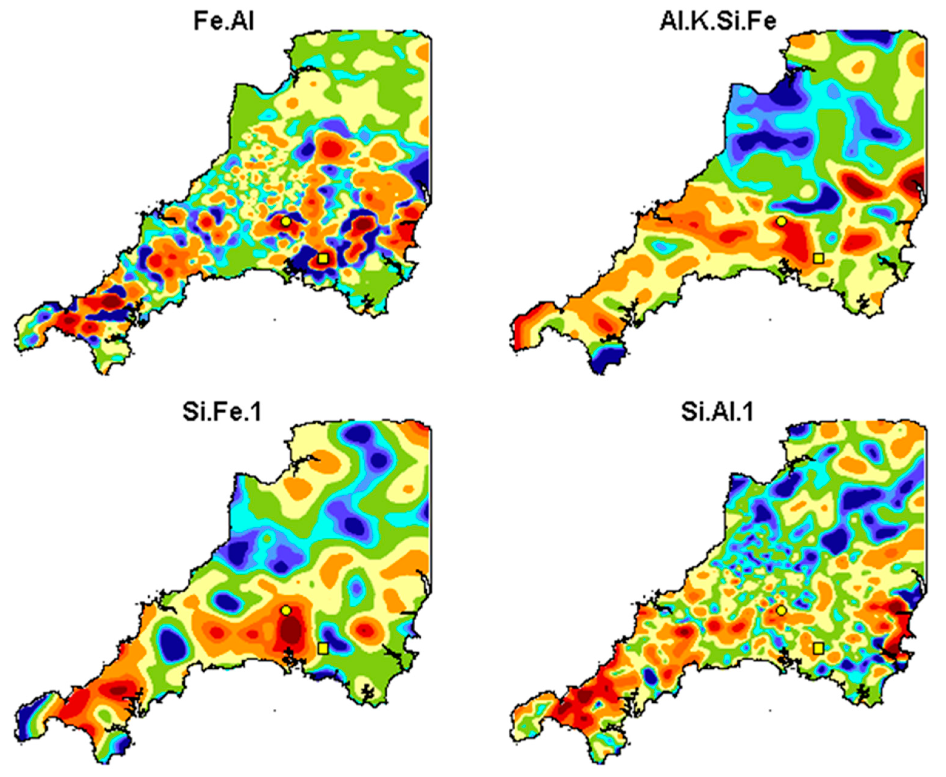
In a classical linear regression the p-value for each coefficient tests the null hypothesis that the coefficient is equal to zero (no effect). A low p-value (<0.05) indicates that you can reject the null hypothesis. In other words, a predictor that has a low p-value is likely to be a meaningful addition to your model because changes in the predictor’s value are related to changes in the response variable. In a lasso regularised regression, the classical p-value cannot be applied. However, estimates of the p-values for this work [89] were obtained by bootstrapping the residuals of the lasso regression 1000 times and counting the number of times out of the 1000 realisations that a particular ISC predictor was given a zero coefficient (i.e., not selected for the model). Using this method, (Figure 10) only four of the ISC coefficients had p-values <0.05 these being Fe.Al, Al.K.Si.Fe, Si.Fe.1 and Si.Al.1. All four are in the top seven total As containing ISCS with the Fe.Al ISC containing the most As (Figure 8). Using the interpolated spatial distribution (Figure 11) and chemical composition of these four ISCs (See Supplementary Material Figures S3–S6) we can make tentative assignments of the source of these components and discuss why their As content contributes to the bioaccessible content of the soils.
Fe.Al: This ISC has the highest concentration of total As associated with it and has the third largest coefficient in the lasso prediction model. The composition plot (Figure S3) shows that it is made principally of Fe (ca. 50%) and Al (ca. 40%) with a low Si (<2%) content. This suggests that this is probably a mixed Fe/Al oxide. It also contains a high concentration of As (ca. 2%) as well as ca. 0.5–1% of Sn, Cu, W which are all elements associated with mining in the south-west of England [90]. The interpolated spatial distribution (Figure 11) shows high areas in the mineralised zones surrounding the granite intrusions (Figure 1), with hotspots (Figure 11) surrounding known mining sites (e.g., Devon Great Consols and Hemerdon mines [90]). This suggests that this ISC is derived from in situ weathering of mineralised rock material and mine spoil.
Al.K.Si.Fe: This ISC has the 4th highest concentration of total As associated with it and has the largest coefficient in the lasso prediction model. The composition plot (Figure S4) shows that it is made principally of Al (ca. 30%), K (ca. 30%) and Fe (ca. 15%) with a Si content that is not well defined. It also contains ca. 0.3% Rb and 0.03% As. The high content of K and Rb suggest that this ISC is a clay related geochemical component. The spatial distribution of this component (Figure 11) shows that it less localised to the mineralised area around the granite intrusions, suggesting that the As content of this component is derived from As mobilised from the high concentration mineralised rock/soil material (possibly by reductive dissolution [91]) which has then been re-absorbed onto soil clay minerals [92].
Si.Fe.1: The Si.Fe.1 ISC has the 3rd highest concentration of total As and the 5th highest coefficient in the lasso prediction model. The composition plot (Figure S5) shows that the Si content is not well defined (it has a very large uncertainty) with an Fe content of ca. 30–70% suggesting that this is an Fe oxide dominated component with ca.0.3% As and high concentrations of other metals (Pb 1%, Cu and Zn 0.5%). Like the Al.K.Si.Fe ISC, the Si.Fe.1 is not localised to the mineralised areas (Figure 11) suggesting that it is secondary Fe oxide component that has adsorbed previously mobilised As arising from the mineralised rock/soil.
Si.Al.1: The Si.Fe.1 ISC has the 7th highest concentration of total As and the 2nd highest coefficients in the lasso prediction model. The composition plot (Figure S6) shows that it is probably a silica dominated component with a Si composition of ca. 40–70%. The presence of relatively high concentrations of Ca and Mg (ca. 7% and ca. 1.5% respectively) suggests carbonate is present as a coating on or within the silicate matrix. The bioaccessible As in this component can be explained by studies [93] which show carbonate in groundwater can release As from Fe oxides into solution which is then precipitated as As enriched carbonates.
4.3. Bioaccessible Arsenic Prediction
Having used the regression model to provide information on the geochemical soil properties controlling As bioaccessibility the model (based on the 50 selected samples) can be used to make predictions of the bioaccessible As at all 1154 sampling locations which can be interpolated and mapped (Figure 12). The As bioaccessibility data for all sampling locations was predicted using the lasso regression model (see the regression modelling section) and the interpolation was carried out by Thin Plate Spline regression (TPS) as implemented in the “fields” package [85] in a similar manner to that used to the total As in soil map shown in Figure 3. This shows a very similar spatial distribution to the total soil As (Figure 3) which is not surprising since the main source of both total As and bioaccessible As is from the mineralised areas around the granite intrusions which relates directly to the Fe.Al ISC (Figure 11) and contains the highest proportion of the total As summed over all samples (Figure 8).
It must be emphasised that the bioaccessible map is only a first order approximation since:
- (i)
- The regression model only looks at linear relationships and does not take into account interaction effects;
- (ii)
- The regression model does not take into account spatial correlation;
- (iii)
- The thin plate spline is not a full spatial model which takes into account the actual spatial variability in the data (e.g., as measured by a variogram [94]);
- (iv)
- No attempts have been made to quantify the overall uncertainty in the predicted values.
Further studies will be required to address these issues when considering the production of a hazard map for As bioaccessibility in soil where accuracy of magnitude and spatial location will be required to delineate areas which are likely to exceed screening guidelines (Table 2).
5. Conclusions
This study has shown that bioaccessibility measurements can be directly linked to the geochemical properties of soils and, by taking a regional view, gain an understanding of the main processes controlling the bioaccessibility and the magnitude of bioaccessible soil As concentration in soils from south-west England. In summary, it seems the primary source of bioaccessible As comes from soils developed directly over the mineralised areas surrounding the granite intrusions. Secondary sources of bioaccessible As are derived from As that has been mobilised from the primary mineralised source and then re-absorbed onto clay material, Fe oxides and carbonate coatings. This information can be of direct use for land development, since land contamination can affect the health of people living, working, visiting or otherwise present on a site. The range of bioaccessible As concentrations found provides an important input parameter to the risk assessment process which is used to establish whether there is an unacceptable risk to humans. As well as the overall magnitude of the bioaccessible As, the information on chemical form can also be useful for evaluating how land use may affect the mobility of As. For example if land use practices provide reducing soil conditions As can be mobilised from Fe oxides [91] and if the pH of the soil is lowered it could liberate As from carbonate coatings.
In addition to the information on the magnitude and mobility of As in soil, this study provides a template for spatial prediction of bioaccessible element concentrations from geochemical soil surveys where it is not feasible to measure the bioaccessibility on every sample by:
- (i)
- Taking a representative selection of soil samples, based on their geochemistry, from the total geochemical survey;
- (ii)
- Measuring the bioaccessibility for the element(s) under study in the selected samples using a robust, validated and well documented method [79];
- (iii)
- Establishing a predictive relationship between the bioaccessible element concentration and the total geochemical composition of the soil using a suitable modelling method;
- (iv)
- Predicting the bioaccessible element concentration for all of the soil samples;
- (v)
- Spatially modelling or interpolating the predicted bioaccessible element concentrations over the region covered by the geochemical soil survey.
Further work is required to refine the spatial modelling process to take into account non-linearity, interaction effects, spatial correlation and prediction uncertainty.
Supplementary Materials
The following is available online at https://www.mdpi.com/2075-163X/8/12/570/s1, a word document containing: an example ISC from south west England data (Figures S1 and S2); plots of the four geochemical components which contribute to the bioaccessible As content of the soils in Figures S3–S6; and quality assurance data for XRFS analysis of soils consisting of reference material data and detection limit information in Tables S1 and S2.
Author Contributions
J.W. and M.C designed the project; T.R.L. was responsible for overseeing the soil sampling and the XRFS analysis and associated data quality assurance; E.H. undertook the bioaccessibility testing; M.C. carried out the statistical analysis and modelling; J.W. wrote the initial draft of the paper which was further modified by J.W. and M.C. after further discussions with all the authors.
Funding
This research received no external funding.
Acknowledgments
We thank the student volunteer workers who collected the GBASE samples used in this study. This paper is published with the permission of the Executive Director of the BGS.
Conflicts of Interest
The authors declare no conflict of interest. The funders had no role in the design of the study; in the collection, analyses, or interpretation of data; in the writing of the manuscript, or in the decision to publish the results.
References
- Dines, H.G. The Metalliferous Mining Region of South-West England, 1st ed.; HMSO: London, UK, 1956.
- Kirkwood, C.; Everett, P.; Ferreira, A.; Lister, B. Stream sediment geochemistry as a tool for enhancing geological understanding: An overview of new data from south west England. J. Geochem. Explor. 2016, 163, 28–40. [Google Scholar] [CrossRef] [Green Version]
- ATSDR. Toxicological Profile for Lead; Agency for Toxic Substances and Disease Registry: Atlanta, GA, USA, 2007.
- ATSDR. Toxicological Profile for Arsenic; Agency for Toxic Substances and Disease Registry: Atlanta, GA, USA, 2007.
- Palumbo-Roe, B.; Klinck, B. Bioaccessibility of arsenic in mine waste-contaminated soils: A case study from an abandoned arsenic mine in SW England (UK). J. Environ. Sci. Health Part A Toxic Hazard. Subst. Environ. Eng. 2007, 42, 1251–1261. [Google Scholar] [CrossRef] [PubMed] [Green Version]
- Ghasemi, A.; Manesh, S.M.T.; Tabatabaei, S.H.; Mokhtari, A.R. Geoenvironmental studies and heavy metal mapping in soil: The case of Ghohroud area, Iran. Environ. Earth Sci. 2015, 74, 5221–5232. [Google Scholar] [CrossRef]
- González-Corrochano, B.; Esbrí, J.; Alonso-Azcárate, J.; Martínez-Coronado, A.; Jurado, V.; Higueras, P. Environmental geochemistry of a highly polluted area: The La Union Pb–Zn mine (Castilla-La Mancha region, Spain). J. Geochem. Explor. 2014, 144, 345–354. [Google Scholar] [CrossRef]
- Kasimov, N.; Kosheleva, N.; Gunin, P.; Korlyakov, I.; Sorokina, O.; Timofeev, I. State of the environment of urban and mining areas in the Selenga Transboundary River Basin (Mongolia Russia). Environ. Earth Sci. 2016, 75, 1283. [Google Scholar] [CrossRef]
- Khorasanipour, M.; Esmaeilzadeh, E. Environmental characterization of Sarcheshmeh Cu-smelting slag, Kerman, Iran: Application of geochemistry, mineralogy and single extraction methods. J. Geochem. Explor. 2016, 166, 1–17. [Google Scholar] [CrossRef]
- Levitan, D.M.; Zipper, C.E.; Donovan, P.; Schreiber, M.E.; Seal, R.R.; Engle, M.A.; Chermak, J.A.; Bodnar, R.J.; Johnson, D.K.; Aylor, J.G. Statistical analysis of soil geochemical data to identify pathfinders associated with mineral deposits: An example from the Coles Hill uranium deposit, Virginia, USA. J. Geochem. Explor. 2015, 154, 238–251. [Google Scholar] [CrossRef]
- Salminen, R.; Gregorauskiene, V. Considerations regarding the definition of a geochemical baseline of elements in the surficial materials in areas differing in basic geology. Appl. Geochem. 2000, 15, 647–653. [Google Scholar] [CrossRef]
- Salminen, R.; Tarvainen, T. The problem of defining geochemical baselines. A case study of selected elements and geological materials in Finland. J. Geochem. Explor. 1997, 60, 91–98. [Google Scholar] [CrossRef]
- Caritat, P.; Reimann, C.; Team, N.P.; Team, G.P. Comparing results from two continental geochemical surveys to world soil composition and deriving Predicted Empirical Global Soil (PEGS2) reference values. Earth Planet. Sci. Lett. 2012, 319, 269–276. [Google Scholar] [CrossRef]
- Fordyce, F.M.; Brown, S.E.; Ander, E.L.; Rawlins, B.G.; O’Donnell, K.E.; Lister, T.R.; Breward, N.; Johnson, C.C. GSUE: Urban geochemical mapping in Great Britain. Geochemistry 2005, 5, 325–336. [Google Scholar] [CrossRef]
- Galan, E.; Fernandez-Caliani, J.C.; Gonzalez, I.; Aparicio, P.; Romero, A. Influence of geological setting on geochemical baselines of trace elements in soils. Application to soils of South-West Spain. J. Geochem. Explor. 2008, 98, 89–106. [Google Scholar] [CrossRef]
- Glennon, M.; Harris, P.; Ottesen, R.; Scanlon, R.; O’connor, P. The Dublin SURGE Project: Geochemical baseline for heavy metals in topsoils and spatial correlation with historical industry in Dublin, Ireland. Environ. Geochem. Health 2014, 36, 235–254. [Google Scholar] [CrossRef] [PubMed]
- Johnson, C.C.; Ander, E.L. Urban geochemical mapping studies: How and why we do them. Environ. Geochem. Health 2008, 30, 511–530. [Google Scholar] [CrossRef] [PubMed] [Green Version]
- Ludden, J.; Peach, D.; Flight, D. Geochemically based solutions for urban society: London, a case study. Elements 2015, 11, 253–258. [Google Scholar] [CrossRef]
- Sierra, M.; Martinez, F.J.; Aguilar, J. Baselines for trace elements and evaluation of environmental risk in soils of Almeria (SE Spain). Geoderma 2007, 139, 209–219. [Google Scholar] [CrossRef]
- Reimann, C.; Birke, M.; Demetriades, A.; Filzmoser, P.; O’Connor, P. Chemistry of Europe’s Agricultural Soils—Part B: General Background Information and Further Analysis of the GEMAS Data Set; E. Schweizerbart Science Publishers: Stuttgart, Germany, 2014. [Google Scholar]
- Reimann, C.; Birke, M.; Demetriades, A.; Filzmoser, P.; O’Connor, P. Chemistry of Europe’s Agricultural Soils, Part A. Environ. Earth Sci. 2014, 72, 3239–3242. [Google Scholar]
- Garrett, R.G. Relative spatial soil geochemical variability along two transects across the United States and Canada. Appl. Geochem. 2009, 24, 1405–1415. [Google Scholar] [CrossRef]
- Eze, P.N.; Knight, J.; Evans, M. Tracing recent environmental changes and pedogenesis using geochemistry and micromorphology of alluvial soils, Sabie-Sand River Basin, South Africa. Geomorphology 2016, 268, 312–321. [Google Scholar] [CrossRef]
- Plant, J.; Baldock, J.; Haslam, H.; Smith, B. The role of geochemistry in environmental and epidemiological studies in developing countries. Episodes 1998, 21, 19–27. [Google Scholar] [CrossRef]
- Gamino-Gutierrez, S.P.; Gonzalez-Perez, C.I.; Gonsebatt, M.E.; Monroy-Fernandez, M.G. Arsenic and lead contamination in urban soils of Villa de la Paz (Mexico) affected by historical mine wastes and its effect on children’s health studied by micronucleated exfoliated cells assay. Environ. Geochem. Health 2013, 35, 37–51. [Google Scholar] [CrossRef]
- Hooker, P.J.; Nathanail, C.P. Risk-based characterisation of lead in urban soils. Chem. Geol. 2006, 226, 340–351. [Google Scholar] [CrossRef]
- Morrison, S.; Fordyce, F.; Scott, E.M. An initial assessment of spatial relationships between respiratory cases, soil metal content, air quality and deprivation indicators in Glasgow, Scotland, UK: Relevance to the environmental justice agenda. Environ. Geochem. Health 2014, 36, 319–332. [Google Scholar] [CrossRef] [PubMed] [Green Version]
- Smyth, D.; Johnson, C.C. Distribution of iodine in soils of Northern Ireland. Geochemistry 2011, 11, 25. [Google Scholar] [CrossRef]
- Wylie, C.; Shaw, D.; Fordyce, F.; Lilly, A.; McGorum, B. Equine grass sickness in S cotland: A case–control study of signalment-and meteorology-related risk factors. Equine Vet. J. 2014, 46, 64–71. [Google Scholar] [CrossRef] [PubMed] [Green Version]
- Smith, E. Portrait of the South West. Reg. Trends 2010, 42, 43–59. [Google Scholar] [CrossRef] [Green Version]
- Calabrese, E.J.; Stanek, E.J.; Barnes, R. Soil ingestion rates in children identified by parental observation as likely high soil ingesters. J. Soil Contam. 1997, 6, 271–279. [Google Scholar] [CrossRef]
- Swartjes, A. Dealing with Contaminated Sites: From Theory towards Practical Application; Springer: London, UK, 2011. [Google Scholar]
- Denys, S.; Caboche, J.; Tack, K.; Rychen, G.; Wragg, J.; Cave, M.; Jondreville, C.; Feidt, C. In Vivo Validation of the Unified BARGE Method to Assess the Bioaccessibility of Arsenic, Antimony, Cadmium, and Lead in Soils. Environ. Sci. Technol. 2012, 46, 6252–6260. [Google Scholar] [CrossRef] [PubMed] [Green Version]
- Basta, N.T.; Scheckel, K.G.; Bradham, K.D.; Richey, J.S.; Dayton, E.A.; Whitacre, S.W.; Casteel, S.W. Soil Chemical Controls on Arsenic Bioaccessibility and Bioavailability. Epidemiology 2008, 19, S29. [Google Scholar]
- Juhasz, A.L.; Weber, J.; Smith, E. Impact of soil particle size and bioaccessibility on children and adult lead exposure in pen-urban contaminated soils. J. Hazard. Mater. 2011, 186, 1870–1879. [Google Scholar] [CrossRef]
- Juhasz, A.L.; Weber, J.; Smith, E.; Naidu, R.; Marschner, B.; Rees, M.; Rofe, A.; Kuchel, T.; Sansom, L. Evaluation of SBRC-Gastric and SBRC-Intestinal Methods for the Prediction of In Vivo Relative Lead Bioavailability in Contaminated Soils. Environ. Sci. Technol. 2009, 43, 4503–4509. [Google Scholar] [CrossRef] [PubMed]
- Li, J.; Li, K.; Cave, M.; Li, H.-B.; Ma, L.Q. Lead bioaccessibility in 12 contaminated soils from China: Correlation to lead relative bioavailability and lead in different fractions. J. Hazard. Mater. 2015, 295, 55–62. [Google Scholar] [CrossRef] [PubMed] [Green Version]
- Lowney, Y.W.; Ruby, M.V.; Salatas, J.; Pastorok, R. The relative bioavailability of metals from soil to ecological receptors. Toxicol. Sci. 2003, 72, 398–399. [Google Scholar]
- Oomen, A.G.; Hack, A.; Minekus, M.; Zeijdner, E.; Cornelis, C.; Schoeters, G.; Verstraete, W.; Van de Wiele, T.; Wragg, J.; Rompelberg, C.J.M.; et al. Comparison of five in vitro digestion models to study the bioaccessibility of soil contaminants. Environ. Sci. Technol. 2002, 36, 3326–3334. [Google Scholar] [CrossRef] [PubMed]
- Van de Wiele, T.R.; Oomen, A.G.; Wragg, J.; Cave, M.; Minekus, M.; Hack, A.; Cornelis, C.; Rompelberg, C.J.M.; De Zwart, L.L.; Klinck, B.; et al. Comparison of five in vitro digestion models to in vivo experimental results: Lead bioaccessibility in the human gastrointestinal tract. J. Environ. Sci. Health. Part A 2007, 42, 1203–1211. [Google Scholar] [CrossRef] [PubMed] [Green Version]
- Wragg, J.; Cave, M.; Basta, N.; Brandon, E.; Casteel, S.; Denys, S.; Gron, C.; Oomen, A.; Reimer, K.; Tack, K.; et al. An inter-laboratory trial of the unified BARGE bioaccessibility method for arsenic, cadmium and lead in soil. Sci. Total Environ. 2011, 409, 4016–4030. [Google Scholar] [CrossRef] [PubMed] [Green Version]
- Basta, N.T.; Juhasz, A. Using In Vivo Bioavailability and/or In Vitro Gastrointestinal Bioaccessibility Testing to Adjust Human Exposure to Arsenic from Soil Ingestion. In Arsenic: Environmental Geochemistry, Mineralogy, and Microbiology, Proceedings of the 24th Annual V.M. Goldschmidt Conference and held at the Miners Foundry, Nevada City, CA, USA, 15–16 June 2014; Bowell, R.J., Alpers, C.N., Jamieson, H.E., Nordstrom, D.K., Majzlan, J., Eds.; Mineralogical Society of America: Chantilly, VA, USA, 2014; Volume 79, pp. 451–472. [Google Scholar]
- Cave, M.; Wragg, J.; Gowing, C.; Gardner, A. Measuring the solid-phase fractionation of lead in urban and rural soils using a combination of geochemical survey data and chemical extractions. Environ. Geochem. Health 2015, 37, 779–790. [Google Scholar] [CrossRef] [PubMed] [Green Version]
- Cox, S.; Chelliah, M.M.; McKinley, J.; Palmer, S.; Ofterdinger, U.; Young, M.; Cave, M.; Wragg, J. The importance of solid-phase distribution on the oral bioaccessibility of Ni and Cr in soils overlying Palaeogene basalt lavas, Northern Ireland. Environ. Geochem. Health 2013, 35, 553–567. [Google Scholar] [CrossRef] [Green Version]
- Karadas, C.; Kara, D. Chemometric evaluation for the relation of BCR sequential extraction method and in vitro gastro-intestinal method for the assessment of metal bioavailability in contaminated soils in Turkey. Environ. Sci. Pollut. Res. 2012, 19, 1280–1295. [Google Scholar] [CrossRef]
- Li, S.W.; Li, J.; Li, H.B.; Naidu, R.; Ma, L.Q. Arsenic bioaccessibility in contaminated soils: Coupling in vitro assays with sequential and HNO3 extraction. J. Hazard. Mater. 2015, 295, 145–152. [Google Scholar] [CrossRef]
- Luo, X.S.; Yu, S.; Li, X.D. The mobility, bioavailability, and human bioaccessibility of trace metals in urban soils of Hong Kong. Appl. Geochem. 2012, 27, 995–1004. [Google Scholar] [CrossRef]
- Palumbo-Roe, B.; Wragg, J.; Cave, M. Linking selective chemical extraction of iron oxyhydroxides to arsenic bioaccessibility in soil. Environ. Pollut. 2015, 207, 256–265. [Google Scholar] [CrossRef] [PubMed] [Green Version]
- Patinha, C.; Reis, A.P.; Dias, C.; Cachada, A.; Adao, R.; Martins, H.; da Silva, E.F.; Sousa, A.J. Lead availability in soils from Portugal’s Centre Region with special reference to bioaccessibility. Environ. Geochem. Health 2012, 34, 213–227. [Google Scholar] [CrossRef] [PubMed]
- Pelfrene, A.; Waterlot, C.; Mazzuca, M.; Nisse, C.; Bidar, G.; Douay, F. Assessing Cd, Pb, Zn human bioaccessibility in smelter-contaminated agricultural topsoils (northern France). Environ. Geochem. Health 2011, 33, 477–493. [Google Scholar] [CrossRef] [PubMed]
- Reis, A.P.; Patinha, C.; Wragg, J.; Dias, A.C.; Cave, M.; Sousa, A.J.; Costa, C.; Cachada, A.; da Silva, E.F.; Rocha, F.; et al. Geochemistry, mineralogy, solid-phase fractionation and oral bioaccessibility of lead in urban soils of Lisbon. Environ. Geochem. Health 2014, 36, 867–881. [Google Scholar] [CrossRef] [PubMed] [Green Version]
- Witt, E.C., III; Shi, H.; Wronkiewicz, D.J.; Pavlowsky, R.T. Phase partitioning and bioaccessibility of Pb in suspended dust from unsurfaced roads in Missouri—A potential tool for determining mitigation response. Atmos. Environ. 2014, 88, 90–98. [Google Scholar] [CrossRef]
- Wragg, J.; Cave, M.R. Assessment of a geochemical extraction procedure to determine the solid phase fractionation and bioaccessibility of potentially harmful elements in soils: A case study using the NIST 2710 reference soil. Anal. Chim. Acta 2012, 722, 43–54. [Google Scholar] [CrossRef]
- Kelepertzis, E.; Stathopoulou, E. Availability of geogenic heavy metals in soils of Thiva town (central Greece). Environ. Monit. Assess. 2013, 185, 9603–9618. [Google Scholar] [CrossRef]
- Pascaud, G.; Leveque, T.; Soubrand, M.; Boussen, S.; Joussein, E.; Dumat, C. Environmental and health risk assessment of Pb, Zn, As and Sb in soccer field soils and sediments from mine tailings: Solid speciation and bioaccessibility. Environ. Sci. Pollut. Res. 2014, 21, 4254–4264. [Google Scholar] [CrossRef]
- Huang, G.; Chen, Z.; Zhang, Y.; Liu, F.; Wang, J.; Hou, Q. Changes of arsenic fractionation and bioaccessibility in wastewater-irrigated soils as a function of aging: Influence of redox condition and arsenic load. Geoderma 2016, 280, 1–7. [Google Scholar] [CrossRef]
- Huang, Y.Z.; Hao, X.W. Effect of red mud addition on the fractionation and bio-accessibility of Pb, Zn and As in combined contaminated soil. Chem. Ecol. 2012, 28, 37–48. [Google Scholar] [CrossRef]
- Im, J.; Yang, K.; Jho, E.H.; Nam, K. Effect of different soil washing solutions on bioavailability of residual arsenic in soils and soil properties. Chemosphere 2015, 138, 253–258. [Google Scholar] [CrossRef] [PubMed]
- Jelusic, M.; Lestan, D. Effect of EDTA washing of metal polluted garden soils. Part I: Toxicity hazards and impact on soil properties. Sci. Total Environ. 2014, 475, 132–141. [Google Scholar] [CrossRef] [PubMed]
- Reijonen, I.; Metzler, M.; Hartikainen, H. Impact of soil pH and organic matter on the chemical bioavailability of vanadium species: The underlying basis for risk assessment. Environ. Pollut. 2016, 210, 371–379. [Google Scholar] [CrossRef] [PubMed]
- Zagury, G.J.; Bello, J.A.R.; Guney, M. Valorization of a treated soil via amendments: Fractionation and oral bioaccessibility of Cu, Ni, Pb, and Zn. Environ. Monit. Assess. 2016, 188, 222. [Google Scholar] [CrossRef]
- Appleton, J.D.; Cave, M.R.; Palumbo-Roe, B.; Wragg, J. Lead bioaccessibility in topsoils from lead mineralisation and urban domains, UK. Environ. Pollut. 2013, 178, 278–287. [Google Scholar] [CrossRef] [Green Version]
- Malone, B.P.; Jha, S.K.; Minasny, B.; McBratney, A.B. Comparing regression-based digital soil mapping and multiple-point geostatistics for the spatial extrapolation of soil data. Geoderma 2016, 262, 243–253. [Google Scholar] [CrossRef]
- Jean-Soro, L.; Le Guern, C.; Bechet, B.; Lebeau, T.; Ringeard, M.F. Origin of trace elements in an urban garden in Nantes, France. J. Soils Sediments 2015, 15, 1802–1812. [Google Scholar] [CrossRef]
- Percival, J.B.; White, H.P.; Goodwin, T.A.; Parsons, M.B.; Smith, P.K. Mineralogy and spectral reflectance of soils and tailings from historical gold mines, Nova Scotia. Geochem. Explor. Environ. Anal. 2014, 14, 3–16. [Google Scholar] [CrossRef]
- Palmer, S.; Ofterdinger, U.; McKinley, J.M.; Cox, S.; Barsby, A. Correlation analysis as a tool to investigate the bioaccessibility of nickel, vanadium and zinc in Northern Ireland soils. Environ. Geochem. Health 2013, 35, 569–584. [Google Scholar] [CrossRef] [Green Version]
- Zhu, X.; Yang, F.; Wei, C. Factors influencing the heavy metal bioaccessibility in soils were site dependent from different geographical locations. Environ. Sci. Pollut. Res. 2015, 22, 13939–13949. [Google Scholar] [CrossRef] [PubMed] [Green Version]
- Pelfrene, A.; Detriche, S.; Douay, F. Combining spatial distribution with oral bioaccessibility of metals in smelter-impacted soils: Implications for human health risk assessment. Environ. Geochem. Health 2015, 37, 49–62. [Google Scholar] [CrossRef] [PubMed]
- Cave, M.R.; Wragg, J.; Harrison, H. Measurement modelling and mapping of arsenic bioaccessibility in Northampton, UK. J.Environ. Sci. Health Part A 2013, 48, 629–640. [Google Scholar] [CrossRef] [PubMed]
- British Geological Survey, G-BASE for South West England. Available online: http://www.bgs.ac.uk/gbase/gBaseSW.html (accessed on 18 October 2018).
- Flight, D.M.A.; Scheib, A.J. Soil Geochemical Baselines in UK Urban centres: The G-BASE Project. In Mapping the Chemical Environment of Urban Areas; Johnson, C., Demetriades, A., Locutura, J., Ottesen, R.T., Eds.; Wiley-Blackwell: Oxford, UK, 2011; pp. 186–206. [Google Scholar]
- Rawlins, B.; O’Donnell, K.; Ingham, M. Geochemical Survey of the Tamar Catchment (South-West England); CR/03/027; British Geological Survey: Nottingham, UK, 2003. [Google Scholar]
- Johnson, C.C.; Breward, N.; Ander, E.L.; Ault, L. G-BASE: Baseline geochemical mapping of Great Britain and Northern Ireland. Geochemistry 2005, 5, 347–357. [Google Scholar] [CrossRef]
- Qin, J.H.; Nworie, O.E.; Lin, C.X. Particle size effects on bioaccessible amounts of ingestible soil-borne toxic elements. Chemosphere 2016, 159, 442–448. [Google Scholar] [CrossRef] [PubMed] [Green Version]
- Duggan, M.J.; Inskip, M.J.; Rundle, S.A.; Moorcroft, J.S. Lead in Playground Dust and on the Hands of Schoolchildren. Sci. Total Environ. 1985, 44, 65–79. [Google Scholar] [CrossRef]
- USEPA. Test Methods for Evaluating Solid Waste; SW-846; U.S. Environmental Protection Agency: Washington, DC, USA, 2000.
- Middleton, D.R.; Watts, M.J.; Beriro, D.J.; Hamilton, E.M.; Leonardi, G.S.; Fletcher, T.; Close, R.M.; Polya, D.A. Arsenic in residential soil and household dust in Cornwall, South West England: Potential human exposure and the influence of historical mining. Environ. Sci. 2017, 19, 517–527. [Google Scholar] [CrossRef]
- Watts, M.J.; Button, M.; Brewer, T.S.; Jenkin, G.R.; Harrington, C.F. Quantitative arsenic speciation in two species of earthworms from a former mine site. J. Environ. Monit. 2008, 10, 753–759. [Google Scholar] [CrossRef]
- ISO. Assessment of human exposure from ingestion of soil. In Soil Quality; ISO: Geneva, Switzerland, 2018. [Google Scholar]
- Appleton, J.D.; Cave, M.R.; Wragg, J. Anthropogenic and geogenic impacts on arsenic bioaccessibility in UK topsoils. Sci. Total Environ. 2012, 435, 21–29. [Google Scholar] [CrossRef] [Green Version]
- Wragg, J.; Cave, M.; Nathanail, P. A Study of the relationship between arsenic bioaccessibility and its solid-phase distribution in soils from Wellingborough, UK. J. Environ. Sci. Health. Part A 2007, 42, 1303–1315. [Google Scholar] [CrossRef]
- Akaike, H. A new look at the statistical model identification. IEEE Trans. Autom. Control 1974, 19, 716–723. [Google Scholar] [CrossRef]
- Schwarz, G. Estimating the dimension of a model. Ann. Stat. 1978, 6, 461–464. [Google Scholar] [CrossRef]
- R Core Team. R: A Language and Environment for Statistical Computing; R Foundation for Statistical Computing: Vienna, Austria, 2017. [Google Scholar]
- Nychka, D.; Furrer, R.; Paige, J.; Sain, S. Fields: Tools for Spatial Data; R Foundation for Statistical Computing: Vienna, Austria, 2017. [Google Scholar]
- Bauer, D.F. Constructing Confidence Sets Using Rank Statistics. J. Am. Stat. Assoc. 1972, 67, 687–690. [Google Scholar] [CrossRef]
- Ander, E.L.; Johnson, C.C.; Cave, M.R.; Palumbo-Roe, B.; Nathanail, C.P.; Lark, R.M. Methodology for the determination of normal background concentrations of contaminants in English soil. Sci. Total Environ. 2013, 454–455, 604–618. [Google Scholar] [CrossRef] [PubMed]
- Friedman, J.; Hastie, T.; Tibshirani, R. Regularization Paths for Generalized Linear Models via Coordinate Descent. J. Stat. Softw. 2010, 33, 1–22. [Google Scholar] [CrossRef]
- Hastie, T.; Tibshirani, R.; Wainwright, M. Statistical Learning with Sparsity: The Lasso and Generalizations; CRC Press: Boca Raton, FL, USA, 2015. [Google Scholar]
- Rollin, K.; Gunn, A.; Scrivener, R.; Shaw, M. Potential for Stratiform Massive Sulphide Mineralisation in South-West England; British Geological Survey: Nottingham, UK, 2001. [Google Scholar]
- Cornell, R.M.; Schwertmann, U. The Iron Oxides—Structure Properties, Reactions, Occurences and Uses; VCH Publishers: Weinheim, Germany, 1996. [Google Scholar]
- Ghorbanzadeh, N.; Jung, W.; Halajnia, A.; Lakzian, A.; Kabra, A.N.; Jeon, B.-H. Removal of arsenate and arsenite from aqueous solution by adsorption on clay minerals. Geosyst. Eng. 2015, 18, 302–311. [Google Scholar] [CrossRef]
- Appelo, C.A.J.; Van Der Weiden, M.J.J.; Tournassat, C.; Charlet, L. Surface Complexation of Ferrous Iron and Carbonate on Ferrihydrite and the Mobilization of Arsenic. Environ. Sci. Technol. 2002, 36, 3096–3103. [Google Scholar] [CrossRef]
- Rawlins, B.G.; Lark, R.M.; O’Donnell, K.E.; Tye, A.M.; Lister, T.R. The assessment of point and diffuse metal pollution of soils from an urban geochemical survey of Sheffield, England. Soil Use Manag. 2005, 21, 353–362. [Google Scholar] [CrossRef]
Figure 1.
Geological domains for the south-west of England [2].
Figure 1.
Geological domains for the south-west of England [2].
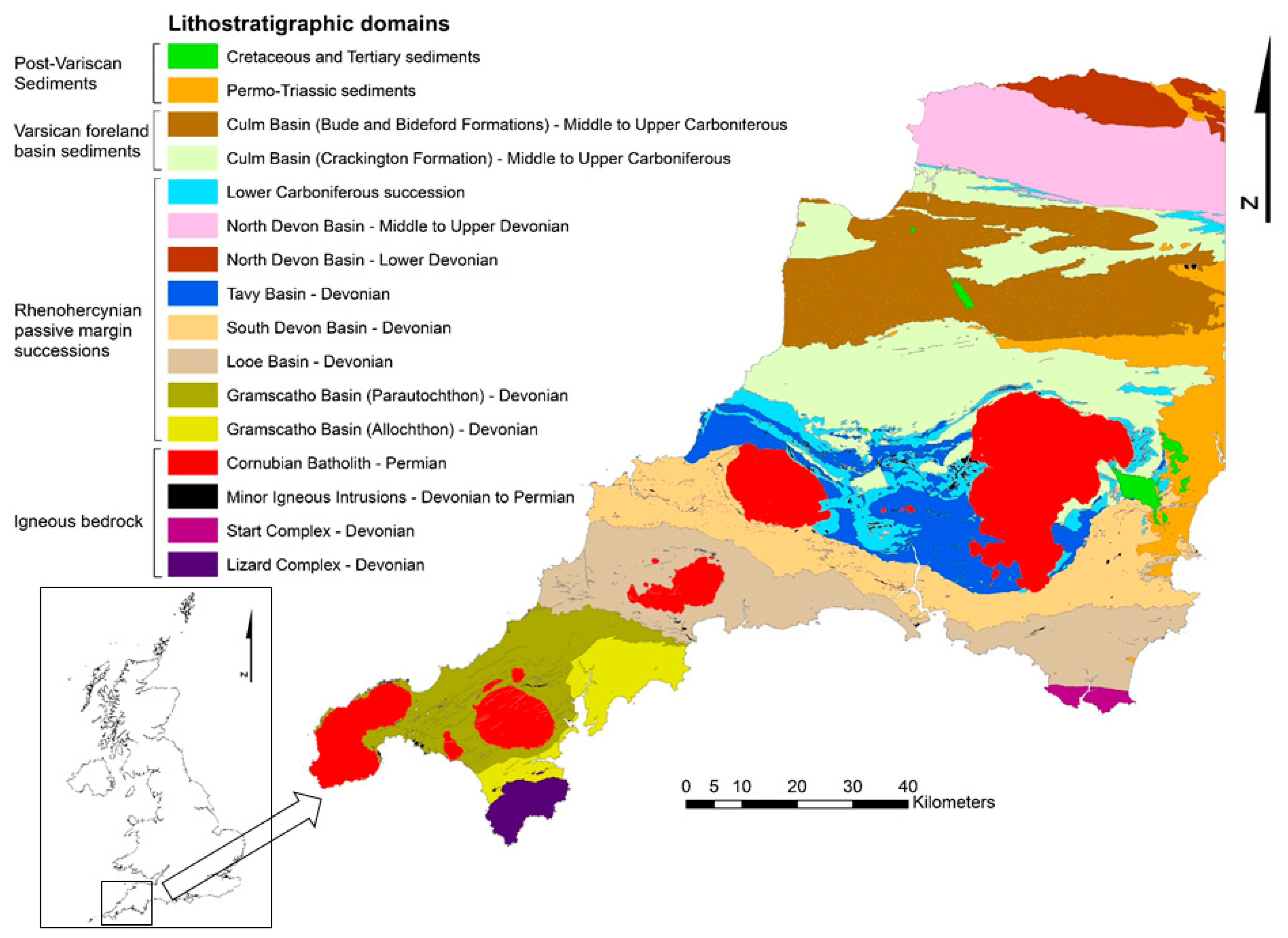
Figure 2.
Sample locations for the geochemical baseline mapping programme (GBASE) south-west England soils.
Figure 2.
Sample locations for the geochemical baseline mapping programme (GBASE) south-west England soils.
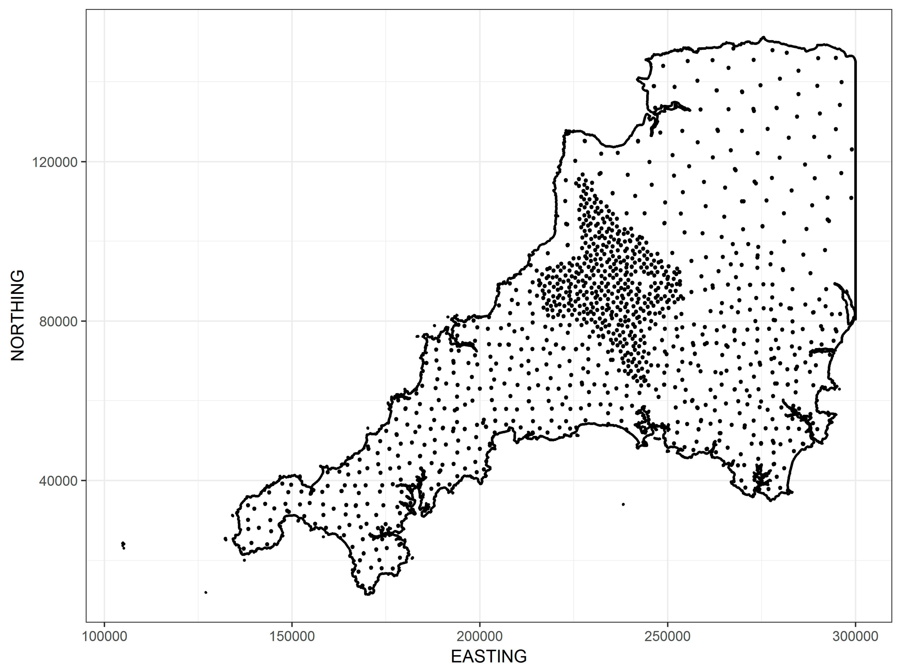
Figure 3.
Interpolated map of total XRFS As in soils in south-west England with locations of the samples chosen for bioaccessibility testing. (x-axis is EASTING, y-axis is NORTHING).
Figure 3.
Interpolated map of total XRFS As in soils in south-west England with locations of the samples chosen for bioaccessibility testing. (x-axis is EASTING, y-axis is NORTHING).

Figure 4.
Representation of the Self Modelling Mixture Resolution (SMMR) algorithm.
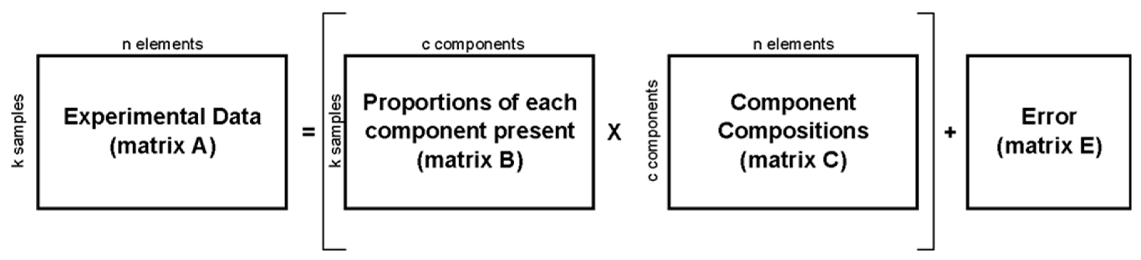
Figure 5.
Combined box and whisker and violin plots of the total As data in the whole data set, the selected samples and the digest analysis of the <250 µm fraction of the selected soils.
Figure 5.
Combined box and whisker and violin plots of the total As data in the whole data set, the selected samples and the digest analysis of the <250 µm fraction of the selected soils.
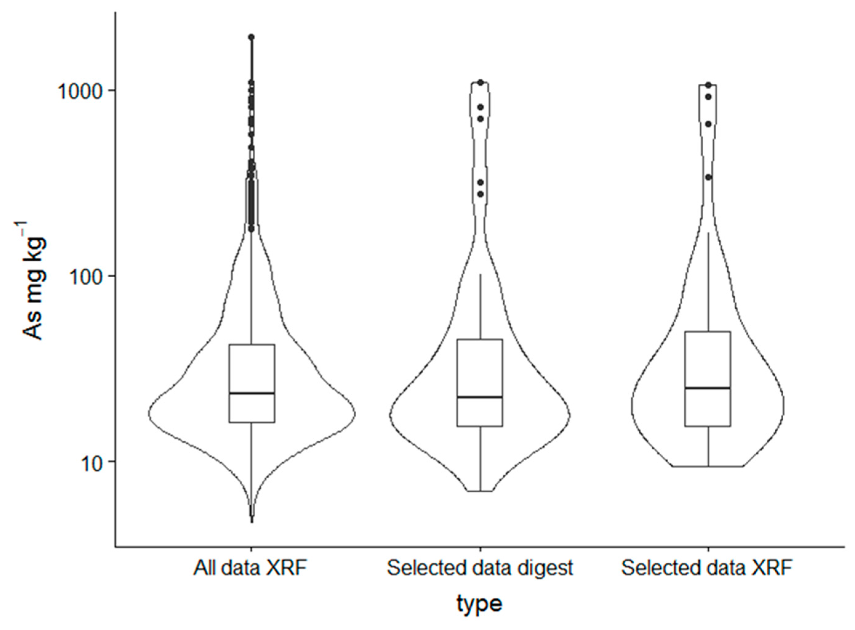
Figure 6.
Relationship between total As in the <250 µm fraction and the bioaccessible stomach phase As. (A) full range of total As with Loess fit line, (B) total As <200 mg·kg−1 with linear regression fit line. Grey region indicates standard error on the fit.
Figure 6.
Relationship between total As in the <250 µm fraction and the bioaccessible stomach phase As. (A) full range of total As with Loess fit line, (B) total As <200 mg·kg−1 with linear regression fit line. Grey region indicates standard error on the fit.
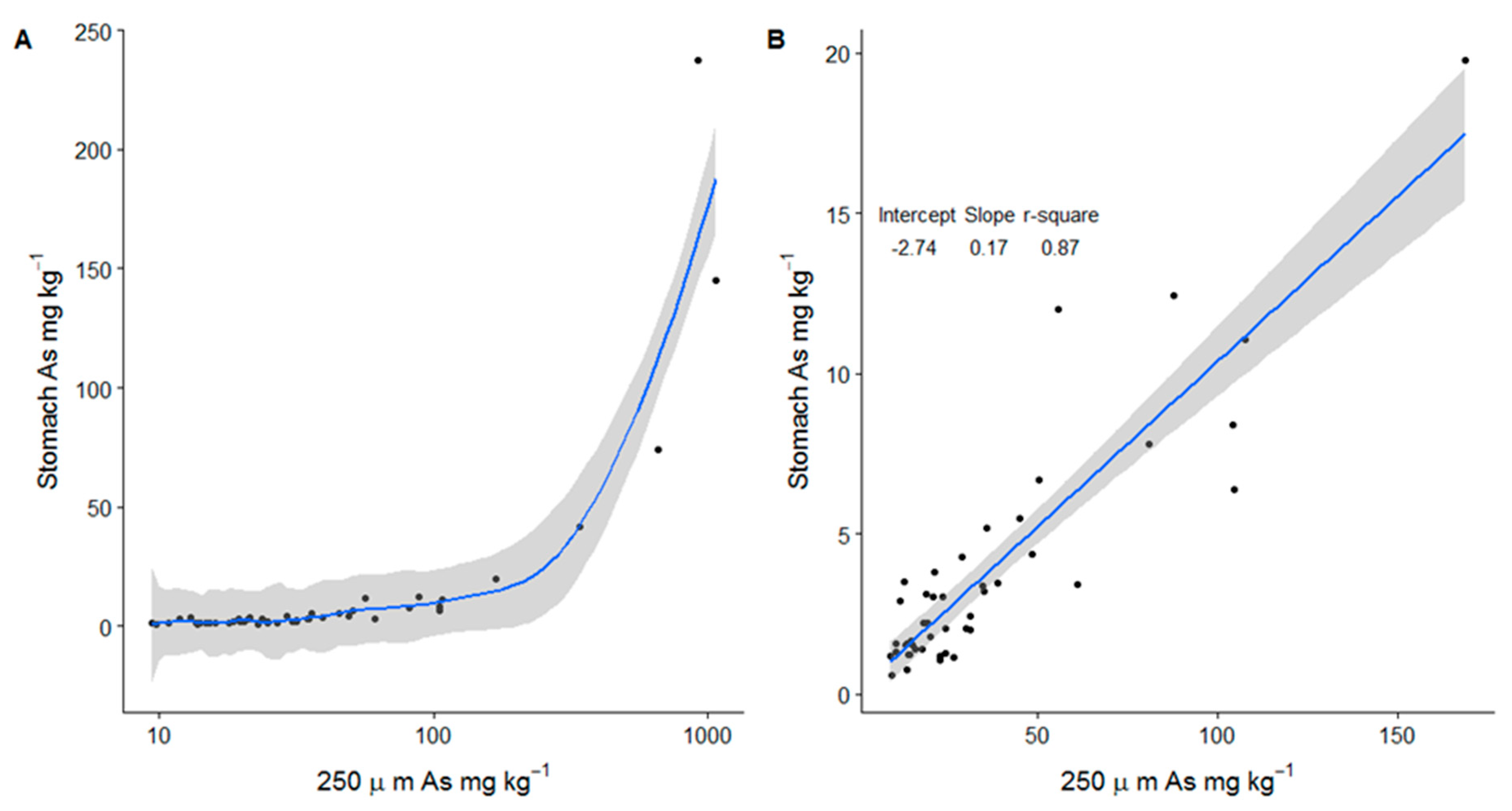
Figure 7.
Relationship between total As in the <250 μm particle size and the bioaccessible As fraction. The histograms on plot show the separate marginal distributions of the bioaccessible As fraction and the total As in the selected soils.
Figure 7.
Relationship between total As in the <250 μm particle size and the bioaccessible As fraction. The histograms on plot show the separate marginal distributions of the bioaccessible As fraction and the total As in the selected soils.
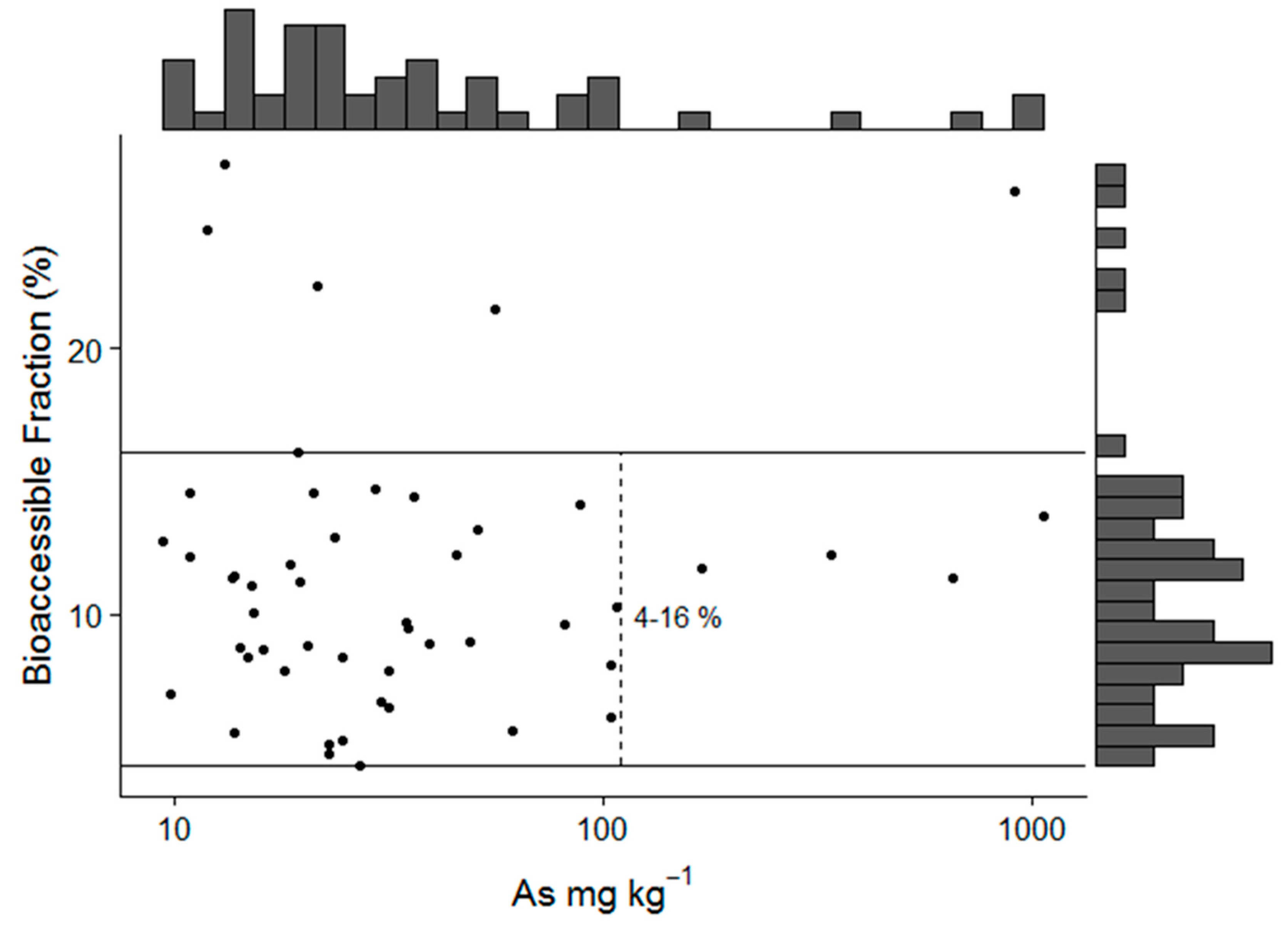
Figure 8.
Solid phase distribution of total As between the soil intrinsic soil constituents (ISCs) in south-west England.
Figure 8.
Solid phase distribution of total As between the soil intrinsic soil constituents (ISCs) in south-west England.
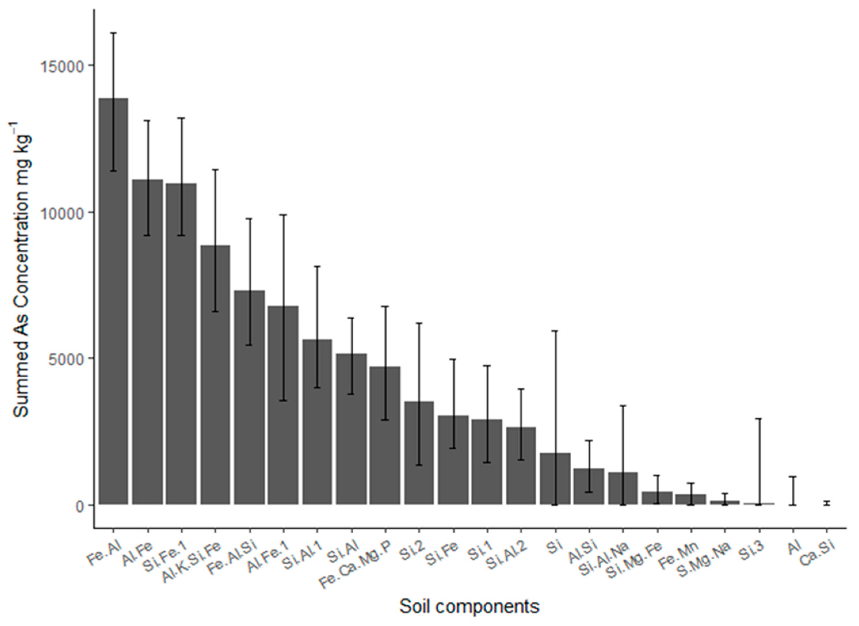
Figure 9.
Lasso regression model data for bioaccessible As (A)—predicted bioaccessible As vs measured bioaccessible As with line of equivalence. (B)—Relative magnitude of lasso chosen ISC coefficients.
Figure 9.
Lasso regression model data for bioaccessible As (A)—predicted bioaccessible As vs measured bioaccessible As with line of equivalence. (B)—Relative magnitude of lasso chosen ISC coefficients.
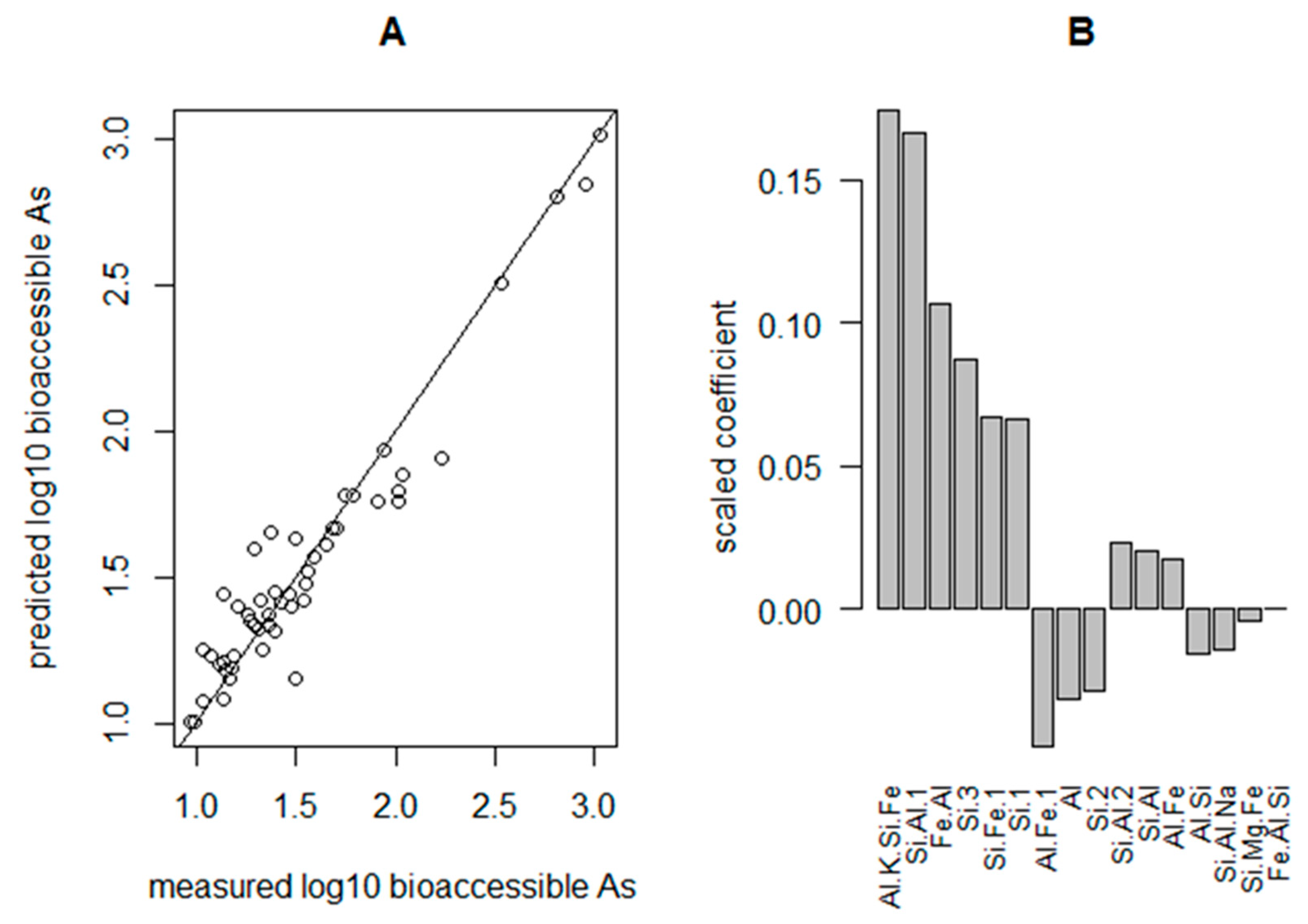
Figure 10.
Bootstrap estimated p-values for the lasso coefficients, dotted line represents a p-value of 0.05.
Figure 10.
Bootstrap estimated p-values for the lasso coefficients, dotted line represents a p-value of 0.05.
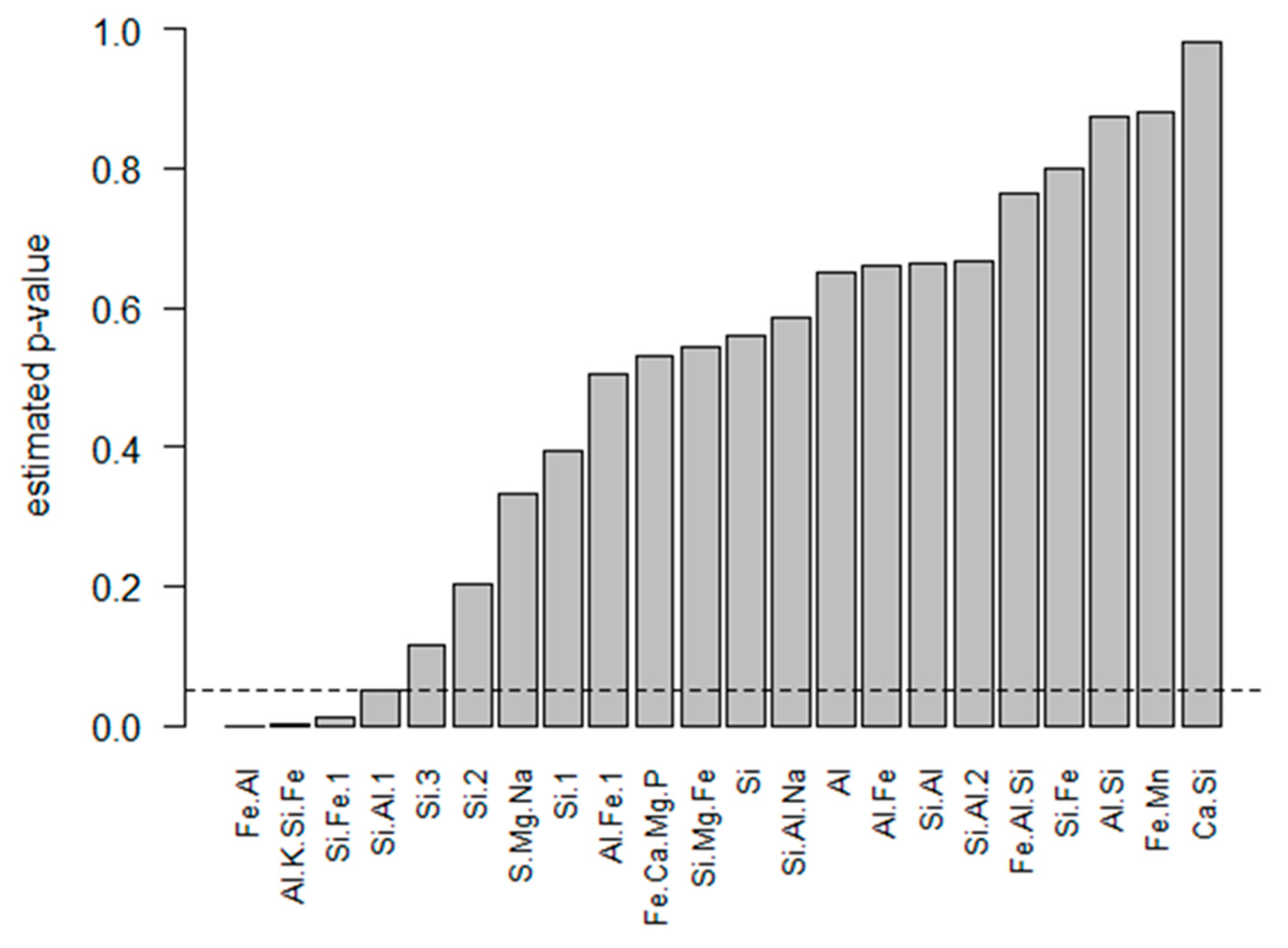
Figure 11.
Relative distributions in deciles of the concentration of the 4 ISCs associated with bioaccessible As. Colours follow percentile gradient in Figure 12. ◯ symbol indicates location of the Devon Great Consols mine and the ◻ symbol indicates the location of the Hemerden mine.
Figure 11.
Relative distributions in deciles of the concentration of the 4 ISCs associated with bioaccessible As. Colours follow percentile gradient in Figure 12. ◯ symbol indicates location of the Devon Great Consols mine and the ◻ symbol indicates the location of the Hemerden mine.

Figure 12.
Interpolated map of predicted bioaccessible As in south- west England.

Table 1.
Summary statistics for As (mg·kg−1) in the entire data set and the selected samples.
| N | Mean | Sd | Median | Mad | Min | Max | Range | Skew | |
|---|---|---|---|---|---|---|---|---|---|
| All data XRF | 1154 | 50.2 | 108 | 23.1 | 13.8 | 4.7 | 1949 | 1945 | 8.9 |
| Selected data digest | 50 | 92.4 | 211 | 24.7 | 16.2 | 9.4 | 1063 | 1053 | 3.5 |
| Selected data XRF | 50 | 91 | 211 | 21.9 | 12.6 | 6.9 | 1102 | 1095 | 3.5 |
| Bioaccessible As (Stomach) | 50 | 13.4 | 39.6 | 3 | 2.3 | 0.6 | 237 | 237 | 4.4 |
| Bioaccessible As (Intestine) | 50 | 11.4 | 33.7 | 2.5 | 2 | 0.7 | 206 | 205 | 4.5 |
Wilcoxon signed rank test between the selected sample XRFS data and the digest data, p value = 0.003.
Table 2.
Comparison of measured As concentrations assessment criteria.
| Sample Type | C4SL (37 mg·kg−1) | NBC Principal (32 mg·kg−1) | NBC Mineralised (290 mg·kg−1) |
|---|---|---|---|
| Number of samples (total As) above criteria <2 mm XRFS (n = 1154) | 340 | 408 | 25 |
| % | 29.5 | 35.4 | 2.17 |
| Number of samples (total As) above criteria <2 mm XRFS (n = 50) | 16 | 18 | 4 |
| % | 32 | 36 | 8 |
| Number of samples (total As) above criteria <250 µm acid digestion (n = 50) | 16 | 19 | 4 |
| % | 32 | 38 | 8 |
| Number of samples (bioaccessible As) above criteria <250 µm acid digestion (n = 50) | 4 | 4 | 0 |
| % | 8 | 8 | 0 |
© 2018 by the authors. Licensee MDPI, Basel, Switzerland. This article is an open access article distributed under the terms and conditions of the Creative Commons Attribution (CC BY) license (http://creativecommons.org/licenses/by/4.0/).
Share and Cite
MDPI and ACS Style
Wragg, J.; Cave, M.; Hamilton, E.; Lister, T.R. The Link between Soil Geochemistry in South-West England and Human Exposure to Soil Arsenic. Minerals 2018, 8, 570. https://doi.org/10.3390/min8120570
AMA Style
Wragg J, Cave M, Hamilton E, Lister TR. The Link between Soil Geochemistry in South-West England and Human Exposure to Soil Arsenic. Minerals. 2018; 8(12):570. https://doi.org/10.3390/min8120570
Chicago/Turabian StyleWragg, Joanna, Mark Cave, Elliott Hamilton, and T. Robert Lister. 2018. "The Link between Soil Geochemistry in South-West England and Human Exposure to Soil Arsenic" Minerals 8, no. 12: 570. https://doi.org/10.3390/min8120570
Note that from the first issue of 2016, this journal uses article numbers instead of page numbers. See further details here.