Article

A Posteriori Analysis of Analytical Models for Heap Leaching Using Uncertainty and Global Sensitivity Analyses

by
Mario E. Mellado
1,†,
Luis A. Cisternas
1,2,*,
Freddy A. Lucay
2,
Edelmira D. Gálvez
1,3 and
Felipe D. Sepúlveda
4
1
Mining Technological and Scientific Research Center (CICITEM), Antofagasta 1240000, Chile
2
Department of Chemical and Mineral Process Engineering, Universidad de Antofagasta, Antofagasta 1240000, Chile
3
Department of Mines and metallurgical engineering, Universidad Católica del Norte, Antofagasta 1240000, Chile
4
Department of Mines Engineering, Universidad de Antofagasta, Antofagasta 1240000, Chile
*
Author to whom correspondence should be addressed.
Requiescat in pace.
Minerals 2018, 8(2), 44; https://doi.org/10.3390/min8020044
Submission received: 30 October 2017 / Revised: 19 January 2018 / Accepted: 23 January 2018 / Published: 26 January 2018
(This article belongs to the Special Issue Heap Leaching: The State-of-the-Art)

Abstract

:
The heap leaching of minerals is one of the more commonly used processes in the mining industry. This process has been modeled by many authors. However, the validation, verification, and implementation of these models are difficult since there is uncertainty about the operating conditions and the leaching model parameters. This work uses the uncertainty quantification, based on uncertainty and sensitivity analysis, for studying the model strength against uncertainties in heap leaching. The uncertainty analysis (UA) is used to quantify the effect of the magnitude of the uncertainties of the input variables on the recovery of heap leaching. Global sensitivity analysis (GSA) is used to study the nature of connections between the recovery and input variables of the leaching model. In addition, GSA facilitates the detection of whether a leaching model is over-parameterized. The information obtained allows studying some applications of the kinetic model. The Mellado et al. kinetic model is used as an example. The UA results indicate that the kinetic model can estimate the recovery behavior considering the full range of uncertainties of input variables. The GSA indicates that the kinetic model is over-parameterized on the uncertainties range considered; this conclusion contradicts the results when the local sensitivity analysis is used. However, the model shows a good correlation between the results of GSA and the kinetic behavior of heap leaching. In addition, the kinetic model presents versatility because it allows the determination of operating regions for heap leaching.

1. Introduction

The hydrometallurgical process of heap leaching is one of the most commonly used processes in the mining industry. Heap leaching allows the processing of low-grade metallic minerals (for example, less than 1% copper) [1,2]; nonmetallic minerals [3,4], and potentially yttrium and heavy rare earth elements [5]. In fact, heap leaching is often the preferred method for extracting metal from low-grade ore deposits as it provides a low capital cost compared to other methods [6]. This low cost is due to the fact that energy-intensive comminution is not required. However, this is contrasted with often slow and inefficient recovery [7,8]. In addition, small changes in metal extraction efficiency drive considerable changes in operating cash flow margins and affect project viability [9]. The performance of heap leaching depends on many input variables (operational and design), i.e., its optimization is complex. A thorough review on heap leaching has been published [10], and one important conclusion is that the long-term success of heap leaching as a technology choice requires a concerted high-level cross-disciplinary engineering approach from research and development to design to construction to operation and to closure.
Heap leaching is a mineral processing technology whereby piles of crushed or agglomerate materials are leached with various chemical solutions that extract valuable minerals [11]. These chemical solutions are a weak sulfuric acid solution for copper, diluted alkaline cyanide solution for gold, and water for nitrate minerals. The valuable-containing minerals are irrigated with the chemical solution which dissolves the valuable metal from the mineral, and the pregnant leach solution (PLS) passes down through the ore pile and is recovered at the base of the heap. The valuable material is extracted from the PLS using different technologies, and the chemical solution is recycled back onto the leach pile. The most common methods for recovery of valuable minerals are solvent extraction and the electro winning processes for copper, crystallization operations for nitrates, and either activated carbon or precipitation with zinc for gold.
In the literature, there is a range of scientific research on modeling and optimizing the leaching process; some examples will be briefly presented. De Andrade Lima [12] reported a model developed to simulate the transient evolution of the dissolved chemical species in the heap and column isothermal leaching processes. Bouffard and Dixon [13] published a study about heap leaching planning considering an optimization approach. Bouffard and Dixon [14] compared the rates of pore diffusion and cyanide gold dissolution in coarse, porous gold oxide ore particles. Cross et al. [15] described a computational model for the analysis of multiphase flows in reactive porous media targeted at metal recovery through stockpile leaching and environmental recovery processes. Sheikhzadeh et al. [16] numerically and experimentally studied an unsaturated flow of liquid in a bed of uniform and spherical ore particles. Galvez et al. [17] performed a computational evaluation of a phenomenological model to optimize the copper leaching. They developed an unsteady and two-dimensional model based on the mass conservation equations of the liquid phase in the bed and the particles. Mellado and Cisternas [18] presented an analytical-numerical scheme for solving the heap leaching problem, but the model still contained mathematical complexities. Bouffard and Dixon [19] reviewed heap leaching of refractory gold ores and analyzed the effect of operating parameters (e.g., flow rate, particle size, height and aeration flow). Bennett et al. [20] and McBride et al. [21] presented a comprehensive copper heap leach model based on computational fluid dynamics together with its parameterization and validation against laboratory column test data and plant data. The modeling of heap leaching also includes soft computing such as an artificial neural network. Hoseinian et al. [22] applied an artificial neural network and a genetic algorithm to predict copper recoveries and determine the optimized conditions of column leaching of a copper ore.
A good model development should include model verification, validation and uncertainty quantification [23]. Model verification is used to ensure that the model is behaving properly. For example, the model can be compared with other models or with known analytical solutions. Model validation is the comparison with experimental data. Uncertainty quantification studies the effect of the uncertainties on the model. Uncertainty and sensitivity analyses can be used to provide a general overview of the effect of the uncertainties.
Several aforementioned studies helped to understand the behavior of leaching systems. However, the model is usually validated based on experimental data, and verification and uncertainty quantification are not considered in the model development. For example, Ordoñez et al. [24,25] performed an experimental validation of a phenomenological model for the leaching of caliche with the aim of assessing their level of mathematical adjustment. However, Liddell [26] indicates that a simple adjustment or comparison with experimental values is not enough to validate a leaching model, especially empirical and hybrid models. Specifically, Liddell [26] reported that a data set of titanium leaching from ilmenite (FeTiO3) could be represented by four shrinking core models (spherical particles under reaction control, spherical particles under layer diffusion control, cylindrical particles under reaction control and cylindrical particles under layer diffusion control).
Mellado et al. [27] developed a model that combined aspects of phenomenology with empirical expression. Their results are comparable to the ones obtained from more complex models. However, the Mellado et al. model considered that the recovery at infinite time is equal to one, which is not observed in practice. Therefore, an expression for the recovery at infinite time was added to the previous model [28]. The Mellado et al. model has been validated in several ways. First, it was used to model the recovery of copper minerals from northern Chile in pilot heaps measuring 3, 6 and 9 m in height, obtaining a determination coefficient of 99.74 [28]. In other words, the Mellado et al. model was able to explain 99.74% of the variability in the recovery. Ding et al. [29] applied the Mellado et al. equations to model the heap leaching of uranium ore. The kinetic model gave the fitting precision of more than 95% and prediction precision of more than 93%. The Mellado et al. model was also verified with the results obtained from a simulation of heaps following the Dixon and Hendrix [30,31] phenomenological model, solved by using an analytic-numerical procedure as proposed in the literature [18]. Different values of particle size and superficial velocity were used to adjust the Mellado et al. model, showing the fit to be very good (0.28% deviation). Then, the model was used for prediction (both interpolation and extrapolation) with very similar results (0.29% deviation). All these studies have been performed on one variable at a time (or one-factor-at-a-time, OAT). OAT has been demonstrated to be inefficient for the study of model sensitivity [32]. Uncertainty quantification has not been applied to the Mellado et al. model.
Saltelli et al. [33] indicated that sensitivity analysis had been claimed to be an essential ingredient in all phases of model building (model identification, model calibration, and model corroboration). Sensitivity analysis allows studying the nature of the connections between the output variables and input variables. Additionally, sensitivity analysis allows identifying if a model is over-parameterized. There are two types of sensitivity analysis: Local sensitivity analysis and global sensitivity analysis (GSA) [34,35]. Local sensitivity analysis has several limitations such as linearity and normality assumptions, as well as local variations. GSA considers the entire range of input variations and does not assume linearity and normality of the input variables.
Sensitivity analysis can be another tool for model development that can be used in addition to verification and experimental validation. Mellado et al. [36] applied a local sensitivity analysis to completely evaluate an analytical heap leaching model, as previously described in the literature [27,28]. Later, these results were used for the optimization of the irrigation flow rate [37]. McBride et al. [21] performed a local sensitivity analysis to validate the computational fluid dynamics model proposed. Local sensitivity analysis had been applied in numerous studies of heap leaching [4,24,31,38]. The most popular local sensitivity analysis practice is that of “one-factor-at-a-time”. This consists of analyzing the effect of varying one model input variable at a time while keeping all others fixed. Although the shortcomings of “one-factor-at-a-time” are known from the statistical literature, it is still widely used. In fact, Salteli [32] introduced geometric proof of the inefficiency of “one-factor-at-a-time”, with the purpose of providing the modeling community with a convincing and possibly definitive argument against “one-factor-at-a-time”. The inadequacy of “one-factor-at-a-time” is not limited to sensitivity analysis (SA), but to uncertainty analysis (UA) as well. The elementary statistics of the model output, for instance, its maximum, or mode, can be misinterpreted via “one-factor-at-a-time”.
This work aims to apply UA and GSA as tools for uncertainty quantification of heap leach models. Specifically, the goals are identification of the key inputs that influence the uncertainty of model recovery, a better understanding of the effects of inputs variables on the output variables, and accomplishing model simplification based on detection of whether the model is over-parameterized.
The paper is organized as follows. Section 2 describes the models and methodologies used. In Section 2.1, the kinetic model studied in this paper is described. In Section 2.2 the uncertainty analysis (UA) is presented. In Section 2.3, a brief description of the GSA is presented, and Section 2.4 presents the regionalizations of variables. In Section 3, the results are given together with the discussion, including UA (Section 3.1), GSA (Section 3.2), and regionalization (Section 3.3). Finally, in Section 4, some conclusions are presented.

2. Analytical Models for Heap Leaching

2.1. Mellado Model

Mellado et al. [27] considered that the behavior of the heap could be modeled using a system of first-order equations such as:
y τ = k τ y n τ
where y is a dynamic quantity, such as the concentration or the recovery ( R t ), k τ is the kinetic constant and n τ is the order of the reaction. The subscript τ represents a time scale that depends on the phenomenon to model. To solve Equation (1), an initial condition is required. Then, Mellado et al. introduced a delay, i.e., a time ω where the R t begins to change ( R t ( ω ) = 0). The general solution to this problem is known (see Mellado et al. [27] for the general solution), for n τ = 1 the solution is:
R τ = R τ ( 1 e k τ ( τ ω ) )
Dixon and Hendrix [30,31] considered that the leaching phenomenon occurs at different scales of size and time, and that different phenomena participate in the leaching process. It is possible to represent these phenomena using Equation (2) with expressions associated with the particle and height of heap leaching. At the particle level, they considered that the phenomenon was dominated by the diffusion of the dissolved products from the mineral particles to the bulk of the leaching solution. Then, they defined a dimensionless diffusion time [30,31]:
τ = D A e t ε o r 2
where D A e is the effective diffusivity of the solute within the particle pores (cm3/cm·s), ε o is the porosity of the particle, t is the time (s), r the particle radius (cm). At the bulk level, Dixon and Hendrix considered that the heap is represented by the porous bulk formed of particles through which the leaching solution flows at a constant rate. Then, they defined the dimensionless time of the bulk [30,31]
θ = u s t ε b Z
where u s is a superficial velocity of lixiviant flow through the bed (cm3/cm·s), ε b is the volumetric fraction of the bulk solution in the bed, and Z is the height of the heap (cm). Then, Equation (2) can be written for both dimensionless times as [27,28]:
R τ = R τ ( 1 e k τ ( D A e ε o r 2 t ω ¯ ) )
R θ = R θ ( 1 e k θ ( u s ε b Z t ω ) )
where ω ¯ represents the delay in the scale of τ. Following the phenomenological model of Dixon and Hendrix [30,31], it is possible to demonstrate that [27]
ω ¯ = D A e ε o r 2 · ε b Z u s · ω
For the inclusion of both scales in the processing of the heap, it was assumed that the total recovery is the sum of the recoveries on both scales, that is R = R τ + R θ . In addition, it was considered that that each recovery has an asymptotic behavior with increasing time, this is R = R τ + R θ . Therefore, the total recovery is:
R = R ( 1 λ e k θ · u s ε b Z ( t ε b Z u s · ω ) ( 1 λ ) e k τ · D A e ε o r 2 ( t ε b Z u s · ω ) )
where λ is defined as the kinetic weight factor. In addition, Mellado et al. [28] developed a mathematical expression for R :
R ( α , β , γ , r , Z ) = α Z γ + β [ 1 ( 1 Z γ + β α ) Z / 2 r ]
This new expression shows that the R is influenced by the radius of the particle ( r ), height of the heap leaching ( Z ) and three coefficients of mathematical adjustment (α, β and γ). When Z r , the expression for R is
R ( α , β , γ , Z ) = α Z γ + β
Finally, the heap leaching model is given by [28]:
R = α Z γ + β ( 1 λ e k θ · u s ε b Z ( t ε b Z u s · ω ) ( 1 λ ) e k τ · D A e ε o r 2 ( t ε b Z u s · ω ) )

2.2. Uncertainty Analysis

The UA corresponds to determining the uncertainty in the output variables as a result of uncertainty in the input variables. The UA is usually done using the probability theory where the uncertainty is represented by probability distribution functions (PDF), but there are other available theories such as the fuzzy theory. In the probability theory, the process is performed in four steps. First, the type of PDF and the magnitude of uncertainty is determined for each input variable; in other words, the input uncertainty is characterized. Then, for each input variable, a sample is generated from the PDF. This process is usually performed using random sampling, but other methods such as Latin hypercube sampling are available when small samples are required. Thirdly, values of the output variables are determined for each element of the sample. If the model is costly, this stage may be demanding regarding computational calculations. Finally, the results are analyzed using graphics, descriptive statistics, and statistical tests to characterize the behavior of the output variables.
As commented before, the uncertainties of input variables can be represented through a PDF. When the input variables have epistemic uncertainties, the uncertainty can be represented by a uniform distribution. Design and operating variables present this type of uncertainty. When input variables have stochastic uncertainties, the normal distribution is usually used to represent this type of uncertainty.

2.3. Sensitivity Analysis

The SA can be defined as the study of how the uncertainty in the output of a model (numerical or otherwise) can be apportioned to different sources of uncertainty in the model input [39]. There are two types of SA: Local sensitivity analysis and GSA. The first quantifies the rate of change of the model output due to small variations in the uncertainties of the input variables. One of the disadvantages of local sensitivity analysis is that the choice of the assessment point could sharply influence the results, especially when the sampling space of the input variables is affected by a considerable uncertainty. However, GSA considers the full range of uncertainties of the input variables represented by PDF.
GSA techniques have been widely used in various engineering areas and are of great importance in determining the most significant variables in a model. The general objectives of GSA are [40,41] (a) the identification of the significant and insignificant input variables and the possible reduction of the dimensions of an optimization problem; (b) the improvement in the understanding of the model behavior (highlighting interactions among factors and finding combinations of factors that result in high or low values for the model output); (c) mapping the output behavior in function of the inputs by focusing on a specific domain of inputs if necessary; and (d) calibrating some model inputs using some available information.
There are several methods to perform the GSA, but among these methods, those based on variance decomposition stand out, due to their versatility and efficiency [42]. Therefore, in this study, we will use such methods, specifically those based on the Sobol method [43]. In variance-based methods, the variance V of a model Y = f ( X 1 , X 2 , , X k ) is fully decomposed into terms depending on the k uncertain input variables and their interactions. The number of interactions increases exponentially with the number of input variables, which is why all interactions are rarely determined. More often practitioners are satisfied with computing just k first order effects ( S i ) and k total effects ( S T i ), the latter describing synthetic interactions among input factors. The first order sensitivity index measures only the main effect contribution of each input variable on the output variance. It does not take into account the interactions among variables. Two factors are said to interact if their total effect on the output is not equal to the sum of their first order effects. A model without interactions is said to be additive. The first order indices sum to one in an additive model with orthogonal inputs. For non-additive models, information from all the interactions as well as the first order effect is searched for.
The first-order sensitivity index ( S i ) is important when the objective is to determine the most important input uncertainties. The total sensitivity index ( S T i ) is important when the objective is to reduce the uncertainty in the output model. If the first-order sensitivity index of the ith input factor is negligible, the uncertainty in X i does not affect the uncertainty in the output model Y . Therefore, X i is non-influential or unimportant. This does not determine any information about input interactions or high-order sensitivity indices. If the total sensitivity index ( S T i ) is also small, then apart from being unimportant, X i does not interact with other factors (high-order effects of X i are negligible). The implication of small values of S i and S T i is that the uncertainty in X i has no effect on the uncertainty in Y . Thus, in subsequent analyses, X i can be fixed to its nominal value (mean or median) and further research, measurement, analysis and data gathering can be directed at other factors. Conversely, regardless of the magnitude of S T i , a large value of the first-order sensitivity index S i implies that X i is influential. The arithmetic difference between S T i and S i indicates the magnitude of the interactions between X i and other factors.

2.4. Regionalization of Input Variables

The regionalization is based on dividing the response of the model into two subsets according to some criteria [44]. Here, one set brings together the values of input variables that provide the desired outcome (group B ) and another set brings together the undesired outcome ( B ¯ ), i.e., for each input variable X i of model
# ( X i / B ) = p   and   # ( X i / B ¯ ) = q ,   such   that   p + q = R ,   i = 1 , 2 , , m
where R is the total number of simulations and m is the total number of input variables of the model. To apply the regionalization, one should first identify the effect of the influential input variables on the responses of the model. The goal of the regionalization is to identify operational regions of the process, as described in Lucay et al. [45].

3. Results and Discussion

The results are arranged in three subsections. UA results, which address the UA at 30 and 100 days of leaching. GSA results, which were obtained using the Sobol–Jansen method [32,46], included in the package “Sensitivity” [47] of R [48]. Finally, the third part considered the application of regionalization analysis.

3.1. Uncertainty Analysis

Equation (10) indicates that R depends operationally on the height of heap. Then, for all cases analyzed, the adjustment factors α, β, and γ will take the following values 132.74, 0.041 and 0.08645, respectively. Similarly, the operational conditions of heap leaching k θ , k τ , ε b , λ , ω , D A e , ε o , r , u s , and Z had the following values: 0.023, 0.3, 0.03, 0.7, 7 d, 0.0864 cm3/cm·d, 0.03, 2.5 cm, 28 cm3/cm2·d and 600 cm, respectively.
A good distribution function to represent epistemic uncertainties is uniform PDF. Thus, uniform PDF with the following magnitudes were used: 3%, 5%, 3%, 5%, 3%, 5%, 5%, 5% and 5% for the kinetic weight factor, volumetric fraction of the solution of the bulk, height of heap, delay, kinetic constants, effective diffusivity, porosity of mineral, radius of particle, and superficial velocity, respectively. The UA was analyzed twice: after 30 and 100 days of leaching. The results are shown in Figure 1 and Figure 2.
Figure 1 and Figure 2 show that the leaching time affects the leaching kinetic uncertainty. The histograms show that the uncertainty in the input variables produces a greater uncertainty in the recovery after 30 days compared to the uncertainty after 100 days. In fact, the difference between the highest value and the lowest recovery value after 30 days is approximately double that observed after 100 days. The test QQ-plot indicates that when the leaching time is equal to 30 days, the recovery presents a normal PDF with a standard deviation of 1.25 and a mean of 55.5% of recovery. The test QQ-plot indicates that when the leaching time is equal to 100 days, the recovery moves away from normal behavior. These results show that the kinetic model can estimate the recovery of heap leaching considering the full range of uncertainties of input variables. The change of recovery behaviour over time is due to recovery tending to present asymptotic behaviour.

3.2. Global Sensitivity Analysis

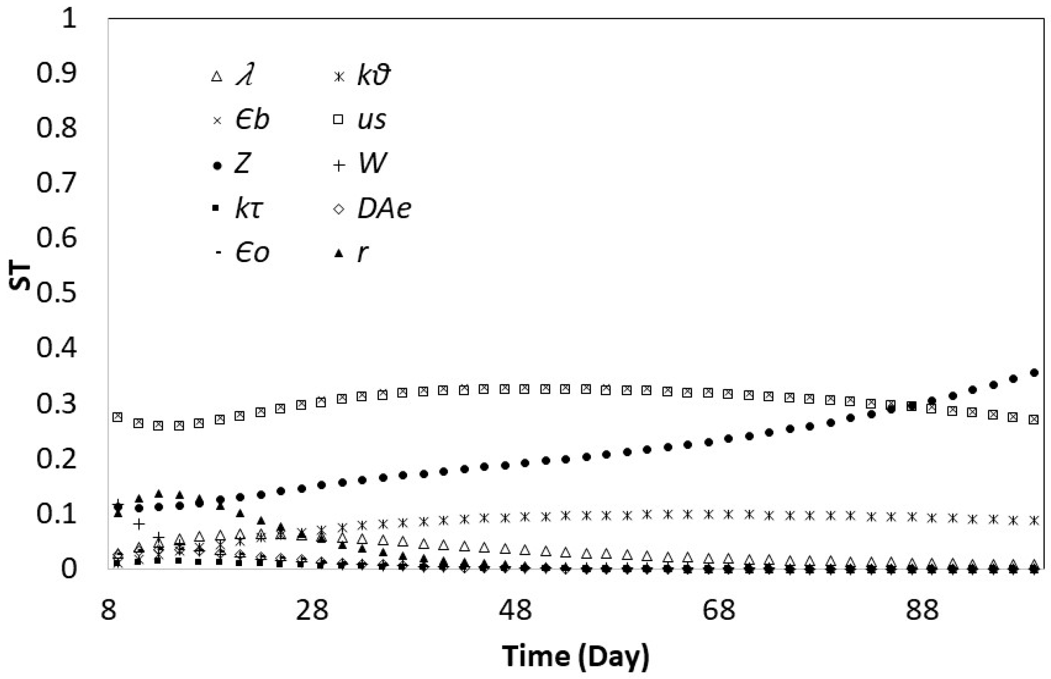
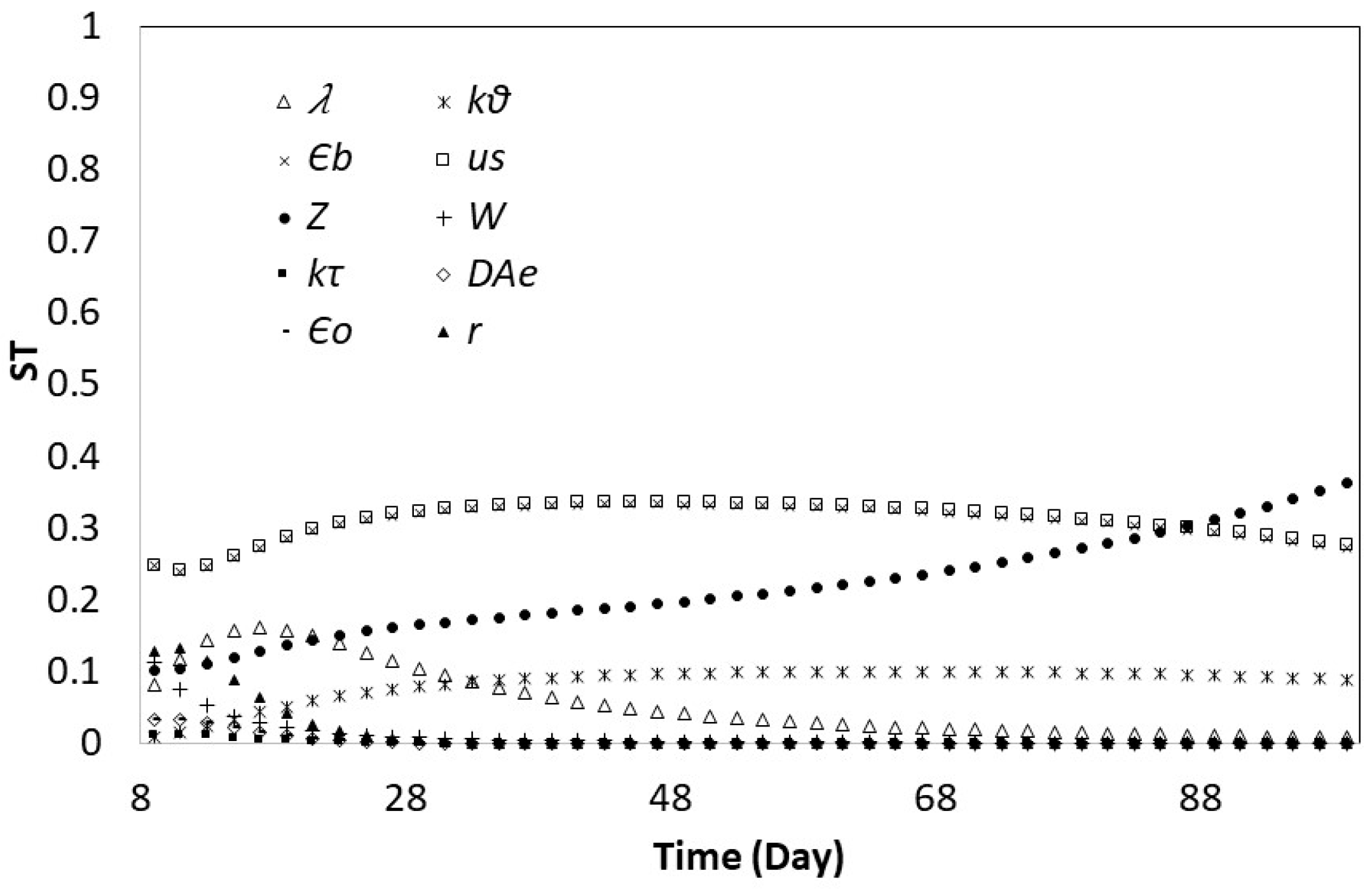
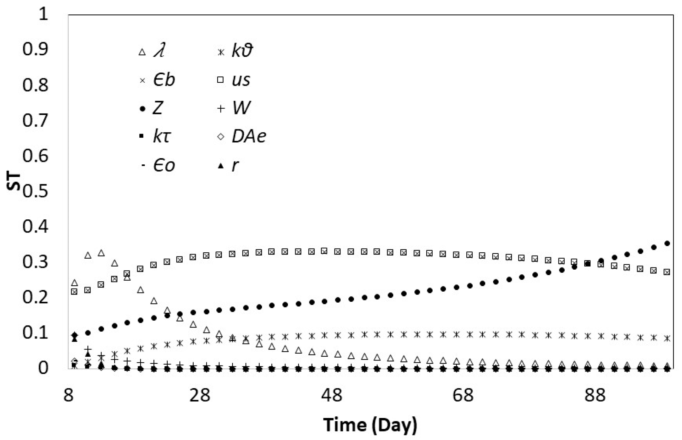
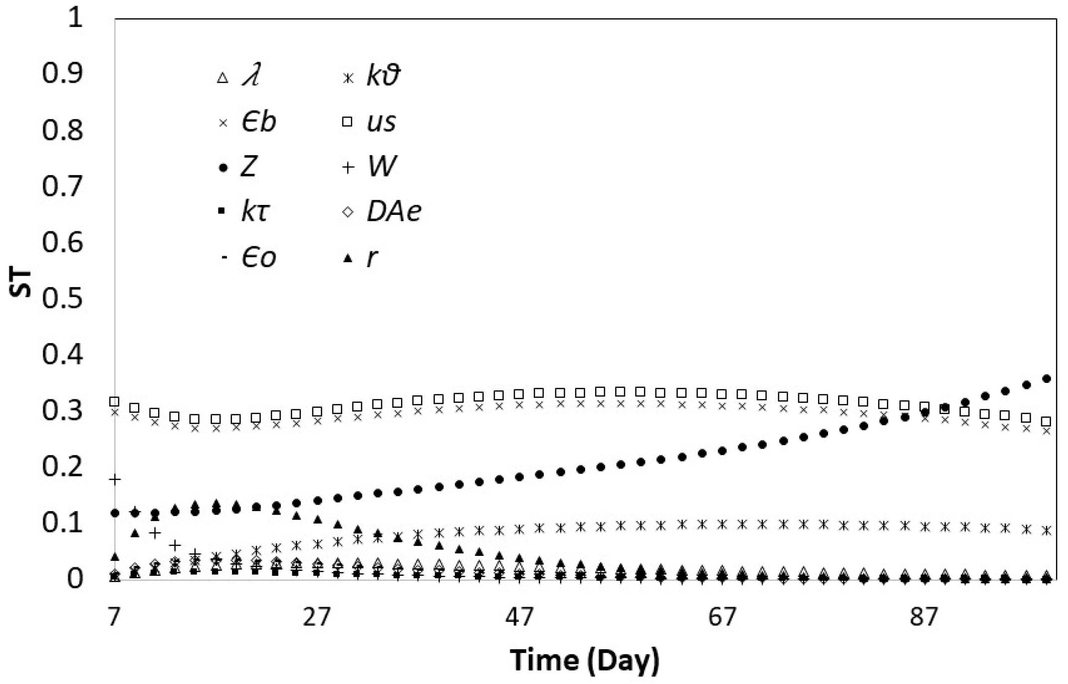
The realization of GSA considered six cases. The first case applies GSA to the kinetic model using the nominal values and the uncertainties used in UA, with leaching time between one and 100 days. In cases two to six, the GSA was realized by modifying the nominal value of one input variable and maintaining the others in their nominal values. The same uncertainties were used in all cases. The second case considered a height of the heap of 300 cm and 900 cm. The third case considered a particle radius of 1.5 cm and 3.5 cm. The fourth case considered a superficial velocity of 9.0 cm3/cm2·d and 57.0 cm3/cm2·d. The fifth case considered an effective diffusivity 0.06 cm3/cm2·d and 0.112 cm3/cm2·d. The sixth case considered a porosity of the particle of 0.01 and 0.06.
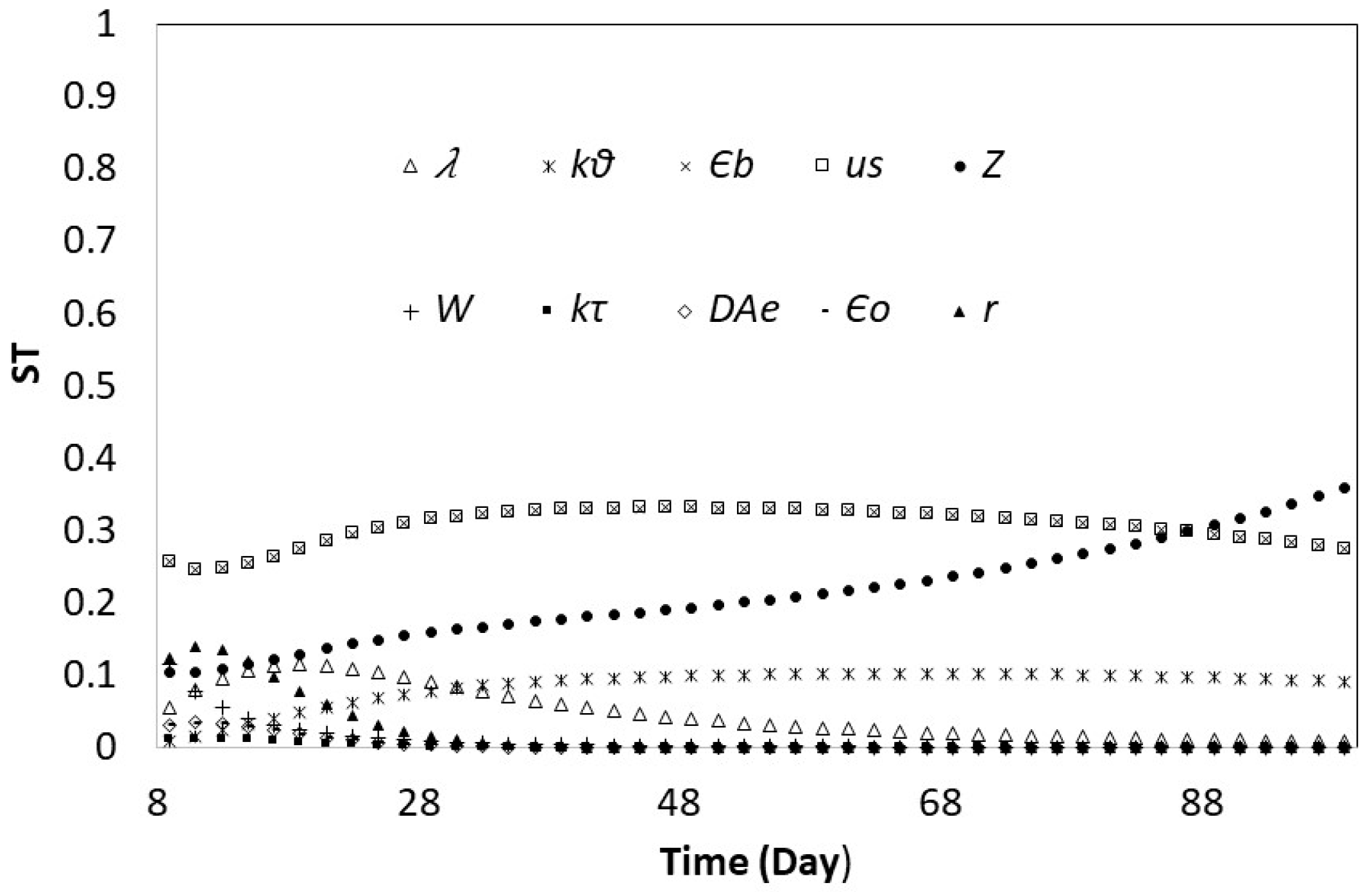
Figure 3 shows the results of the first case. It can be observed that u s and ε b are influential on recovery throughout the leaching time while the influence of Z on recovery increases over time. The influence of λ on recovery increases until approximately day 18 and then decreases over time. The variable k_θ presents a moderate influence on recovery, while input variables r and ω present a low influence on recovery. The remaining input variables do not influence the recovery. These GSA results allow a reduction of the number of input variables of the kinetic model. For example, if non-significant variables are set at their nominal values, Equation (11) can be rewritten as:
R = 132.743 Z 0.0864 + 0.041 ( 1 λ e k θ · u s ε b Z ( t ε b Z ω u s   ) ( 1 λ ) e 0.864 r 2 ( t ε b Z ω u s   ) )
Evidently, these results depend on the uncertainty range of the input variables of the kinetic model. It is important to indicate that these results contradict the results when local SA is applied, which concludes that the model of Equation (11) does not have extra variables [36].
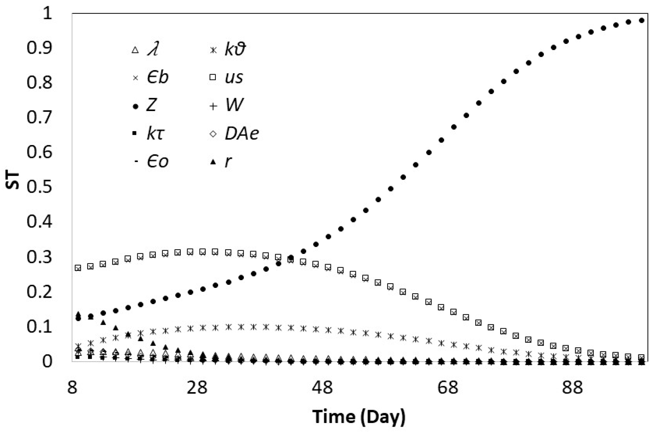
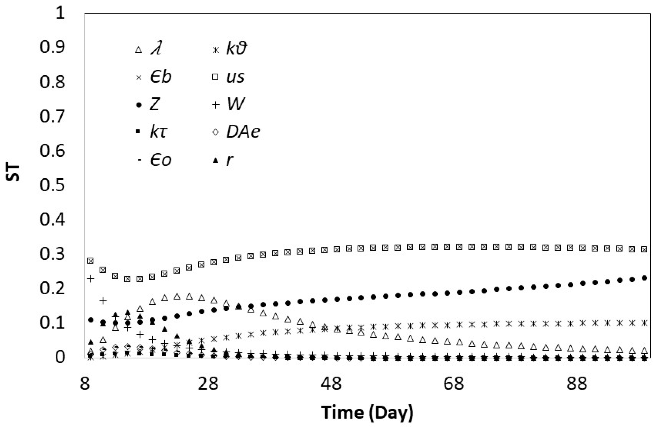
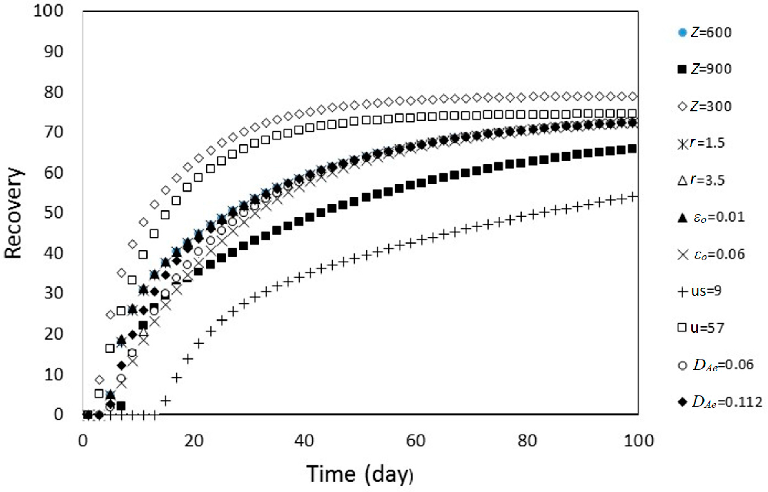
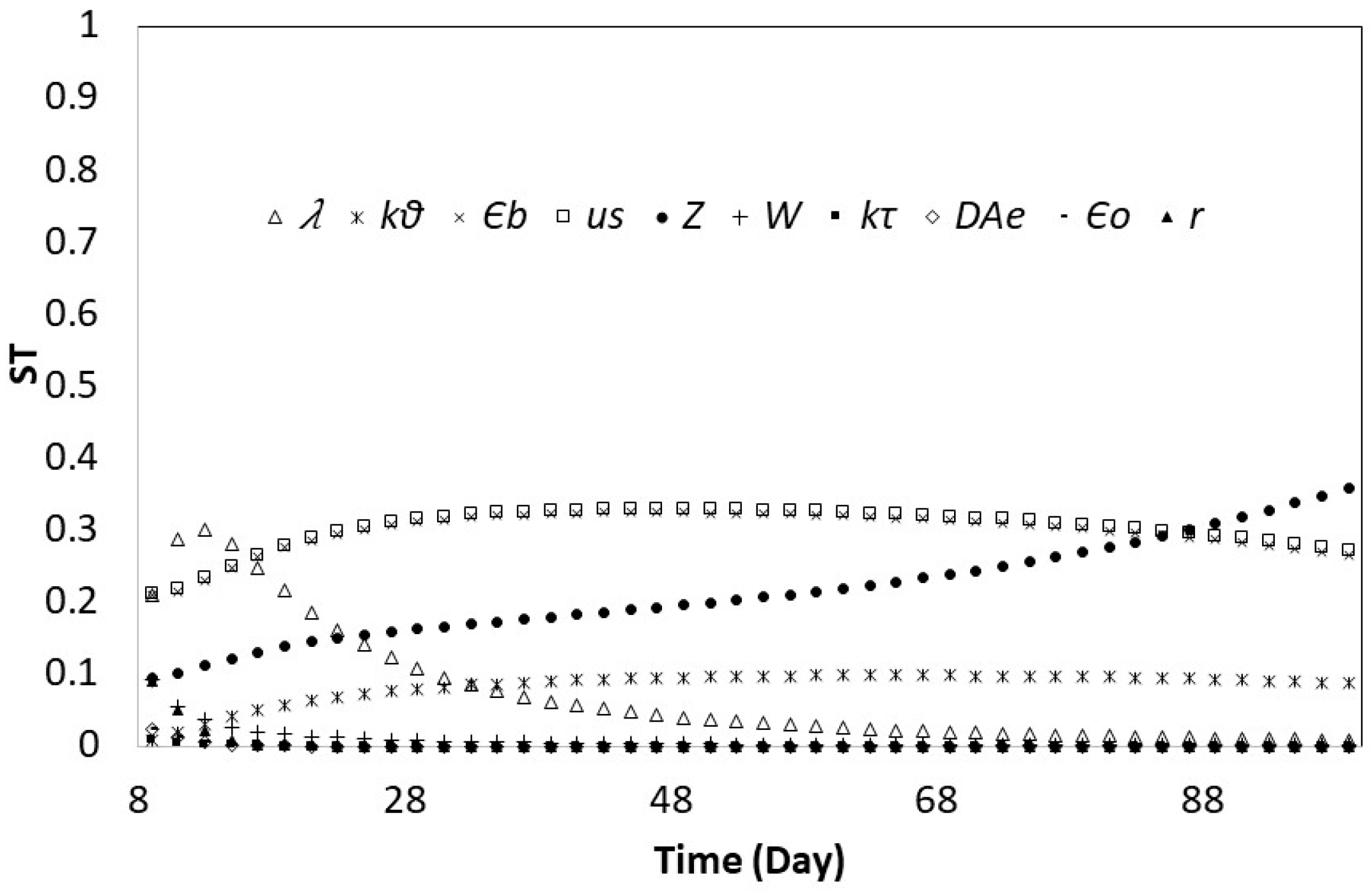
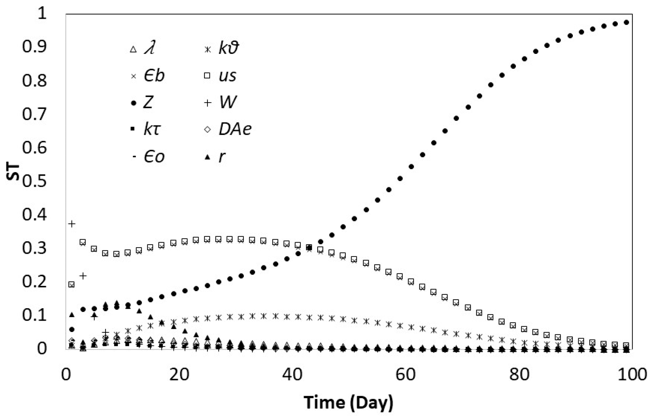
Figure 4 and Figure 5 show the results for the second case; this is for a heap height of 300 and 900 cm. These figures show that when the heap height increases, the S T i of the heap height decreases. These results agree with the kinetic behavior of heap leaching shown in Figure 6. This figure shows that when the height of heap decreases, the recovery is more sensitive to changes in the heap height.
Figure 3, Figure 4 and Figure 5 also show that the relative weight of the significant variables changes if the nominal values of the height of the heap change. To complement the GSA results, Figure 6 shows the recovery versus time for all the cases studied.
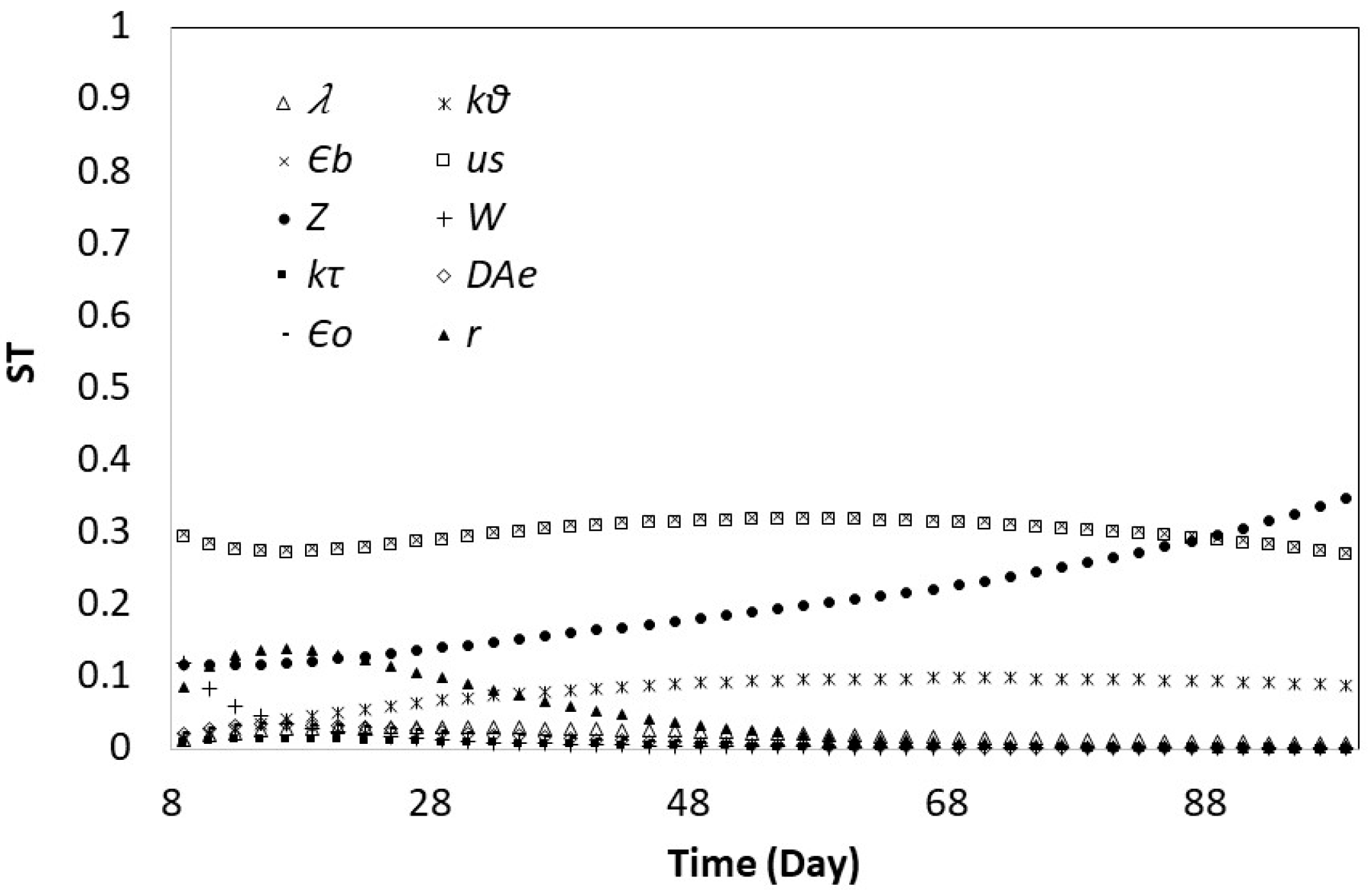
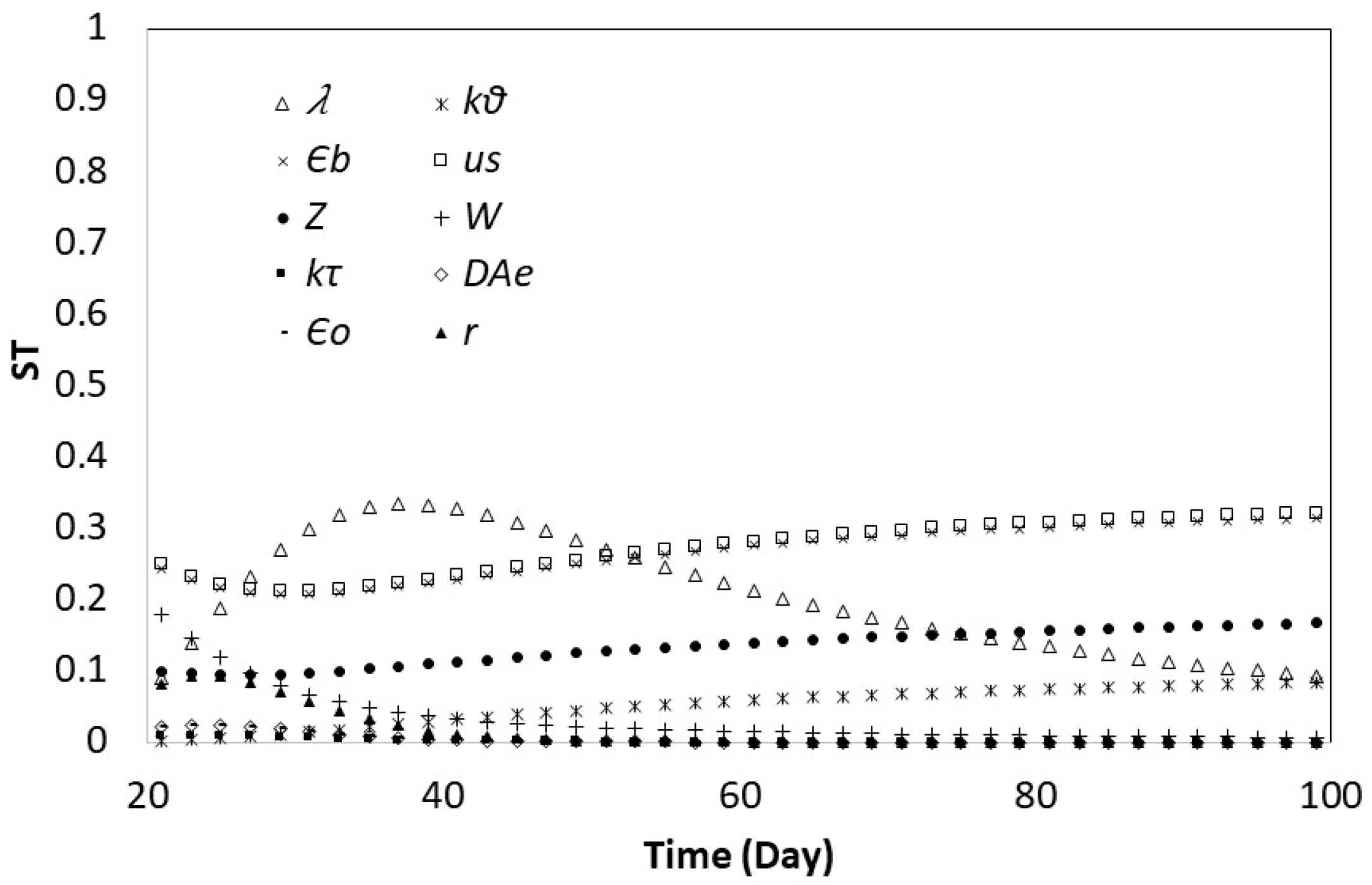
Figure 3, Figure 7 and Figure 8 show the S T i index when the particle radius is 2.5, 1.5 and 3.5 cm. The effect of r is small and only at times less than 50 days, which is consistent with what was observed in the recovery (see Figure 6). The effect of r increases as its value increases and it produces a change in the S T i index of the other input variables. This occurs because the uncertainties were considered as a percentage of the nominal value. Then, at a higher nominal value of a variable, greater uncertainty was considered. This shows that the level of uncertainty plays an important role and that its value must be carefully determined.
Figure 9, Figure 10, Figure 11, Figure 12, Figure 13 and Figure 14 show the results of the other cases. Figure 3, Figure 9 and Figure 10 show the S T i index when the u s is 9.0, 28.0 and 57.0 cm3/cm2·s. Figure 3, Figure 11 and Figure 12 show the S T i index when the D A e is 0.0864, 0.06 and 0.112 cm3/cm2·d. Figure 3, Figure 13 and Figure 14 show the S T i index when the ε o is 0.03, 0.01 and 0.06. The effect of the nominal value and the uncertainty is important in the results observed.
In all cases analyzed, it is observed that the number of input variables of the kinetic model can be reduced. These reductions depend on the uncertainties range of the input variables. This result is different to the one obtained when local SA is applied [36]. Therefore, it is recommended that GSA must be used and not local SA.

3.3. Regionalization

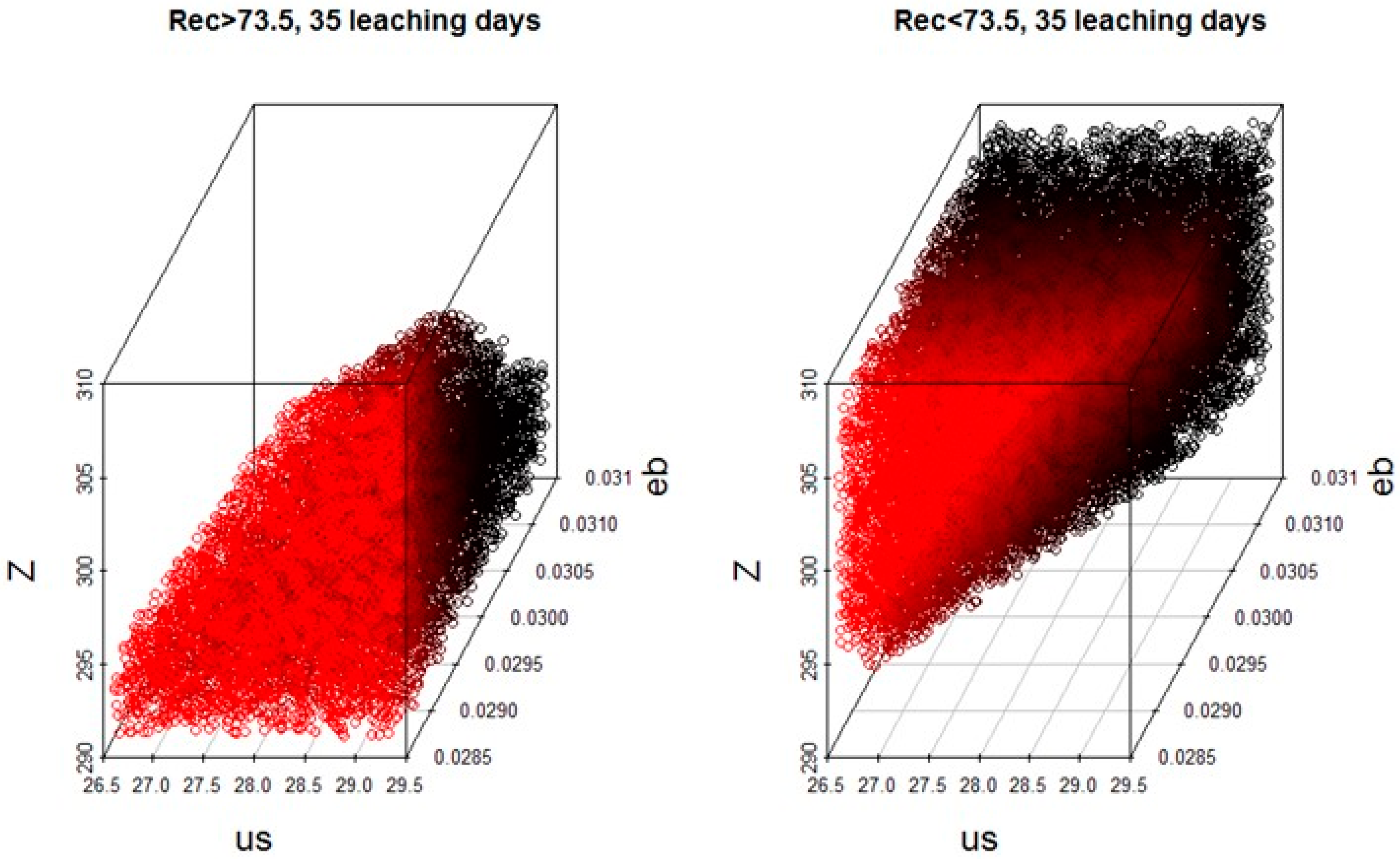
The information obtained with GSA can be used to study some applications of the model. For example, to know the operating conditions necessary to obtain a recovery higher than 73.5% (obtained when the leaching time is approximately equal to 35 days, and heap height is 300 cm). The regionalization of the input variables can give some orientations. The results of GSA at day 35 indicate that the regionalization must be done only for the height of heap, superficial velocity and volumetric fraction of the bulk solution in the bed; the other input variables can be fixed in their current operational values (nominal values). This reduction of the heap leaching model helps to obtain operating regions more defined and easier to interpret. The groups B (desired outcome) and B ¯ (undesired outcome) are defined as follows.
B = { x E / R ( x ) > 73.5 % }
B ¯ = { x E / R ( x ) 73.5 % }
where E is the space formed by the uncertainties of three influential input variables, while R ( x ) is the recovery of heap leaching in the point x. The regions B and B ¯ are shown in Figure 15.
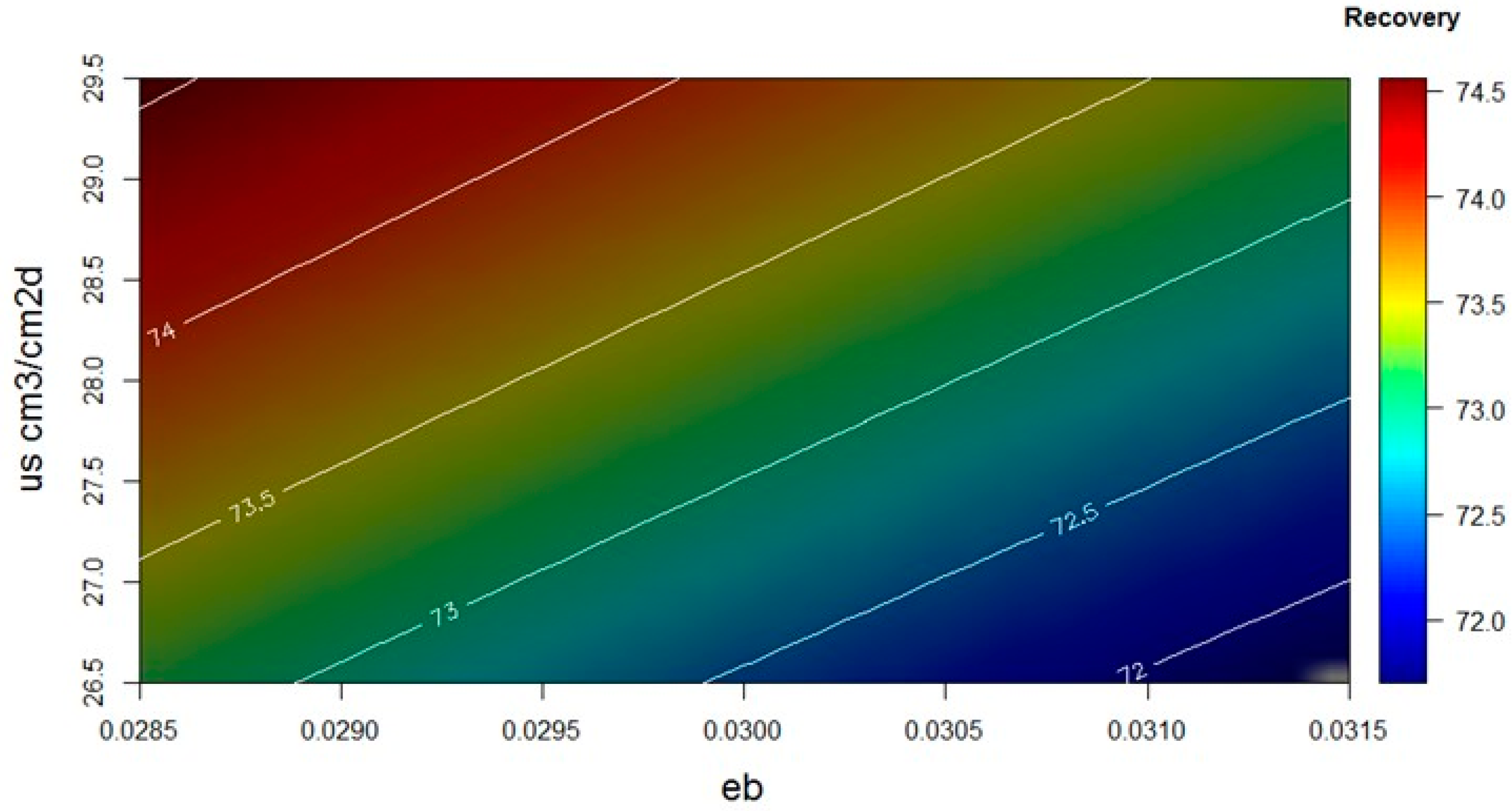
For example, Figure 15 (left) shows the values of the height of heap, superficial velocity, and volumetric fraction of the bulk solution in the bed when the desired outcome is obtained (recovery higher than 73.5%). In fact, if the heap leaching operating conditions are Z = 300 cm, u s = 27   cm 3 / cm 2 · s and ϵ b = 3.0 % (region B ¯ ), the recovery calculated with the Mellado et al. model is 72.7%, but if Z = 300 cm, u s = 29   cm 3 / cm 2 · s and ϵ b = 2.9 % (region B ), the recovery calculated with the Mellado et al. model is 74.1%. The regionalization analysis can be complemented with planes like the ones shown in Figure 16.
Figure 16 shows the plane Z = 300   cm including both regions ( B B ¯ ) . This figure allows us to clearly operate the heap leaching when the leaching time is equal to 35 days. For example, when u s = 28   cm 3 / cm · d , ϵ b begins to increase. Figure 16 shows that the recovery of heap leaching decreases. Therefore, the regionalization of influential input variables allows us to control the uncertainty of recovery of heap leaching. This application indicates that the kinetic model presents versatility.

4. Conclusions

This work shows that UA and GSA are useful tools to test the model robustness against uncertainties in leaching models. The kinetic model proposed by Mellado et al. [27,28] was used as an example. The UA indicates that the kinetic model can estimate the recovery behavior considering the full range of uncertainties of input variables. Different types of PDF for recovery were observed after 35 and 100 days of operation. In addition, the uncertainty in the recovery at day 100 was much less than the uncertainty at day 35. The GSA indicates that the kinetic model is over-parameterized on the uncertainties range considered; this conclusion contradicts the results when local SA is used. The level of uncertainty affects the results, which is why the range of uncertainty must be determined with some degree of certainty. Additionally, the kinetic model presents versatility because it allows determining operating regions for controlling the uncertainty in the recovery of the leaching process. The regionalization of the most significant variables (higher values of S T i ) can be a tool to determine operating conditions or understand the relationship between variables that produce undesired or desired effects.

Acknowledgments

The authors thank CONICYT for funding through Fondecyt 1171341.

Author Contributions

M.E.M., F.A.L. and F.D.S. implemented and performed the UA, GSA and regionalization; L.A.C. and E.D.G. analyzed the results and wrote the paper.

Conflicts of Interest

The authors declare no conflict of interest.

References

  1. Watling, H.R.; Elliot, A.D.; Maley, M.; van Bronswijk, W.; Hunter, C. Leaching of a low-grade, copper–nickel sulfide ore. 1. Key parameters impacting on Cu recovery during column bioleaching. Hydrometallurgy 2009, 97, 204–212. [Google Scholar] [CrossRef]
  2. Parbhakar-Fox, A. Geoenvironmental Characterisation of Heap Leach Materials at Abandoned Mines: Croydon Au-Mines, QLD, Australia. Minerals 2016, 6, 52. [Google Scholar] [CrossRef]
  3. Valencia, J.A.; Méndez, D.A.; Cueto, J.Y.; Cisternas, L.A. Saltpeter extraction and modelling of caliche mineral heap leaching. Hydrometallurgy 2008, 90, 103–114. [Google Scholar]
  4. Moreno, L.; Ordóñez, J.I.; Cisternas, L.A. Dissolution Model of Multiple Species: Leaching of Highly Soluble Minerals. Metall. Mater. Trans. B 2017, 48, 1817–1826. [Google Scholar] [CrossRef]
  5. Negron, L.; Pingitore, N.; Gorski, D. Porosity and Permeability of Round Top Mountain Rhyolite (Texas, USA) Favor Coarse Crush Size for Rare Earth Element Heap Leach. Minerals 2016, 6, 16. [Google Scholar] [CrossRef]
  6. McBride, D.; Gebhardt, J.E.; Croft, T.N.; Cross, M. Modeling the hydrodynamics of heap leaching in sub-zero temperatures. Miner. Eng. 2016, 90, 77–88. [Google Scholar] [CrossRef]
  7. Petersen, J. Heap leaching as a key technology for recovery of values from low-grade ores—A brief overview. Hydrometallurgy 2016, 165, 206–212. [Google Scholar] [CrossRef]
  8. Watling, H. Review of Biohydrometallurgical Metals Extraction from Polymetallic Mineral Resources. Minerals 2014, 5, 1–60. [Google Scholar] [CrossRef]
  9. Marsden, J.O.; Botz, M.M. Heap leach modeling—A review of approaches to metal production forecasting. Miner. Metall. Process. 2017, 34, 53–64. [Google Scholar] [CrossRef]
  10. Ghorbani, Y.; Franzidis, J.-P.; Petersen, J. Heap leaching technology—Current state, innovations and future directions: A review. Miner. Process. Extr. Metall. Rev. 2015, 37, 73–119. [Google Scholar] [CrossRef] [Green Version]
  11. Thiel, R.; Smith, M.E. State of the practice review of heap leach pad design issues. Geotext. Geomembr. 2004, 22, 555–568. [Google Scholar] [CrossRef]
  12. De Andrade Lima, L.R.P. A mathematical model for isothermal heap and column leaching. Braz. J. Chem. Eng. 2004, 21, 435–447. [Google Scholar] [CrossRef]
  13. Bouffard, S.C.; Dixon, D.G. Investigative study into the hydrodynamics of heap leaching processes. Metall. Mater. Trans. B 2001, 32, 763–776. [Google Scholar] [CrossRef]
  14. Bouffard, S.C.; Dixon, D.G. Evaluation of kinetic and diffusion phenomena in cyanide leaching of crushed and run-of-mine gold ores. Hydrometallurgy 2007, 86, 63–71. [Google Scholar] [CrossRef]
  15. Cross, M.; Bennett, C.R.; Croft, T.N.; McBride, D.; Gebhardt, J.E. Computational modeling of reactive multi-phase flows in porous media: Applications to metals extraction and environmental recovery processes. Miner. Eng. 2006, 19, 1098–1108. [Google Scholar] [CrossRef]
  16. Sheikhzadeh, G.A.; Mehrabian, M.A.; Mansouri, S.H.; Sarrafi, A. Computational modelling of unsaturated flow of liquid in heap leaching—Using the results of column tests to calibrate the model. Int. J. Heat Mass Transf. 2005, 48, 279–292. [Google Scholar] [CrossRef]
  17. Gálvez, E.D.; Moreno, L.; Mellado, M.E.; Ordóñez, J.I.; Cisternas, L.A. Heap leaching of caliche minerals: Phenomenological and analytical models—Some comparisons. Miner. Eng. 2012, 33, 46–53. [Google Scholar] [CrossRef]
  18. Mellado, M.E.; Cisternas, L.A. An analytical-numerical method for solving a heap leaching problem of one or more solid reactants from porous pellets. Comput. Aided Chem. Eng. 2008, 25, 877–882. [Google Scholar]
  19. Bouffard, S.C.; Dixon, D.G. Heap biooxidation of refractory gold ores: Current state of the art. Miner. Process. Extr. Metall. Rev. 2004, 25, 159–192. [Google Scholar] [CrossRef]
  20. Bennett, C.R.; McBride, D.; Cross, M.; Gebhardt, J.E. A comprehensive model for copper sulphide heap leaching. Hydrometallurgy 2012, 127–128, 150–161. [Google Scholar] [CrossRef]
  21. McBride, D.; Croft, T.N.; Cross, M.; Bennett, C.; Gebhardt, J.E. Optimization of a CFD—Heap leach model and sensitivity analysis of process operation. Miner. Eng. 2014, 63, 57–64. [Google Scholar] [CrossRef]
  22. Hoseinian, F.S.; Abdollahzade, A.; Mohamadi, S.S.; Hashemzadeh, M. Recovery prediction of copper oxide ore column leaching by hybrid neural genetic algorithm. Trans. Nonferrous Met. Soc. China 2017, 27, 686–693. [Google Scholar] [CrossRef]
  23. Lane, W.A.; Ryan, E.M. Verification, validation, and uncertainty quantification of a sub-grid model for heat transfer in gas-particle flows with immersed horizontal cylinders. Chem. Eng. Sci. 2018, 176, 409–420. [Google Scholar] [CrossRef]
  24. Ordóñez, J.I.; Moreno, L.; Mellado, M.E.; Cisternas, L.A. Modeling validation of caliche ore leaching using seawater. Int. J. Miner. Process. 2014, 126, 10–17. [Google Scholar] [CrossRef]
  25. Ordóñez, J.; Condori, A.; Moreno, L.; Cisternas, L. Heap Leaching of Caliche Ore. Modeling of a Multicomponent System with Particle Size Distribution. Minerals 2017, 7, 180. [Google Scholar] [CrossRef]
  26. Liddell, K.C. Shrinking core models in hydrometallurgy: What students are not being told about the pseudo-steady approximation. Hydrometallurgy 2005, 79, 62–68. [Google Scholar] [CrossRef]
  27. Mellado, M.E.; Cisternas, L.A.; Gálvez, E.D. An analytical model approach to heap leaching. Hydrometallurgy 2009, 95, 33–38. [Google Scholar] [CrossRef]
  28. Mellado, M.E.; Casanova, M.P.; Cisternas, L.A.; Gálvez, E.D. On scalable analytical models for heap leaching. Comput. Chem. Eng. 2011, 35, 220–225. [Google Scholar] [CrossRef]
  29. Ding, D.; Song, J.; Ye, Y.; Li, G.; Fu, H.; Hu, N.; Wang, Y. A kinetic model for heap leaching of uranium ore considering variation of model parameters with depth of heap. J. Radioanal. Nucl. Chem. 2013, 298, 1477–1482. [Google Scholar] [CrossRef]
  30. Dixon, D.G.; Hendrix, J.L. A general model for leaching of one or more solid reactants from porous ore particles. Metall. Trans. B 1993, 24, 157–169. [Google Scholar] [CrossRef]
  31. Dixon, D.G.; Hendrix, J.L. A mathematical model for heap leaching of one or more solid reactants from porous ore pellets. Metall. Trans. B 1993, 24, 1087–1102. [Google Scholar] [CrossRef]
  32. Saltelli, A.; Annoni, P. How to avoid a perfunctory sensitivity analysis. Environ. Model. Softw. 2010, 25, 1508–1517. [Google Scholar] [CrossRef]
  33. Saltelli, A.; Tarantola, S.; Campolongo, F. Sensitivity analysis as an ingredient of modeling. Stat. Sci. 2000, 15, 377–395. [Google Scholar]
  34. Lilburne, L.; Tarantola, S. Sensitivity analysis of spatial models. Int. J. Geogr. Inf. Sci. 2009, 23, 151–168. [Google Scholar] [CrossRef]
  35. Gálvez, E.D.; Capuz-Rizo, S.F. Assessment of global sensitivity analysis methods for project scheduling. Comput. Ind. Eng. 2016, 93, 110–120. [Google Scholar] [CrossRef]
  36. Mellado, M.E.; Gálvez, E.D.; Cisternas, L.A. A posteriori analysis of analytical models for heap leaching. Miner. Metall. Process. 2012, 29, 103. [Google Scholar]
  37. Mellado, M.E.; Gálvez, E.D.; Cisternas, L.A. On the optimization of flow rates on copper heap leaching operations. Int. J. Miner. Process. 2011, 101, 75–80. [Google Scholar] [CrossRef]
  38. Ordóñez, J.I.; Moreno, L.; Gálvez, E.D.; Cisternas, L.A. Seawater leaching of caliche mineral in column experiments. Hydrometallurgy 2013, 139, 79–87. [Google Scholar] [CrossRef]
  39. Saltelli, A. Sensitivity Analysis for Importance Assessment. Risk Anal. 2002, 22, 579–590. [Google Scholar] [CrossRef] [PubMed]
  40. Reuter, U.; Liebscher, M. Global Sensitivity Analysis in View of Nonlinear Structural Behavior; LS-DYNA Anwenderforum: Bamberg, Germany, 2008; Volume 56. [Google Scholar]
  41. Iooss, B.; Lemaître, P. A Review on Global Sensitivity Analysis Methods. Uncertain. Manag. Simul.-Optim. Complex Syst. 2015, 59, 101–122. [Google Scholar]
  42. Saltelli, A.; Annoni, P.; Azzini, I.; Campolongo, F.; Ratto, M.; Tarantola, S. Variance based sensitivity analysis of model output. Design and estimator for the total sensitivity index. Comput. Phys. Commun. 2010, 181, 259–270. [Google Scholar] [CrossRef]
  43. Sobol, I.M. Sensitivity analysis for non-linear mathematical models. Math. Comput. Simul. 1993, 1, 407–414. [Google Scholar]
  44. Spear, R.; Hornberger, G.M. Eutrophication in peel inlet—II. Identification of critical uncertainties via generalized sensitivity analysis. Water Res. 1980, 14, 43–49. [Google Scholar] [CrossRef]
  45. Lucay, F.; Cisternas, L.A.; Gálvez, E.D. Global sensitivity analysis for identifying critical process design decisions. Chem. Eng. Res. Des. 2015, 103, 74–83. [Google Scholar] [CrossRef]
  46. Jansen, M.J.W. Analysis of variance designs for model output. Comput. Phys. Commun. 1999, 117, 35–43. [Google Scholar] [CrossRef]
  47. Pujol, G.; Iooss, B.; Janon, A. Global Sensitivity Analysis of Model Output, version 1.15.0; R Package; 2017. Available online: https://CRAN.R-project.org/package=sensitivity (accessed on 26 January 2018).
  48. R: A Language and Environment for Statistical Computing; R Core Team (2013); R Foundation for Statistical Computing: Vienna, Austria, 2013; Available online: http://www. R-project.org (accessed on 26 January 2018).
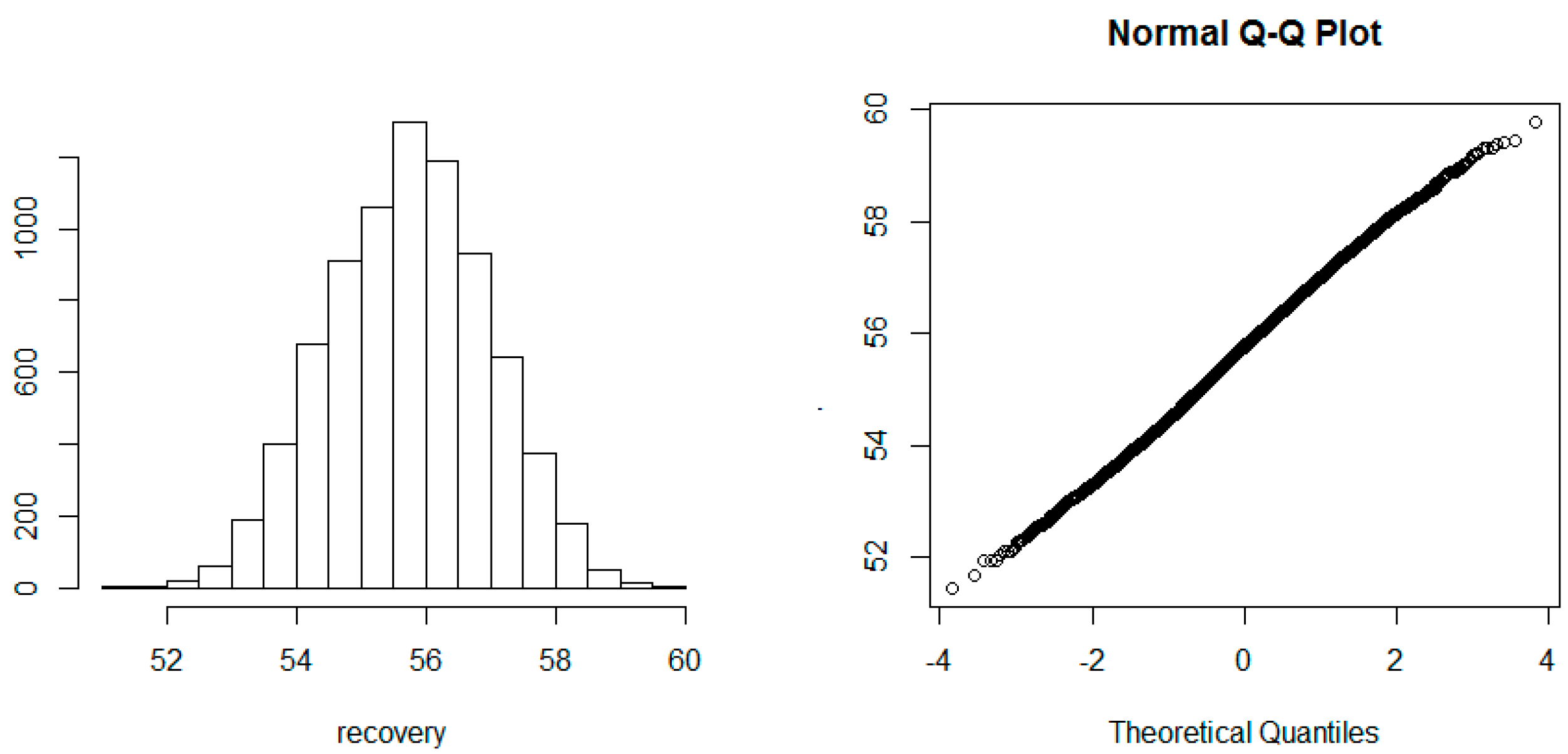
Figure 1. Uncertainty analysis at 30 days of leaching.
Minerals 08 00044 g001
Figure 2. Uncertainty analysis at 100 days of leaching.
Minerals 08 00044 g002
Figure 3. Global sensitivity analysis (GSA) of the model with a heap height equal to 600 cm.
Minerals 08 00044 g003
Figure 4. GSA of the model with a heap height equal to 300 cm.
Minerals 08 00044 g004
Figure 5. GSA of the model at a heap height of 900 cm.
Minerals 08 00044 g005
Figure 6. Recovery behavior of heap leaching, cases 1–6.
Minerals 08 00044 g006
Figure 7. GSA of the model at radius 1.5 cm.
Minerals 08 00044 g007
Figure 8. GSA of the model at radius 3.5 cm.
Minerals 08 00044 g008
Figure 9. GSA of the model at u s 9.0 cm3/cm2·s.
Minerals 08 00044 g009
Figure 10. GSA of the model at u s 57.0 cm3/cm2·s.
Minerals 08 00044 g010
Figure 11. GSA of the model at D A e 0.06 cm3/cm2·d.
Minerals 08 00044 g011
Figure 12. GSA of the model at D A e 0.112 cm3/cm2·d.
Minerals 08 00044 g012
Figure 13. GSA of the model at ε o 0.01.
Minerals 08 00044 g013
Figure 14. GSA of the model at ε o 0.06.
Minerals 08 00044 g014
Figure 15. Regionalization of the influential input variables Z , u s and ϵ b , B (left) and B ¯ (right).
Minerals 08 00044 g015
Figure 16. Plane Z = 300   cm including both groups B (desired outcome, recovery >73.5%) and B ¯ (undesired outcome, recovery <73.5%)
Minerals 08 00044 g016