Linkages between the Genesis and Resource Potential of Ferromanganese Deposits in the Atlantic, Pacific, and Arctic Oceans

Menendez, Amaya; James, Rachael; Shulga, Natalia; Connelly, Doug; Roberts, Steve

doi:10.3390/min8050197

Open AccessEditor’s ChoiceArticle

Linkages between the Genesis and Resource Potential of Ferromanganese Deposits in the Atlantic, Pacific, and Arctic Oceans

¹

Ocean and Earth Science, National Oceanography Centre Southampton, University of Southampton Waterfront Campus, European Way, Southampton SO14 3ZH, UK

²

Shirshov Institute of Oceanology, Russian Academy of Sciences, 36, Nakhimovsky prt., 117997 Moscow, Russia

³

National Oceanography Centre, University of Southampton Waterfront Campus, European Way, Southampton SO14 3ZH, UK

^*

Author to whom correspondence should be addressed.

Minerals 2018, 8(5), 197; https://doi.org/10.3390/min8050197

Submission received: 6 March 2018 / Revised: 26 April 2018 / Accepted: 3 May 2018 / Published: 5 May 2018

(This article belongs to the Special Issue Deep-Sea Minerals and Gas Hydrates)

Download

Browse Figures

Versions Notes

Abstract

:

In addition to iron and manganese, deep sea ferromanganese deposits, including nodules and crusts, contain significant amounts of economically interesting metals, such as cobalt (Co), nickel (Ni), copper (Cu), and rare Earth elements and yttrium (REY). Some of these metals are essential in the development of emerging and new-generation green technologies. However, the resource potential of these deposits is variable, and likely related to environmental conditions that prevail as they form. To better assess the environmental controls on the resource potential of ferromanganese deposits, we have undertaken a detailed study of the chemical composition of ferromanganese nodules and one crust sample from different oceanic regions. Textural and chemical characteristics of nodules from the North Atlantic and a crust from the South Pacific suggest that they acquire metals from a hydrogenous source. These deposits are potentially an economically important source of Co and the REY. On the other hand, nodules from the Pacific Ocean represent a marginal resource of these metals, due to their relatively fast growth rate caused by diagenetic precipitation. By contrast, they have relatively high concentrations of Ni and Cu. A nodule from the Arctic Ocean is characterised by the presence of significant quantities of detrital silicate material, which significantly reduces their metal resource.

Keywords:

polymetallic nodules; deep sea mining; ferromanganese crusts; diagenesis; Arctic nodules

Graphical Abstract

1. Introduction

Marine ferromanganese deposits, including polymetallic nodules and crusts, are important resources of metals such as Co, Ni, Cu, Mo, Li, and Te, as well as the rare Earth elements and yttrium (REY) [1]. Crusts also contain relatively high concentrations of platinum [2,3], as well as smaller amounts of Rh, Ru, Os, Pd, and Ir. Ferromanganese deposits are distributed throughout the world’s ocean basins, but their chemical and mineralogical compositions and, hence, their resource potential, can be variable (e.g., [2,3,4,5,6,7]).

Polymetallic ferromanganese nodules generally occur in the deepest parts of the ocean basins at depths ranging between 3500 to 6500 m [8], although they can also be found at much shallower depths [5].

Ferromanganese crusts usually form on the top and slopes of seamounts, ridges, and plateaus. Both types of deposits have a complex internal structure, and some can form extremely slowly (~1 to up to 250 mm/Ma) [9] by deposition of Fe- and Mn-rich microlayers around a nucleus. These microlayers have distinct chemical and mineralogical compositions which reflect the environmental conditions in both the ocean and the host sediments at the time of deposition. Three different types of ferromanganese deposit have been recognised: (1) hydrogenous, whereby the deposit acquires metals from the overlying oxic water column [10]; (2) diagenetic, whereby metals are acquired from either oxic or sub-oxic sediment pore waters [11]; and (3) hydrothermal, where hydrothermal vent fluids are the principal source of metals [10]. The chemical and mineralogical composition of ferromanganese crusts can also be modified after deposition by diagenetic processes, including phosphatization (e.g., [12]).

Hydrogenous deposits typically have rather low Mn/Fe ratios, ≤3, and low quantities of Ni and Cu, whereas diagenetic deposits have higher Mn/Fe (3 to >10) and high Ni and Cu [13]. Hydrothermal deposits, in turn show the lowest average Mn/Fe ratios of <1, as well as the lowest content of trace metals [14].

The REY composition of the deposits can also be a useful tracer of the environment of deposition. Hydrogenetic nodules and non-phosphatized crusts tend to have positive Ce anomalies, negative Y anomalies and high Nd concentrations (>100 ppm), whereas diagenetic precipitates usually have negative Ce anomalies, negative Y anomalies, and intermediate Nd concentrations of between 10 and 100 ppm [12]. The REY content of hydrothermal deposits is highly variable (e.g., [14], but, in general, these deposits have negative Ce anomalies, positive Eu and Y anomalies, and are strongly depleted in the light rare Earth elements (LREE) relative to the heavy rare Earth elements (HREE) (e.g., [10,14]). Phosphatized crusts can be identified by positive Ce and positive Y anomalies, and depletion in the LREE relative to the HREE [12].

Changes in environmental conditions mean that the mode of formation may change over time. The oldest (27.8–24.5 Ma) layers in ferromanganese crusts from seamounts in the northeastern tropical Atlantic have relatively high Mn/Fe related to low oxygen conditions, whereas layers deposited during the interval 24.5–16 Ma have lower Mn/Fe, reflecting increased ventilation due to upwelling of oxygenated bottom waters [15]. Similarly, the outermost layers of nodules from the equatorial Eastern Pacific have relatively low Mn/Fe relecting hydrogenetic precipitation from oxygenated waters, whereas some layers in the innermost parts of the nodule have much higher Mn/Fe that are thought to reflect reduced oxygen concentrations due to increased biological productivity in surface waters and/or increased ventilation of bottom waters [16]. Phosphatization of ferromanganese crusts have also been shown to occur under reduced oxygen (sub-oxic) conditions (e.g., [17]).

The mode of formation of ferromanganese deposits usually assessed on the basis of analysis of bulk samples. However, it is clear from studies of nodules from the eastern equatorial Pacific (Clarion-Clipperton Fracture Zone and Peru Basin) that there can be significant differences in the compositions of the individual layers that make up a deposit [18], which reflect changes in the environment of deposition over time. Thus, to better evaluate the environmental controls on the resource potential of deep-ocean ferromanganese deposits, we have undertaken detailed geochemical and textural studies of individual layers within ferromanganese deposits from different environmental settings within the North Atlantic, Central and South Pacific, and Arctic Oceans.

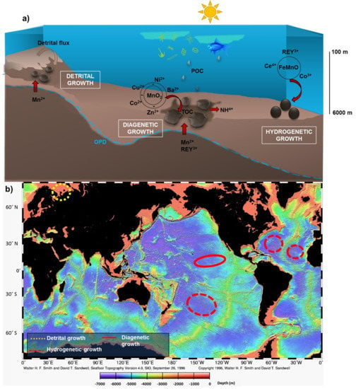
2. Geological Setting

Nodules and crusts for this study were obtained from a number of locations in the Northeast and West Atlantic, the Northeast Kara Sea in the Arctic Ocean, the South and Central Pacific, and the Clarion Clipperton Fracture Zone (CCFZ) in the eastern equatorial Pacific Ocean (Figure 1 and Table 1).

The North Atlantic is characterised by relatively high sedimentation rates due to deposition of authigenic carbonates and a high input of terrigenous material delivered by turbidites (e.g., [19,20]). Ferromanganese nodules are generally confined to deep basins below the carbonate compensation depth (CCD) [21]. The Madeira Basin in East North Atlantic is the deepest part of the Canary Basin, extending from approximately 40° N, 30° E to 20° N, −5° E. Most of its surface is covered by thick turbiditic muds, however, nodule-hosting thin pelagic intervals with lower sedimentation rates also occur in some parts of the basin [22]. The Nares Abyssal Plain in the Western North Atlantic (~ 22° N, −65° E to ~20° N, −62° E) is characterised by the presence of NW–SE trending fractures, which generate turbidite-rich valleys and red clay-rich abyssal hills, where nodules are found [21]. Both the Madeira and the Nares Abyssal Plains are affected by the presence of large gyre systems that keep surface biological productivity low [21,22]. As a result, the total organic carbon content of the sediments is low and the surface sediments are usually oxic. Nodules, therefore, usually form via hydrogenous, rather than diagenetic, processes (e.g., [20,21]).

A similar scenario is found in the Southwest Pacific nodule-forming basin. The sediments in this area are affected by the South Pacific gyre, and subsequently the extremely low respiration rates in the sediments allow oxygen to penetrate the sediment column to the basement [23]. Nodules in this area are found on top of the pelagic brown-red zeolitic clays of the Samoa and Penrhyn basins, extending from approximately −5° N, −170° E to −40° N, −155° E. Nodule formation in these basins is mainly hydrogenetic, being further favoured by the low sedimentation rates, the presence of strong bottom currents and the abundant nuclei particulates [24].

Nodule fields in the Pacific are more extensive than in the other ocean basins, due to lower sedimentation rates and a shallower CCD, which favours the existence of large areas of brown clay-rich sediments where nodules can grow (e.g., [25,26]). The Clarion-Clipperton Fracture Zone (CCFZ) hosts one of the largest nodule fields in the Pacific (e.g., [6]) and it is located in the Central Eastern Pacific Ocean, north of the equatorial high-productivity zone [27]. It extends from approximately 20° N, −120° E to 5° N, −160° E, and is constrained by the Clarion Fracture Zone to the north and the Clipperton Fracture Zone to the south, with a total length of ~7240 km. These fractures are SW–NE trending, as they respond to the north-westward migration of the Pacific Plate [28]. Nodules in the CCFZ are thought to be formed through metal precipitation from both sediment porewaters (diagenetic) and bottom waters (hydrogenetic) [6,18]. Fluctuations in surface bioproductivity caused by plate motion since the Miocene has likely influenced the mode of nodule growth [6]. Present day bioproductivity is lower than it was in the past, and increases from east to west [28].

The crust-forming region of the Cook Austral Chain is part of the larger Southwestern Pacific seamount province [29], located to the west of the Northeast Pacific basin (−30° N, −140° E to 0° N, −150° E). The Western Pacific is characterised by active tectonics and associated volcanism, which has originated a series of NW–SE trending chains of islands and seamounts extending for several thousands of km. Due to the action of the South Pacific Gyre, oxygenated sediment-free conditions prevail throughout the area and, as a consequence, Fe-Mn crusts precipitate from bottom waters (hydrogenetic) onto the surface of seamounts [11]. The greatest abundance of ferromanganese crusts is found on slopes of 0–20° on the top of the seamounts, and crust thicknesses have been found to increase from south to north and from east to west [29].

The Kara Sea is a marginal sea on the continental shelf of Northern Eurasia extending north from the West Siberian Basin from approximately 85° N, 55° E to 70° N, 90° E. It is characterized by a complicated bottom relief with depths not exceeding 150 m. With the exception of a few months in the summer, the Kara Sea is covered by an ice sheet up to 4 m thick for most of the year, which depresses biological productivity in the area [30]. Surface circulation in the southwest part of the sea is controlled by a cyclonic gyre, whereas in the central part it is strongly affected by discharge of northward propagating fresh waters from the Ob and Yenisei Rivers [31]. The distribution of sediment facies is controlled by river discharge of terrigenous material and bottom topography. Sediments on the inner shelf generally consist of silty-sandy clays, while sediments deposited on the outer shelf generally consist of brown to dark brown clays with a small amount of silt and sand [30]. Flat, discoidal-shaped ferromanganese concretions with growth rings are found only on sediments that have a thin oxic surface layer [32].

3. Materials and Methods

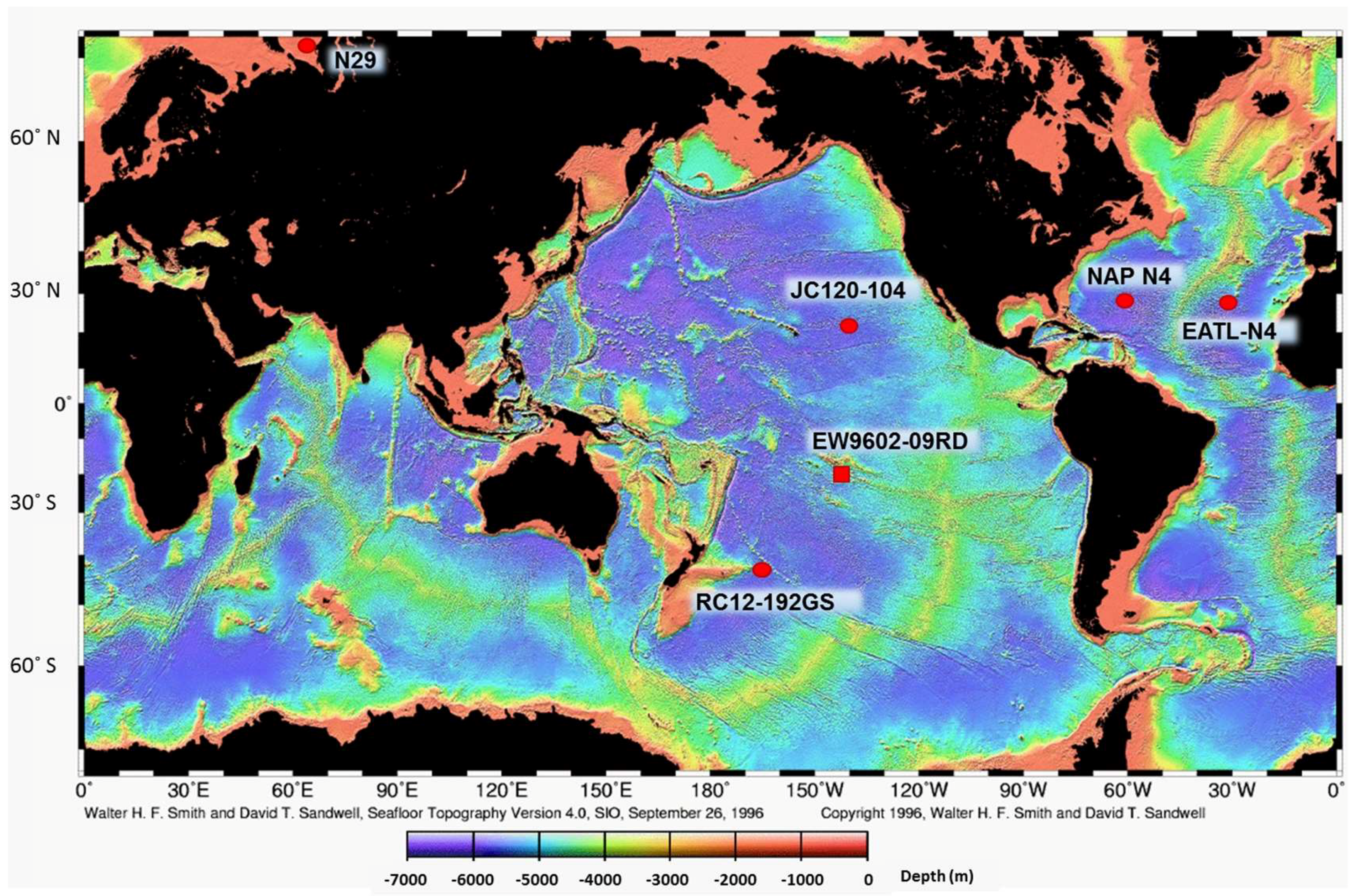
3.1. Samples

Samples E Atl-N4 and NAP-N4 in this study were supplied by the British Ocean Sediment Core Facility (BOSCORF); samples EW9602-09RD and RC12-192GS came from the Lamont-Doherty Earth Observatory, New York (LDEO); sample PSh-125.29(1) was supplied by the Shirshov Institute of Oceanology (Russia) during the RSS Professor Shtockman cruise in October 2013; and sample JC120-104 was collected from CCFZ (UK Claim Area) during the RRS James Cook cruise JC120 in spring 2015.

The nodules range in size from ~1 cm to ~12 cm in diameter. The nodules from the Southwest Pacific Basin and the Atlantic Ocean are generally rounded and have a smooth surface. Similar morphological features have been described in nodules from the vicinity of the Cook Islands [24], and in nodules from the North Atlantic [21], at water depths of >5000 m. By contrast, the larger nodule from the CCFZ has a botryoidal appearance and a complex internal structure. These features are typical of nodules from this area at depths of 3000–4000 m (e.g., [6,8,18]).

The nodule from the Kara Sea in the Arctic Ocean (sample PSh-125.29(1)) is, by contrast, oblate and has a discoid shape with a long axis of ~7 cm. Similar flattened concretions have been reported in other shallow-water regions of the Kara Sea [35], as well as in the Chukchi and East Siberian Seas [36].

The ferromanganese crust sample EW9602-09RD was dredged from a seamount from the western part of the Challenger Fracture Zone. It has a botryoidal, slightly irregular appearance, similar to crusts recovered from other South Pacific seamount chains at depths of between 400 and 4000 m [11].

3.2. Analytical Methods

3.2.1. Scanning Electron Microscopy (SEM)

The crust and the nodules were prepared for SEM analysis by sectioning, and grinding and polishing with epoxy resin until a flat surface was obtained. Sections were then ground down to a thickness of ~100 µm, and mounted onto a glass sample holder.

SEM work was carried out at the University of Southampton using a LEO1450 variable pressure scanning electron microscope (Carl Zeiss, Oxford Instruments, Abingdon, UK). The microstructure of the sectioned crusts and nodules was assessed using both a secondary electron detector (for topographic imaging) and a backscattered electron detector (for compositional analysis). Major element concentrations were determined using energy-dispersive X-ray spectroscopy (EDS; Oxford Instruments, Abingdon, UK, X-Act 10 mm² area SDD with a silicon drift detector) combined with Aztec Energy software (Oxford Instruments, Abingdon, UK). Analyses were conducted at 20 kV, using a probe current of 700 pA and a working distance of 15 mm. The probe current was calibrated on a Faraday cup, and element concentrations were calibrated against various mineral standards from Micro-Analysis Consultants Ltd., Cambridge, UK, and the Natural History Museum, UK. A basalt glass standard reference material (BRR-1) was used to monitor the accuracy of the analyses. Elemental maps were made using a nominal probe current of 2.5–3.0 nA.

3.2.2. Laser Ablation Inductively-Coupled Plasma Mass Spectrometry (LA ICP-MS) Analysis

Laser ablation ICP-MS analyses were used to assess element concentrations in individual layers within the crust and nodules. The analyses were carried out on 100 µm-thick polished sections. Polished chips of NIST 610, NIST 612 and NIST 614 glass standard reference materials were mounted on a glass sample holder. Analyses were conducted at the University of Southampton using a 193 nm excimer laser (New Wave Research model UP193X, New Wave Research, Inc., Fremont, CA, USA) coupled to a quadrupole ICP-MS (Thermo X-Series II). Element concentrations of major elements (Mn and Fe) and trace elements (Ti, V, Co, Ni, Cu, Zn, Ba, Th, and U) and REY (La, Ce, Pr, Nd, Sm, Eu, Gd, Tb, Dy, Y, Ho, Er, Tm, Yb, and Lu) were determined on 50–75 µm diameter spots targeting individual layers in the nodules. Point analyses were performed at intervals of 0.2 to 1 mm. Ablations were conducted with a laser power of ~75% and a repetition rate of 5 Hz, in a He atmosphere. For each analysis, the gas blank was measured first with the laser beam blocked by a shutter. The shutter was then removed, and the transient signals from the analyte were collected for the ablation period. Raw counts were processed offline using standard spreadsheet software, and counts were calibrated using pressed pellets of nodule reference materials NOD-A-1 and NOD-P-1. The accuracy and reproducibility of the measurements was assessed by multiple (n = 60) analyses of NIST 614, NIST 612, and NIST 610 certified reference materials. The external reproducibility of the analyses was better than ±9% for the major elements, better than ±10% for most of the trace elements and better than ±7% for most of the REY, except for Ni (±21%), Cu (±17%), Zn (±13%), Nd (±9%), Sm (±8%), and Gd (±10%). Measured concentrations were within the certified or recommended values for all elements, except Ti (±20%), Mn (±25%), Fe (±16%), Ni (±11%), and Zn (±27%).

4. Results

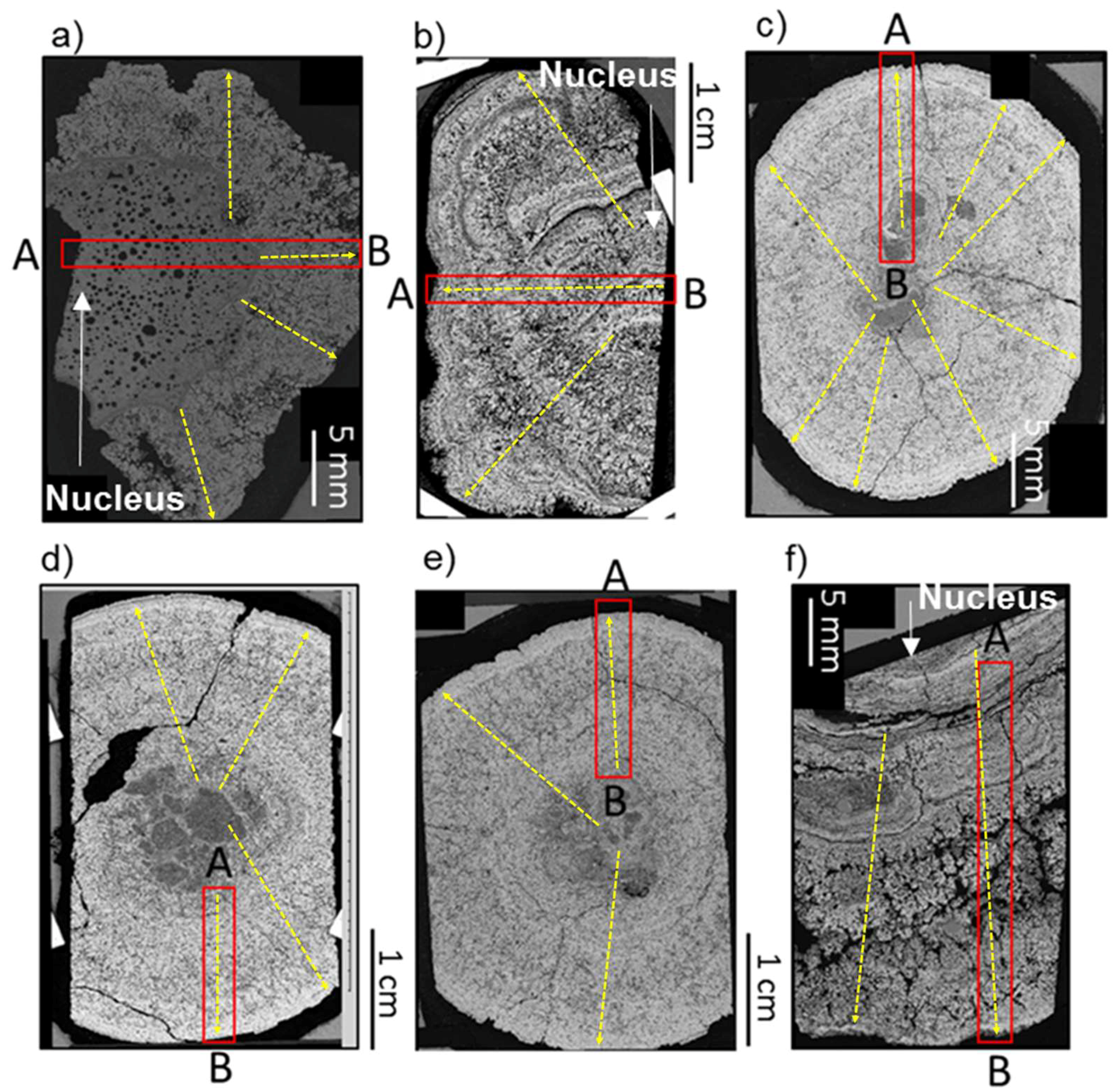
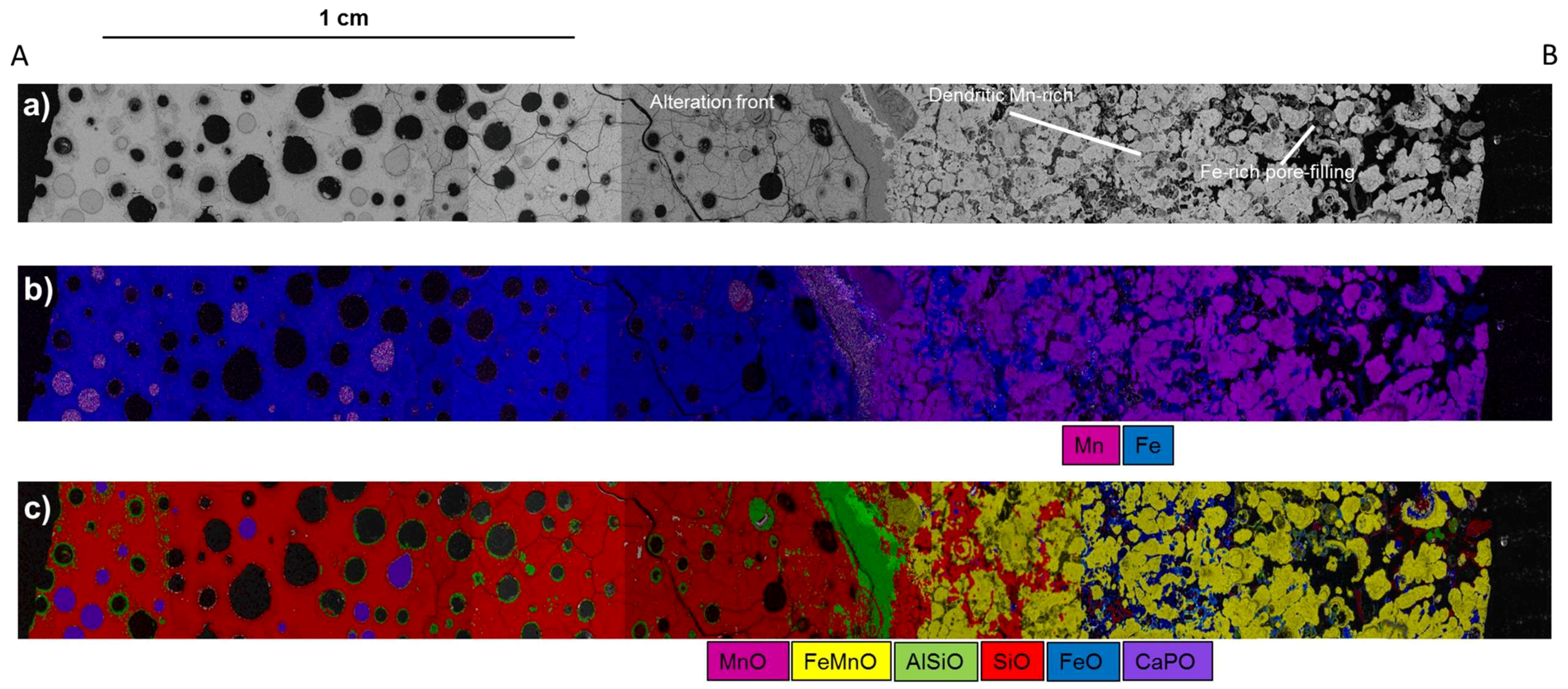
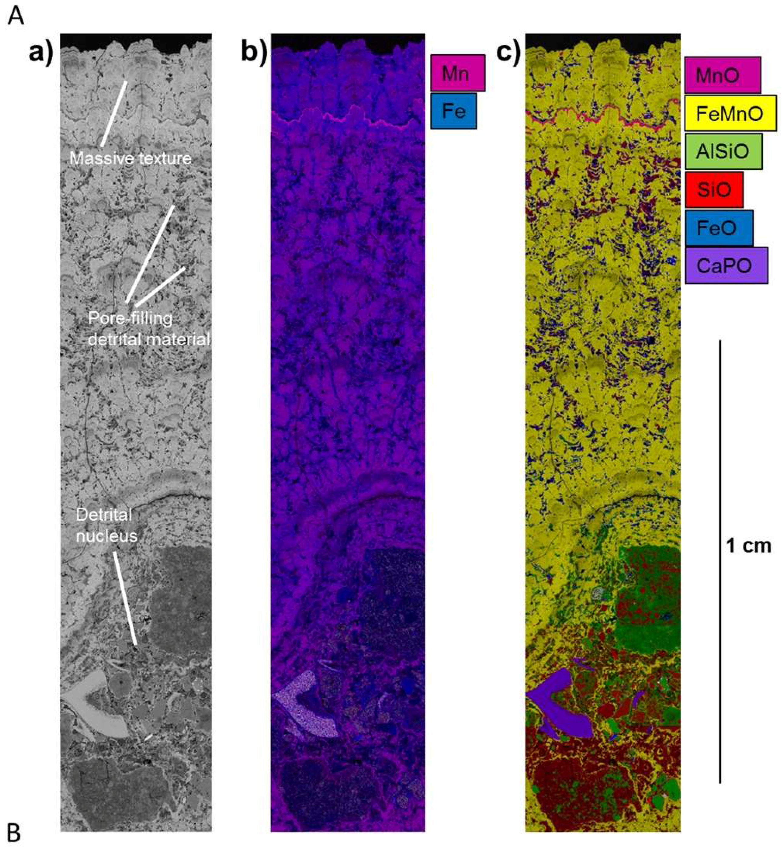
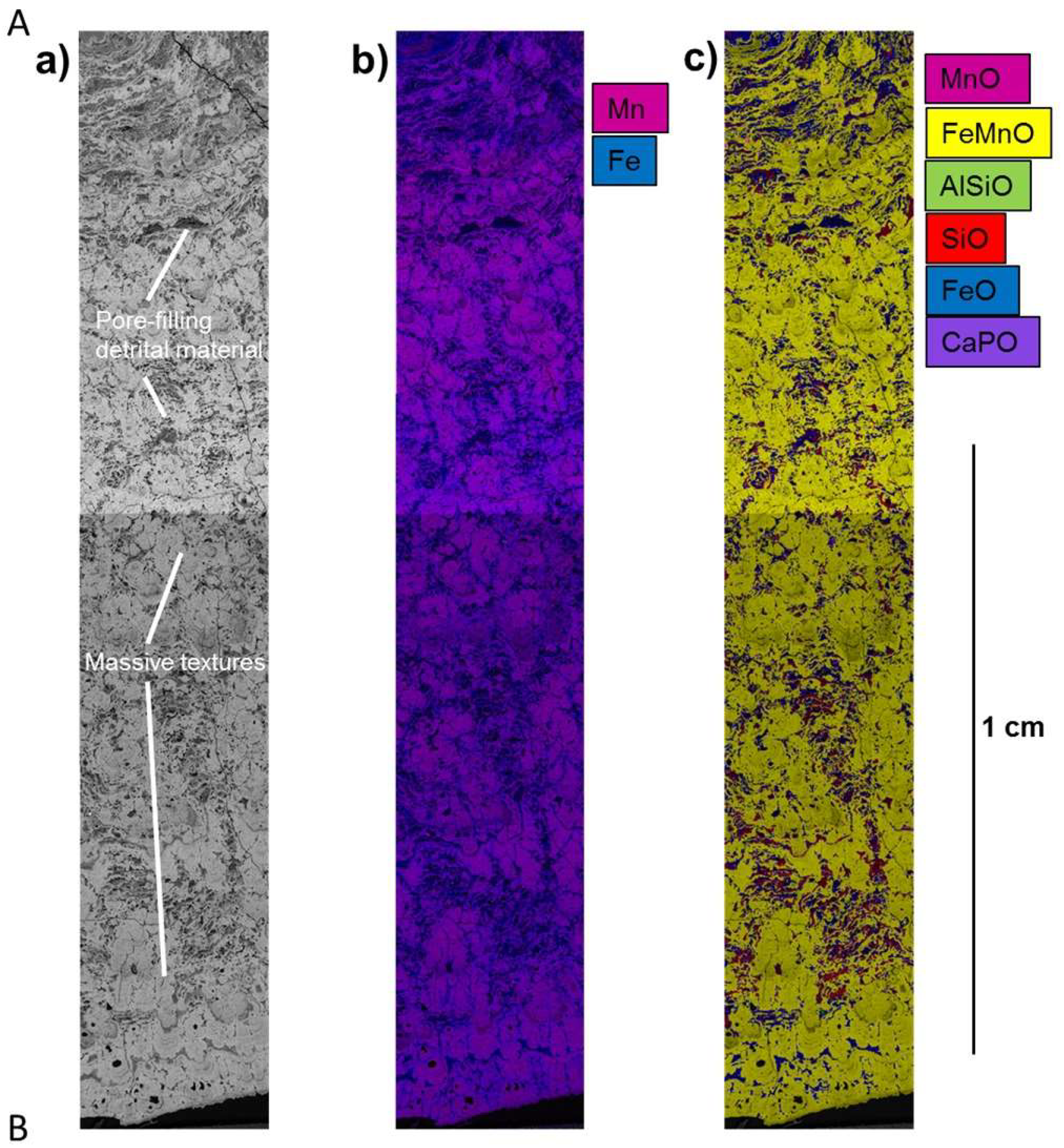
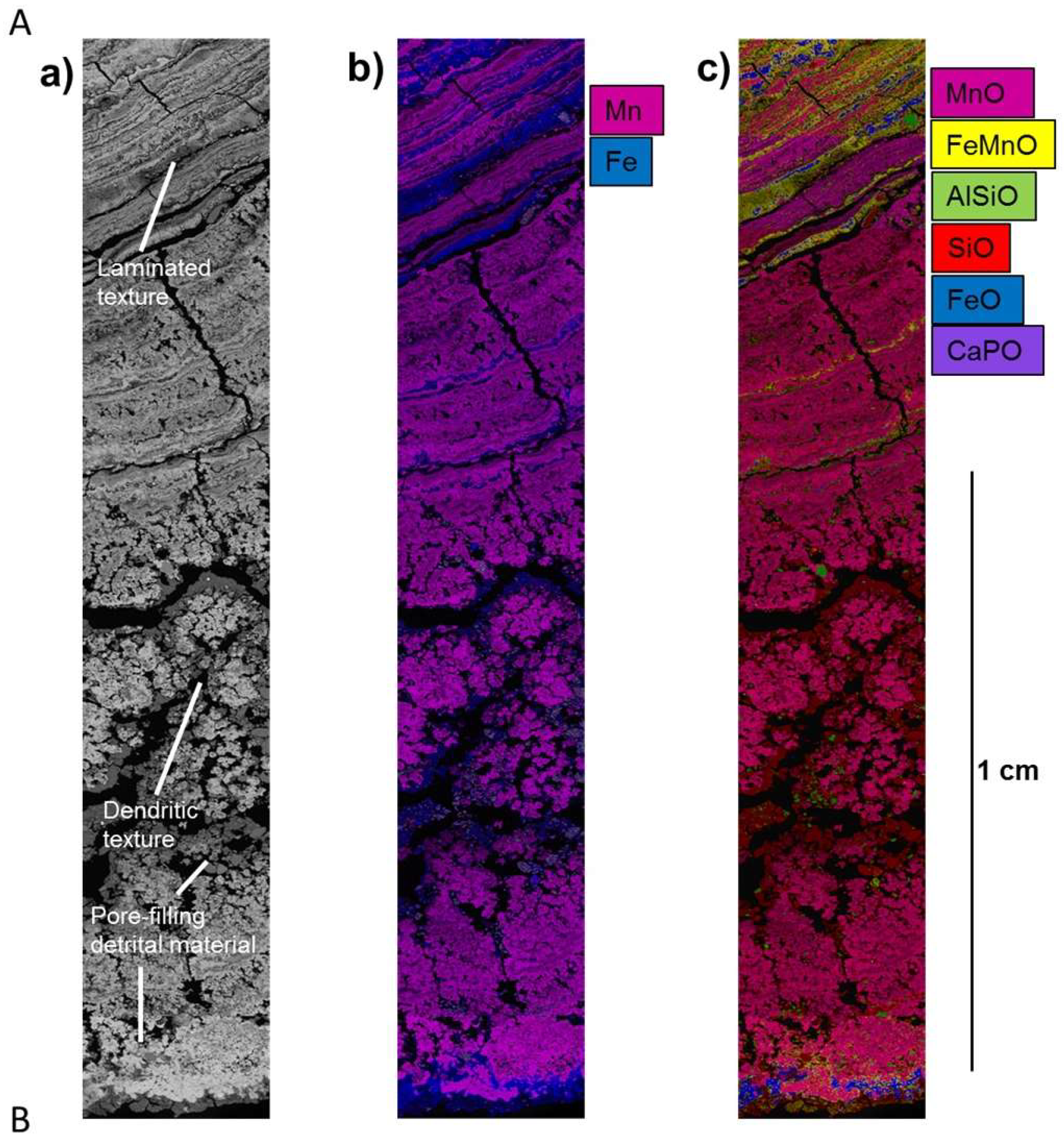
4.1. Internal Structure of Nodules and Crust

Backscatter images (Figure 2, Figure 3, Figure 4, Figure 5, Figure 6, Figure 7 and Figure 8a) reveal that the nodules and crust have layered growth patterns which tend to be concentric in the smaller nodules (EATL N4, NAP N4, and RC12-192), but more complex and irregular in the larger nodules and the crust. Individual layers are distinguished by differences in reflectivity, with dark, low reflectivity layers alternating with bright, highly-reflective layers. Elemental mapping (Figure 2, Figure 3, Figure 4, Figure 5, Figure 6, Figure 7 and Figure 8b,c) was used to map the distribution of major elements throughout the nodule structure.

Nodule JC120-104 (Figure 2 and Figure 3) is characterised by an irregular distribution of layers that reveals a complex growth history. There are at least two generations of nodule growth (Figure 1b), and the central part of the nodule is formed from a fragment of an older nodule over which new layers have precipitated. Both the older nodule and the newer layers are characterised by dendritic Mn-rich oxides that appear bright in the backscatter image, surrounded by pore spaces that are generally filled with aluminosilicate or Ca-phosphate detrital material. Occasional parallel layers of Mn-Fe oxides that appear dark in the backscatter image alternate with the dendritic structure. These are often intercalated with aluminosilicate material. Aluminosilicate material can also found filling cracks within the nodule structure.

The crust sample (EW9602-09RD; Figure 4) is composed of a large porous basaltic glass fragment on which finely-crystallised Fe-Mn oxides have precipitated in a dendritic pattern. Some of the pores in the basaltic glass are empty and rimmed by aluminosilicate material that is likely a product of alteration. Other pores are filled in with Ca-phosphate. At the contact between the glass and the Fe-Mn crust, there is an Al-rich alteration front (Figure 4c). The Fe-Mn oxides beyond the alteration front are finely crystalline and appear bright in backscatter images (Figure 4a), and Fe-oxides (usually in the form of aluminosilicates) can be observed filling the pore spaces (Figure 4c). Sub-angular aluminosilicate clasts are common in the pore spaces towards the outer part of the crust structure.

Nodule samples RC12-192GS (Figure 5), EATL N4 (Figure 6), and NAP N4 (Figure 7) have similar morphological and chemical characteristics. They are composed by finely-crystallised Fe-Mn oxides that appear bright in backscatter images, have a dense, massive structure and surround a nucleus composed of multiple silicate-rich (e.g., Figure 5c), aluminosilicate (Figure 5, Figure 6, and Figure 7c) or Ca-phosphate (Figure 5, Figure 6, and Figure 7c) clasts. Fe-rich aluminosilicate material that appears dark in backscatter images can be found in pores and cracks throughout the nodule structure. Thin Mn-oxide rich layers that appear bright in backscatter images are also sparsely present in the nodules (Figure 5 and Figure 6c).

Nodule sample PSh-125.29(1) (Figure 8) is characterised by large dendritic Mn-rich structures infilled with angular aluminosilicate detrital material. The Mn-rich oxides overlap the nucleus, and alternate with Fe-Mn oxide-rich layers that appear dark in backscatter images (Figure 8c). Fe oxides occur in discrete dark layers both towards the edge of the nodule and towards the nucleus.

4.2. Chemical Composition of Internal Layers

Laser ablation analyses shows that nodule layers that appear dark in backscatter images have relatively low Mn/Fe ratios (<3) and low Ni + Cu (<1.5 wt %), and relatively high concentrations of Co (>0.2 wt %) and REY (>1600 ppm). By contrast, layers that appear bright in backscatter images have high Mn/Fe ratios (>3) and high Ni + Cu (>1 wt %), but low Co (<0.2 wt %) and low REY (<1600 ppm) (Table 2 and Table 3). Average metal concentrations in the layers are in general agreement with bulk data from the same locations reported by other authors (Table 2 and Table 3).

The crust sample has highest concentrations of both Mn (~42 wt %) and Fe (~24 wt %), and there is little variation in the Mn/Fe ratio of individual layers, ranging from ~1.3 to ~2.8. The crust has relatively high concentrations of Co (~0.7–3.7 wt %), Ti (~1.7–2.1 wt %), V (~840–1170 ppm), and Ba (~2570–2900 ppm). The nodule from the CCFZ (JC120-104) has the highest average Mn/Fe ratio (~8.8); this nodule incorporates layers that have extremely high Mn/Fe, up to ~80, as well as layers with lower Mn/Fe, ~1.6. Ni, Cu, and Zn also show high concentrations in the high Mn/Fe layers (~1.10 wt %, ~0.90 wt % and ~3740 ppm, respectively), and lower concentrations in the low Mn/Fe layers (~0.4 wt %, 0.18 wt % and ~617 ppm).

South Pacific nodule sample RC12-192GS mainly consists of low Mn/Fe layers (~1.5–1.7), although a few layers have slightly higher Mn/Fe (up to ~6). Layers with higher Mn/Fe also tend to have high Ni + Cu and Zn (~3.14 wt % and ~1310 ppm, respectively), whereas the layers with low Mn/Fe tend to have higher Co (~0.38 wt %), Ti (~0.7–1.2 wt %), and Ba (~1290–3510 ppm).

Atlantic nodules NAP N4 and EATL N4 have relatively low average Mn/Fe, ~1.2 and ~1.4, respectively. Some layers are moderately enriched in Mn relative to Fe, with Mn/Fe of ~8.9. These nodules have relatively high concentrations of Co (~0.6–0.5 wt %), Ti (~1.1–1 wt %), V (~721–680 ppm), Th (~140–130 ppm), and U (11.4–10.4 ppm).

The Arctic nodule PSh-125.29(1) has a moderate Mn content of ~23 wt %, but relatively low Fe (~7.5 wt %). This nodule has relatively low concentrations of other metals, with Co, Ni, and Cu concentrations of ~0.01 wt %, Ti = ~0.1 wt %, V = ~228 ppm, Zn = ~50 ppm, Ba = ~770 ppm, Th = ~6.3 ppm, and U = ~4.7 ppm. Some layers have relatively high Mn/Fe (~10), and these tend to have higher concentrations of Co + Ni + Cu.

Nodules from the Atlantic Ocean, EATL N4, and NAP N4 that have relatively low Mn/Fe, have the highest concentrations of REY, with average ΣREY concentrations of, respectively, ~3360 and ~3880 ppm. ΣREY concentrations in the Pacific nodule RC12-192GS and crust EW9602-09RD are lower, ~2670 and ~2500 ppm, respectively, whereas the Pacific nodule that has highest Mn/Fe (JC120-104) has much lower ΣREY (~990 ppm). The Arctic nodule PSh-125.29(1) has extremely low ΣREY (~123 ppm). Most of the individual nodule layers have positive Ce anomalies, whereas high Mn/Fe layers in nodule JC120-104 and most layers in nodule PSh-125.29(1) have negative Ce anomalies. All layers are generally depleted in the LREE relative to the HREE, especially in JC120-104 (LREE/HREE = 0.46).

4.3. Factor Analysis

To assess the controls on the chemical composition of the nodules and crust, the elemental data were subjected to statistical factor analysis [38] using the RStudio Inc. Varimax rotation scheme with Kaiser normalisation (RStudio.Inc., Boston, MA, USA). The results of this analysis are shown in Table 4, and in Table A1, Table A2, Table A3, Table A4, Table A5 and Table A6 in Appendix A. Most of the total variance in the chemical composition within nodule JC120-104 and the crust (EW9602-09RD) can be accounted for by five factors, and most of the variance in nodules RC12-192GS, EATL N4 and NAP N4 can be accounted for by four factors. The variance in the chemical composition of the nodule from the Arctic (PSh-125.29(1)) is mainly accounted for by three factors.

Factor 1 is the most important control on REY concentrations in all samples (excluding Ce in the crust and nodules JC120-104 and PSh-125.29(1)), and Ti, V, Fe, and Co in Atlantic nodules NAP N4 and EATL N4, and the South Pacific nodule RC12-192GS. In the Arctic nodule this factor controls V, Fe, and the REY. Factor 1 accounts for 50–77% of the total variance of the samples. In most of the samples it has negative loadings for Mn, Ni, Cu, and Zn. This factor likely represents the hydrogenous Fe-Mn-(oxyhydr)oxide fraction of the Atlantic and South Pacific nodules (represented by FeMnO in the elemental maps, Figure 3, Figure 4, Figure 5, Figure 6, Figure 7 and Figure 8) and identified as Fraction 3 by [39]. In the Arctic nodule it likely represents detrital aluminosilicate material (SiO in Figure 8) and is identified as Fraction 4 by [39]. In nodule JC120-104 and the crust it most likely represents a Ca-rich phosphate (CaP in Figure 3) in association with Fe-(oxyhydr)oxides, although this cannot be confirmed as no Ca or P data were acquired.

Factor 2 controls Mn, Ni, Cu, and Zn in the Atlantic nodules NAP N4 and EATL N4, the South Pacific nodule RC12-192GS, and the Arctic nodule PSh-125.29(1). In these samples it has negative loadings for Fe, Cr, and Th. In sample JC120-104 this factor controls Fe, Ce, Th, and U, and it has significant negative loadings for Mn and Zn. In the crust this factor controls Ti, V, Fe, Co, Ba, Ce, U, and partially Mn. Factor 2 most likely represents the Mn-rich diagenetic fraction of the nodules (identified as MnO in Figure 3, Figure 4, Figure 5, Figure 6, Figure 7 and Figure 8) and is similar to Fraction 2 reported by [39]. This factor may also be associated with Fe-oxides in nodule JC120-104 (FeO in Figure 3). In the crust this factor most likely represents an additional hydrogenous phase (FeMnO in Figure 4) and is denoted Fraction 3 in [39]. This factor accounts for the 13–24% of the total variance in the chemical composition of all of the ferromanganese deposits sampled in this study.

Factor 3 controls Ti, V, Cr, and Fe in most of the nodules, and Co, Ti, Nd, Gd, Dy, and U in the crust. This factor likely represents the material (AlSiO in Figure 3, Figure 4, Figure 5, Figure 6, Figure 7 and Figure 8), and it accounts for 4–10% of the total variance in the chemical composition. This fraction is part of the residual group identified by [39] as Fraction 4.

Factor 4 controls Co in the Atlantic nodule EATL N4, Ni, and Cu in JC120-104 and Mn, Ni, Cu, and Zn in the crust, but it does not have a significant loading in any of the other samples. It accounts for the 1–6% of the total variance. The element distribution suggest that Factor 4 represents an additional hydrogenous oxide in the nodules (likely included in the FeMnO phase in Figure 3, Figure 4, Figure 5, Figure 6, Figure 7 and Figure 8, and part of Fraction 3 in [39], and a pure diagenetic Mn-oxide fraction in the crust (MnO in Figure 4, that is identified as Fraction 2 in [39].

Factor 5 is only present in the crust sample EW9602-09RD, and it only shows a significant loading for Mn in the crust and for Co in the CCFZ nodule JC120-104, which might be indicative of additional minor amounts of Mn-Fe oxides. It accounts for 5% of the total sample variance.

5. Discussion

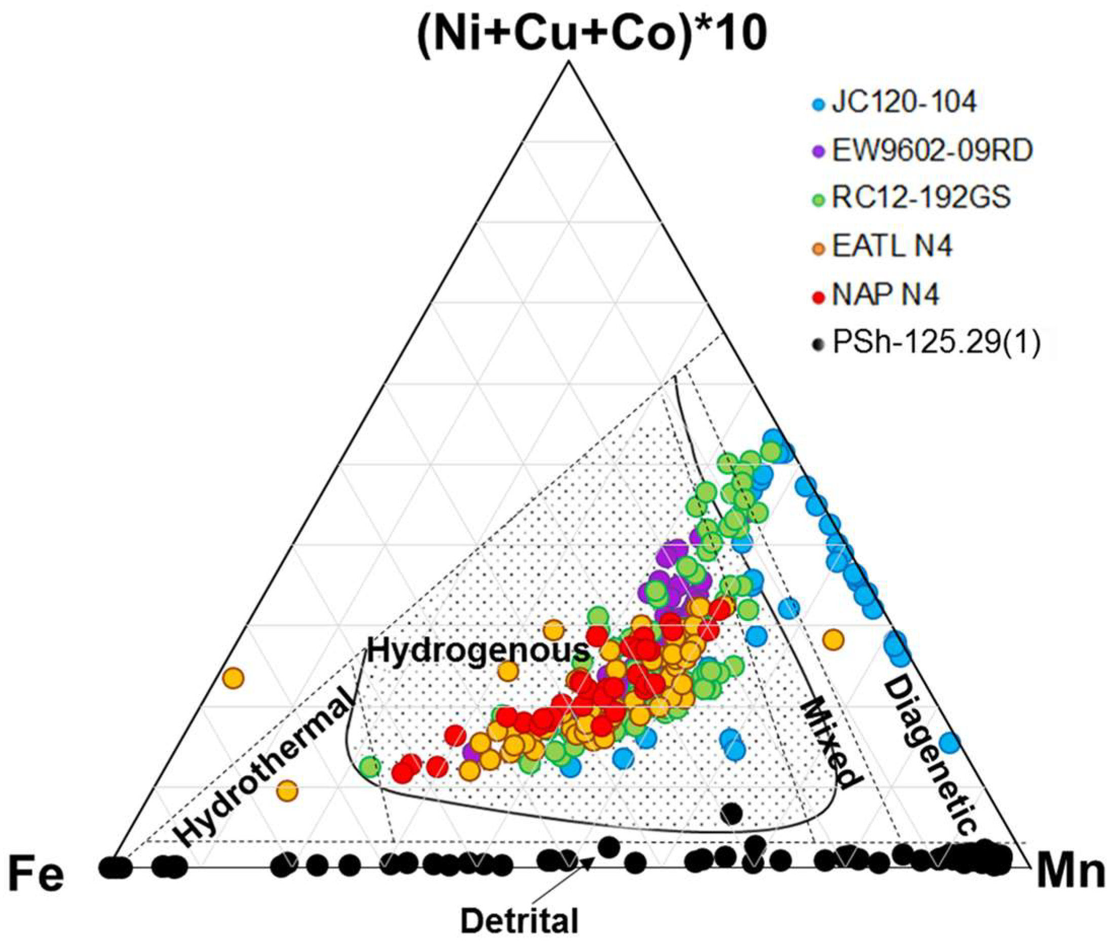
5.1. Genesis of Deep-Sea Ferromanganese Deposits

SEM analyses reveals that the internal structure of deep-sea ferromanganese deposits is highly heterogeneous. In turn, our LA-ICP-MS analyses indicate that the chemical composition of the crust and nodules is also heterogeneous, and factor analysis shows that individual deposits can acquire metals and REYs from a variety of different sources, including seawater, sediment pore waters, and aluminosilicate material. Based on the relative abundances of Mn, Fe, and Ni + Cu + Co [40], the ferromanganese crust and nodules from the Atlantic Ocean mainly acquire metals from seawater, whereas different layers within the nodules from the Pacific Ocean acquire metals either from seawater or sediment pore waters (Figure 9), which would not be apparent from measurements of their bulk chemical composition.

High-resolution mapping of individual layers within nodules from the German license area E1 in the easternmost part of the CCFZ also reveals the presence of both dense, dark layers with low average Mn/Fe (1.8) and low average Ni + Cu (0.81 wt %), and bright dendritic layers with high average Mn/Fe (96) and high Ni + Cu (~4 wt %) [18]. The former were referred to as “layer type 1” and were attributed to hydrogenetic precipitation from oxic waters, whereas the latter were referred to as “layer type 2” and attributed to metal precipitation from sub-oxic pore waters. Most of the nodule and crust layers analysed in this study have relatively low Mn/Fe (<~3; Table 2) and the only layers that have very high Mn/Fe (up to 80.4) come from the nodule sample JC120-104, which is also from the CCFZ. Thin microlayers in Atlantic nodules NAP N4 and EATL N4 and in the South Pacific nodule RC12-192GS have intermediate Mn/Fe values of between 3 and 10 and intermediate Ni + Cu concentrations of 2–3 wt %. These microlayers appear bright in the backscatter images shown in Figure 5, Figure 6 and Figure 7. Although many authors have observed “mixed” hydrogenetic-diagenetic signals, they are typically attributed to the mixing of type 1 and type 2 layers during bulk analysis [18]; however, we note that some of the layers with intermediate Mn/Fe values have higher Cu + Ni, which suggests that these layers form from an oxic diagenetic, rather than a hydrogenous, source.

REY analyses may also be useful for assessing the principal mode of formation of different layers [12,41,42,43]. REY distribution patterns for different layers within the Atlantic nodules are relatively homogeneous, with strong positive Ce anomalies (~2.5–4), and enrichment of Ho with respect to Y (Figure 10). This pattern is typical for surface complexation of REY from ambient seawater and subsequent hydrogenetic precipitation [10,20,21,26,43]. The crust sample also has a positive Ce anomaly (2.31–4.45), but it is more strongly enriched in the HREE relative to the LREE compared to the Atlantic nodules. This is characteristic of hydrogenetic crusts that are phosphatised [44], consistent with our SEM observations of the presence of Ca-phosphate filled cavities within the crust structure (Figure 4c).

Layers that have relatively high Mn/Fe (principally those within the nodule from the CCFZ, sample JC120-104) by contrast have negative Ce anomalies (~0.75 compared to ~1.5 for layers with low Mn/Fe), as well as lower REY concentrations (~230 vs. ~1620 ppm for layers with low Mn/Fe). Early diagenesis of organic material mobilises Mn and the trivalent REY, but not Ce⁴⁺ [12,45,46]. Mn and the trivalent REY subsequently precipitate at the sub-oxic/oxic interface, so Ce⁴⁺ is depleted relative to the trivalent REEs in ferromanganese precipitates. The lower REY content of these layers is likely due to the relatively fast nature of diagenetic precipitation [10,46], as the REY are complexed in seawater and REY complexes are scavenged very slowly [12,20,26]. Mn deposit in slow-precipitating, colloidal related elements, such as the REY. Additionally, diagenesis can induce the dissolution of Fe-Mn-(oxyhydr)oxides, releasing associated REY to sediment pore waters [42].

Plots of the Ce anomaly vs. Y/Ho and Nd concentration (Figure 11) support the REY distributions. The only layers that have a diagenetic signature are from the Arctic nodule and some of those from the CCFZ nodule; all of the other layers represents hydrogenetic precipitates. As our high-resolution data clearly distinguishes hydrogenous and diagenetic precipitates, we can better assess their relative growth rates based on Co content [48]:

Growth Rate = 0.68/(Co_n)^1.67,

(1)

where Co_n = Co × 50/Fe + Mn, with Co, Fe and Mn in wt %. This method does not account for any hiatuses in precipitation of Co (e.g., [48]) and, therefore, only provides a minimum age. Bearing this in mind, our data indicate that the hydrogenetic layers have relatively slow growth rates (~1–2 mm/Ma), whereas the diagenetic layers form much more rapidly (up to ~10–17 mm/Ma in the nodule JC120-104). This is consistent with results of other studies based on bulk compositions (e.g., [9]).

A model summarising the different modes of nodule formation revealed in this study is shown in Figure 12. The greater diagenetic component of the nodule from the CCFZ in comparison with the other deposits indicates that conditions in surface sediments must have been sub-oxic for sustained periods at this site during nodule formation. The oxygen penetration depth (OPD) into sediments in the CCFZ at the present day is ~1 m (Table 1). However, in the past, at the time the nodule started to form (~17 Ma, based on its size and growth rate), this site was located closer to the equator, which is a zone of high primary productivity. The higher availability of organic matter in the bottom sediments at this time suggests that the oxic/sub-oxic boundary within the sediments was located closer to the seafloor, facilitating nodule growth by diagenetic processes (Figure 12a). By contrast, the typical oxygen penetration depth (OPD) in the deep North Atlantic Ocean at the present day is much deeper, ~18 m [27], and bottom waters are highly oxygenated [43]. The OPD in the South Pacific abyssal plain, close to the location of nodule sample RC12-192GS and crust sample EW9602-09RD, is also deep (up to 75 m; [23]) due to low primary productivity in the South Pacific Gyre. Hence, nodules and crusts that form on sediments that have a low organic carbon content tend to have a hydrogenous source, whereas nodules that rest on sediments with a relatively shallow OPD also contain a diagenetic signature (Figure 12).

The transition metal and REY composition of the Arctic nodule is clearly different from the other nodules and the crust (Figure 9 and Figure 10). This nodule has exceptionally low Ni + Cu + Co and very variable Mn and Fe, similar to the bulk composition of nodules from the Kara Sea [36]. This type of composition is usually attributed to a hydrothermal source [40], but the nodules have negative, rather than positive, Y anomalies (Figure 10) that preclude hydrothermal input [12]. Additionally, the REY distribution pattern and REY concentration of the Arctic nodules is rather similar to shale (Figure 10), consistent with statistical element associations (Table 3) that indicate that the principal source of the REY is the input of detrital material. For this reason, we have delimited a new field for detritally-sourced nodules on Figure 9. Mn/Fe ratios within individual nodule layers are highly variable (0.74–10), and much higher than NASC (0.016; [47]). Together with negative Ce anomalies (Figure 9 and Figure 10) this is strong evidence for diagenetic precipitation from sub-oxic pore waters [12]. Consequently, nodules are only found in those parts of the Kara Sea that host a thin layer of oxic sediments (Figure 12), and they are absent in anoxic sediments presumably because Mn (and Fe) oxyhydroxides cannot precipitate [30]. In addition, the Arctic nodule has an extremely high growth rate (Equation (1); up to ~8080 mm/Ma), similar to that estimated for shallow water nodules from the Gulf of Cadiz (~1400–5000 mm/Ma; [5]). Thus, dilution of the authigenic phases by detrital material, combined with high nodule growth rates and rapid burial rates [4] preclude significant enrichment in Ni + Cu + Co and the REY; models for the genesis of nodules based on geochemical relationships observed in deep-sea settings cannot, therefore, be applied to nodules that form in shallow waters.

5.2. Controls on the Resource Potential of Deep-Sea Ferromanganese Deposits

The economic resource of ferromanganese deposits is mainly based on their high content of Ni, Co, and Cu, with a growing interest in their potential as a REY resource.

Our study nevertheless reveals that the metal content of ferromanganese deposits can be highly variable, depending on their environmental setting. Table 5 provides an estimate of metal resource potential based on the average of all of our LA-ICP-MS analyses. Overall, dominantly hydrogenetic deposits tend to offer a better resource potential for Co and REY, while dominantly diagenetic deposits have higher concentrations of Ni and Cu. Shallow-water nodules from the Kara Sea do not contain high quantities of any of these metals, and estimated resources of Ni and Cu are much lower than the global annual consumption (Table 5).

Nodules from the Northwest Atlantic basin could supply significant quantities of Co (~up to 72 × 10⁵ T) and REY (~up to 38 × 10⁵ T), representing ~90 times the current global annual consumption of Co and ~36 times that of the REY (Table 5). As hydrogenetic nodules tend to be smaller, the nodule density is lower, so only very large fields of hydrogenetic nodules are likely to represent a viable resource. As discussed in Section 2, large nodule fields are, however, scarce in the Atlantic Oceans as they are confined to relatively small, deep basins because sedimentation rates are too high in the rest of the ocean to support nodule formation [20]. On the other hand, lower sedimentation rates and a shallower carbonate compensation depth (CCD) makes nodule-rich deep basins in the Pacific more common and extensive. For these reasons, large-sized diagenetic nodules from the CCFZ provide a similar metal tonnage to hydrogenetic nodules (up to ~68 × 10⁵ T of Co, and up to ~34 × 10⁵ T of REY), even though they are less enriched in Co and REY. Similarly, the high quantities of ferromanganese crusts in the large Southwestern Pacific seamount province (up to ~75 kg/m², [29]) provide up to ~14.2 × 10⁵ T of Co (~16 times the global annual demand) and ~2.3 × 10⁵ T of REY (~2 times the global annual demand), even though the crusts are only found on the top of seamounts that have a maximum surface area of ~1200 km².

The diagenetically-influenced nodules from the CCFZ have the potential to yield the highest tonnages in Ni and Cu, up to ~376 and ~304 × 10⁵ T, respectively (Table 5), which represents ~0.03 times the global annual consumption of Ni and ~1.35 times that of Cu. In comparison, the amounts of Cu and Ni contained in hydrogenetic deposits are ca. one order of magnitude lower.

6. Conclusions

Analyses of the structure and chemical composition within individual nodules and crusts reveal great internal variability. Nodules from the Atlantic Ocean, and the ferromanganese crust sample, tend to consist of layers of Fe-Mn-rich oxides with relatively low Mn/Fe (<3) that precipitate from oxic seawater. These nodules are enriched in ΣREY, Fe, and Co, and they grow only slowly (~1 mm/Ma). The crust sample has experienced diagenetic phosphatization. Large nodules from the CCFZ in the Pacific Ocean also contain layers that have much higher Mn/Fe (up to ~60) and Cu, Ni, and Zn, that precipitate from sub-oxic sediment pore waters. These layers grow much faster (~7 mm/Ma) compared to the layers that have low Mn/Fe (~1–2 mm/Ma). Nodules from the shallow Arctic Ocean have highly variable textures, with high concentrations of detrital material and relatively low concentrations of transition metals and ΣREY. The Arctic nodules are extremely fast-growing (~500 mm/Ma).

The mode of genesis of ferromanganese deposits, as well as their growth rate and the oxygen penetration depth of their host sediments, all affect the final resource potential. Although hydrogenetic deposits are generally better resources of Co and the REY, diagenetic deposits have higher quantities of Ni and Cu, and they also tend to have higher nodule densities because they grow more quickly. Arctic nodules are a poor resource because they have a high detrital component. Deep sea nodules and ferromanganese crusts contain significant quantities of ΣREY and Co with respect to the global annual demand, but are less important resources of Ni and Cu.

Author Contributions

Doug Connelly and Natalia Shulga provided some of the samples for this work; Amaya Menendez, Rachael James, and Steve Roberts conceived and designed the experiments; Amaya Menendez performed the experiments, analysed the data, and wrote the paper; and Rachael James substantially revised the work. The authors have approved the submitted version and agree to be personally accountable for the author’s own contributions and for ensuring that questions related to the accuracy or integrity of any part of the work, even ones in which the author was not personally involved, are appropriately investigated, resolved, and documented in the literature.

Acknowledgments

This work was funded by the European Union Seventh Framework Programme (FP7/2007–2013) under the MIDAS project, grant agreement no. 603418. The authors wish to thank Kate Peel, Matthew Cooper, J. Andy Milton, and Richard Pearce (University of Southampton) for training and technical support for geochemical analyses.

Conflicts of Interest

The authors declare no conflict of interest. The founding sponsors had no role in the design of the study; in the collection, analyses, or interpretation of data; in the writing of the manuscript; or in the decision to publish the results.

Appendix A

Varimax rotated correlation matrices for samples in this study are shown. Numbers in bold denote elements that appear to have a significant correlation (p < 0.05).

Table A1. Correlation coefficients between elements in sample JC120-104. Significant (p < 0.05) correlations are highlighted in bold.

JC120−104
	Ti	V	Cr	Mn	Fe	Co	Ni	Cu	Zn	Ba	La	Ce	Pr	Nd	Sm	Eu	Gd	Tb	Dy	Y	Ho	Er	Tm	Yb	Lu	Th	U
Ti	1.00
V	0.48	1.00
Cr	0.05	−0.09	1.00
Mn	−0.84	−0.13	−0.17	1.00
Fe	0.91	0.52	−0.01	−0.82	1.00
Co	0.12	0.36	0.19	−0.14	0.09	1.00
Ni	−0.56	−0.54	0.04	0.39	−0.62	−0.13	1.00
Cu	−0.62	−0.56	0.01	0.54	−0.70	−0.12	0.85	1.00
Zn	−0.79	−0.17	−0.24	0.92	−0.71	−0.32	0.26	0.36	1.00
Ba	0.22	0.69	0.09	0.02	0.18	0.56	−0.23	−0.14	−0.19	1.00
La	0.40	0.46	−0.17	−0.41	0.50	0.42	−0.45	−0.45	−0.37	0.26	1.00
Ce	0.95	0.60	−0.06	−0.80	0.95	0.22	−0.61	−0.68	−0.74	0.27	0.55	1.00
Pr	0.23	0.32	−0.13	−0.28	0.30	0.44	−0.31	−0.30	−0.26	0.20	0.97	0.36	1.00
Nd	0.20	0.31	−0.13	−0.26	0.27	0.44	−0.30	−0.29	−0.25	0.20	0.96	0.34	1.00	1.00
Sm	0.17	0.29	−0.12	−0.23	0.23	0.44	−0.28	−0.27	−0.22	0.18	0.95	0.30	1.00	1.00	1.00
Eu	0.17	0.28	−0.12	−0.23	0.22	0.44	−0.27	−0.26	−0.22	0.18	0.95	0.29	1.00	1.00	1.00	1.00
Gd	0.19	0.28	−0.12	−0.26	0.25	0.44	−0.29	−0.28	−0.24	0.17	0.95	0.32	1.00	1.00	1.00	1.00	1.00
Tb	0.21	0.29	−0.12	−0.27	0.26	0.43	−0.29	−0.29	−0.25	0.18	0.96	0.34	1.00	1.00	1.00	1.00	1.00	1.00
Dy	0.22	0.30	−0.13	−0.28	0.28	0.43	−0.30	−0.30	−0.27	0.18	0.96	0.35	1.00	1.00	1.00	1.00	1.00	1.00	1.00
Y	0.10	0.15	−0.10	−0.20	0.13	0.43	−0.19	−0.17	−0.21	0.11	0.90	0.21	0.98	0.98	0.99	0.99	0.99	0.98	0.98	1.00
Ho	0.23	0.29	−0.13	−0.29	0.28	0.43	−0.30	−0.29	−0.28	0.18	0.96	0.35	1.00	1.00	1.00	1.00	1.00	1.00	1.00	0.98	1.00
Er	0.24	0.29	−0.13	−0.30	0.28	0.43	−0.29	−0.29	−0.29	0.18	0.96	0.36	1.00	1.00	0.99	1.00	1.00	1.00	1.00	0.98	1.00	1.00
Tm	0.26	0.30	−0.13	−0.31	0.30	0.43	−0.30	−0.30	−0.30	0.19	0.96	0.38	0.99	0.99	0.99	0.99	0.99	1.00	1.00	0.98	1.00	1.00	1.00
Yb	0.27	0.30	−0.13	−0.31	0.30	0.43	−0.30	−0.30	−0.31	0.19	0.96	0.38	0.99	0.99	0.99	0.99	0.99	1.00	1.00	0.98	1.00	1.00	1.00	1.00
Lu	0.28	0.31	−0.13	−0.33	0.32	0.43	−0.31	−0.31	−0.32	0.19	0.96	0.40	0.99	0.99	0.99	0.99	0.99	0.99	1.00	0.98	1.00	1.00	1.00	1.00	1.00
Th	0.84	0.45	0.00	−0.80	0.86	0.24	−0.59	−0.62	−0.73	0.16	0.75	0.88	0.63	0.61	0.58	0.58	0.60	0.61	0.62	0.52	0.63	0.63	0.65	0.65	0.67	1.00
U	0.88	0.47	−0.10	−0.75	0.88	0.14	−0.68	−0.66	−0.72	0.22	0.48	0.91	0.31	0.28	0.24	0.24	0.27	0.28	0.30	0.18	0.30	0.31	0.33	0.33	0.35	0.84	1.00

Table A2. Correlation coefficients between elements in sample EW9602-09RD. Significant (p < 0.05) correlations are highlighted in bold.

EW9602-09RD
	Ti	V	Cr	Mn	Fe	Co	Ni	Cu	Zn	Ba	La	Ce	Pr	Nd	Sm	Eu	Gd	Tb	Dy	Y	Ho	Er	Tm	Yb	Lu	Th	U
Ti	1.00
V	0.55	1.00
Cr	0.001	−0.03	1.00
Mn	0.38	0.45	−0.59	1.00
Fe	0.19	0.63	0.06	−0.002	1.00
Co	−0.33	−0.41	−0.46	0.62	−0.26	1.00
Ni	−0.20	−0.34	−0.30	0.46	−0.65	0.12	1.00
Cu	0.56	0.37	0.08	−0.05	−0.25	−0.40	0.58	1.00
Zn	0.26	0.55	0.30	−0.10	0.36	−0.03	−0.13	0.21	1.00
Ba	0.28	0.66	0.13	0.07	0.88	−0.25	−0.48	−0.09	0.54	1.00
La	0.39	0.81	−0.30	0.43	0.62	0.39	−0.40	−0.62	0.22	0.54	1.00
Ce	0.42	0.69	0.04	0.12	0.74	0.13	−0.63	−0.43	0.34	0.74	0.68	1.00
Pr	0.48	0.80	−0.22	0.40	0.40	0.58	−0.33	−0.67	0.33	0.36	0.92	0.56	1.00
Nd	0.50	0.79	−0.19	0.38	0.37	0.57	−0.33	−0.68	0.33	0.35	0.91	0.55	1.00	1.00
Sm	0.50	0.75	−0.14	0.32	0.29	0.59	−0.30	−0.69	0.37	0.29	0.83	0.49	0.98	0.99	1.00
Eu	0.54	0.78	−0.12	0.34	0.35	0.57	−0.32	−0.67	0.39	0.35	0.86	0.54	0.98	0.99	0.99	1.00
Gd	0.57	0.76	−0.10	0.32	0.32	0.56	−0.32	−0.69	0.37	0.33	0.84	0.54	0.96	0.98	0.99	0.99	1.00
Tb	0.60	0.78	−0.08	0.34	0.31	0.56	−0.29	−0.65	0.39	0.34	0.83	0.53	0.95	0.97	0.98	0.99	0.99	1.00
Dy	0.65	0.80	−0.09	0.37	0.35	0.56	−0.31	−0.66	0.38	0.38	0.84	0.57	0.95	0.96	0.96	0.98	0.99	0.99	1.00
Y	0.69	0.80	0.08	0.27	0.53	0.31	−0.42	−0.58	0.40	0.58	0.79	0.65	0.82	0.84	0.82	0.86	0.88	0.89	0.93	1.00
Ho	0.70	0.82	−0.06	0.38	0.40	0.51	−0.33	−0.63	0.37	0.45	0.84	0.60	0.91	0.93	0.92	0.94	0.96	0.97	0.99	0.97	1.00
Er	0.74	0.84	−0.03	0.40	0.44	0.49	−0.34	−0.60	0.38	0.50	0.83	0.62	0.89	0.90	0.89	0.91	0.93	0.95	0.97	0.97	0.99	1.00
Tm	0.75	0.85	−0.01	0.40	0.45	0.49	−0.35	−0.59	0.39	0.52	0.82	0.64	0.87	0.88	0.86	0.89	0.91	0.93	0.96	0.97	0.98	0.99	1.00
Yb	0.73	0.87	−0.01	0.40	0.56	0.39	−0.38	−0.53	0.41	0.62	0.83	0.69	0.83	0.84	0.81	0.85	0.86	0.88	0.92	0.98	0.96	0.98	0.98	1.00
Lu	0.69	0.84	0.04	0.34	0.62	0.25	−0.42	−0.51	0.39	0.68	0.81	0.69	0.78	0.79	0.75	0.79	0.81	0.83	0.87	0.98	0.93	0.95	0.96	0.99	1.00
Th	0.01	0.34	−0.08	0.02	0.32	0.24	−0.35	−0.37	0.28	0.19	0.41	0.43	0.50	0.48	0.50	0.49	0.45	0.41	0.37	0.21	0.29	0.25	0.22	0.20	0.17	1.00
U	0.90	0.75	−0.04	0.52	0.26	0.62	−0.20	−0.31	0.36	0.37	0.57	0.50	0.63	0.63	0.61	0.65	0.66	0.69	0.74	0.75	0.78	0.82	0.84	0.82	0.77	0.03	1.00

Table A3. Correlation coefficients between elements in sample RC12-192GS. Significant (p < 0.05) correlations are highlighted in bold.

RC12-192GS
	Ti	V	Cr	Mn	Fe	Co	Ni	Cu	Zn	Ba	La	Ce	Pr	Nd	Sm	Eu	Gd	Tb	Dy	Y	Ho	Er	Tm	Yb	Lu	Th	U
Ti	1.00
V	0.89	1.00
Cr	−0.47	−0.47	1.00
Mn	0.59	0.82	−0.38	1.00
Fe	0.87	0.85	−0.36	0.47	1.00
Co	0.90	0.92	−0.43	0.77	0.78	1.00
Ni	−0.38	−0.12	0.03	0.43	−0.48	−0.17	1.00
Cu	−0.32	−0.05	−0.02	0.48	−0.42	−0.11	0.98	1.00
Zn	0.04	0.30	−0.16	0.72	−0.04	0.21	0.87	0.87	1.00
Ba	0.87	0.92	−0.45	0.79	0.69	0.92	−0.10	−0.04	0.24	1.00
La	0.98	0.91	−0.46	0.60	0.90	0.89	−0.38	−0.32	0.04	0.87	1.00
Ce	0.94	0.91	−0.44	0.62	0.93	0.90	−0.37	−0.32	0.06	0.83	0.95	1.00
Pr	0.97	0.93	-0.46	0.62	0.93	0.89	−0.38	−0.31	0.06	0.86	1.00	0.96	1.00
Nd	0.97	0.92	-0.46	0.61	0.92	0.89	−0.39	−0.33	0.04	0.86	1.00	0.96	1.00	1.00
Sm	0.97	0.92	-0.45	0.61	0.94	0.89	−0.39	−0.33	0.05	0.85	0.99	0.97	1.00	1.00	1.00
Eu	0.97	0.93	-0.46	0.62	0.93	0.89	−0.38	−0.32	0.06	0.86	0.99	0.96	1.00	1.00	1.00	1.00
Gd	0.97	0.92	-0.45	0.61	0.93	0.89	−0.39	−0.33	0.04	0.86	0.99	0.96	1.00	1.00	1.00	1.00	1.00
Tb	0.97	0.93	-0.45	0.62	0.93	0.90	−0.38	−0.32	0.06	0.86	0.99	0.96	1.00	1.00	1.00	1.00	1.00	1.00
Dy	0.97	0.93	-0.45	0.63	0.93	0.90	−0.38	−0.31	0.06	0.87	0.99	0.96	1.00	1.00	1.00	1.00	1.00	1.00	1.00
Y	0.97	0.94	−0.45	0.63	0.93	0.90	−0.38	−0.32	0.05	0.87	0.99	0.96	0.99	0.99	1.00	1.00	1.00	1.00	1.00	1.00
Ho	0.97	0.94	-0.45	0.64	0.92	0.91	-0.37	−0.30	0.07	0.88	0.99	0.96	1.00	1.00	1.00	1.00	1.00	1.00	1.00	1.00	1.00
Er	0.97	0.94	−0.45	0.65	0.92	0.91	−0.36	−0.30	0.07	0.88	0.99	0.96	1.00	0.99	1.00	1.00	1.00	1.00	1.00	1.00	1.00	1.00
Tm	0.97	0.94	−0.45	0.66	0.91	0.91	−0.35	−0.29	0.08	0.89	0.99	0.95	0.99	0.99	0.99	0.99	1.00	1.00	1.00	1.00	1.00	1.00	1.00
Yb	0.96	0.95	−0.45	0.66	0.91	0.91	−0.35	−0.29	0.08	0.89	0.99	0.95	0.99	0.99	0.99	0.99	0.99	1.00	1.00	1.00	1.00	1.00	1.00	1.00
Lu	0.97	0.94	−0.45	0.65	0.91	0.91	−0.36	−0.30	0.07	0.89	0.99	0.95	0.99	0.99	0.99	0.99	0.99	1.00	1.00	1.00	1.00	1.00	1.00	1.00	1.00
Th	0.02	0.03	0.04	−0.15	0.36	−0.01	−0.29	−0.29	−0.19	−0.22	0.03	0.25	0.09	0.08	0.11	0.11	0.10	0.09	0.08	0.10	0.07	0.06	0.05	0.04	0.04	1.00
U	0.94	0.97	−0.44	0.70	0.91	0.93	−0.30	−0.24	0.13	0.90	0.96	0.95	0.97	0.97	0.97	0.98	0.97	0.98	0.98	0.98	0.98	0.98	0.98	0.98	0.98	0.05	1.00

Table A4. Correlation coefficients between elements in sample E ATL N4. Significant (p < 0.05) correlations are highlighted in bold.

E ATL N4
	Ti	V	Cr	Mn	Fe	Co	Ni	Cu	Zn	Ba	La	Ce	Pr	Nd	Sm	Eu	Gd	Tb	Dy	Y	Ho	Er	Tm	Yb	Lu	Th	U
Ti	1.00
V	0.67	1.00
Cr	0.32	0.47	1.00
Mn	0.22	0.38	−0.13	1.00
Fe	0.78	0.95	0.46	0.34	1.00
Co	0.23	0.12	−0.20	0.70	0.19	1.00
Ni	0.05	0.16	−0.18	0.90	0.12	0.72	1.00
Cu	−0.03	0.22	0.01	0.67	0.10	0.20	0.68	1.00
Zn	0.28	0.60	0.17	0.80	0.47	0.29	0.67	0.86	1.00
Ba	0.66	0.75	0.14	0.67	0.80	0.45	0.46	0.26	0.57	1.00
La	0.66	0.69	0.06	0.63	0.76	0.57	0.42	0.08	0.41	0.92	1.00
Ce	0.67	0.62	0.05	0.61	0.70	0.71	0.46	0.12	0.41	0.80	0.90	1.00
Pr	0.67	0.75	0.10	0.62	0.80	0.54	0.42	0.11	0.46	0.91	0.99	0.90	1.00
Nd	0.67	0.74	0.10	0.61	0.79	0.52	0.40	0.09	0.44	0.91	0.99	0.89	1.00	1.00
Sm	0.68	0.75	0.12	0.59	0.80	0.51	0.39	0.09	0.45	0.90	0.98	0.89	1.00	1.00	1.00
Eu	0.68	0.75	0.11	0.60	0.79	0.54	0.41	0.11	0.46	0.88	0.97	0.90	0.99	0.99	1.00	1.00
Gd	0.67	0.72	0.10	0.58	0.78	0.52	0.38	0.07	0.42	0.88	0.98	0.89	0.99	0.99	1.00	0.99	1.00
Tb	0.67	0.73	0.11	0.56	0.78	0.53	0.38	0.07	0.42	0.86	0.96	0.89	0.98	0.98	0.99	0.99	0.99	1.00
Dy	0.66	0.73	0.11	0.57	0.77	0.53	0.39	0.07	0.43	0.87	0.96	0.89	0.98	0.98	0.99	0.99	0.99	1.00	1.00
Y	0.63	0.70	0.08	0.60	0.76	0.55	0.41	0.07	0.41	0.88	0.98	0.88	0.98	0.99	0.99	0.98	0.99	0.99	0.99	1.00
Ho	0.64	0.71	0.10	0.58	0.76	0.55	0.41	0.07	0.41	0.87	0.97	0.89	0.98	0.98	0.99	0.99	0.99	0.99	1.00	0.99	1.00
Er	0.62	0.69	0.08	0.58	0.74	0.56	0.42	0.06	0.40	0.86	0.96	0.88	0.97	0.98	0.98	0.98	0.99	0.99	0.99	0.99	1.00	1.00
Tm	0.61	0.68	0.07	0.59	0.73	0.58	0.43	0.06	0.40	0.85	0.95	0.89	0.97	0.97	0.97	0.98	0.98	0.99	0.99	0.99	0.99	1.00	1.00
Yb	0.61	0.68	0.07	0.60	0.73	0.58	0.44	0.06	0.40	0.86	0.96	0.89	0.97	0.98	0.98	0.98	0.98	0.99	0.99	0.99	1.00	1.00	1.00	1.00
Lu	0.60	0.62	0.03	0.60	0.69	0.59	0.44	0.03	0.36	0.86	0.96	0.88	0.96	0.97	0.96	0.96	0.98	0.97	0.98	0.99	0.99	0.99	0.99	0.99	1.00
Th	0.65	0.53	0.03	0.47	0.64	0.55	0.28	0.03	0.28	0.69	0.80	0.86	0.80	0.80	0.79	0.78	0.79	0.77	0.75	0.75	0.74	0.73	0.72	0.73	0.73	1.00
U	0.65	0.88	0.22	0.62	0.84	0.45	0.44	0.25	0.62	0.82	0.83	0.81	0.89	0.87	0.88	0.89	0.85	0.87	0.86	0.84	0.85	0.84	0.84	0.84	0.79	0.67	1.00

Table A5. Correlation coefficients between elements in sample NAP N4. Significant (p < 0.05) correlations are highlighted in bold.

NAP N4
	Ti	V	Cr	Mn	Fe	Co	Ni	Cu	Zn	Ba	La	Ce	Pr	Nd	Sm	Eu	Gd	Tb	Dy	Y	Ho	Er	Tm	Yb	Lu	Th	U
Ti	1.00
V	0.89	1.00
Cr	−0.47	−0.47	1.00
Mn	0.59	0.82	−0.38	1.00
Fe	0.87	0.85	−0.36	0.47	1.00
Co	0.90	0.92	−0.43	0.77	0.78	1.00
Ni	−0.38	−0.12	0.03	0.43	−0.48	−0.17	1.00
Cu	−0.32	−0.05	−0.02	0.48	−0.42	−0.11	0.98	1.00
Zn	0.04	0.30	−0.16	0.72	−0.04	0.21	0.87	0.87	1.00
Ba	0.87	0.92	−0.45	0.79	0.69	0.92	−0.10	−0.04	0.24	1.00
La	0.98	0.91	−0.46	0.60	0.90	0.89	−0.38	−0.32	0.04	0.87	1.00
Ce	0.94	0.91	−0.44	0.62	0.93	0.90	−0.37	−0.32	0.06	0.83	0.95	1.00
Pr	0.97	0.93	−0.46	0.62	0.93	0.89	−0.38	−0.31	0.06	0.86	1.00	0.96	1.00
Nd	0.97	0.92	−0.46	0.61	0.92	0.89	−0.39	−0.33	0.04	0.86	1.00	0.96	1.00	1.00
Sm	0.97	0.92	−0.45	0.61	0.94	0.89	−0.39	−0.33	0.05	0.85	0.99	0.97	1.00	1.00	1.00
Eu	0.97	0.93	−0.46	0.62	0.93	0.89	−0.38	−0.32	0.06	0.86	0.99	0.96	1.00	1.00	1.00	1.00
Gd	0.97	0.92	−0.45	0.61	0.93	0.89	−0.39	−0.33	0.04	0.86	0.99	0.96	1.00	1.00	1.00	1.00	1.00
Tb	0.97	0.93	−0.45	0.62	0.93	0.90	−0.38	−0.32	0.06	0.86	0.99	0.96	1.00	1.00	1.00	1.00	1.00	1.00
Dy	0.97	0.93	−0.45	0.63	0.93	0.90	−0.38	−0.31	0.06	0.87	0.99	0.96	1.00	1.00	1.00	1.00	1.00	1.00	1.00
Y	0.97	0.94	−0.45	0.63	0.93	0.90	−0.38	−0.32	0.05	0.87	0.99	0.96	0.99	0.99	1.00	1.00	1.00	1.00	1.00	1.00
Ho	0.97	0.94	−0.45	0.64	0.92	0.91	−0.37	−0.30	0.07	0.88	0.99	0.96	1.00	1.00	1.00	1.00	1.00	1.00	1.00	1.00	1.00
Er	0.97	0.94	−0.45	0.65	0.92	0.91	−0.36	−0.30	0.07	0.88	0.99	0.96	1.00	0.99	1.00	1.00	1.00	1.00	1.00	1.00	1.00	1.00
Tm	0.97	0.94	−0.45	0.66	0.91	0.91	−0.35	−0.29	0.08	0.89	0.99	0.95	0.99	0.99	0.99	0.99	1.00	1.00	1.00	1.00	1.00	1.00	1.00
Yb	0.96	0.95	−0.45	0.66	0.91	0.91	−0.35	−0.29	0.08	0.89	0.99	0.95	0.99	0.99	0.99	0.99	0.99	1.00	1.00	1.00	1.00	1.00	1.00	1.00
Lu	0.97	0.94	−0.45	0.65	0.91	0.91	−0.36	−0.30	0.07	0.89	0.99	0.95	0.99	0.99	0.99	0.99	0.99	1.00	1.00	1.00	1.00	1.00	1.00	1.00	1.00
Th	0.02	0.03	0.04	−0.15	0.36	−0.01	−0.29	−0.29	−0.19	−0.22	0.03	0.25	0.09	0.08	0.11	0.11	0.10	0.09	0.08	0.10	0.07	0.06	0.05	0.04	0.04	1.00
U	0.94	0.97	−0.44	0.70	0.91	0.93	−0.30	−0.24	0.13	0.90	0.96	0.95	0.97	0.97	0.97	0.98	0.97	0.98	0.98	0.98	0.98	0.98	0.98	0.98	0.98	0.05	1.00

Table A6. Correlation coefficients between elements in sample PSh-125.29(1). Significant (p < 0.05) correlations are highlighted in bold.

PSh-125.29(1)
	Ti	V	Cr	Mn	Fe	Co	Ni	Cu	Zn	Ba	La	Ce	Pr	Nd	Sm	Eu	Gd	Tb	Dy	Y	Ho	Er	Tm	Yb	Lu	Th	U
Ti	1.00
V	0.30	1.00
Cr	0.57	0.35	1.00
Mn	0.07	0.11	−0.05	1.00
Fe	0.12	0.63	0.22	−0.57	1.00
Co	0.04	0.20	0.01	0.66	−0.30	1.00
Ni	0.22	0.15	0.05	0.73	−0.45	0.45	1.00
Cu	0.10	0.10	−0.04	0.75	−0.48	0.52	0.86	1.00
Zn	0.44	0.62	0.36	0.37	0.15	0.42	0.50	0.47	1.00
Ba	0.19	0.40	0.03	0.66	−0.23	0.69	0.70	0.68	0.66	1.00
La	0.26	0.86	0.38	−0.07	0.74	0.20	0.03	−0.03	0.54	0.30	1.00
Ce	0.24	0.57	0.47	0.08	0.35	0.29	0.08	0.06	0.42	0.23	0.63	1.00
Pr	0.30	0.85	0.40	−0.06	0.70	0.17	0.08	0.01	0.53	0.27	0.97	0.64	1.00
Nd	0.31	0.85	0.40	−0.07	0.69	0.16	0.08	0.01	0.53	0.25	0.95	0.62	0.99	1.00
Sm	0.27	0.82	0.36	−0.12	0.68	0.12	0.06	−0.01	0.48	0.21	0.91	0.58	0.97	0.99	1.00
Eu	0.25	0.83	0.35	−0.09	0.69	0.15	0.07	0.00	0.49	0.25	0.93	0.60	0.98	0.99	0.99	1.00
Gd	0.26	0.85	0.35	−0.13	0.72	0.09	0.04	−0.02	0.49	0.22	0.93	0.52	0.97	0.98	0.98	0.98	1.00
Tb	0.25	0.83	0.33	−0.17	0.74	0.07	0.01	−0.06	0.45	0.18	0.92	0.52	0.96	0.98	0.98	0.98	0.99	1.00
Dy	0.25	0.83	0.34	−0.18	0.75	0.05	−0.02	−0.08	0.44	0.16	0.92	0.50	0.96	0.97	0.98	0.97	0.99	0.99	1.00
Y	0.19	0.83	0.31	−0.33	0.88	−0.09	−0.20	−0.24	0.39	0.05	0.90	0.42	0.89	0.90	0.89	0.89	0.93	0.94	0.95	1.00
Ho	0.24	0.84	0.34	−0.22	0.78	0.01	−0.05	−0.11	0.44	0.13	0.92	0.48	0.95	0.96	0.96	0.96	0.98	0.99	0.99	0.97	1.00
Er	0.24	0.84	0.33	−0.24	0.81	−0.01	−0.08	−0.14	0.43	0.12	0.92	0.47	0.94	0.95	0.95	0.95	0.97	0.98	0.99	0.98	0.99	1.00
Tm	0.22	0.84	0.32	−0.21	0.77	0.02	−0.07	−0.13	0.42	0.13	0.90	0.46	0.92	0.93	0.93	0.93	0.96	0.96	0.97	0.96	0.97	0.98	1.00
Yb	0.24	0.83	0.32	−0.26	0.81	−0.04	−0.10	−0.16	0.41	0.10	0.90	0.43	0.92	0.93	0.93	0.93	0.96	0.97	0.98	0.98	0.99	0.99	0.98	1.00
Lu	0.25	0.85	0.32	−0.23	0.82	0.01	−0.09	−0.13	0.45	0.14	0.92	0.47	0.92	0.93	0.92	0.93	0.96	0.96	0.97	0.98	0.98	0.99	0.97	0.99	1.00
Th	0.47	0.43	0.54	0.00	0.25	0.05	0.09	0.01	0.41	0.09	0.41	0.40	0.44	0.41	0.38	0.38	0.37	0.36	0.36	0.34	0.37	0.36	0.34	0.35	0.35	1.00
U	0.11	0.78	0.15	0.05	0.55	0.17	−0.12	−0.10	0.43	0.33	0.67	0.35	0.65	0.64	0.60	0.63	0.64	0.63	0.64	0.71	0.66	0.68	0.66	0.66	0.69	0.31	1.00

References

Hein, J.R.; Mizell, K.; Koschinsky, A.; Conrad, T.A. Deep-ocean mineral deposits as a source of critical metals for high- and green-technology applications: Comparison with land-based resources. Ore Geol. Rev. 2013, 51, 1–14. [Google Scholar] [CrossRef]
Halbach, P.; Kriete, C.; Prause, B.; Puteanus, D. Mechanisms to explain the platinum concentration in ferromanganese seamount crusts. Chem. Geol. 1989, 76, 95–106. [Google Scholar] [CrossRef]
Hein, J.R.; Koschinsky, A.; Bau, M.; Manheim, F.T.; Kang, J.-K.; Roberts, L. Cobalt-Rich Ferromanganese Crusts in the Pacific. In Handbook of Marine Mineral Deposits; Cronan, D.S., Ed.; CRC Press: Boca Raton, FL, USA, 2000; pp. 239–279. ISBN 9780849384295. [Google Scholar]
Baturin, G.N.; Dubinchuk, V.T. Composition of ferromanganese nodules from Riga Bay (Baltic Sea). Oceanology 2009, 49, 111–120. [Google Scholar] [CrossRef]
González, F.J.; Somoza, L.; Lunar, R.; Martínez-Frías, J.; Martín Rubí, J.A.; Torres, T.; Ortiz, J.E.; Díaz del Río, V.; Pinheiro, L.M.; Magalhães, V.H. Hydrocarbon-derived ferromanganese nodules in carbonate-mud mounds from the Gulf of Cadiz: mud-breccia sediments and clasts as nucleation sites. Mar. Geol. 2009, 261, 64–81. [Google Scholar] [CrossRef]
Von Stackelberg, U.; Beiersdorf, H. The formation of manganese nodules between the Clarion and Clipperton fracture zones southeast of Hawaii. Mar. Geol. 1991, 98, 411–423. [Google Scholar] [CrossRef]
Opdyke, N.; Foster, J. The paleomagnetism of cores from the North Pacific. Geol. Soc. Am. Mem. 1970, 126, 83–119. [Google Scholar]
Halbach, P.; Friedrich, G.; von Stackelberg, U. The Manganese Nodule Belt of the Pacific Ocean. Geological Environment, Nodule Formation, and Mining Aspects; Ferdinand Enke, 1988; ISBN 3432963815. [Google Scholar]
Reyss, J.L.; Lemaitre, N.; Ku, T.L.; Marchig, V.; Southon, J.R.; Nelson, D.E.; Vogel, J.S. Growth of a manganese nodule from Peru basin: A radiochemical anatomy. Geochim. Cosmochim. Acta 1985, 49, 2401–2408. [Google Scholar] [CrossRef]
Kuhn, T.; Bau, M.; Blum, N.; Halbach, P. Origin of negative Ce anomalies in mixed hydrothermal-hydrogenetic Fe-Mn crusts from the Central Indian Ridge. Earth Planet. Sci. Lett. 1998, 163, 207–220. [Google Scholar] [CrossRef]
Halbach, P.; Hebisch, U.; Scherhag, C. Geochemical variations of ferromanganese nodules and crusts from different provinces of the Pacific Ocean and their genetic control. Chem. Geol. 1981, 34, 3–17. [Google Scholar] [CrossRef]
Bau, M.; Schmidt, K.; Koschinsky, A.; Hein, J.; Kuhn, T.; Usui, A. Discriminating between different genetic types of marine ferro-manganese crusts and nodules based on rare earth elements and yttrium. Chem. Geol. 2014, 381, 1–9. [Google Scholar] [CrossRef]
Koschinsky, A.; Hein, J.R. Uptake of elements from seawater by ferromanganese crusts: Solid-phase associations and seawater speciation. Mar. Geol. 2003, 198, 331–351. [Google Scholar] [CrossRef]
Mills, R.A.; Wells, D.M.; Roberts, S. Genesis of ferromanganese crusts from the TAG hydrothermal field. Chem. Geol. 2001, 176, 283–293. [Google Scholar] [CrossRef]
Marino, E.; Gonzalez, F.J.; Somoza, L.; Lunar, R.; Ortega, L.; Vázquez, J.T.; Reyes, J.; Bellido, E. Strategic and rare elements in Cretaceous-Cenozoic cobalt-rich ferromanganese crusts from seamounts in the Canary Island Seamount Province (Northeastern tropical Atlantic). Ore Geol. Rev. 2017, 87, 41–61. [Google Scholar] [CrossRef]
Hein, J.R.; Konstantinova, N.; Mikesell, M.; Mizell, K.; Fitzsimmons, J.N.; Lam, P.J.; Jensen, L.T.; Xiang, Y.; Gartman, A.; Cherkashov, G.; et al. Arctic Deep Water Ferromanganese-Oxide Deposits Reflect the Unique Characteristics of the Arctic Ocean. Geochem. Geophys. Geosyst. 2017, 18, 3771–3800. [Google Scholar] [CrossRef]
Koschinsky, A.; Hein, J.R. Marine ferromanganese encrustations: Archives of changing oceans. Elem. Int. Mag. Miner. Geochem. Petrol. 2017, 13, 177–182. [Google Scholar] [CrossRef]
Wegorzewski, A.V.; Kuhn, T. The influence of suboxic diagenesis on the formation of manganese nodules in the Clarion Clipperton nodule belt of the Pacific Ocean. Mar. Geol. 2014, 357, 123–138. [Google Scholar] [CrossRef]
Biscaye, P.E.; Kolla, V.; Turekian, K.K. Distribution of calcium carbonate in surface sediments of the Atlantic Ocean. J. Geophys. Res. 1976, 81, 2595–2603. [Google Scholar] [CrossRef]
De Lange, G.J.; van Os, B.; Poorter, R. Geochemical composition and inferred accretion rates of sediments and manganese nodules from a submarine hill in the Madeira Abyssal Plain, eastern North Atlantic. Mar. Geol. 1992, 109, 171–194. [Google Scholar] [CrossRef]
Addy, S.K. Rare earth element patterns in manganese nodules and micronodules from northwest Atlantic. Geochim. Cosmochim. Acta 1979, 43, 1105–1115. [Google Scholar] [CrossRef]
Rothwell, R.G.; Pearce, T.J.; Weaver, P.P. Late Quaternary evolution of the Madeira Abyssal Plain, Canary Basin, NE Atlantic. Basin Res. 1992, 4, 103–131. [Google Scholar] [CrossRef]
D’Hondt, S.; Inagaki, F.; Zarikian, C.A.; Abrams, L.J.; Dubois, N.; Engelhardt, T.; Evans, H.; Ferdelman, T.; Gribsholt, B.; Harris, R.N.; et al. Presence of oxygen and aerobic communities from sea floor to basement in deep-sea sediments. Nat. Geosci. 2015, 8, 299–304. [Google Scholar] [CrossRef]
Hein, J.R.; Spinardi, F.; Okamoto, N.; Mizell, K.; Thorburn, D.; Tawake, A. Critical metals in manganese nodules from the Cook Islands EEZ, abundances and distributions. Ore Geol. Rev. 2015, 68, 97–116. [Google Scholar] [CrossRef]
Glasby, G.P. Mechanisms of enrichment of the rarer elements in marine manganese nodules. Mar. Chem. 1973, 1, 105–125. [Google Scholar] [CrossRef]
Piper, D.Z. Rare earth elements in ferromanganese nodules and other marine phases. Geochem. Cosmochim. Acta 1974, 38, 1007–1022. [Google Scholar] [CrossRef]
Antoine, D.; André, J.M.; Morel, A. Oceanic primary production: 2. Estimation at global scale from satellite (coastal zone color scanner) chlorophyll. Glob. Biogeochem. Cycles 1996, 10, 57–69. [Google Scholar] [CrossRef]
Morgan, C. A Geological Model of Polymetallic Nodule Deposits in the Clarion-Clipperton Fracture Zone (No. 6); International Seabed Authority: Kingston, Jamaica, 2010. [Google Scholar]
Fuyuan, Z.; Weiyan, Z.; Kechao, Z.; Shuitu, G.; Haisheng, Z.; Xiaoyu, Z.; Benduo, Z. Distribution Characteristics of Cobalt-rich Ferromanganese Crust Resources on Submarine Seamounts in the Western Pacific. Acta Geol. Sin. (Eng. Ed.) 2008, 82, 796–803. [Google Scholar] [CrossRef]
Rozanov, A.G. Redox system of the bottom sediments of the western Kara Sea. Geochem. Int. 2015, 53, 987–1001. [Google Scholar] [CrossRef]
Levitan, M.A.; Lavrushin, Y.A.; Stein, R. Outlines of Sedimentation History of the Arctic Ocean and Subarctic Seas for the Last 130 ka; GEOS: Moscow, Russia, 2007. (In Russian) [Google Scholar]
Baturin, G.N. Variations in the composition of the ferromanganese concretions of the Kara Sea. Oceanology 2011, 51, 148–156. [Google Scholar] [CrossRef]
Smith, W.H.; Sandwell, D.T. Global sea floor topography from satellite altimetry and ship depth soundings. Science 1997, 277, 1956–1962. [Google Scholar] [CrossRef]
Van Der Loeff, M.R. Oxygen in pore waters of deep-sea sediments. Phil. Trans. R. Soc. Lond. A 1990, 331, 69–84. [Google Scholar] [CrossRef]
Baturin, G.N.; Dubinchuk, V.T.; Novigatsky, A.N. Phase distribution of elements in ferromanganese nodules of the Kara Sea. Dokl. Earth Sci. 2016, 471, 1199–1203. [Google Scholar] [CrossRef]
Gueguen, B.; Rouxel, O.; Rouget, M.L.; Bollinger, C.; Ponzevera, E.; Germain, Y.; Fouquet, Y. Comparative geochemistry of four ferromanganese crusts from the Pacific Ocean and significance for the use of Ni isotopes as paleoceanographic tracers. Geochem. Cosmochim. Acta 2016, 189, 214–235. [Google Scholar] [CrossRef]
Hein, J.R.; Morgenson, L.A.; Clague, D.A.; Koski, R.A. Cobalt-Rich Ferromanganese Crusts from the Exclusive Economic Zone of the United States and Nodules from the Oceanic Pacific; Circum~Pacific Council for Energy and Mineral Resources: Houston, TX, USA, 1987. [Google Scholar]
Winters, G.V.; Buckley, D.E. Factor Analyses as a Method of Evaluation Sediment Environmental Quality in Halifax Harbour, Nova Scotia; Current Research, Part D, Paper 92-1D; Geological Survey of Canada: Ottawa, ON, Canada, 1992; pp. 165–171. [Google Scholar]
Koschinsky, A.; Halbach, P. Sequential leaching of marine ferromanganese precipitates: Genetic implications. Geochem. Cosmochim. Acta 1995, 59, 5113–5132. [Google Scholar] [CrossRef]
Bonatti, E.; Kraemer, T.; Rydell, H. Classification and Genesis of Submarine Iron–Manganese Deposits. In Papers from a Conference on Ferromanganese Deposits on the Ocean Floor; Horn, D.R., Ed.; National Science Foundation: New York, NY, USA, 1972; pp. 149–166. [Google Scholar]
Nath, B.N.; Balaram, V.; Sudhakar, M.; Plüger, W.L. Rare earth element geochemistry of ferromanganese deposits from the Indian Ocean. Mar. Chem. 1992, 38, 185–208. [Google Scholar] [CrossRef]
Kasten, S.; Glasby, G.P.; Schulz, H.D.; Friedrich, G.; Andreev, S.I. Rare earth elements in manganese nodules from the South Atlantic Ocean as indicators of oceanic bottom water flow. Mar. Geol. 1998, 146, 33–52. [Google Scholar] [CrossRef]
Bau, M.; Möller, P.; Dulski, P. Yttrium and lanthanides in eastern Mediterranean seawater and their fractionation during redox-cycling. Mar. Chem. 1997, 56, 123–131. [Google Scholar] [CrossRef]
Sholkovitz, E.R.; Landing, W.M.; Lewis, B.L. Ocean particle chemistry: The fractionation of rare earth elements between suspended particles and seawater. Geochim. Cosmochim. Acta 1994, 58, 1567–1579. [Google Scholar] [CrossRef]
Schijf, J.; Marshall, K.S. YREE sorption on hydrous ferric oxide in 0.5 M NaCl solutions: A model extension. Mar. Chem. 2011, 123, 32–43. [Google Scholar] [CrossRef]
Ohta, A.; Ishii, S.; Sakakibara, M.; Mizuno, A.; Kawabe, I. Systematic correlation of the Ce anomaly with the Co/(Ni+Cu) ratio and Y fractionation from Ho in distinct types of Pacific deep-sea nodules. Geochem. J. 1999, 3, 399–417. [Google Scholar] [CrossRef]
Nance, W.B.; Taylor, S.R. Rare earth element patterns and crustal evolution—I. Australian post-Archean sedimentary rocks. Geochim. Cosmochim. Acta 1976, 40, 1539–1551. [Google Scholar] [CrossRef]
Manheim, F.T.; Lane-Bostwick, C.M. Cobalt in ferromanganese crusts as a monitor of hydrothermal discharge on the Pacific sea floor. Nature 1988, 35, 59–62. [Google Scholar] [CrossRef]
Hatch, G.P. Dynamics in the global market for rare earths. Elements 2012, 8, 341–346. [Google Scholar] [CrossRef]
Cobalt Institute—Formerly the Cobalt Development Institute (CDI). Available online: https://www.cobaltinstitute.org/ (accessed on 4 May 2018).
International Nickel Study Group. Available online: http://www.insg.org/ (accessed on 4 May 2018).
Futures & Options Trading for Risk Management—CME Group. Available online: http://www.cmegroup.com/ (accessed on 4 May 2018).
Jordahl, K.A.; McNutt, M.K.; Caress, D.W. Multiple episodes of volcanism in the Southern Austral Islands: Flexural constraints from bathymetry, seismic reflection, and gravity data. J. Geophys. Res. Sol. Earth 2004, 109. [Google Scholar] [CrossRef]
Weaver, P.P.E.; Thomson, J. Geology and Geochemistry of Abyssal Plains; Blackwell Scientific Publications: Oakland, CA, USA, 1987; p. 246, ISBN 0632017449, 9780632017447. [Google Scholar]

Figure 1. Location of crust and nodule samples used in this study. Seafloor topography is from [33], National Oceanographic and Atmospheric Administration (NOAA).

Figure 2. Backscattered (BSD) images of crust (a) EW9602-09RD, and nodule sections (b) JC120-104, (c) RC12-192GS, (d) NAP N4, (e) EATL N4, and (f) PSh-125.29(1). Red squares show areas where SEM elemental mapping was performed (from A, start of mapping to B, end of mapping, as in Figure 3, Figure 4, Figure 5, Figure 6, Figure 7 and Figure 8). Yellow dashed arrows denote the approximate locations of laser ablation sampling tracks.

Figure 3. Microtextures and element distribution for nodule sample JC120-104 (CCFZ, Central Pacific Ocean). Side A represents the outer part of the nodule, migrating inwards towards B. (a) Backscattered (BSD) image; (b) Fe-Mn distribution; and (c) distribution of major element associations.

Figure 4. Microtextures and element distribution for crust sample EW9602-09RD (South Pacific Ocean). (a) Backscattered (BSD) image; (b) Fe-Mn distribution; and (c) distribution of major element associations.

Figure 5. Microtextures and element distribution for nodule sample RC12-192GS (South Pacific Ocean). (a) Backscattered (BSD) image; (b) Fe-Mn distribution; and (c) distribution of major element associations.

Figure 6. Microtextures and element distribution for nodule sample NAP-N4 (Northwest Atlantic Ocean). (a) Backscattered (BSD) image; (b) Fe-Mn distribution; and (c) distribution of major element associations.

Figure 7. Microtextures and element distribution for nodule sample EATL-N4 (East Atlantic Ocean). (a) Backscattered (BSD) image; (b) Fe-Mn distribution; and (c) distribution of major element associations.

Figure 8. Microtextures and element distribution for nodule sample PSh-125.29(1) (Kara Sea, Arctic Ocean). (a) Backscattered (BSD) image; (b) Fe-Mn distribution; and (c) distribution of major element associations.

Figure 9. Ratios of Fe:Mn:(Cu + Ni + Co) for layers within ferromanganese crust and nodule samples. Black lines define different modes of formation, according to [18,40] and this study (see below). The dotted area denotes nodules that are REY-enriched.

Figure 10. REY distribution patterns for relatively high Mn/Fe (closed circles) and relatively low Mn/Fe (open circles) layers in each sample, normalised to North America Shale Composite (NASC; [47]).

Figure 11. Relationship between (a) Ce_SN/Ce_SN* ratio vs. Nd concentration and (b) Ce_SN/Ce_SN* ratio vs. Y_SN/Ho_SN ratio in individual layers of nodule and crust samples, where Ce_SN* = 0.5 × La_SN + 0.5 × Pr_SN and SN = shale normalised. Crust sample EW9602-09RD is not shown in (a) because it is phosphatised (see text for details). Fields for hydrothermal, hydrogenous and diagenetic layers are defined according to [12].

Figure 12. (a) Schematic diagram based on [1] showing detrital, hydrogenetic, and diagenetic processes of nodule formation; and (b) map showing the relative importance of these processes relative to geographical location of samples analysed in this study. OPD = oxygen penetration depth, separating underlying anoxic sediments from overlying oxygenated sediments. TOC = total organic carbon and POC = particulate organic carbon, concentrations of which are a function of surface productivity. See text for a more detailed explanation.

Table 1. Location, water depth and description of samples.

Sample	Lat (°N)	Long (°E)	Location	Water Depth (m)	OPD (m)	Description
Pacific
EW9602-09RD	−27.0	−143.2	Taukina Seamount (Cook-Austral volcanic chain)	1520–1540	~75 ^a	~3 cm botryoidal crust around volcanic clast
JC120-104	13.3	−116.3	UK claim area, CCFZ	4130	~1 ^b	~10 cm nodule, low sphericity, irregular bottom
RC12-192GS	−39.5	−157.7	Southwest Pacific Basin	4830	~75 ^a	~1 cm nodule, low sphericity
Atlantic
EATL N4	31.2	−25.2	Great Meteor East	5100–5400	>3 ^c	~3 cm, round, smooth nodule
NAP N4	23.5	−63.0	NW Atlantic	5900–6200	~18 ^d	~3 cm, round, smooth nodule
Arctic
PSh-125.29(1)	75.5	89.4	NE Kara Sea	51	~0.5 ^e	~5 cm flat nodule

^a [23]; ^b In situ measurements on board the JC120 (May 2015); ^c [20]; ^d [34]; ^e [30]. OPD = oxygen penetration depth.

Table 2. Concentrations of major and trace elements in selected individual layers of crust and nodules. In general, Layer #1 has relatively low Mn/Fe, Layer #2 has intermediate Mn/Fe and Layer #3 has high Mn/Fe. GR = growth rate = 0.68/(Co_n)^1.67, where Co_n = Co × 50/Fe + Mn, with Co, Fe, and Mn in wt % [21]. Where available, bulk nodule and crust data from [1,18,24,32,37] are shown for comparison, *^,a,b Layer types 1 (dark, low Mn/Fe) and 2.1 (bright, high Mn/Fe), respectively, as defined in [18].

		Mn	Fe	Co	Ni	Cu	Ti	V	Zn	Ba	Th	U	Mn/Fe	GR (mm/Ma)
Sample	Layer #	wt %						ppm
EW9602-09RD (crust)	1	38.6	29.6	1.27	0.61	0.19	1.66	841	1060	2640	17.3	19.0	1.30	0.77
	2	39.8	27.9	0.67	1.02	0.29	2.12	953	1510	2900	6.77	24.1	1.43	2.21
	3	51.8	18.2	3.67	1.06	0.13	1.87	1166	1370	1710	33.4	23.7	2.84	0.14
	Avg.	42.2	24.5	1.58	0.93	0.23	1.84	888	1250	2570	14.1	21.0	1.88	0.88
	SD (n = 44)	6.80	6.10	0.73	0.28	0.05	0.55	175	236	614	7.40	5.76	0.71	0.88
[37]	Bulk Avg.	16	20	0.33	0.22	0.05	1.0	-	574				1.26	-
JC120-104	1	18.4	11.5	0.21	0.41	0.18	0.53	499	617	1040	37.3	7.34	1.60	4.01
	2	34.4	0.51	0.10	0.93	0.91	0.04	172	3770	330	1.27	5.84	67.8	17.3
	3	45.1	0.56	0.17	1.94	1.63	0.05	341	4970	1500	1.41	0.96	80.4	10.9
	Avg	35.9	4.08	0.20	1.10	0.89	0.24	476	3740	1580	18.8	7.54	8.79	6.84
	SD (n = 37)	10.9	4.79	0.16	0.62	0.49	0.22	177	2890	830	16.5	2.71	2.27	2.17
[18]	Bulk Avg.	30.9	5.86	0.15	1.32	1.21	0.25	580	1500	5020	-	-	5.31	-
	L.T. 1 *^,a	23.1	14.2	0.3	0.46	0.34	0.80	-	900	2600	-	-	1.8	-
	L.T. 2.1 *^,b	44.0	0.81	0.08	1.97	1.92	0.07	-	2600	3300	-	-	95.9	-
RC12-192GS	1	15.6	10.2	0.38	0.26	0.20	0.72	324	418	1290	255	3.75	1.52	1.15
	2	21.4	12.6	0.37	0.24	0.21	1.20	569	512	3510	38.6	8.20	1.70	1.88
	3	31.6	5.27	0.24	2.01	1.13	0.35	359	1310	1250	48.3	3.59	6.00	4.49
	Avg.	21.8	11.0	0.34	0.57	0.41	0.92	470	651	2700	79.8	6.49	1.99	2.08
	SD (n = 92)	10.1	5.36	0.23	0.49	0.30	0.58	243	310	2290	62.9	3.95	1.88	1.12
[24]	Bulk Avg.	21.7	18.1	0.62	0.47	0.11	1.12	660	698	1700	15	12	1.20	-
EATL N4	1	21.4	10.3	0.78	0.41	0.15	0.73	555	675	1090	125	10.8	2.07	0.48
	2	26.1	12.2	0.73	0.46	0.16	0.83	752	683	843	201	13.5	2.14	0.73
	3	45.5	5.09	0.37	0.63	0.76	0.37	474	2170	937	53.2	7.19	8.95	3.69
	Avg.	17.9	12.6	0.47	0.28	0.16	0.96	680	741	1190	128	10.4	1.42	1.04
	SD (n = 61)	8.84	4.81	0.29	0.18	0.16	0.34	292	373	497	51.1	4.53	1.84	0.60
[1]	Bulk Avg.	14.5	20.9	0.36	0.26	0.09	0.92	849	614	1560	52	11	0.69	-
NAP N4	1	14.5	17.0	0.40	0.19	0.09	1.21	482	462	1090	136	6.22	0.85	1.45
	2	22.8	17.8	0.80	0.26	0.11	1.43	565	600	1730	158	8.51	1.28	0.70
	3	32.2	19.8	0.61	0.68	0.24	1.04	762	1050	1700	106	13.7	1.63	1.64
	Avg.	22.9	19.5	0.62	0.41	0.21	1.12	721	847	1360	139	11.4	1.18	1.15
	SD (n = 35)	6.95	4.40	0.22	0.19	0.14	0.21	198	219	373	28.7	3.75	1.58	0.74
[1]	Bulk Avg.	14.5	20.9	0.36	0.26	0.09	0.92	849	614	1560	52	11	0.69	-
PSh-125.29(1)	1	14.8	19.9	0.003	0.01	0.004	0.08	437	56.9	588	12.4	9.18	0.74	8080
	2	29.2	10.8	0.02	0.01	0.004	0.03	224	51.1	1810	4.64	5.79	2.72	226
	3	43.3	4.52	0.03	0.02	0.01	0.09	306	54.8	1110	6.21	5.58	9.57	256
	Avg.	23.0	7.51	0.01	0.01	0.01	0.10	228	51.2	773	6.34	4.73	3.06	495
	SD (n = 89)	17.7	9.63	0.01	0.01	0.00	0.06	121	30.9	591	1.28	2.22	1.83	433
[32]	Bulk Avg.	16.5	11.5	0.016	0.016	0.004	0.0001	325	80	616	4.2	5.9	1.43	-

Table 3. Concentrations rare earth elements and yttrium (REY) in individual layers of crust and nodules. Ce* = (2 × Ce^SN)/(La^SN + Nd^SN), where SN = shale normalised. LREE/HREE = (La^SN + 2 × Pr^SN + Nd^SN)/(Er^SN + Tm^SN + Yb^SN + Lu^SN). Layer numbers #1, #2, and #3 were selected as three representative layers within each nodule; Layer #1 has relatively low Mn/Fe and Layer #3 has relatively high Mn/Fe. Where available, bulk nodule and crust data from [38,24,1,32] are shown for comparison.

		La	Ce	Pr	Nd	Sm	Eu	Gd	Tb	Dy	Y	Ho	Er	Tm	Yb	Lu	ΣREY	Ce *	LREE/HREE	Y/Ho
Sample	Layer #	ppm
EW9602-09RD (crust)	1	359	1609	41.4	184	34.1	8.17	44.0	6.11	45.9	262	10.7	35.5	5.28	35.6	6.36	2690	3.39	0.53	24.5
	2	233	1407	29.2	134	27.2	7.02	38.8	5.85	44.7	313	11.4	38.6	5.80	42.3	7.51	2350	4.45	0.32	27.5
	3	398	1365	64.9	293	62.0	14.0	74.3	10.3	72.3	325	15.7	47.4	7.01	43.5	6.81	2800	2.31	0.60	20.7
	Avg.	302	1561	38.2	175	34.1	8.26	46.1	6.64	48.8	287	11.6	37.8	5.64	38.7	6.73	2610	3.85	0.45	24.9
	SD (n = 44)	72.9	410	10.6	48.6	10.4	2.37	13.0	1.84	12.7	64.6	2.84	8.74	1.30	8.55	1.43	600	0.82	0.06	1.52
	Bulk Avg.	-	-	-	-	-	-	-	-	-	-	-	-	-	-	-	-	-	-	-
JC120-104	1	195	660	52.4	248	65.4	14.2	68.3	9.95	59.1	175	10.6	29.1	3.96	24.8	3.81	1620	1.46	0.74	16.6
	2	23.3	40.9	6.18	27.5	6.83	1.49	5.91	0.83	4.77	15.6	0.89	2.50	0.35	2.23	0.35	140	0.79	0.97	17.4
	3	50.7	83.3	14.9	64.2	16.7	3.59	13.9	2.23	12.4	35.5	2.17	6.27	0.90	6.12	0.90	314	0.71	0.87	16.3
	Avg.	137	292	38.5	181	46.8	10.3	46.2	6.60	39.1	127	7.01	19.5	7.98	24.9	5.06	988	0.90	0.46	18.2
	SD (n = 37)	151	285	50.1	242	64.5	14.3	66.9	9.13	53.5	255	9.66	26.7	3.37	21.6	3.25	1250	0.70	0.78	26.4
[38]	Bulk Avg.	114	284	33.4	140	34.0	8.03	31.8	4.98	28.5	96	5.35	14.6	2.11	13.7	2.05	813	1.10	0.84	17.9
RC12-192GS	1	247	1970	61.6	286	75.3	16.0	72.4	10.6	59.6	162	10.4	27.8	3.72	24.7	3.88	3030	3.64	0.90	15.6
	2	445	1560	103	475	121	27.4	119	17.0	99.3	264	17.8	50.0	6.82	46.0	7.16	3360	1.67	0.84	14.8
	3	94.8	597	28.0	126	34.0	7.57	30.9	4.80	28.6	78.0	4.93	14.4	1.91	13.6	1.97	1070	2.64	0.75	15.8
	Avg.	323	1290	78.8	367	93.7	20.7	92.0	13.6	79.2	213	14.1	38.6	5.30	34.9	5.41	2670	1.84	0.83	15.1
	SD (n = 92)	227	772	51.5	240	59.5	13.1	59.7	8.71	50.9	133	9.11	25.0	3.42	22.7	3.56	1680	1.63	0.85	14.6
[24]	Bulk Avg.	213	1481	51.4	189	43.4	10.4	43.8	7.69	42.0	163	8.62	22.8	3.76	23.3	3.61	2310	3.67	0.77	18.9
EATL N4	1	313	2380	78.0	324	75.9	18.1	77.1	12.3	73.4	238	13.4	37.9	5.42	35.7	5.16	3690	3.69	0.79	17.8
	2	346	2400	85.2	367	83.9	19.0	84.1	12.2	72.8	245	13.5	37.0	5.07	32.4	4.91	3810	3.32	0.93	18.2
	3	130	670	33.7	142	37.0	7.93	36.2	5.25	31.5	113	6.04	16.1	2.20	14.0	2.10	1250	2.42	0.84	18.7
	Avg.	308	2020	77.3	336	81.1	18.1	82.8	12.7	75.7	249	14.1	39.3	5.47	34.9	5.31	3360	3.10	0.78	17.6
	SD (n = 61)	117	824	30.2	128	30.3	6.87	29.9	4.58	27.3	88.3	5.10	14.3	1.97	13.0	1.94	1320	3.32	0.83	17.3
[1]	Bulk Avg.	272	1392	63.8	243	55.5	11.5	57.9	9.17	47.1	181	9.61	28.0	3.91	23.9	3.74	2400	2.69	0.90	18.8
NAP N4	1	328	2000	76.6	343	81.9	18.0	84.3	11.9	72.2	247	13.1	37.1	4.91	32.7	5.04	3360	2.94	0.86	18.8
	3	386	2130	88.0	386	86.1	19.4	86.8	12.3	74.4	254	13.8	39.2	5.37	36.0	5.53	3620	2.73	0.90	18.4
	2	411	2290	104	446	105	24.3	107	15.9	96.9	336	18.2	52.7	7.38	49.4	7.41	4070	2.64	0.76	18.4
	Bulk Avg.	357	2350	89.2	387	92.9	21.0	94.8	13.9	84.7	283	15.6	44.2	6.06	40.0	5.94	3880	3.11	0.80	18.1
	SD (n = 35)	75.7	618	20.5	84.6	20.4	4.96	20.8	3.21	19.8	63.6	3.75	10.9	1.53	10.2	1.47	960	3.80	0.71	17.0
[1]	Bulk Avg.	272	1392	63.8	243	55.5	11.5	57.9	9.17	47.1	181	9.61	28.0	3.91	23.9	3.74	2400	2.69	0.90	18.8
N29	1	27.0	32.3	5.34	25.5	5.98	1.37	3.58	1.06	6.88	42.2	1.44	4.22	0.57	3.65	0.53	162	0.61	0.57	29.3
	3	27.6	27.9	6.08	29.5	6.41	1.57	8.43	1.15	6.78	29.3	1.43	3.95	0.54	3.24	0.47	154	0.48	0.69	20.4
	2	19.4	27.9	3.88	18.0	4.01	0.95	2.32	0.66	4.22	20.7	0.84	2.40	0.34	2.02	0.31	108	0.74	0.71	24.6
	Avg.	20.8	27.1	4.11	19.4	4.44	1.03	2.60	0.76	4.92	27.7	1.01	2.92	0.40	2.50	0.37	123	0.67	0.63	27.4
	SD (n = 89)	11.5	16.8	2.38	11.5	2.78	0.64	3.49	0.50	3.28	20.1	0.69	2.02	0.27	1.74	0.24	70.7	0.72	0.53	29.1
[32]	Bulk Avg.	44.4	65.9	9.2	40.6	10.0	2.3	10.4	1.4	8.8	42	1.6	4.8	0.63	3.6	0.48	247	0.77	0.90	26.3

Table 4. Varimax rotated factor matrix for samples in this study. Numbers in bold denote elements that appear to be loaded in the factor.

	EW9602-09RD					JC120-104					RC12-192GS				EATL N4				NAP N4				PSh-125.29(1)
	Factor 1	Factor 2	Factor 3	Factor 4	Factor 5	Factor 1	Factor 2	Factor 3	Factor 4	Factor 5	Factor 1	Factor 2	Factor 3	Factor 4	Factor 1	Factor 2	Factor 3	Factor 4	Factor 1	Factor 2	Factor 3	Factor 4	Factor 1	Factor 2	Factor 3
Ti	0.43	0.86	0.11				0.95	0.16	0.15		0.97				0.56		0.48		0.97				0.17	0.13	0.92
V	0.31	0.82	0.27	0.16		0.18	0.29	0.85	0.32		0.95	0.19		0.2	0.59	0.24	0.71		0.95	0.19		0.2	0.8	0.2
Cr	−0.39	−0.34		−0.17		−0.12					−0.47	−0.12					0.66		−0.47	−0.12			0.25		0.29
Mn		0.4	0.11	0.34	0.36	−0.17	−0.92	0.19			0.68	0.67		0.28	0.46	0.79	−0.12	0.32	0.68	0.67		0.28	−0.19	0.81
Fe	0.17	0.75	0.12	−0.20		0.13	0.91	0.14	0.26		0.91	−0.18	0.3		0.65	0.11	0.71		0.91	−0.18	0.3		0.75	−0.45
Co		0.86	0.2	0.11		0.37		0.37		0.82	0.91	0.11		0.27	0.45	0.27	−0.24	0.74	0.91	0.11		0.27		0.52
Ni		0.24		0.91		−0.18	−0.42	−0.18	−0.78		−0.30	0.94	−0.11		0.28	0.74	−0.21	0.48	−0.30	0.94	−0.11			0.96
Cu		−0.13		0.96		−0.17	−0.50	−0.11	−0.81		−0.24	0.95	−0.11			0.94			−0.24	0.95	−0.11			0.94
Zn			0.13	0.67		−0.15	−0.87		0.13	−0.18	0.13	0.96			0.26	0.92	0.28		0.13	0.96			0.39	0.5	0.2
Ba	−0.49	0.62	0.29	0.11	0.12	0.11		0.82		0.23	0.89	0.15	−0.23	0.26	0.8	0.34	0.25		0.89	0.15	−0.23	0.26	0.14	0.77
La	−0.30	0.69	0.64			0.91	0.32	0.16	0.15		0.99				0.93	0.16	0.11	0.13	0.99				0.9
Ce		0.94	0.23			0.19	0.91	0.23	0.2		0.95		0.21		0.79	0.17	0.13	0.38	0.95		0.21		0.43
Pr	0.98					0.98	0.15				1				0.93	0.19	0.17	0.11	1				0.94
Nd	0.17	0.27	0.94	0.13		0.98	0.12				0.99				0.94	0.16	0.16		0.99				0.95
Sm	1					0.99					0.99				0.95	0.16	0.18		0.99				0.96
Eu	1					0.99					0.99				0.94	0.18	0.18	0.11	0.99				0.96
Gd	0.15	0.24	0.95			0.99	0.11				0.99				0.96	0.14	0.15		0.99				0.98
Tb	1					0.99	0.13				1				0.96	0.14	0.17	0.11	1				0.99
Dy		0.37	0.92			0.98	0.14				1				0.96	0.14	0.16	0.11	1				0.99
Y	0.93				0.13	0.99					0.99				0.97	0.14	0.13	0.13	0.99				0.94	−0.18
Ho	1					0.98	0.15				1				0.97	0.14	0.14	0.14	1				0.99
Er	1					0.98	0.16				1				0.97	0.13	0.12	0.15	1				0.98
Tm	0.96	0.11		−0.18	0.14	0.98	0.18				1				0.97	0.14	0.12	0.17	1				0.97
Yb	0.79	0.46	0.41			0.98	0.18				1				0.97	0.14	0.11	0.18	1				0.98
Lu	0.55	0.42	0.42	−0.41	0.42	0.97	0.2				1				0.97	0.12		0.19	1				0.96
Th	0.92	0.15	0.2			0.51	0.8		0.18			−0.18	0.98		0.67		0.11	0.22		−0.18	0.98		0.27		0.21
U		0.94	0.18	-0.1	0.14	0.14	0.87	0.15	0.28		0.98			0.16	0.74	0.33	0.4	0.15	0.98			0.16	0.6

Table 5. Average Co, Ni, Cu, and ΣREY content of ferromanganese crusts and nodules measured in this study, and estimated average resources. ^a Based on 2012 global annual demand (g.a.d.) of 105,000 T [49]; ^b Based on 2015 g.a.d. of 87,000 T [50]; ^c Based on 2010 g.a.d.of 1465 mT [51]; ^d Based on 2015 g.a.d. of 22.5 mT [52]; ^e1 Resource characteristics of Western Pacific ferromanganese crusts on submarine seamounts in [29]; ^e2 Seamount dimensions and abundance in the Austral Volcanic chain from [53]; ^f1 and ^f2,, data collected during JC120 cruise at the CCFZ in May 2015; ^g1 Nodule resource and dimensions in Southwest Pacific basins from [24]; ^h1 Data on nodule distribution in deep Atlantic basins are extremely sparse and numbers given here are based on similar nodules from the Angola Basin from [42]; ^h2 Compiled data from [44]; ⁱ¹ From [21]; ⁱ² Dimensions of the NW Atlantic basin from [54]; ^j1 Density of nodules in the Kara Sea from [4]; ^j2 Estimated from data collected during the R/V Professor Shtockman cruise in October 2013.

Resource		Cook-Austral Volcanic Chain	UK Claim (CCFZ)	SW Pacific Basin	East Atlantic	North West Atlantic	Kara Sea
	Avg. nodule resource (kg/m²)	50–75 ^e1	1.7–57 ^f1	0.6–58 ^g1	2.6–8.8 ^h1	2.6–8.9 ⁱ¹	0.5–2.5 ^j1
	Surface area (km²)	1197 ^e2	60,000 ^f2	20,000 ^g2	54,000 ^h2	110,000 ⁱ²	30,800 ^j2
REY	Avg. content (ppm)	2610	988	2670	3360	3880	123
	Mass of metals (T × 10⁵)	1.56–2.34	1.01–33.8	3.20–31.0	4.71–16.1	11.1–38.0	≤0.09
	Mass/Global annual demand ^a	1.49–2.23	0.96–32.1	3.05–29.5	4.49–15.4	10.6–36.1	≤0.09
Co	Avg. content (ppm)	15,800	2000	3400	4700	8000	100
	Mass of metals (T × 10⁵)	9.45–14.2	2.04–68.4	4.08–39.4	6.6–22.6	22.9–72.3	≤0.07
	Mass/Global annual demand ^b	10.9–16.3	2.34–78.6	4.69–45.3	7.58–26.0	26.3–90.0	≤0.09
Ni	Avg. content (ppm)	9300	11,000	5700	2800	2600	100
	Mass of metals (T × 10⁵)	5.57–8.35	11.2–376	6.84–66.1	3.93–13.5	7.43–25.4	≤0.08
	Mass/Global annual demand ^c	≤0.001	≤0.03	≤0.005	≤0.001	≤0.002	≤5 × 10⁻⁶
Cu	Avg. content (ppm)	2300	8900	4100	1600	1100	100
	Mass of metals (T × 10⁵)	1.38–2.06	9.08–304	4.92–47.6	2.25–7.69	3.15–10.8	≤0.08
	Mass/Global annual demand ^d	≤0.009	≤1.35	≤0.21	≤0.03	≤0.05	≤3 × 10⁻⁴

© 2018 by the authors. Licensee MDPI, Basel, Switzerland. This article is an open access article distributed under the terms and conditions of the Creative Commons Attribution (CC BY) license (http://creativecommons.org/licenses/by/4.0/).

Share and Cite

MDPI and ACS Style

Menendez, A.; James, R.; Shulga, N.; Connelly, D.; Roberts, S. Linkages between the Genesis and Resource Potential of Ferromanganese Deposits in the Atlantic, Pacific, and Arctic Oceans. Minerals 2018, 8, 197. https://doi.org/10.3390/min8050197

AMA Style

Menendez A, James R, Shulga N, Connelly D, Roberts S. Linkages between the Genesis and Resource Potential of Ferromanganese Deposits in the Atlantic, Pacific, and Arctic Oceans. Minerals. 2018; 8(5):197. https://doi.org/10.3390/min8050197

Chicago/Turabian Style

Menendez, Amaya, Rachael James, Natalia Shulga, Doug Connelly, and Steve Roberts. 2018. "Linkages between the Genesis and Resource Potential of Ferromanganese Deposits in the Atlantic, Pacific, and Arctic Oceans" Minerals 8, no. 5: 197. https://doi.org/10.3390/min8050197

Note that from the first issue of 2016, this journal uses article numbers instead of page numbers. See further details here.

Article Menu

Linkages between the Genesis and Resource Potential of Ferromanganese Deposits in the Atlantic, Pacific, and Arctic Oceans

Abstract

1. Introduction

2. Geological Setting

3. Materials and Methods

3.1. Samples

3.2. Analytical Methods

3.2.1. Scanning Electron Microscopy (SEM)

3.2.2. Laser Ablation Inductively-Coupled Plasma Mass Spectrometry (LA ICP-MS) Analysis

4. Results

4.1. Internal Structure of Nodules and Crust

4.2. Chemical Composition of Internal Layers

4.3. Factor Analysis

5. Discussion

5.1. Genesis of Deep-Sea Ferromanganese Deposits

5.2. Controls on the Resource Potential of Deep-Sea Ferromanganese Deposits

6. Conclusions

Author Contributions

Acknowledgments

Conflicts of Interest

Appendix A

References

Share and Cite

Article Metrics

Article Access Statistics

Further Information

Guidelines

MDPI Initiatives

Follow MDPI