Near Real-Time Classification of Iron Ore Lithology by Applying Fuzzy Inference Systems to Petrophysical Downhole Data

Abstract

Fluctuating commodity prices have repeatedly put the mining industry under pressure to increase productiveness and efficiency of their operations. Current procedures often rely heavily on manual analysis and interpretation although new technologies and analytical procedures are available to automate workflows. Grade control is one such issue where the laboratory assay turn-around times cannot beat the shovel. We propose that for iron ore deposits in the Pilbara geophysical downhole logging may provide the necessary and sufficient information about rock formation properties, circumventing any need for real-time elemental analysis entirely. This study provides an example where petrophysical downhole data is automatically classified using a neuro-adaptive learning algorithm to differentiate between different rock types of iron ore deposits and for grade estimation. We exploit a rarely used ability in a spectral gamma-gamma density tool to gather both density and iron content with a single geophysical measurement. This inaccurate data is then put into a neural fuzzy inference system to classify the rock into different grades and waste lithologies, with success rates nearly equal to those from laboratory geochemistry. The steps outlined in this study may be used to produce a workflow for current logging tools and future logging-while-drilling technologies for real-time iron ore grade estimation and lithological classification.

1. Introduction

Petrophysical logging is a process that collects high spatial resolution data that could be integrated with the drilling process. New drilling and sensing technologies, which aim to increase efficiency and reduce the cost of exploration drilling, are being developed and commercialized by the Deep Exploration Technologies Cooperative Research Centre (DET CRC). Besides a coiled tubing rig, adapted from the oil and gas sector for mineral exploration, new measuring and sensing technologies include autonomous downhole logging-while-drilling tools (AutoSonde^TM and AutoShuttle) and top-of-hole analytical instruments (Lab-at-Rig^®) [1]. Logging-while-drilling and top-of-hole sensing technologies provide a wide range of near real-time data, whose timely analysis and interpretation is critical for real-time decision-making.

Although petrophysical measurements do not directly map lithology in many geological environments, the measured physical properties may be related to different rock-mass features of interest such as alteration or mineralization style, texture, rock quality/strength or may indicate the presence or absence of certain minerals and metals within the rock mass. Geophysical logging has proved to be useful in several applications throughout the minerals industry, such as hole-to-hole correlation, ore body delineation, grade estimation or geotechnical characterization. For example, natural gamma logging is used for stratigraphic correlation of iron ore deposits hosted in banded iron formations (BIF). Other methods may be equally useful in correlating lithology and rock mass characteristics in other stratiform mineral deposits. Wanstedt [2] used density, magnetic susceptibility and natural gamma logs to delineate ore from waste at a sulfide-hosted base-metal deposit in Sweden and King et al. [3] used conductivity logging at a mine in the Sudbury complex to discriminate ore from waste in blast holes. Later, McDowell et al. [4] used conductivity logging in conjunction with magnetic susceptibility for nickel grade estimation in the Sudbury base metal deposits. The relationship of petrophysical measurements to grade is well established for natural gamma logging and uranium grade [5], as well as for magnetic susceptibility and iron grade in magnetite ore bodies [6]. Predicting rock mechanical and geotechnical properties from wireline logs was demonstrated by McNally [7] and Elkington et al. [8].

Many studies use a range of multivariate statistical methods to automatically determine rock properties from a combination of different measurements. Pechnig et al. [9] used linear and multi-linear regression and factor analysis on wireline log data from the German Continental Deep Drilling Program to determine lithology, porosity and fracture intensity. Maiti et al. [10] applied neural network modelling to the same data set for lithofacies classification. Lithofacies interpretation using principal components analysis and multi-level hierarchical clustering of wireline log data was demonstrated by Ma et al. [11], while Urbancic and Bailey [12] applied factor analysis to geophysical well logs to delineate favorable zones for gold mineralization. The authors also showed how geophysical log signatures relate to specific halos resulting from sericitization and pyritization and thus demonstrated how these measurements might help to vector towards a deposit. Fullagar et al. [13] have developed their own algorithm for automated rock-mass classification from geophysical borehole logs. Their algorithm uses centroids and distance measures to automatically group data, a process used in other conventional clustering algorithms. Templ et al. [14] tested different cluster methods on regional geochemical data and offers a comprehensive discussion about the problems and possibilities of multivariate data analysis. The application of fuzzy c-means clustering to well-log data from the Ocean Drilling Program (ODP) to classify the rocks with respect to their magnetic properties was demonstrated by Dekkers et al. [15]. Imamura [16] also used fuzzy c-means clustering to determine engineering properties from borehole data. Thus, the fuzzy cluster approach has a track record of being successful in classifying lithologies and forms the basis of our approach.

Classifying iron ore at the resource drilling stage is an area where automated lithology classification could offer significant benefits in the efficiency of mine planning and geo-metallurgical studies. Presently, iron ore lithology and grade are classified manually from elemental assay data, usually collected in 1–3 m intervals. Turn-around times for chemical assay analysis are in the order of weeks and real-time decision making and interpretation is not possible with this workflow. The real-time method currently used for iron ore classification is manual inspection of drill chips and core on-site by a trained geologist. This method however is highly subjective and grade estimation is only about 35% correct (pers. communication and pers. experience within the iron ore industry).

Currently, the focus of the application of measurement-while-drilling (MWD, or LWD) in iron ore mining is at the drill and blast stage of mining because of the urgent need for timely data in drill-hole planning. We contend that MWD/LWD at the resource definition stage is equally important because it immediately assists decisions on what further geotechnical and geo-metallurgical studies might be needed. There is a natural tendency to follow previous practice in the absence of timely information with mine planning and work-flow decisions; thus, the reluctance to change well developed plans can outweigh the use of information that would allow early decisions to be made about de-risking the resource model and guiding the mining methods and later blending. Finding out that the resource model isn’t quite correct or as detailed as required at the drill and blast stage is too late to make efficiencies.

This study presents a near real-time method to predict iron ore lithology and grade with over 85% accuracy by using a neuro-adaptive learning algorithm and petrophysical downhole logs. The necessary data from natural gamma and gamma-gamma logging is of considerably higher resolution than assay data (typically one sample every 10–25 cm as opposed to 1–3 m for assay data) and can be collected in a single logging run at no extra time, and no extra cost if stacked probes are used, because the natural gamma log is currently collected by a trained logging contractor from every iron ore drill hole anyway. We use this data to generate and train fuzzy inference systems for lithology and grade prediction.

2. Materials and Methods

The data used in this study comes from various iron ore deposits of the Pilbara region of Western Australia. Most economically valuable iron ore deposits in this area are hosted by the Pre-Cambrian Hamersley Group that, together with the underlying Fortescue Group and overlying Wyloo Group forms the Mount Bruce Supergroup (Figure 1). The Fortescue Group, with a maximum thickness of ~4 km, consists of mainly basic lava, pyroclastic rocks, shale and sandstone whereas the Wyloo Group can reach double the thickness and is comprised mainly of mixed clastic sediments with locally thick dolomites and basalts [16]. The stratigraphy of the Hamersley group, shown in Figure 2, is comprised of banded iron formations separated by major shale, carbonate or volcanic units cut by locally abundant dolerite dykes. The iron formations from oldest to youngest are: The Marra Mamba formation, the Brockman formation (with the important Dales Gorge and Joffre members) and the Boolgeeda formation. The iron formations exhibit internal macrobanding characterized by alternating BIF and shale units and are used for stratigraphic correlation due to their remarkable lateral continuity. The Dales Gorge member is comprised of 17 BIF macrobands separated by 16 shale bands that are numbered 1–16 from oldest to youngest [17].

The data classification procedures presented in this study aims to identify and separate these different units according to their economic value. The banded iron formations, in their primary sedimentary (and metamorphosed) state, consist of chert-magnetite mesobands representing an uneconomic waste unit due to their high silica content. The economic iron ore unit consist of hematite-rich concentrations where most silica has been leached from the rock mass. Analyzing data variables that reflect these differences can successfully classify and predict of iron ore lithology and grade.

Here, we classify two iron ore data sets from some of the different iron formations present in the Pilbara region. The first comprises major element chemical assay data as well as natural gamma and density downhole logs data in 3 m intervals (863 samples in total) from one distinct iron ore prospect. The second data set comprises major element assay data in 25 cm intervals (1737 samples in total) and natural gamma, as well as spectral gamma-gamma data from four different prospects.

A gamma-gamma spectrum is recorded by means of the lithodensity tool which comprises a radioactive source, usually ¹³⁷Cs (Caesium) with an energy of 662 keV, a long- and short-spaced detector which are shielded from the source so that they will only detect gamma rays scattered from interactions with the formation. The depth of investigation and vertical resolution depends on the detector spacing and is usually in the range of 50–60 cm. Different energy regions of the spectrum give different information about the surrounding rock mass (Figure 3). The gamma counts in the high energy region are indicative of Compton scattering and are used to calculate formation density (bulk density), the gamma ray counts in the low energy region (below ~100 keV) are influenced by photoelectric absorption interactions and give information about density as well as the formations average (or effective) atomic number Z, which can be used as a lithology indicator. By taking the ratio of high energy to low energy counts, the density information is eliminated and the resulting number, the spectral gamma-gamma ratio (SGG ratio, [18,19]), should only give information about the formations average atomic number:

$$\mathrm{SGG}=\frac{counts in high energy window}{counts in low energy window }$$

Due to this relationship, the SGG ratio may be used as a proxy for iron concentration in iron ore formations.

The spectral gamma-gamma logs of the second data set were recorded with an experimental Lithodensity tool (logged and made available by BHP) in four diamond drillholes from various Pilbara iron ore deposits. The logging environment and parameters differ between these holes. Two drillholes intersected the Dales Gorge member (Figure 2), were logged through PVC casing and a Limestone matrix was applied for calibration. The third drillhole intersected the Mount Newman member overlain by the West Angela shale member and detrital cover, was logged through PVC casing and calibrated against a Limestone matrix. The remaining drillhole intersected the Joffre member, was logged through steel casing and a Sandstone matrix was applied for calibration. The calculated SGG ratio from these measurements are therefore slightly different and needed to be shifted and transformed prior to fuzzy inference modelling so that they could be evaluated together. Since the vertical resolution of the spectral log is also much higher than that of the assay data, a 200-sample moving average filter is applied to the SGG ratio and the resulting log resampled to 25 cm intervals to match the assay data. Scatter plots of SGG ratio versus iron assay are used to compare the individual trends for the four drillholes and extract the equations to adjust the trends to match (Figure 4). The total number of samples, combined from the four drillholes (1737 samples) are then used for lithology and grade prediction through fuzzy inference modelling.

Fuzzy inference systems are based on the concepts of fuzzy set theory and fuzzy logic introduced by Zadeh [20,21] and their application to lithology prediction has been demonstrated in several studies [22,23,24]. A fuzzy set allows for partial membership of its elements to different groups or clusters to a degree defined by the membership value [0 1]; analogous to fuzzy c-means clustering. The fuzzy c-means clustering algorithm groups the data into clusters based on the distances of the samples to the centroids by minimizing the following least squares objective function:

$$J_{fcm}\left(U,V\right)={\displaystyle \sum }_{j=1}^n{\displaystyle \sum }_{k=1}^c{u}_{jk}^m{\Vert z_j-v_k\Vert }_2^2$$

(1)

subject to ${\displaystyle \sum }_{k=1}^c{u}_{jk}=1,$ where $n$ is the total number of sample points z = {z₁, z₂,…, z_n}, $c$ is the number of clusters, $m$ is the weighting exponent ($m$ ≥ 1), and V = {v₁, v₂,…, v_C} are the center values. U = {u_jk ∈ [0, 1]} is the membership matrix whose elements u_jk represent the membership degree of the jth data point to the kth cluster. ${\Vert \Vert }_2$ is the Euclidian norm. The number of clusters c and the weighting exponent m need to be defined prior to clustering and fuzzy inference modelling.

The fuzzy inference process maps a given set of input variables to an output by defining membership functions through the initial fuzzy c-means clustering step. The number of defined clusters dictates the number of membership functions per variable and the weighting exponent m defines the hardness (or fuzziness) of the cluster boundaries. The transformation of the crisp input values (% of element, gamma intensity etc.) into degrees of membership, represents the fuzzification process. The number of rules are also based on the number of clusters and are evaluated by means of a fuzzy operation using a logical operator (AND, OR) and operation method (MIN, MAX, probabilistic OR). The subsequent implication process truncates the rule-evaluating functions and combines them into a fuzzy set, one per rule, then these output sets are aggregated into a single fuzzy set, which is finally defuzzified to yield a single, crisp output value (class value).

The general fuzzy inference process outlined above is illustrated on iron ore assay data from the first of the two data sets used in this study. The inference process is implemented in MATLAB using build-in functions from the statistics and machine learning toolbox, summarized in Appendix A. The fuzzy inference system in the following example has two input variables, Fe% and Al₂O₃%, three rules and one output variable, which is the desired class value. Three membership functions (Figure 5) per variable are defined from the initial fuzzy c-means clustering step of these two variables into three clusters c = 3, applying a weighting exponent of m = 1.6. The output functions are built based on predefined output classes, which represent the typical cut-off grades used by the iron ore industry:

• Class 1—waste BIF—Fe% < 50%, Al₂O₃% < 3%;
• Class 2—waste shale—Fe% < 55%, Al₂O₃% > 3%;
• Class 2.5—shaley ore—Fe% > 55%, Al₂O₃% > 3%;
• Class 3—low-grade ore—Fe% > 50% and < 58%, Al₂O₃% < 3%;
• Class 4—high-grade ore—Fe% > 58%, Al₂O₃% < 3%

The three rules defined for this inference system are connected by a logical ‘AND’ operator and ‘PRODUCT’ method. Written out they are:

• if input 1 is in cluster 1 and input 2 is in cluster 1 then output is class 1;
• if input 1 is in cluster 2 and input 2 is in cluster 2 the output is class 2;
• if input 1 is in cluster 3 and input 2 is in cluster 3 then output is class 3.

The results of the rule evaluation, implication, aggregation and defuzzification are then mapped to the output variable to yield answers in the desired range of classes from 1 to 4 as opposed to clusters 1 to 3 from the input and rule evaluation. After the initial inference system is designed, it is trained via a neuro-adaptive learning process that adjusts the parameters of the membership functions to better track the output data. A hybrid training method that uses both least squares and back propagation algorithms is run for 100 epochs to train the system. A checking data set, modified by small amounts of random noise, is evaluated in conjunction to training and the best-suited trained fuzzy inference system is chosen based on the lowest training and checking error. The adjusted membership functions plotted in Figure 6 are considerably narrower when compared to the initial functions (Figure 5), especially the functions defining the cluster containing iron ore samples. It should be noted that all data was standardized prior to analysis, which is why the absolute values in most plots are different from the numbers used to define the desired classes. The standard score (or z-score) is calculated according to:

$$X_{\mathrm{new}}=\frac{\left(x_i-\overline{x}\right)}{\sigma },$$

(2)

where $X_{\mathrm{new}}$ is the new sample point, $x_i$ is the original sample, $\overline{x}$ is the mean and σ is the standard deviation.

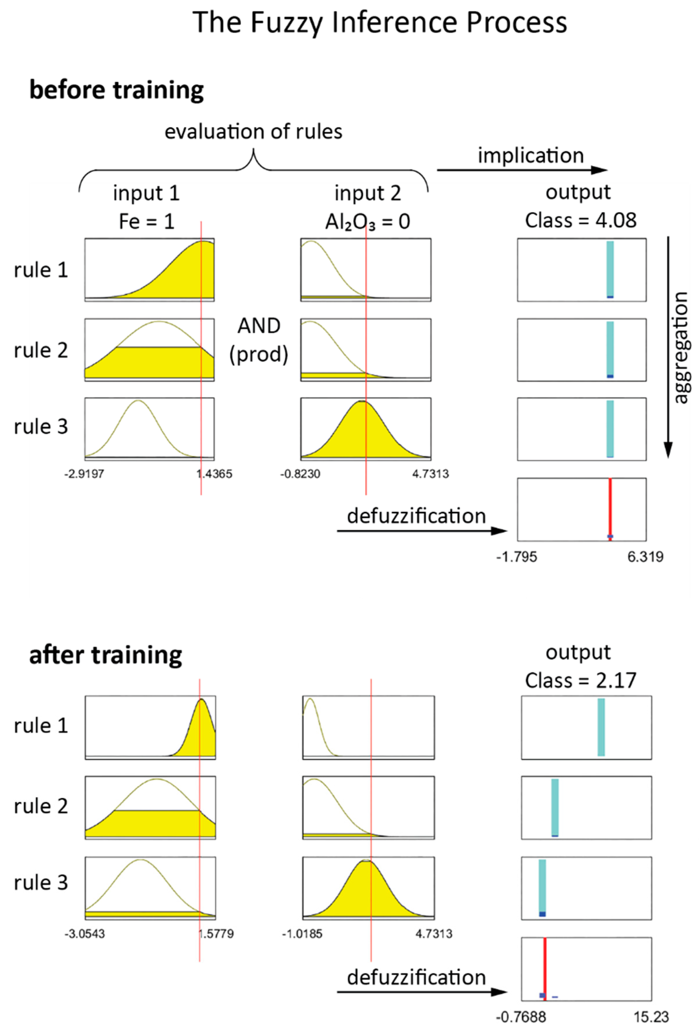
The fuzzy inference process, regarding the evaluation of rules and generating an output value, for the initial and the trained systems is illustrated in Figure 7. In addition to the parameters described above, the ‘minimum’ is used as the implication method to truncate the function from rule evaluation and the aggregated results are defuzzified using the weighted average method. The top plot in Figure 7 shows the process and the resulting class before training for an input of Fe% = 1 and Al₂O₃% = 0 (standardized values). The untrained system yields a class value of 4.08, which represents high-grade ore, but the high value for aluminum suggests a high shale content and the sample should be classified as class 2 or 2.5. The value of 2.17 for the trained system represents a value in the correct range.

3. Results

3.1. Data Set I

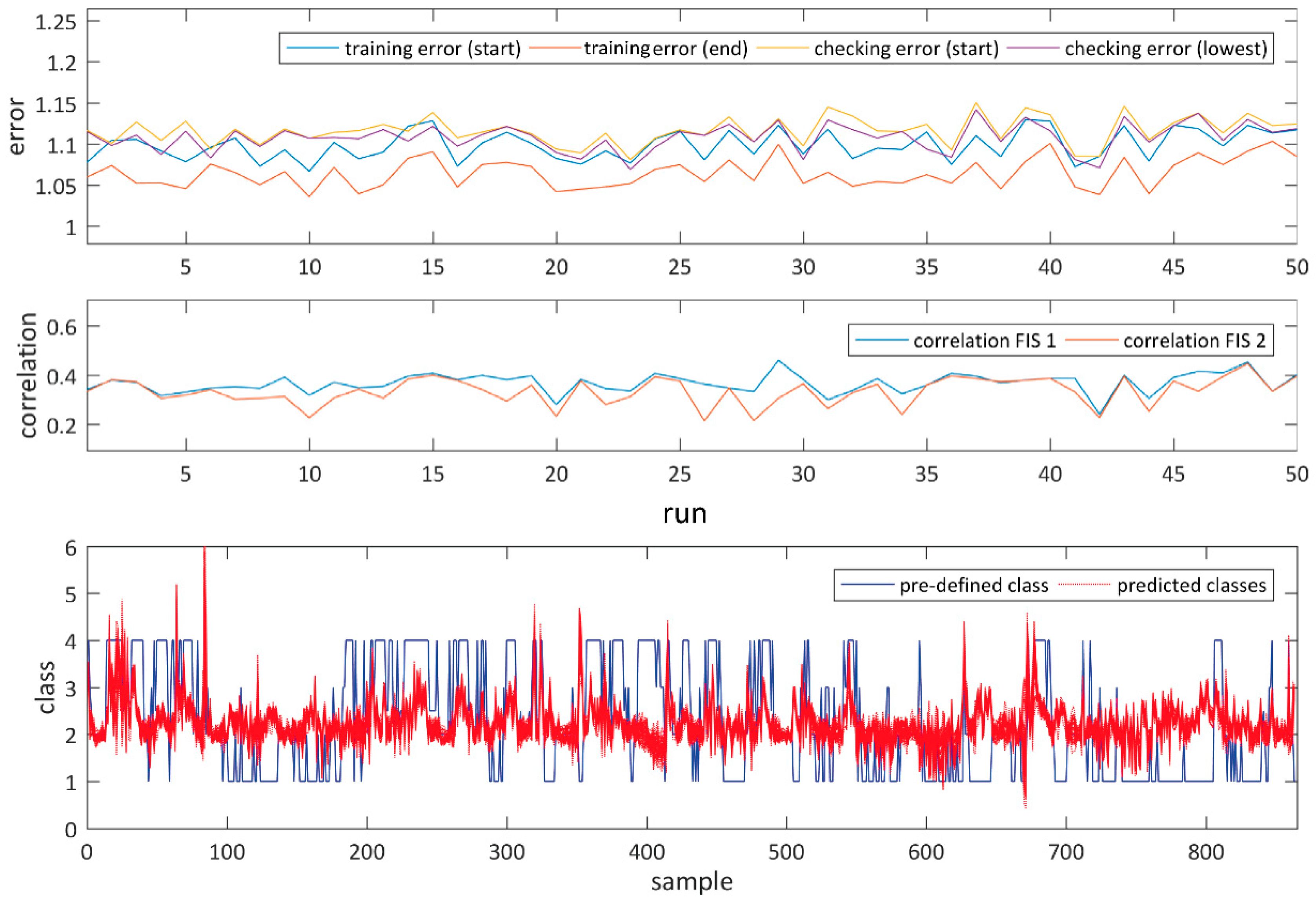
We applied the previously described fuzzy inference process to three different sets of input variables to evaluate which variables are best suited to predict iron ore lithology. From the total of 863 samples, 500 were chosen to design, train and check the inference system and the trained system tested on all 863 samples. The whole process, implemented in MATLAB, is run 50 consecutive times to evaluate its repeatability. We defined three clusters and a weighting exponent of m = 1.6 for this example. Random noise in the range of −0.2 and 0.2 was added/subtracted from the standardized data to generate the checking data, which should be similar but not identical to the training data and is important to avoid overfitting during training. Training and checking take place simultaneously and a training and checking error is recorded after each epoch (the algorithm was set to train for 100 epochs). Two trained fuzzy inference systems were saved and tested after this step, namely, the last one after 100 epochs (FIS 1) and the one with the lowest checking error (FIS 2). Only the FIS with the lowest checking error was used for subsequent prediction but both are compared in terms of performance (correlation of prediction to desired output class) in Figure 8 using Fe% and Al₂O₃% as the first set of input variables. The top plot shows the initial and final training errors as well as the initial and lowest checking errors for the 50 consecutive runs; the middle plot shows the correlation between the prediction from FIS 1 and the desired output, and FIS 2 and the desired output class. The correlation is well above 97% in most cases for both systems and the errors are very low. A comparison between predicted and pre-defined class in the bottom plot confirms the successful prediction based on iron and aluminum input variables.

We tested two additional input variable combinations, namely, Fe% and natural gamma as well as density and natural gamma, to evaluate if a substitution of petrophysical log data for assay data is feasible for lithology prediction. The results of predicting lithology from Fe% and natural gamma in Figure 9 indicate that a substitution of the gamma log for aluminum assay data is possible and successful with correlation above 94%.

The additional substitution of density for iron however gave poor results even after training. The match between predicted and pre-defined classes is below 1% (Figure 10, middle) and the errors are larger. We initially expected that density correlates well with iron content, but the distinct characteristics of the BIF host rocks and the mineralized iron ore formations result in Fe % showing a bimodal distribution while the density is normally distributed (Figure 11). BIF is a usually dense, non-porous rock composed of micro-crystalline silica (chert) and iron oxides (mainly magnetite). On the other hand, the mineralized, economically valuable iron ore formations are leached of their silica content and composed of predominantly hematite, which can be extremely friable. As a result, both rock types can have the same density whilst their iron grade is markedly different (~40% for the BIF and 60–70% for ore formations, densities ~3 g/cc, Figure 11). Although both iron oxide minerals have a similar density and magnetite is less abundant in the BIF compared to the concentrated hematite content in ore units, the different textural properties of the total rock mass result in similar density signatures. Consequently, distinguishing ore from BIF waste lithologies based on density and natural gamma is not possible in these cases.

To enable a near real-time classification of iron ore formations and grade estimation from petrophysical logs a different proxy for iron content is needed. As introduced previous, the spectral gamma-gamma ratio may be a better candidate to estimate iron content in iron bearing formations and we tested this hypothesis on SGG data from the second data set.

3.2. Data Set II

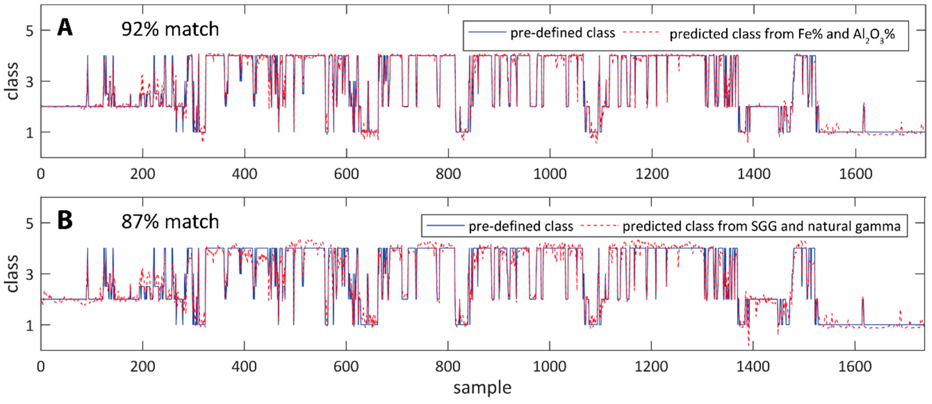
Some problems and difficulties with data preprocessing of the spectral data were introduced in previous sections to which the reader may refer for clarity. We used the Fe% and Al₂O₃% assay data to establish the predefined classes as before and tested two input variable combinations, namely (1) Fe% and Al₂O₃% and (2) SGG ratio and natural gamma. From the total of 1737 samples we selected 1000 for FIS training and applied the trained inference system to the total number of samples for prediction. We then selected the best-suited FIS based on the lowest checking error as before. Prediction results in Figure 12 show a match of 92% for the assay data and 87% for prediction from the SGG ratio and natural gamma log, indicating that iron grade can be successfully predicted from this data.

4. Conclusions

Firstly, our study highlights the benefits of using adaptive learning algorithms and inference systems to automate rock mass classification. In the case of using elemental assay data, this translates into efficient and objective classification as opposed to the current, slow process of manual input of classes into database systems, that is also prone to human error. For the case of using petrophysical data, gathered in near real-time, automated classification represents a necessary step to truly enable real-time interpretation and decision making.

Secondly, we show how petrophysics can substitute for, and circumvent the lengthy process of chemical analysis for iron ore grade estimation. Although the spectral gamma-gamma data used in our study is experimental in nature and not calibrated to a specific iron ore prospect, the lithology and grade prediction is over 80% correct. We expect the success rate to increase when the data is gathered from a distinct prospect with identical tool configuration and calibration. Therefore, spectral gamma-gamma logging in conjunction with fuzzy inference modeling for lithology prediction enables timely interpretation and classification of iron ore lithology and real-time decision making.

References

- Hillis, R.R.; Giles, D.; van der Wielen, S.E.; Baensch, A.; Cleverly, J.C.; Fabris, A.; Halley, S.W.; Harris, B.D.; Hill, S.M.; Kanck, P.A.; et al. Coiled tube drilling and real-time sensing—Enabling prospective drilling in the 21st century. Soc. Econ. Geol. 2014, 18, 243–259. [Google Scholar]
- Wanstedt, S. Geophysical logging applied to ore characterization in the Zinkgruvan mine, Sweden. Explor. Geophys. 1992, 23, 401–406. [Google Scholar] [CrossRef]
- King, A.; Fullagar, P.; Lamontagne, Y. Borehole geophysics in exploration, development, and production. In Proceedings of the Canadian Institute of Mining, Metallurgy Field Conference, Sudbury, ON, Canada, 4 September 1994. [Google Scholar]
- McDowell, G.; Fenlon, K.; King, A. SEG Technical Program Expanded Abstracts 2004; Society of Exploration Geophysicists: Tulsa, OK, USA, 2004; pp. 1151–1154. [Google Scholar]
- Conaway, J.; Killeen, P. Quantitative uranium determinations from gamma-ray logs by application of digital time series analysis. Geophysics 1978, 43, 1204–1221. [Google Scholar] [CrossRef]
- Virkkunen, R.; Hattula, A. Borehole Logging at LKAB Maalmberget Fe-Mine; Analys I Borrh l: Samnordiskt; Gruv Teknik: Ludvika, Sweden, 2000. [Google Scholar]
- McNally, G. The prediction of geotechnical rock properties from sonic and neutron logs. Explor. Geophys. 1990, 21, 65–71. [Google Scholar] [CrossRef]
- Elkington, P.; Stouthamer, P.; Brown, J. Rock strength predictions from wireline logs. Int. J. Rock Mech. Min. Sci. Geomech. Abstr. 1982, 19, 91–97. [Google Scholar] [CrossRef]
- Pechnig, R.; Haverkamp, S.; Wohlenberg, J.; Zimmermann, G.; Burkhardt, H. Integrated log interpretation in the German Continental Deep Drilling Program: Lithology, porosity, and fracture zones. J. Geophys. Res. Solid Earth 1997, 102, 18363–18390. [Google Scholar] [CrossRef] [Green Version]
- Maiti, S.; Krishna Tiwari, R.; Kümpel, H.-J. Neural network modelling and classification of lithofacies using well log data: A case study from KTB borehole site. Geophys. J. Int. 2007, 169, 733–746. [Google Scholar] [CrossRef]
- Ma, Y.Z.; Wang, H.; Sitchler, J.; Gurpinar, O.; Gomez, E.; Wang, Y. Mixture decompositions and lithofacies clustering from wireline logs. J. Appl. Geophys. 2014, 102, 10–20. [Google Scholar] [CrossRef]
- Urbancic, T.; Bailey, R. Statistical techniques applied to borehole geophysical data in gold exploration. Geophys. Prospect. 1988, 36, 752–771. [Google Scholar] [CrossRef]
- Fullagar, P.K.; Zhou, B.; Fallon, G.N. Automated interpretation of geophysical borehole logs for orebody delineation and grade estimation. Miner. Resour. Eng. 1999, 8, 269–284. [Google Scholar] [CrossRef]
- Templ, M.; Filzmoser, P.; Reimann, C. Cluster analysis applied to regional geochemical data: Problems and possibilities. Appl. Geochem. 2008, 23, 2198–2213. [Google Scholar] [CrossRef]
- Dekkers, M.J.; Heslop, D.; Herrero-Bervera, E.; Acton, G.; Krasa, D. Insights into magmatic processes and hydrothermal alteration of in-situ super-fast spreading ocean crust at ODP/IODP site 1256 from a cluster analysis of rock magnetic properties. Geochem. Geophys. Geosyst. 2014, 15, 3430–3447. [Google Scholar] [CrossRef]
- Imamura, S. SEG Technical Program Expanded Abstracts 1994; Society of Exploration Geophysicists: Tulsa, OK, USA, 1994; pp. 202–205. [Google Scholar]
- Trendall, A.F. The iron formations of the Hamersley Group, Western Australia, with special reference to the associated crocidolite. West. Aust. Geol. Surv. Bull. 1970, 119, 353. [Google Scholar]
- Killeen, P.; Mwenifumbo, C. Downhole Assaying in Canadian Mineral Deposits with the Spectral Gamma-Gamma Method; Report; International Atomic Energy Agency (IAEA): Vienna, Austria, 1988. [Google Scholar]
- Killeen, P.; Schock, L. Borehole assaying with the spectral gamma-gamma method: Some parameters affecting the SGG ratio. In Proceedings of the 4th International MGLS/KEGS Symposium on Borehole Geophysics for Minerals, Geotechnical and Groundwater Applications, Toronto, ON, Canada, 18–22 August 1991; pp. 399–406. [Google Scholar]
- Zadeh, L.A. Fuzzy sets. Inf. Control 1965, 8, 338–353. [Google Scholar] [CrossRef] [Green Version]
- Zadeh, L.A. Fuzzy logic. Computer 1988, 21, 83–93. [Google Scholar] [CrossRef]
- Bosch, D.; Ledo, J.; Queralt, P. Fuzzy logic determination of lithologies from well log data: Application to the KTB project data set (Germany). Surv. Geophys. 2013, 34, 413–439. [Google Scholar] [CrossRef]
- Ilkhchi, A.K.; Rezaee, M.; Moallemi, S.A. A fuzzy logic approach for estimation of permeability and rock type from conventional well log data: An example from the Kangan reservoir in the Iran Offshore Gas Field. J. Geophys. Eng. 2006, 3, 356–369. [Google Scholar] [CrossRef] [PubMed]
- Saggaf, M.; Nebrija, L. A fuzzy logic approach for the estimation of facies from wire-line logs. AAPG Bull. 2003, 87, 1223–1240. [Google Scholar] [CrossRef]
Figure 1.
Geological overview of the Pilbara region in Western Australia. The economically valuable banded-iron formations are hosted mainly by the Hamersley Group of the Mount Bruce Supergroup (after [17]).
Figure 2.
Stratigraphy of the Hamersley Group illustrating the position of the important iron formations in relation to major uneconomic shale, carbonate or volcanic units. Shale interbeds, illustrated for the Dales Gorge member to the right, internally subdivide the iron formations. The 17 BIF macrobands (grey) are separated by the 16 shale bands (black) that are used for stratigraphic correlation (after [17]).
Figure 3.
Sketch of the characteristics of a gamma ray spectrum recorded using a lithodensity tool with a 137Cs source. The high energy region of Compton scattering is indicative of the formation density, the gamma counts recorded in the low energy region are influenced by photoelectric absorption and indicative of density and average atomic number (Z) of a formation.
Figure 4.
Scatter plots of SGG ratio versus Fe%. Top plot shows the trend of the SGG ratio for the four different drillholes. The bottom plot shows the same data after shifting using drillhole (DH1) as a reference hole.
Figure 5.
Membership functions for the two input variables before training of the fuzzy inference system. The yellow functions define membership to cluster 1 (SHALE), the green to cluster 2 (BIF), the red to cluster 3 (ORE).
Figure 6.
Adjusted membership functions after training. The functions are spanning a considerably lower range than the initially defined functions in Figure 5 and thus reflect the desired output classes better.
Figure 7.
Illustration of the fuzzy inference process regarding the rule evaluation and output value generation. The three rules and three membership functions per input variable are the result of initial fuzzy c-means clustering. All rules are evaluated simultaneously and a logical operator and method (AND/PRODUCT in this case) as well as the implication method applied to the rule evaluation results. The aggregated fuzzy output set is finally defuzzified by choosing value of the weighted average. In this example, the input value is high in iron and high in aluminum and its membership in terms of iron is to cluster one and partly to cluster 2 but in terms of aluminum it is to cluster 3. The minimum (implication method) is chosen to truncate the output function (which is a linear function in this case). The truncated outputs are aggregated into a single fuzzy set of which the weighted average value is chosen as he crisp output (class) value.
Figure 8.
Results and parameters of the fuzzy inference system build from iron and aluminum input data. Top: training and checking errors for 50 consecutive runs; middle: correlation between prediction from the trained systems (FIS 1 is the last FIS from training (after 100 training epochs), FIS 2 is the system with the lowest checking error) and pre-defined classes indicating successful prediction (correlation above 97%); bottom: comparison of predicted and pre-defined classes from FIS 2.
Figure 9.
Results and parameters of the fuzzy inference system build from iron and natural gamma log input data. Training and checking error are low, as in the case of predicting from Fe% and Al2O3%; correlation between predicted and pre-defined classes is high as well (>94%) showing that a substitution of the natural gamma log for the aluminum assay is feasible for predicting iron ore lithologies.
Figure 10.
Results and parameters of the fuzzy inference system build from density and natural gamma log input data indicating that a substitution of density for iron content is not feasible for prediction of iron ore lithology.
Figure 11.
Heat scatter (data density) cross-plot of Fe% and density. There are two apparent groups of iron concentration, which both have similar densities. A prediction of iron grade based on density is therefore not possible.
Figure 12.
Comparison between predefined classes and predicted classes from elemental data (A) and petrophysical logs (B). Prediction based on elemental data shows an almost perfect match as would be expected, but prediction from SGG ratio and natural gamma shows a very good result as well.
© 2018 by the authors. Licensee MDPI, Basel, Switzerland. This article is an open access article distributed under the terms and conditions of the Creative Commons Attribution (CC BY) license (http://creativecommons.org/licenses/by/4.0/).
Share and Cite
MDPI and ACS Style
Kitzig, M.C.; Kepic, A.; Grant, A. Near Real-Time Classification of Iron Ore Lithology by Applying Fuzzy Inference Systems to Petrophysical Downhole Data. Minerals 2018, 8, 276. https://doi.org/10.3390/min8070276
AMA Style
Kitzig MC, Kepic A, Grant A. Near Real-Time Classification of Iron Ore Lithology by Applying Fuzzy Inference Systems to Petrophysical Downhole Data. Minerals. 2018; 8(7):276. https://doi.org/10.3390/min8070276
Chicago/Turabian StyleKitzig, Maria C., Anton Kepic, and Ashley Grant. 2018. "Near Real-Time Classification of Iron Ore Lithology by Applying Fuzzy Inference Systems to Petrophysical Downhole Data" Minerals 8, no. 7: 276. https://doi.org/10.3390/min8070276
Note that from the first issue of 2016, this journal uses article numbers instead of page numbers. See further details here.