What the Diffuse Layer (DL) Reveals in Non-Linear SFG Spectroscopy

Abstract

Following our recent work [Phys. Chem. Chem. Phys. 20:5190–99 (2018)] that provided the means to unambigously define and extract the three water regions at any charged interface (solid–liquid and air–liquid alike), denoted the BIL (Binding Interfacial Layer), DL (Diffuse Layer) and Bulk, and how to calculate their associated non-linear Sum Frequency Generation Spectroscopy (SFG) ${\chi }^2\left(\omega \right)$ spectroscopic contributions from Density Functional Theory (DFT)-based ab initio molecular dynamics simulations (DFT-MD/AIMD), we show here that the ${\chi }_{DL}^2\left(\omega \right)$ signal arising from the DL water region carries a wealth of essential information on the microscopic and macroscopic properties of interfaces. We show that the ${\chi }_{DL}^2\left(\omega \right)$ signal carries information on the surface potential and surface charge, the isoelectric point, EDL (Electric Double Layer) formation, and the relationship between a nominal electrolyte solution pH and surface hydroxylation state. This work is based on DFT-MD/AIMD simulations on a (0001) $\alpha$–quartz–water interface and on the air–water interface, with various surface quartz hydroxylation states and various electrolyte concentrations. The conclusions drawn make use of the interplay between experiments and simulations. Most of the properties listed above can now be extracted from experimental ${\chi }_{DL}^2\left(\omega \right)$ alone with the protocols given in this work, or by making use of the interplay between experiments and simulations, as described in this work.

1. Introduction

Non-linear vibrational Sum Frequency Generation Spectroscopy (SFG) probes non-centrosymmetric media, such that one tunable Infrared (IR) beam and one fixed visible beam are mixed at the interface between two media, and the recorded SFG intensity is due to the second-order susceptibility ${\chi }^{\left(2\right)}\left(\omega \right)$ of the interface. Since ${\chi }^{\left(2\right)}\left(\omega \right)$ is zero in media with inversion symmetry, like the bulk of liquids and many solids, the SFG signal will only arise from the molecules at the interface between the two media where the centrosymmetry is broken. The surface-specificity of SFG makes this technique a perfect tool to probe the microscopic arrangement of molecules in the interfacial layers, and for this reason, it has been widely used to unravel the water structure at aqueous interfaces. There is no need to stress the relevance of aqueous interfaces in many fields, from the key role played by water–air interfaces in atmospheric chemistry [1,2,3,4], through the effect of the interfacial water structure on protein folding and peptide bond formation [5,6,7], to the importance of silica–water interfaces in pollutant transport in underground water in mineral dissolution but also for drug delivery in our bodies [8,9]. The unique molecular arrangement at aqueous interfaces is at the basis of all the cited phenomena and its characterization is henceforth pivotal.

In our recent works [10,11], we especially showed how the first water monolayer is characterized by specific H-Bond networks that differ from the one known in bulk liquid water. Generally speaking, the interfacial network is built to either maximize water–water H-Bonds within the very first interfacial layer (as it is the case for hydrophobic interfaces like the air–water interface [10,12,13]) or to maximize interactions between water and a solid surface (as it is the case for hydrophilic surfaces like quartz–water [14]).

Although, on the one hand, non-linear SFG spectroscopy seems to be the perfect tool to reveal microscopic water arrangement at interfaces, it is, however, non-trivial to extract this information from SFG signals, especially because the interfacial thickness is unknown. Furthermore, recent works [15,16,17,18,19,20] have shown that the thickness probed in SFG experiments is probably the first water monolayer only for neutral interfaces (i.e., at the isoelectric point), while the field generated by charged surfaces reorients and polarizes water molecules in a thickness that is roughly estimated by the Debye length. The loss of inversion symmetry in the reoriented water slab thus increases the thickness probed in SFG experiments, presumably up to microns in the case of low ionic strengths. Unraveling the microscopic arrangement over large thicknesses seems thus rather complicated from SFG signals alone. However, in their seminal work , Tian et al. [15] showed that any charge interface is composed of only two distinct interfacial regions that are SFG active: the Binding Interfacial Layer (BIL), corresponding to the first water layer(s) at the interface, and the Diffuse Layer (DL), corresponding to the subsequent bulk water layer(s) reoriented by the surface field, which are SFG active because of the water reorientation along the surface field that breaks the liquid centrosymmetry. Beyond these two layers, centrosymmetric bulk liquid water is recovered. The additivity of the SFG signals in these two interfacial regions leads to

$${\chi }^{\left(2\right)}\left(\omega \right)={\chi }_{BIL}^{\left(2\right)}\left(\omega \right)+{\chi }_{DL}^{\left(2\right)}\left(\omega \right),$$

(1)

where only the BIL contribution to SFG is a “pure” ${\chi }^{\left(2\right)}\left(\omega \right)$ contribution, as it arises from a water structure that differs from bulk water, where inversion symmetry is broken due to the anisotropic nature of the interface. The DL region, however, would be centrosymmetric bulk water if the static field generated by the surface charge were not present. The SFG activity of this layer is thus the response of bulk water to three fields: the visible and IR beams used in the SFG experiment to which the static electric field generated at the charged surface is added. The ${\chi }^{\left(2\right)}\left(\omega \right)$ SFG signal arising from the DL can thus be expressed in terms of the non-linear third-order contribution ${\chi }_{bulk}^{\left(3\right)}\left(\omega \right)$ from bulk liquid water [11,15]:

$${\chi }_{DL}^{\left(2\right)}\left(\omega \right)={\chi }_{bulk}^{\left(3\right)}\left(\omega \right){\int }_{z_{BIL/DL}}^{z_{DL/Bulk}}dz·{\mathit{E}}_{DC}\left(z\right)e^{i\Delta k_{z}z},$$

(2)

where $\Delta {\varphi }_{DL}={\int }_{z_{BIL/DL}}^{z_{DL/Bulk}}dz·{\mathit{E}}_{DC}\left(z\right)$ is the electrostatic potential difference across the DL, with the DL being defined in between the two vertical boundaries denoted by $z_{BIL/DL}$ and $z_{DL/Bulk}$. In this expression, $\Delta k_z$ is a phase factor that takes into account interferences between the emitted light at different depths from the surface [15,16]. As shown by Roke et al. [16], interferences become relevant at low ionic strengths (i.e., below 10${}^{-2}$ M), where the Debye length is larger than 10 nm, therefore inducing a non-negligible phase mismatch between emitted SFG lights from different depths within the DL [16]. Light interferences can thus modulate the shape of the measured signal as demonstrated by Roke et al. [16] and Geiger et al. [17,18].

In our recent work [11], we developed a theoretical methodology to extract the BIL and DL water layers at any charged (or non-charged) interface, and their associated SFG signals fully ab-initio from Molecular Dynamics (MD) simulations.Our work uses Density Functional Theory (DFT)-based MD simulations, but the same strategy for defining BIL and DL layers works for any representation applied in the MD simulations (see, for instance, our recent work at the air–water interface based on classical force field MD [12,13]). Our theoretical approach is based on the recognition of water layers and their assignment into BIL/DL/Bulk regions. The layer identification and classification is based on the evaluation of three descriptors for water structural properties, namely the water density (which reveals water layers of various thicknesses), the water (average) coordination, and combined H-Bond strengths and orientations, that are applied to the unraveled layers. As shown in ref. [11], these descriptors provide an univocal definition of BIL/DL/Bulk layers in terms of water structural properties only; the electrolytes contained at interfaces are not directly included into the descriptors (but are, of course, indirectly taken into account into the descriptors). An identified water layer is assigned to the BIL if all above-mentioned structural descriptors differ from what is known in bulk liquid water. A layer is assigned to the DL region if all descriptors are identical to the ones in bulk liquid water, except for the reorientation of the H-Bond network. A layer is obviously assigned to the Bulk region if all descriptors are identical to the ones of bulk liquid water. We refer the reader to ref. [11] where our strategy was detailed, demonstrated and validated (and where comments have been written in order to avoid confusion between the here defined DL and the electrochemical diffuse layer).

Once the water layers have been defined, the deconvolution of BIL/DL contributions to SFG can be straightforwardly obtained by calculating the signal arising from the water molecules that belong to the BIL or to the DL. Moreover, once ${\chi }_{DL}^{\left(2\right)}\left(\omega \right)$ has been obtained, the third-order ${\chi }_{bulk}^{\left(3\right)}\left(\omega \right)$ spectrum can be unravelled by ${\chi }_{bulk}^{\left(3\right)}\left(\omega \right)={\chi }_{DL}^{\left(2\right)}\left(\omega \right)/\Delta {\varphi }_{DL}$. Comparing the ${\chi }_{bulk}^{\left(3\right)}\left(\omega \right)$ spectra hence calculated for various aqueous interfaces, we demonstrated in ref. [11] that ${\chi }_{bulk}^{\left(3\right)}\left(\omega \right)$ is indeed the ${\chi }_{bulk}^{\left(3\right)}\left(\omega \right)$ of bulk liquid water—hence, a universal signal.

In ref. [11], the decomposition of the total SFG signal into BIL and DL contributions was used to isolate the ${\chi }_{BIL}^{\left(2\right)}\left(\omega \right)$ signal, hence recovering the BIL-specificity of the SFG signal, i.e., the interfacial signal related to the water in direct contact with the surface. In the present work, we move the focus to the DL-SFG contribution, showing how the ${\chi }_{DL}^{\left(2\right)}\left(\omega \right)$ signal not only provides a direct and quantitative measure of the $\Delta {\varphi }_{DL}$ electrostatic potential across the DL, and thus, the net surface charge (in the BIL, i.e., at the interface), but we also show that this signal is directly sensitive to the ion distribution at interfaces, thus providing a means to discriminate if an Electric Double Layer (EDL) is formed at a given charged interface. The identification and characterization of EDLs is of pivotal importance for interfacial chemical reactivity, which is highly relevant, for instance, for reactions taking place at electrode/electrolyte interfaces in electrochemistry. Moreover, we provide proof of concept that the ${\chi }_{DL}^{\left(2\right)}\left(\omega \right)$ signal can be used to measure the interfacial ionic concentration (in the BIL) and/or the degree of hydroxylation of a solid surface in contact with water.

2. Computational Methods

Density Functional Theory-based Molecular Dynamics (DFT-MD) simulations are performed on (0001) $\alpha$-quartz–liquid water (QW) and air–liquid water (AW) interfaces varying the protonation state of the oxide surface (from fully hydroxylated to 12% deprotonation of the surface hydroxyls) and varying electrolyte concentrations (varying the number of aqueous KCl ion pairs, QW and AW). Various ionic arrangements have been obtained along the trajectories, resulting in different net ionic concentrations within the interfacial layer, i.e., within the BIL. All statistically relevant configurations explored during the simulations (with relative time of sampling) are reported in

Table 1. Details of the simulations performed in this work. QW stands for the $\alpha$-(0001) quartz–water interface and AW for the air–water interface. “% dep” means % deprotonation of the quartz surface hydroxyls. BIL is the Binding Interfacial Layer.

System	Time Length (ps)	Box (Å${}^3$)	% Dep	#H(D)${}_2$O in the Box	#KCl in the Box	Ion Species in the BIL	[ion]${}_{\mathit{BIL}}$(M)
QW-1	20.0	9.82 × 8.50 × 32.16	0	64	0	/	0.0
QW-2	20.0	15.64 × 17.01 × 52.16	0	512	1	K${}^{+}$	1.6
QW-3	18.4	15.64 × 17.01 × 52.16	0	512	4	K${}^{+}$	4.2
QW-4	20.0	9.82 × 8.50 × 32.16	0	64	1	K${}^{+}$	7.1
QW-5	20.0	9.82 × 8.50 × 32.16	3	64	0	/	0.0
QW-6	20.0	15.64 × 17.01 × 52.16	3	512	1	/	0.0
QW-7	20.0	15.64 × 17.01 × 52.16	3	512	1	K${}^{+}$	1.6
QW-8	20.0	9.82 × 8.50 × 32.16	12	64	0	/	0.0
QW-9	13.6	9.82 × 8.50 × 32.16	12	64	1	K${}^{+}$	5.2
QW-10	15.1	9.82 × 8.50 × 32.16	12	64	1	K${}^{+}$	7.1
AW-1	20.0	19.73 × 19.73 × 35.00	0	256	1	/	0.0
AW-2	20.0	19.73 × 19.73 × 35.00	0	256	1	Cl${}^{-}$	1.0

.

All DFT-MD simulations presented in Table 1 were performed with the CP2K package [21,22]. The BLYP [23,24] functional was adopted in combination with mixed Gaussian–Plane Waves basis sets and Goedecker-Tetter-Hutter (GTH) pseudopotentials [25]. Grimme D2 corrections [26,27] are taken into account for a better description of van der Waals interactions. Default algorithms and convergence criteria were adopted. Box-sizes (see Table 1) were chosen in order to reproduce the density of bulk water and periodic boundary conditions were applied in all three spatial directions. Born–Oppenheimer dynamics were performed, the electronic wavefunction was calculated at each time step, the classical nuclei displacements were obtained through the Velocity–Verlet algorithm, and the time-step was 0.4 fs. As can be seen in Table 1, some simulation boxes were charge neutral (electrolytes are introduced as ion-pairs), and others were charged because of surface silanol deprotonations. For these later ones, a uniform background and the Ewald summation for electrostatics take care of the total charge in the interactions. This is standard procedure in DFT-MD simulations.

The electronic set-up followed our previous works [10,28,29] on similar interfaces, adequately providing the structural and vibrational properties of these interfaces. In the case of water(D${}_2$O)–air interfaces (simulations AW-1 and AW-2 in Table 1), the DZVP-MOLOPT-SR basis set, augmented with a 400 Ry plane wave basis set was used. In the case of the quartz–water(H${}_2$O) interfaces, a plane wave basis-set cutoff of 280 Ry combined with a TZV2P Gaussian basis set for O, Si, Cl, and H atoms, and the DZVP-MOLOPT-SR was used for K and I atoms.

DFT-MD simulations are systematically divided into two parts, an equilibration dynamics of 5 ps duration (in the microcanonical NVE ensemble, however, allowing rescaling of velocities whenever necessary,) followed by pure NVE production runs (see Table 1 for the associated time lengths over which structural and spectroscopic properties are calculated). For structural and spectroscopic analyses, the vector normal to the surface is taken oriented towards the vacuum (AW) or towards the solid (QW).

The identification of the water interfacial layers at charged (and non-charged) interfaces, namely the BIL (Binding Interfacial Layer), DL (Diffuse Layer) and Bulk liquid water, was obtained by following our methodology that was derived and fully described in ref. [11] on the basis of water structural properties only. In the systems investigated here, the BIL was found to be systematically composed of the first water monolayer.

The non-linear SFG (Sum Frequency Generation) signal arises from both BIL amd DL layers only, while the centrosymmetric bulk water layer is not SFG-active (this is verified in our calculations). The total resonant electric dipole non-linear susceptibility, ${\chi }^{\left(2\right)}\left(\omega \right)$, and its real and imaginary components were calculated following the time-dependent method of Morita and Hynes [30,31], using the model proposed by Khatib et al. [32] for dipole and polarisability derivatives. As shown in our previous works, this model gives accurate SFG spectra [10,11]. Briefly, supposing that in the high frequency region (>3000 cm${}^{-1}$) , only the O–H stretching motions contribute to the spectrum and neglecting intermolecular cross-correlation terms, one has

$$\begin{array}{c}\hfill {\chi }_{PQR}^{\left(2\right)}\left(\omega \right)=\sum _{m=1}^M\sum _{n_1=1}^2\sum _{n_2=1}^2\frac{i}{k_{b}T\omega }\times {\int }_0^{\infty }dt{e}^{(-i\omega t)}\langle {\dot{\alpha }}_{PQ}^{m,n_1}\left(t\right){\dot{\mu }}_R^{m,n_2}\left(0\right)\rangle ,\end{array}$$

(3)

where (P,Q,R) are any $x,y,z$ directions in the laboratory frame, and k${}_b$ and T are the Boltzmann constant and temperature of the simulated system, respectively. $\langle \cdots \rangle$ is a time-correlation function; ${\alpha }_{PQ}\left(t\right)$ and ${\mu }_R\left(0\right)$ are, respectively, the individual O–H bond contribution to the total polarization and dipole moment of the system; and ${\dot{\alpha }}_{PQ}\left(t\right)$ and ${\dot{\mu }}_R\left(0\right)$ are their time derivatives. M is the number of water molecules, and $n_1$ and $n_2$ are two indexes that identify each of the two O–H oscillators per molecule. We here calculate $ssp$ SFG signals, i.e., $xxz$ directions. Note that the electric-dipole approximation was used here, and electric-quadrupole contributions to the $ssp$ signal were neglected. Using the direction cosine matrix (D) projecting the molecular frame $(x,y,z)$ onto the laboratory frame $(P,Q,R)$, and assuming that the O–H stretching is much faster than the modes involving a bond reorientation, one can write

$$\begin{array}{ccc}\hfill {\dot{\alpha }}_{PQ}\left(t\right)& \simeq & \sum _i^{x,y,z}\sum _j^{x,y,z}{D}_{Pi}\left(t\right)D_{Qj}\left(t\right)\frac{d{\alpha }_{ij}}{d{r}_z}{v}_z\left(t\right)\hfill \end{array}$$

(4)

$$\begin{array}{ccc}\hfill \dot{{\mu }_R}\left(t\right)& \simeq & \sum _i^{x,y,z}{D}_{Ri}\left(t\right)\frac{d{\mu }_i}{d{r}_z}{v}_z\left(t\right).\hfill \end{array}$$

(5)

The D matrix and the projection of the velocities on the O–H bond axis ($v_z$) can be readily obtained from the DFT-MD trajectory, while $\frac{d{\alpha }_{ij}}{d{r}_z}$$\frac{d{\mu }_i}{d{r}_z}$ are parametrized [32,33].

SFG spectra arising from the BIL (respectively, from the DL and the Bulk) were obtained, including only the water molecules that belong to BIL/DL/Bulk into the summation in Equation (3), as unraveled from our decomposition scheme [11] for recoginizing these layers.

Electric fields, (${\mathit{E}}_{DC}\left(z\right)$), and differences in electric potentials ($\Delta \varphi$) were obtained fully ab-initio from the optimized electronic wavefunction, and the positions of the nuclei, using the standard routine implemented in CP2K. ${\mathit{E}}_{DC}\left(z\right)$ were calculated each 100 fs during the dynamics and then averaged over all sampled data.

3. Results and Discussion

3.1. ${\chi }_{DL}^{\left(2\right)}\left(\omega \right)$: A Unique Shape but Various Signs and Magnitudes—A Direct Measure of the Surface Potential and of the Isoelectric Point

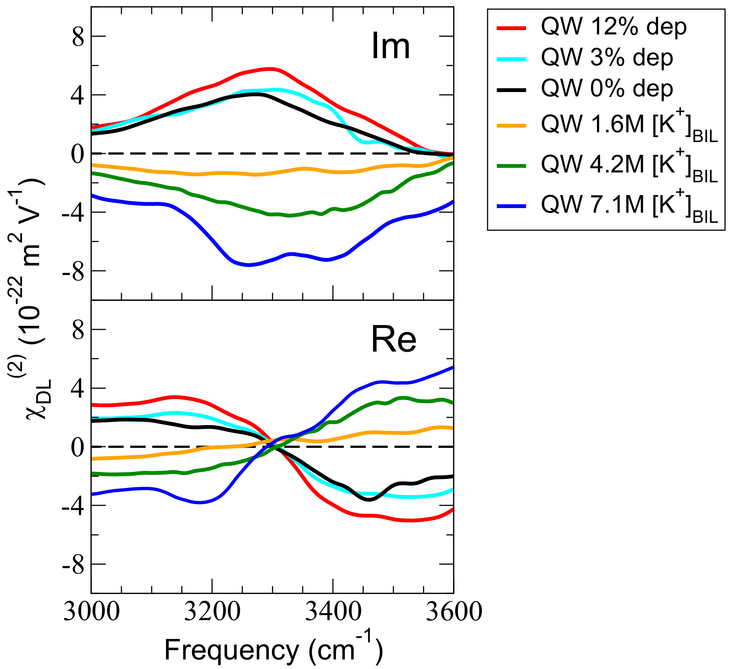
Figure 1 reports the SFG ${\chi }_{DL}^{\left(2\right)}\left(\omega \right)$ spectra (Imaginary Im${\chi }^{\left(2\right)}\left(\omega \right)$ and Real Re${\chi }^{\left(2\right)}\left(\omega \right)$ components of ${\chi }_{DL}^{\left(2\right)}\left(\omega \right)$), calculated from state-of-the-art Density Functional Theory-based Molecular Dynamics simulations (DFT-MD) on (0001) $\alpha$-quartz–liquid water (QW) interfaces, where the degree of hydroxylation of the surface is varied or with various concentrations of aqueous KCl electrolyte. The model and structural properties for the neat aqueous (0001) $\alpha$-quartz–liquid water (QW) interface were presented in our earlier works [14,28] and all details for the simulation set-ups are presented in the computational section and in Table 1. The fully hydroxylated aqueous surface (0% deprotonation in the present nomenclature) represents PZC conditions (Point of Zero Charge, pH∼2–4), in agreement with literature [34]. The systems presented in Figure 1 have a deprotonation state of 0% (this is the neat QW interface, fully hydroxylated), 3% dehydroxylation (QW 3% dep) and 12% dehydroxylation (QW 12% dep) (all interfaces are free of electrolytes), or are composed of the neat QW interface accomodating varied concentrations of excess K${}^{+}$ cation located in the BIL (Binding Interfacial Layer), i.e., 1.6 M, 4.2 M and 7.1 M. In the simulations, the excess ionic concentrations were obtained by locating the cations in the BIL, while the anions were located farther away from the surface in the DL (Diffuse Layer). These cation/anion relative positions correspond to our previous findings [28,29]. We refer the readers to the methods section for details about the simulations and ${\chi }_{DL}^{\left(2\right)}$ calculations.

The BIL and DL layers were identified following the methodology developed in our group [11], as well as the deconvolution of BIL and DL contributions to the Im${\chi }_{DL}^{\left(2\right)}\left(\omega \right)$ spectrum (and the Re${\chi }_{DL}^{\left(2\right)}\left(\omega \right)$ spectrum, not discussed here, however). As shown and discussed in ref. [11], the shape of the Im${\chi }_{DL}^{\left(2\right)}\left(\omega \right)$ signal is given by Im${\chi }_{bulk}^{\left(3\right)}\left(\omega \right)$ (third-order, non-linear susceptibility of bulk water), while the sign and magnitude of Im${\chi }_{DL}^{\left(2\right)}\left(\omega \right)$ differ for the various interfaces because of the dependence on the $\Delta {\varphi }_{DL}$ (Hartree) electric potential across the DL through ${\chi }_{DL}^{\left(2\right)}\left(\omega \right)={\chi }_{bulk}^{\left(3\right)}\left(\omega \right)\Delta {\varphi }_{DL}$. ${\chi }_{DL}^{\left(2\right)}\left(\omega \right)$ is, therefore, a direct measure of the electric potential across the DL and hence, a direct measure of the surface potential/field.

At the neat QW interface (PZC, 0% deprotonation, black curve in Figure 1), there is a positive Im${\chi }_{DL}^{\left(2\right)}\left(\omega \right)$ signal; as already shown in our previous works [14,28], there is a net negative surface charge at the QW that originates from the structural motifs of alternate in-plane/out-of-plane orientations of the O–H silanol surface terminations and associated polarization/charge transfers with the H-bonded water molecules. This gives rise to the positive Im${\chi }_{DL}^{\left(2\right)}\left(\omega \right)$ signal (the normal to the surface is taken directed towards the solid as convention in SFG, see computational details). As expected, there is an increase in magnitude of the Im${\chi }_{DL}^{\left(2\right)}\left(\omega \right)$ response with increasing surface deprotonation (3% and 12% of surface silanols deprotonated, light blue and red lines in Figure 1). On the contrary, when there is KCl electrolyte, with the K${}^{+}$ cations adsorbed at the silica surface and the Cl${}^{-}$ anions located farther away from the surface (this is not imposed in the simulation, but it is the result of the preference of these ions at the quartz–water interface, see the full demonstration in refs. [28,29]), a net positive charge is now created in the BIL because of the presence of the cations in the BIL water layer. The Im${\chi }_{DL}^{\left(2\right)}\left(\omega \right)$ is consequently negative in sign, and its magnitude becomes more and more negative with the increase in [K${}^{+}$]${}_{BIL}$ (yellow, green, and blue curves in Figure 1).

One last comment is that because the ${\chi }_{bulk}^{\left(3\right)}\left(\omega \right)$ signal has two bands, respectively located at 3200 and 3400 cm${}^{-1}$ (see our calculations in ref. [11] and Tian et al.’s experimental demonstration [15]), the ${\chi }_{DL}^{\left(2\right)}\left(\omega \right)$ signal also systematically displays these two bands.

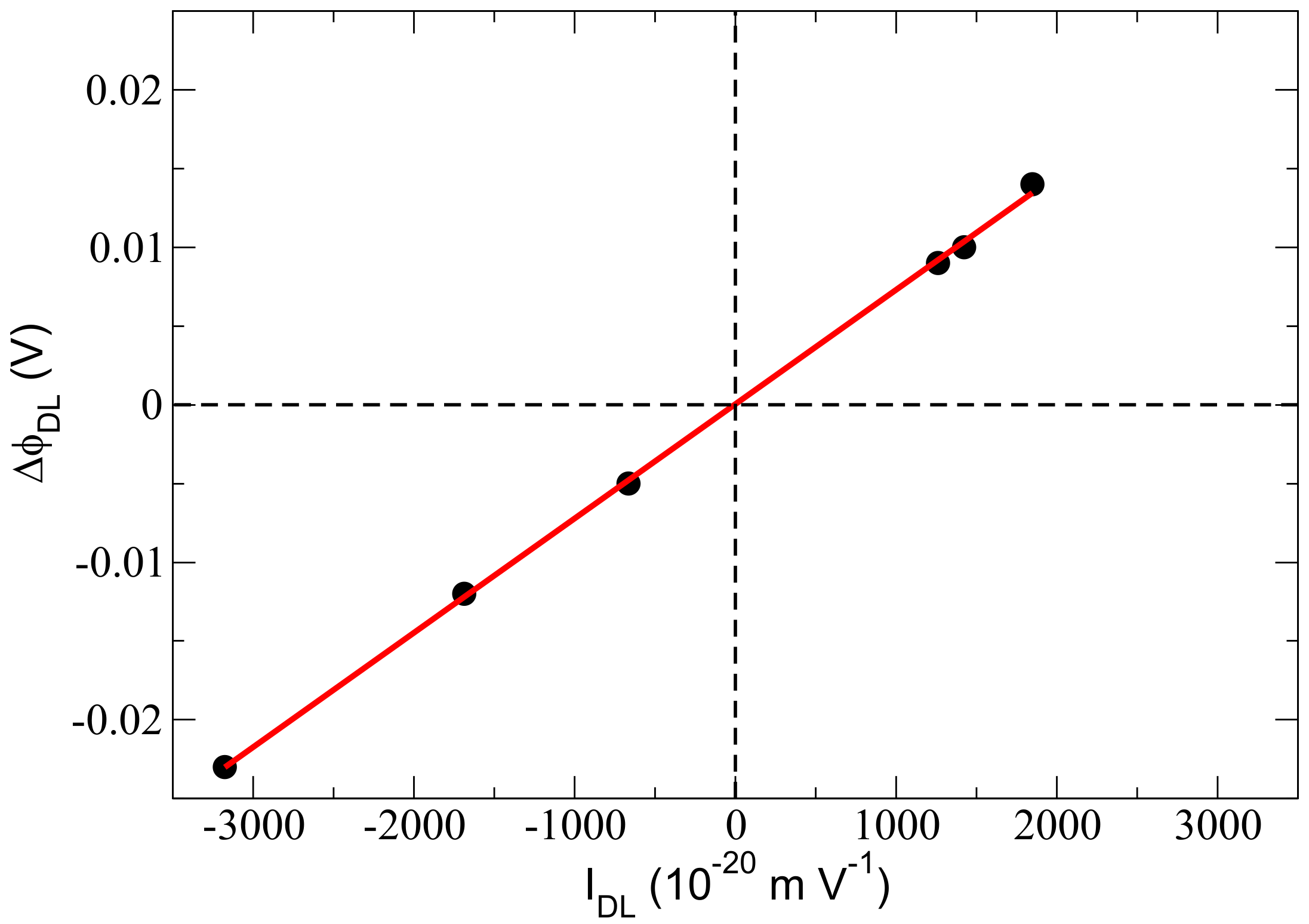
If we now compute the integral of Im${\chi }_{DL}^{\left(2\right)}\left(\omega \right)$ in the region between 3000 and 3600 cm${}^{-1}$, denoted $I_{DL}$ in the rest of the text, and plot it against $\Delta {\varphi }_{DL}$ (electric potential across the DL) calculated fully ab-initio from the DFT-MD simulations for all investigated interfaces presented in Figure 1, a straight line is obtained, as shown in Figure 2. This correlation obviously follows the equation

$$\Delta {\varphi }_{DL}=\frac{I_{DL}}{I_{{\chi }_{bulk}^{\left(3\right)}}},$$

(6)

where $I_{{\chi }_{bulk}^{\left(3\right)}}$ is the integral of Im${\chi }_{bulk}^{\left(3\right)}\left(\omega \right)$ from 3000 to 3600 cm${}^{-1}$. $I_{{\chi }_{bulk}^{\left(3\right)}}=1370\times {10}^{-18}$ m V${}^{-2}$ is calculated from the slope of the linear regression in Figure 2; it is $I_{{\chi }_{bulk}^{\left(3\right)}}=1374\times {10}^{-18}$ m V${}^{-2}$ from the integral of Im${\chi }_{bulk}^{\left(3\right)}\left(\omega \right)$ extracted from our previous DFT-MD trajectory of bulk liquid water subjected to a constant external field (imposed) (see ref. [11]). This latter value is identical (within 0.2% error) to the ones obtained from direct integration of the theoretical Im${\chi }_{bulk}^{\left(3\right)}\left(\omega \right)$ calculated for various quartz–water and air–water interfaces in our previous ref. [11] and calculated from Tian and Shen’s 2016 experimental measurement of Im${\chi }_{bulk}^{\left(3\right)}\left(\omega \right)$ [15].

Since ${\chi }_{bulk}^{\left(3\right)}\left(\omega \right)$ has the same signal at all aqueous interfaces [11,15], the value of $I_{{\chi }_{bulk}^{\left(3\right)}}$ calculated here provides the means to extract $\Delta {\varphi }_{DL}$, the electrostatic potential across the DL at any aqueous interface directly from the knowledge of Im${\chi }_{DL}^{\left(2\right)}\left(\omega \right)$ and $I_{DL}$ (Equation (6)). This can be done by both experimental and computational communities. We remind the reader that $\Delta {\varphi }_{DL}$ is not needed in order to extract Im${\chi }_{DL}^{\left(2\right)}\left(\omega \right)$ from the DFT-MD simulations, as it is obtained through Equation (3), taking into account only the water molecules that belong to the DL into the summation (over m). From simulations, Im${\chi }_{DL}^{\left(2\right)}\left(\omega \right)$ and $I_{DL}$ can thus be readily extracted, as shown above, and the use of Figure 2 leads to the associated value of $\Delta {\varphi }_{DL}$. The latter is, therefore, done without the computationally expensive step of calculating $\Delta {\varphi }_{DL}$ from the ab initio representation or without requiring a simplified model for the electrostatic potential (i.e., Gouy–Chapman, for instance). If one does SFG experiments, Im${\chi }_{DL}^{\left(2\right)}\left(\omega \right)$ can be extracted, for instance, following Tian et al.’s strategy [15] and correcting for the interference effects [16,17], and hence, $I_{DL}$ is known from the experiment, and a search in Figure 2 for $\Delta {\varphi }_{DL}$ can be readily done.

Furthermore, SFG spectroscopy can be used, by both the experimental and theoretical communities to directly measure the isoelectric point of any given aqueous interface, which simply corresponds to the conditions (pH, electrolytes concentration) for which $I_{DL}$=0 (see Figure 2). One more comment is that as $I_{DL}\mathrm{vs}{I}_{{\chi }_{bulk}^{\left(3\right)}}$ is a linear relationship, two points are enough to reveal the isoelectric point at which $I_{DL}$=0. This is, therefore, not a complicated matter in SFG experiments, as PZC conditions are (usually) systematically sampled, and one has to do one more experiment either at more basic or more acidic conditions to reveal the isoelectric point. The same comment applies for DFT-MD simulations—two simulations are enough to reveal the isoelectric point.

3.2. ${\chi }_{DL}^{\left(2\right)}\left(\omega \right)$ and EDL Formation

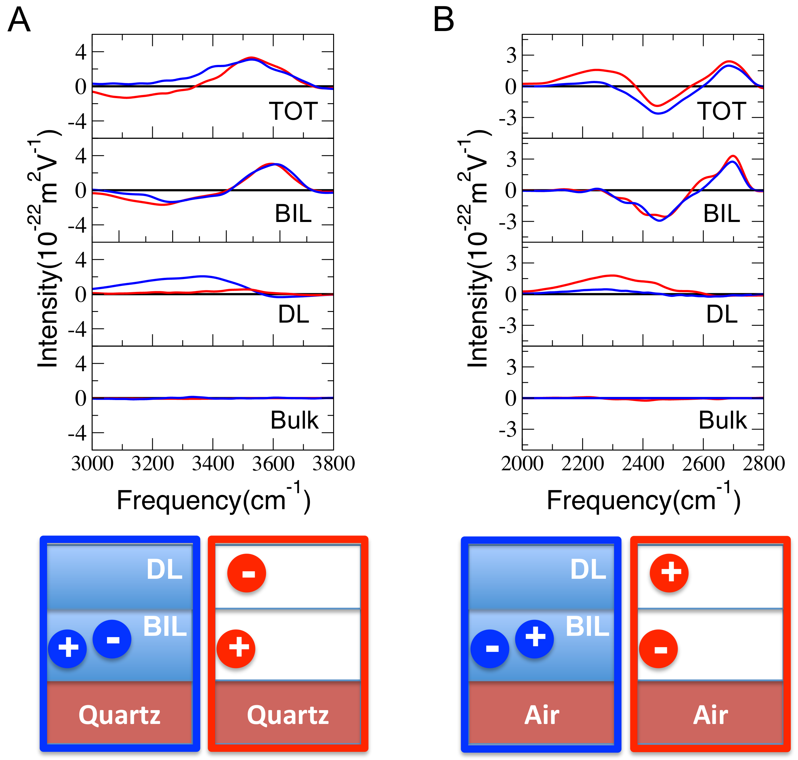
We now demonstrate that ${\chi }_{DL}^{\left(2\right)}\left(\omega \right)$ is sensitive to EDL (Electric Double Layer) formation, and we show how to characterize the EDL directly by means of SFG spectroscopy and by means of ${\chi }_{DL}^{\left(2\right)}\left(\omega \right)$ only. To that end, two test cases are presented: (1) the QW interface with 3% surface silanol deprotonation and one aqueous KCl ion pair (518 H${}_2$O molecules in the simulation box, see Table 1), and (2) the water–air interface (WA) at pH = 7 with one aqueous KCl ion pair (256 D${}_2$O molecules in the simulation box, see Table 1). Refer to the methods section for all computational details, and see schemes at the bottom of Figure 3 for illustrations. For the QW interface, two ionic configurations were imposed at the start of the simulation and maintained over the simulation time-scale of the DFT-MD trajectory (without imposing constraints): (a) the two ions of the KCl electrolyte were respectively located in the BIL (K${}^{+}$) and in the DL (Cl${}^{-}$) over the length of the simulation, and (b) the two ions of the KCl electrolyte were both simultaneously located in the BIL, forming a contact ion pair (CIP). Similarly, two ionic configurations were maintained over the length-scale of the DFT-MD simulation at the WA interface: (a) one ion per water layer, i.e., Cl${}^{-}$ in the BIL and K${}^{+}$ in the DL, and (b) the two ions of the KCl electrolyte were both simultaneously located in the BIL forming a contact ion pair (CIP). The relative locations of K${}^{+}$ in the BIL and Cl${}^{-}$ in the DL at the QW and the reverse at the AW are the result of our previous investigations (see refs. [11,28,29]. From the point of view of these structures, an electrolytic configuration where the excess of one ion species is located in the BIL corresponds to an EDL formation, while the electrolytic CIP configuration located in the BIL does not lead to the formation of an EDL.

Our structural and spectral decomposition schemes [11] were applied to the four above-mentioned systems and trajectories, so BIL/DL/Bulk SFG signatures have been deconvolved from the total Im${\chi }^{\left(2\right)}\left(\omega \right)$ signal. The total and deconvolved Im${\chi }^{\left(2\right)}\left(\omega \right)$ spectra are presented in Figure 3. The following discussions use only these signals, i.e., Im${\chi }_{BIL}^{\left(2\right)}\left(\omega \right)$, Im${\chi }_{DL}^{\left(2\right)}\left(\omega \right)$, and Im${\chi }_{bulk}^{\left(2\right)}\left(\omega \right)$ (equal to zero, as can be seen in Figure 3) to assess how water is organised in the BIL and DL interfacial layers and to reveal the EDL formation directly from the Im${\chi }_{DL}^{\left(2\right)}\left(\omega \right)$ signal.

Starting with the QW interface, our deconvolution (Figure 3A) clearly shows that the water structure in the BIL of the “QW 3% dep” interface, perturbed by the presence of K${}^{+}$ [11,28,29] is not furthermore disordered when also the Cl${}^{-}$ is located in the BIL (no-EDL); the blue and red Im${\chi }_{BIL}^{\left(2\right)}\left(\omega \right)$ signals are indeed equal for the two ionic configurations (EDL/red and no-EDL/blue). Refer to our previous works [14,28,29] for full characterization of the BIL structure in response to the presence of the ions. While the Im${\chi }_{BIL}^{\left(2\right)}\left(\omega \right)$ signal is, hence, not able to provide a distinct signal between the two electrolyte configurations (EDL vs. no-EDL), Im${\chi }_{DL}^{\left(2\right)}\left(\omega \right)$ however, shows changes in the SFG spectroscopy of this layer, depending on whether an EDL or a no-EDL situation exists; a positive Im${\chi }_{DL}^{\left(2\right)}\left(\omega \right)$ was indeed predicted when no-EDL was formed (K${}^{+}$–Cl${}^{-}$ CIP contact ion pair in the BIL, blue signal in Figure 3A) while virtually no signal was obtained from the DL when there was excess [K${}^{+}$]${}_{BIL}$ cations located in the BIL and an EDL is formed. When only the K${}^{+}$ ions are located in the BIL (one K${}^{+}$ in the present simulation box), the cations accumulate at the interface in order to screen the surface charge (negative quartz surface charge at the interface with water [29] for the fully hydroxylated surface, made even more negative here by dehydroxylation of the surface). The positive charge carried by the cation hence compensates the negative charge of the deprotonated quartz surface, leading to a net negligible charge in the BIL (i.e., at the interface) and thus, the absence of spectroscopic SFG activity from the DL (no surface field inducing the formation of the reoriented DL). When the Cl${}^{-}$ anion is closer to the silica surface, located in the BIL together with the K${}^{+}$ cation, the net charge in the BIL is again negative (thus giving rise to a very similar situation to the one without electrolytes, i.e., neat QW interface), and a positive Im${\chi }_{DL}^{\left(2\right)}\left(\omega \right)$ is hence measured.

The DL sensitivity to the respective positions of the cations/anions is confirmed at the AW interface, see Figure 3B. This latter interface is neutral by construction, which makes the discussion easier once electrolytes are adsorbed at the interface. The Im${\chi }_{BIL}^{\left(2\right)}\left(\omega \right)$ signal is, again, unable to provide data that would allow the EDL and no-EDL electrolytic configurations to be distinguished, as these two structural arrangements have the same SFG-BIL spectra (blue and red lines in Figure 3B), while the SFG-DL spectra are different for these two configurations. Im${\chi }_{DL}^{\left(2\right)}\left(\omega \right)$ is non-zero for the configuration where the Cl${}^{-}$ anion is located in the BIL and the K${}^{+}$ cation is in the DL, giving rise to an EDL (red line in Figure 3B). Because the neat AW interface is neutral, the net charge in the BIL is negative once there is an excess Cl${}^{-}$ concentration in the BIL [Cl${}^{-}$]${}_{BIL}$, leading to a positive Im${\chi }_{DL}^{\left(2\right)}\left(\omega \right)$ (red line in Figure 3B), while the charge in the BIL becomes zero when both Cl${}^{-}$ and K${}^{+}$ are located in the BIL (no-EDL); thus, there is no surface field and no DL formation (and a zero DL-SFG signal).

As demonstrated by these test cases, the Im${\chi }_{DL}^{\left(2\right)}\left(\omega \right)$ spectroscopic SFG signal provides direct knowledge of the EDL formation at any electrolytic aqueous interface. This requires knowledge of the Im${\chi }_{DL}^{\left(2\right)}\left(\omega \right)$ signal at the neat interface, which is taken as the reference for the following conclusions:

• If the ions of the electrolyte do not form an EDL, there is no change in the Im${\chi }_{DL}^{\left(2\right)}\left(\omega \right)$ intensity of the electrolytic interface when compared to the Im${\chi }_{DL}^{\left(2\right)}\left(\omega \right)$ of the neat reference interface.
• If an EDL is formed by the electrolytes and the cations are preferentially adsorbed in the BIL, there is a decrease in the Im${\chi }_{DL}^{\left(2\right)}\left(\omega \right)$ intensity with respect to the Im${\chi }_{DL}^{\left(2\right)}\left(\omega \right)$ of the neat reference interface.
• If an EDL is formed by the electrolytes and the anions are preferentially adsorbed in the BIL, there is an increase in the Im${\chi }_{DL}^{\left(2\right)}\left(\omega \right)$ intensity with respect to the Im${\chi }_{DL}^{\left(2\right)}\left(\omega \right)$ of the neat reference interface.

This provides the protocol that experimentalists can apply to their Im${\chi }_{DL}^{\left(2\right)}\left(\omega \right)$ signals to compare the neat interface signal and the signal at the electrolytic interface, without the need to systematically resort to computational simulations.

Now that the ability of the SFG spectroscopy (within the framework of our deconvolution scheme for BIL & DL water layers and associated Im${\chi }_{BIL}^{\left(2\right)}\left(\omega \right)$ & Im${\chi }_{DL}^{\left(2\right)}\left(\omega \right)$ SFG signals) to reveal the isoelectric point and electrolyte arrangement at interfaces (i.e., EDL vs. no-EDL) has been established, we show that SFG spectroscopy can be used to directly extract properties, such as the surface charge, degree of hydroxylation of a solid surface in contact with water at any given pH, and/or the enrichment in ionic species (cations vs. anions) at any aqueous interface.

3.3. ${\chi }_{DL}^{\left(2\right)}\left(\omega \right)$: A Direct Measure of the Aqueous pH and Surface Charge State

Experimentally, the SFG spectroscopy of an aqueous solid surface can be measured at any given pH, and as already mentioned, the deconvolution scheme from Tian et al. [15] or Geiger et al. [17] can be applied in order to extract ${\chi }_{BIL}^2\left(\omega \right)$ and ${\chi }_{DL}^2\left(\omega \right)$ signals at each pH value, cleaned from the (experimental) interferences at charged interfaces [15,16,17,18]. While the aqueous pH is (easily) imposed in the experiments, the surface charge state (protonation/deprotonation) is not easily accessible. It is the reverse in MD simulations—the surface protonation state is (easily) part of the simulation set-up (imposed at the initial time of the MD, maintained constant in classical force field MD simulations, while it can spontaneously evolve along time in ab initio MD simulations), while the aqueous pH is unknown (and is usually largely off the experimental values even with large simulation boxes affordable in MD). While, in experiments, one can plot $I_{DL}$ as a function of pH, where $I_{DL}$ is the integral of Im${\chi }_{DL}^2\left(\omega \right)$ in the O–H stretching region, one can plot $I_{DL}$ as a function of the protonation state in the simulations. We show here that there is a one-to-one relationship between these two plots and that one can relate the pH and protonation state of any aqueous surface by using Im${\chi }_{DL}^2\left(\omega \right)$ and its integral $I_{DL}$ over the 3000–3600 cm${}^{-1}$ range in the O–H stretching region, i.e., directly from SFG spectroscopy.

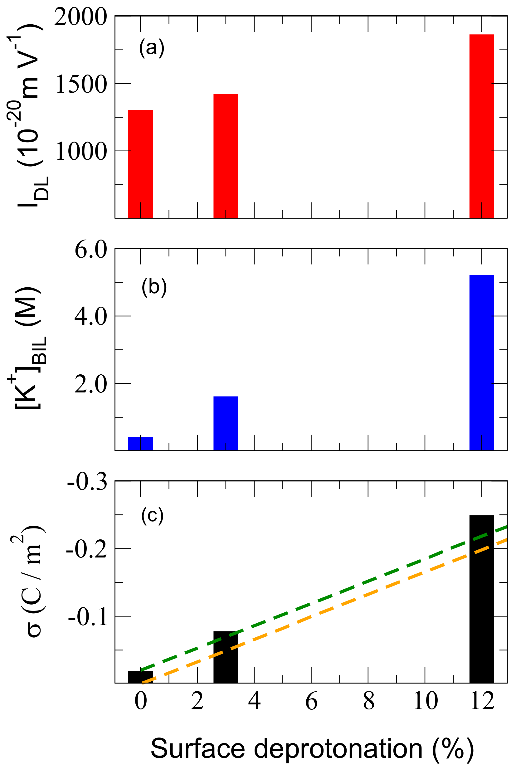
We illustrate this issue in Figure 4a where $I_{DL}$ from DFT-MD simulations on three hydroxylation states of the quartz surface is reported as a function of the surface deprotonation state (0%, 3% and 12%, see Table 1). It is important to stress that despite having only three points in this plot, they do cover a vast range of pH values for QW interfaces, approximatively between pH = 2 and pH = 10, according to ref. [34]. The $I_{DL}$ linear curve from theoretical SFG spectra obtained here as a function of the quartz surface degree of hydroxylation hence provides a way to experimentally extract the pH conditions for which the above-mentioned degree of hydroxylation is found at the quartz surface directly from experimental SFG spectra. By measuring Im${\chi }_{DL}^2\left(\omega \right)$ and its integral, $I_{DL}$, from SFG experiments performed under various pH conditions, one can indeed find the pH value for which the measured $I_{DL}$ is equal to the one calculated here in between 0% and 12% deprotonation of the oxide surface.

3.4. ${\chi }_{DL}^{\left(2\right)}\left(\omega \right)$: A Measure of the Surface Charge

We now show how to use Im${\chi }_{DL}^{\left(2\right)}\left(\omega \right)$ in conjunction with Im${\chi }_{BIL}^{\left(2\right)}\left(\omega \right)$ in order to reveal the screening of the surface charge and hence, reveal the electrolytic conditions in order to reach the isoelectric point at any aqueous interface, again using a synergy of SFG experiments and simulations. Generally speaking, experimentally and in DFT-MD simulations, one can increase the concentration of electrolytes in the aqueous solution (and hence, in the BIL) up to the point that the ionic concentration will be such that it can screen the surface charge at a given fixed pH condition. When the surface charge screening is reached, Im${\chi }_{DL}^{\left(2\right)}\left(\omega \right)$ and $I_{DL}$ are equal to zero—this is the isoelectric point.

This is easily done with MD simulations, and this is illustrated in Figure 4b for DFT-MD simulations run at three chosen hydroxylation states of the quartz surface (0%, 3% and 12% deprotonation state of the surface, all surfaces are, hence, negatively charged, see previous text and computational details) with various amounts of KCl electrolytic concentrations (see Table 1). Figure 4b reports an excess concentration of K${}^{+}$ cations located in the BIL necessary to completely screen the negative surface charge and achieve $I_{DL}=0$ (isoelectric point). The values are [K${}^{+}$]${}_{BIL}$ = 0.4, 1.6, 5.2 M, respectively, for the 0%, 3% and 12% deprotonation (dehydroxylation) states of the quartz surface. At these concentrations, Im${\chi }_{DL}^{\left(2\right)}\left(\omega \right)$ and $I_{DL}$ are indeed found equal to zero, hence providing the electrolytic concentration needed to reach the isoelectric point for each hydroxylation state of the quartz surface investigated here.

Interestingly, a very large K${}^{+}$ cation concentration in the BIL of 5.2 M is needed in order to reach the isoelectric point at the most deprotonated quartz surface (12% dehydroxylation). This is a very large ionic concentration needed to completely suppress the existence of the DL and hence, suppress bulk third-order contributions to SFG spectroscopy (i.e., suppress the bulk third-order contributions to DL-SFG related to the bulk-like organisation of water in the DL, with ${\chi }_{DL}^2\left(\omega \right)={\chi }_{DL}^3\left(\omega \right)\Delta {\varphi }_{DL}$, with $\Delta {\varphi }_{DL}=0$ at the isoelectric point). It is also important to note that the excess ionic concentration in the BIL is the only relevant quantity; the respective structural arrangement of anions/cations within the BIL and DL are irrelevant for the extraction of the isoelectric point at which ${\chi }_{DL}^{\left(2\right)}\left(\omega \right)$ and $I_{DL}$ are zero.

Once again, the information obtained from MD simulations is complementary to the knowledge provided by SFG experiments, which, with a similar approach, can reveal the nominal electrolytic concentration in the bulk at the isoelectric point. By comparing experiments and simulations, the excess ionic concentration in the BIL (i.e., at the surface) corresponding to a given value of (nominal) bulk concentration can be thus revealed, allowing direct characterization of the enrichment in ions at aqueous interfaces.

In the SFG experiments, one can indeed measure Im${\chi }_{DL}^{\left(2\right)}\left(\omega \right)$ and plot $I_{DL}$ as a function of the aqueous electrolyte concentration, for a given fixed pH condition. One will find a decreasing function that tends towards a plateau at the higher ionic concentrations, oscillating around $I_{DL}=0$. These oscillations are due to the Im${\chi }_{BIL}^{\left(2\right)}\left(\omega \right)$ SFG signal not being constant at all concentrations (there are changes in the BIL structure with increasing ionic excess concentration in the BIL), and especially, at the larger concentrations required to reach the isoelectric point. By increasing the electrolytic concentration in the aqueous phase, at a given fixed pH, the screening by the cations (here, at the illustrative quartz surface used in our examples) progressively suppresses the surface (negative) field/charge and hence, progressively suppresses the existence of the DL contribution to SFG. The onset of a (zero) plateau in the $I_{DL}$ function of the (nominal) aqueous electrolyte concentration represents the nominal concentration of electrolytes in the solution needed to reach the isoelectric point.

At this point, only the nominal concentration of electrolytes in the solution is known from experiments alone. However, we have just revealed above that there is a direct relationship between the aqueous electrolytic concentration and the excess concentration in the BIL, and this relationship is known from (DFT-)MD simulations. At the isoelectric point ($I_{DL}=0$), the enrichment in ions at the direct interface (i.e., in the BIL) is now simply given by [excess]${}_{BIL}$/[electrolyte]${}_{liquid}$. This relationship can obviously be applied at any $I_{DL}$ value; it is not restricted to the $I_{DL}=0$ isoelectric point. One has, indeed, to search for the common value of $I_{DL}$ in SFG experiments and in DFT-MD simulations at which point the electrolytic concentrations in the bulk (experiment) and the excess concentration at the interface (simulations) are then known. Note also that $I_{DL}=0$ is the only electrolytic condition for which interferences are not present in the SFG experimental signal.

Once the isoelectric point has been revealed, the total charge in the BIL, i.e., at the interface, is known and is equal to zero, by construction. The total electrolyte charge in the BIL is thus strictly opposite to the surface charge, therefore providing knowledge of the surface charge. The surface charge, $\sigma$ (in C/m${}^2$), is obviously given by $\sigma =-\frac{+q_{+}<N_{+}{>}_{BIL}-q_{-}<N_{-}{>}_{BIL}}{AB}$, where $q_{+}$ ($q_{-}$) is the cation (anion) charge; $<N_{+}{>}_{BIL}$ ($<N_{-}{>}_{BIL}$) is the average number of cations (anions) located in the BIL; and $AB$ is the surface area.

This is presented in Figure 4c, where the $\sigma$ values extracted from the above method are compared to the values obtained with Dove’s model [34] for silica oxides. Following the orange dotted line derived from Dove’s model and the $\sigma$ values extracted from our DFT-MD simulations, one can immediately see an excellent agreement, although Dove’s surface charges are systematically slightly lower than ours (by −0.019 C/m${}^2$). Dove’s model assumes that SiOH groups do not contribute to the surface charge, while we showed in ref. [14,28] and repeatedly through this text, that the neat fully hydroxylated quartz surface bears a negative charge because of the specific intertwined structure of the in-plane and out-of-plane orientations of the O–H terminations and surface polarization/charge transfer with water molecules H-bonded to the surface [14,28]. The resulting surface charge at the neat quartz–water interface is calculated here with the above-mentioned method to be $\sigma =-$0.019 C/m${}^2$. If one translates Dove’s $\sigma$ values by $\sigma =-$0.019 C/m${}^2$, one obtains the green dashed line in Figure 4c which provides surface quartz charges that are in even better quantitative agreement with the DFT-MD values—within 6%. Our method has, furthermore, the advantage of not needing any a priori knowledge of the surface sites’ pKa in order to estimate the surface charge.

It is worth adding a few more comments at this stage. The strategies proposed above for the surface charge determination bypass two well-known weaknesses of the MD simulations (DFT-MD and force field MD). One of these weaknesses, already mentioned, is the control of the pH in the simulation. It is largely unknown and very complicated to impose the “right” electrolytic concentration in the simulation box because of box size limitations (DFT-MD and force field MD alike). On the other hand, it is still non-trivial to perform constant pH simulations. A second weakness of DFT-MD and force field MD alike (although FF-MD is better in that respect) is the required configurational exhaustive sampling required in order to get a complete description of the electrolytic arrangements in the solution, in the DL, and in the BIL. One other issue is that the surface charge could certainly be extracted from ab initio static calculations on chosen or average interfacial electrolytic configurations. This, however, requires decomposition, localisation, and partitioning schemes, in order to go from wavefunction to atomic charges to the surface charge. It is well-known that the absolute charge values depend on the applied schemes, making this a non-trivial technique to get the absolute value of the surface charge.

4. Conclusions

In the present work, we showed that the non-linear SFG signal contained in the water Diffuse Layer (DL) is a powerful tool that can be used to reveal numerous essential properties of interfaces (solid–water and air–water alike). We showed that the Im${\chi }_{DL}^2\left(\omega \right)$ signal typically contains information about the surface potential and surface charge, the isoelectric point, the EDL (Electric Double Layer) formation at electrolytic interfaces, and the nominal pH of the solution and its relationship with the surface hydroxylation/protonation state. Note that all of these properties require phase resolved/heterodyne SFG, i.e., knowledge of Im${\chi }_{DL}^2\left(\omega \right)$. The standard/homodyne $|{\chi }_{DL}^2{\left(\omega \right)|}^2$ SFG signal lacks information on the sign of the potential across the DL, which would impede the extraction of the properties discussed in the present work.

In their work, Tian et al. [15] demonstrated that interfaces are composed of three water regions, namely, the BIL (Binding Interfacial Layer), the DL (Diffuse Layer), and Bulk water. Only the BIL and DL are non-centrosymmetric and hence, SFG-active, such that the SFG signal recorded at any charged interface has to be decomposed into Im${\chi }_{BIL}^2\left(\omega \right)$ and Im${\chi }_{DL}^2\left(\omega \right)$ in order to unravel the detailed microscopic organisation of water at charged aqueous interfaces. In their seminal work, the authors provided a strategy to extract Im${\chi }_{DL}^2\left(\omega \right)$ and hence , Im${\chi }_{BIL}^2\left(\omega \right)$, from the total recorded Im${\chi }^2\left(\omega \right)$ SFG signal. This strategy is based on a few assumptions and on the use of a model for the electric field. One has, furthermore, to correct the experimental SFG signal for interference effects, and one can follow refs. [16,17] to that end. In ref. [11], we subsequently showed how to unambigously extract these three regions of water at any charged aqueous interface from DFT-based molecular dynamic simulations. We remind the reader that our methodology is not restricted to DFT-MD but is applicable to any MD representation.

Both experiments and simulations hence provide the means to separate the Im${\chi }_{DL}^2\left(\omega \right)$ and Im${\chi }_{BIL}^2\left(\omega \right)$ of the DL and BIL regions of any charged interface, and hence, provide the means to use these signals to dissect the microscopic organisation of water at charged interfaces as well as provide the means to measure macroscopic properties of charged interfaces. The point we make in the present work is that Im${\chi }_{DL}^2\left(\omega \right)$ contains a wealth of information on the water microscopic organisation at the interface, which is highly complementary to the information that one would expect from the Im${\chi }_{BIL}^2\left(\omega \right)$ signal that reflects the organisation of the water in direct contact with the surface.

The first example given was direct measurement of the surface electric potential, i.e., the potential across the DL ($\Delta {\varphi }_{DL}$), which is given by the universal linear function of Figure 2. Using this figure, by experimentally measuring Im${\chi }_{DL}^2\left(\omega \right)$ and its integral, $I_{DL}$, in the O–H stretching spectral domain, one readily gets $\Delta {\varphi }_{DL}$, without the need for an electric potential model. Alternatively, one can extract Im${\chi }_{DL}^2\left(\omega \right)$ (and $I_{DL}$) from a DFT-MD simulation and, using Figure 2, one gets $\Delta {\varphi }_{DL}$ without further computationally expensive calculations of the ab initio electrostatic potential. The direct consequence is that the isoelectric point of the surface is directly accessible from Im${\chi }_{DL}^2\left(\omega \right)$—two measures (or simulations) only are needed to that end.

The second example given here was the knowledge of the formation of an EDL (Electric Double Layer) at charged interfaces directly from the Im${\chi }_{DL}^2\left(\omega \right)$ signal. With this demonstration, we showed that where the Im${\chi }_{BIL}^2\left(\omega \right)$ signal cannot reveal an EDL, the signal from the DL contains the information. We hence gave the protocol that experimentalists can apply to their recorded Im${\chi }_{DL}^{\left(2\right)}\left(\omega \right)$ signals to compare the neat interface signal and the signal at the electrolytic interface, without the need to systematically resort to computational simulations.

We furthermore showed that the Im${\chi }_{DL}^2\left(\omega \right)$ signal provides a direct measure of the aqueous (nominal) pH and its relationship to the surface charge state (i.e., hydroxylation state), which, in turn, can directly provide the surface charge. To obtain this information, one has to combine a few experiments and simulations—the former, indeed, carry the knowledge of nominal electrolyte pH, while the latter carry the knowledge of surface hydroxylation state. By combining measured and simulated Im${\chi }_{DL}^2\left(\omega \right)$ signals, one can obtain the desired pH–surface hydroxylation state relationship. The surface charge can hence be known without any (approximate) model.

For this, as well as for the unraveling of the excess ion concentration in the BIL, the theoretical results are not functional (for the DFT-MD simulations) and/or force field (in classical force field MD simulations) dependent, neither are they dependent on sampling (and time-length). The structural arrangement of the electrolytes and therefore, of the excess ions that are located in the BIL, is imposed (here, the initial conformation of the dynamics and the rather short time-scales of the DFT-MD do not modify this arrangement, but they could also easily be constrained in space in order to be maintained for much longer time-scale simulations, as could be achieved in classical MD). The DL-SFG intensity originating from each ionic distribution can be calculated, following decomposition into BIL-SFG and DL-SFG signals, which was developed in the present work. The experimental DL-SFG signals obtained for various nominal ionic concentrations in the Bulk layer can be compared to the calculated DL-SFG for given ionic distributions in the BIL, and from the experiment/calculation comparison, one can achieve the final knowledge of the ion propensity in the BIL and its relationship with the bulk ionic concentration, as shown in this work. The method presented here therefore overcomes the sampling limitations of MD simulations (AIMD and classical MD) as well as DFT functional/force field limitations.

We believe the protocols given in this work for both experimentalists and theoreticians will be applied and used broadly in the near future, giving rise to improved and more definitive interpretations of non-linear SFG (phase-resolved, heterodyned) signals.

References

- Laskin, A.; Gaspar, D.J.; Wang, W.; Hunt, S.W.; Cowin, J.P.; Colson, S.D.; Finlayson-Pitts, B.J. Reactions at Interfaces as a Source of Sulfate Formation in Sea Salt Particles. Science 2003, 301, 340–344. [Google Scholar] [CrossRef] [PubMed]
- Finlayson-Pitts, B.J.; Pitts, J.N. Chemistry of the Upper and Lower Atmosphere; Academic Press: Cambridge, MA, USA, 2000. [Google Scholar]
- Finlayson-Pitts, B.J. Atmospheric Chemistry. Proc. Nat. Acad. Sci. USA 2010, 107, 6566–6567. [Google Scholar] [CrossRef] [PubMed] [Green Version]
- Dawson, M.; Varner, M.E.; Perraud, V.; Ezell, M.J.; Gerber, R.B.; Finlayson-Pitts, B.J. Simplified mechanism for new particle formation from methanesulfonic acid, amines, and water via experiments and ab initio calculations. Proc. Nat. Acad. Sci. USA 2012, 109, 18719–18724. [Google Scholar] [CrossRef] [PubMed] [Green Version]
- Zhang, L.; Yang, Y.; Kao, Y.-T.; Wang, L.; Zhong, D. Protein Hydration Dynamics and Molecular Mechanism of Coupled Water—Protein Fluctuations. J. Am. Chem. Soc. 2009, 131, 10677–10691. [Google Scholar] [CrossRef] [PubMed]
- Lagi, M.; Lo Nostro, P.; Fratini, E.; Ninham, B.W.; Baglioni, P. Insights into Hofmeister Mechanisms: Anion and Degassing Effects on the Cloud Point of Dioctanoylphosphatidylcholine/Water Systems. J. Phys. Chem. B 2007, 111, 589–597. [Google Scholar] [CrossRef] [PubMed]
- Griffith, E.C.; Vaida, V. In situ observation of peptide bond formation at the water-air interface. Proc. Natl. Acad. Sci. USA 2012, 109, 15697–15701. [Google Scholar] [CrossRef] [PubMed] [Green Version]
- Malin, J.N.; Holland, J.G.; Saslow, S.A.; Geiger, F.M. U(VI) Adsorption and Speciation at the Acidic Silica/Water Interface Studied by Resonant and Nonresonant Second Harmonic Generation. J. Phys. Chem. C 2011, 115, 13353–13360. [Google Scholar] [CrossRef]
- Hayes, P.L.; Malin, J.N.; Konek, C.T.; Geiger, F.M. Interaction of Nitrate, Barium, Strontium and Cadmium Ions with Fused Quartz/Water Interfaces Studied by Second Harmonic Generation. J. Phys. Chem. A 2008, 112, 660–668. [Google Scholar] [CrossRef] [PubMed]
- Pezzotti, S.; Galimberti, D.R.; Gaigeot, M.-P. 2D H-Bond Network as the Topmost Skin to the Air-Water Interface. J. Phys. Chem. Lett. 2017, 8, 3133–3141. [Google Scholar] [CrossRef] [PubMed]
- Pezzotti, S.; Galimberti, D.R.; Shen, Y.R.; Gaigeot, M.-P. Structural definition of the BIL and DL: A new universal methodology to rationalize non-linear χ(2)(ω) SFG signals at charged interfaces, including χ(3)(ω) contributions. Phys. Chem. Chem. Phys. 2018, 20, 5190–5199. [Google Scholar] [CrossRef] [PubMed]
- Pezzotti, S.; Serva, A.; Gaigeot, M.-P. 2D-HB-Network at the air-water interface: a structural and dynamical characterization by means of ab-initio and classical molecular dynamics simulations. J. Chem. Phys. 2018, 148, 174701–174710. [Google Scholar] [CrossRef] [PubMed]
- Serva, A.; Pezzotti, S.; Bougueroua, S.; Galimberti, D.R.; Gaigeot, M.-P. Combining ab-initio and classical molecular dynamics simulations to unravel the structure of the 2D-HB-network at the air-water interface. J. Mol. Struct. 2018, 1165, 71–78. [Google Scholar] [CrossRef]
- Sulpizi, M.; Gaigeot, M.-P.; Sprik, M. The Silica-Water Interface: How the Silanols Determine the Surface Acidity and Modulate the Water Properties. J. Chem. Theory Comput. 2012, 8, 1037–1047. [Google Scholar] [CrossRef] [PubMed]
- Wen, Y.-C.; Zha, S.; Liu, X.; Yang, S.; Guo, P.; Shi, G.; Fang, H.; Shen, Y.R.; Tian, C. Unveiling Microscopic Structures of Charged Water Interfaces by Surface-Specific Vibrational Spectroscopy. Phys. Rev. Lett. 2016, 116, 016101. [Google Scholar] [CrossRef] [PubMed] [Green Version]
- Gonella, G.; Lutgebaucks, C.; de Beer, A.G.F.; Roke, S. Second Harmonic and Sum-Frequency Generation from Aqueous Interfaces is Modulated by Interference. J. Phys. Chem. C 2016, 120, 9165–9173. [Google Scholar] [CrossRef]
- Ohno, P.E.; Saslow, S.A.; fei Wang, H.; Geiger, F.M.; Eisenthal, K.B. Phase-referenced Nonlinear Spectroscopy of the alpha-Quartz/Water Interface. Nat. Commun. 2016, 7, 13587–13591. [Google Scholar] [CrossRef] [PubMed]
- Ohno, P.E.; Wang, H.-f.; Geiger, F.M. Second-order spectral lineshapes from charged interfaces. Nat. Commun. 2017, 8, 1032. [Google Scholar] [CrossRef] [PubMed] [Green Version]
- Joutsuka, T.; Hirano, T.; Sprik, M.; Morita, A. Effects of third-order susceptibility in sum frequency generation spectra: A molecular dynamics study in liquid water. Phys. Chem. Chem. Phys. 2018, 20, 3040–3053. [Google Scholar] [CrossRef] [PubMed]
- Joutsuka, T.; Morita, A. Electrolyte and Temperature Effects on Third-Order Susceptibility in Sum-Frequency Generation Spectroscopy of Aqueous Salt Solutions. J. Phys. Chem. C 2018, 122, 11407–11413. [Google Scholar] [CrossRef]
- Hutter, J.; Iannuzzi, M.; Schiffmann, F.; VandeVondele, J. cp2k: Atomistic simulations of condensed matter systems. WIREs Comput. Mol. Sci. 2014, 4, 15–25. [Google Scholar] [CrossRef] [Green Version]
- VandeVondele, J.; Krack, M.; Mohamed, F.; Parrinello, M.; Chassaing, T.; Hutter, J. Quickstep: Fast and accurate density functional calculations using a mixed Gaussian and plane waves approach. Comput. Phys. Commun. 2005, 167, 103–128. [Google Scholar] [CrossRef] [Green Version]
- Becke, A.D. Density-functional exchange-energy approximation with correct asymptotic behavior. Phys. Rev. A 1988, 38, 3098–3100. [Google Scholar] [CrossRef]
- Lee, C.; Yang, W.; Parr, R.G. Development of the Colle-Salvetti correlation-energy formula into a functional of the electron density. Phys. Rev. B 1988, 37, 785–789. [Google Scholar] [CrossRef]
- Goedecker, S.; Teter, M.; Hutter, J. Separable dual-space Gaussian pseudopotentials. Phys. Rev. B 1996, 54, 1703–1710. [Google Scholar] [CrossRef] [Green Version]
- Grimme, S. Accurate description of van der Waals complexes by density functional theory including empirical corrections. J. Comput. Chem. 2004, 25, 1463–1473. [Google Scholar] [CrossRef] [PubMed]
- Grimme, S. Semiempirical GGA-type density functional constructed with a long-range dispersion correction. J. Comput. Chem. 2006, 27, 1787–1799. [Google Scholar] [CrossRef] [PubMed]
- Pfeiffer-Laplaud, M.; Gaigeot, M.-P. Electrolytes at the Hydroxylated (0001) α-Quartz/Water Interface: Location and Structural Effects on Interfacial Silanols by DFT-Based MD. J. Phys. Chem. C 2016, 120, 14034–14047. [Google Scholar] [CrossRef]
- Pfeiffer-Laplaud, M.; Gaigeot, M. Adsorption of Singly Charged Ions at the Hydroxylated (0001) α-Quartz/Water Interface. J. Phys. Chem. C 2016, 4866–4880. [Google Scholar] [CrossRef]
- Morita, A.; Hynes, J.T. A Theoretical Analysis of the Sum Frequency Generation Spectrum of the Water Surface. II. Time-Dependent Approach. J. Phys. Chem. B 2002, 106, 673–685. [Google Scholar] [CrossRef]
- Morita, A.; Ishiyama, T. Recent progress in theoretical analysis of vibrational sum frequency generation spectroscopy. Phys. Chem. Chem. Phys. 2008, 10, 5801–5816. [Google Scholar] [CrossRef] [PubMed]
- Khatib, R.; Backus, E.H.G.; Bonn, M.; Perez-Haro, M.-J.; Gaigeot, M.-P.; Sulpizi, M. Water orientation and hydrogen-bond structure at the fluorite/water interface. Sci. Rep. 2016, 6, 24287. [Google Scholar] [CrossRef] [PubMed] [Green Version]
- Skinner, S.A.C.J.L. Infrared and Raman Line Shapes of Dilute HOD in Liquid H2O and D2O from 10 to 90 ∘C. J. Phys. Chem. A 2005, 109, 6154–6165. [Google Scholar]
- Dove, P.M. The dissolution kinetics of quartz in sodium chloride solutions at 25 ∘C to 300 ∘C. Am. J. Sci. 1994, 294, 665–712. [Google Scholar] [CrossRef]
Figure 1.
Calculated Im and Re of the DL (Diffuse Layer) of the (0001) -quartz–liquid water interface (QW) under various chemical conditions: QW is the fully hydroxylated aqueous surface, “QW + x% dep” are deprotonated states of the aqueous surface (hence representing varied pH conditions), and “QW xM [K]” are fully hydroxylated aqueous surfaces with varied excess cation concentrations located in the BIL ([K]= 1.6 M, 4.2 M and 7.1 M), the anions of the KCl electrolyte being located in the DL.
Figure 2.
Evolution of the electrostatic potential across the DL () as a function of (integral of Im in the 3000–3600 cm region). The black points are the calculated values from the DFT-MD simulations of the various silica–water interfaces for which SFG spectra are plotted in Figure 1; the red line passes through all calculated points.
Figure 3.
(A) Calculated Im spectra for a KCl electrolytic (0001) -quartz interface (1 KCl vs. 518 water molecules in the simulation box), where the surface oxide is dehydroxylated by 3% (denoted “3% dep” in the text and figures). Two possible ionic arrangements were considered: either both ions are simultaneously located in the BIL (in blue), or K located in the BIL while Cl is in the DL (in red). (B) Calculated Im spectra for a KCl electrolytic air–water interface (here DO, 1 KCl vs. 256 water molecules in the simulation box). The two possible ionic arrangements are either both ions located simultaneously in the BIL (in blue), or Cl is in the BIL while K is in the DL (in red). For (A,B), the total Im spectra (TOT) of the interfaces are presented at the top, the Im spectra of the BIL water layer are presented in the middle, the Im spectra of the BIL water layer are presented below, and the Im spectra of the bulk liquid water (the rest of the water layers at the interfaces) are presented at the bottom. Schematic representations of the ion positions in BIL/DL for the four configurations are also presented. The colors surrounding the schemes (blue/red) refer to the color coding of two ions located simultaneously in the BIL (blue, no-Electric Double Layer (EDL)) and two ions dispatched inbetween the BIL and DL (red, EDL).
Figure 4.
(a) values obtained for (0001) -quartz–water interfaces with an increasing degree of surface deprotonation (dehydroxylation). (b) Excess [K] concentration in the BIL needed to bring the QW interfaces at the isoelectric point. (c) Surface charge, , calculated from the simulated Sum Frequency Generation (SFG) spectra of the QW interfaces at increasing surface deprotonation/dehydroxylation and compared to previous extimations from ref. [34] (orange dashed line) and to the values obtained form ref [34] once correcting for the negative contribution of SiOH to the surface charge (dashed green line, see discussion in the text).