New Outlier Top-Cut Method for Mineral Resource Estimation via 3D Hot Spot Analysis of Borehole Data


1
Division of Graduate Education for Sustainability of Foundation Energy, Seoul National University, Seoul 08826, Korea
2
Department of Energy Resources Engineering, Pukyong National University, Busan 48513, Korea
3
Department of Energy Resources Engineering, Seoul National University, Seoul 08826, Korea
*
Author to whom correspondence should be addressed.
Minerals 2018, 8(8), 348; https://doi.org/10.3390/min8080348
Submission received: 18 July 2018
/
Revised: 31 July 2018
/
Accepted: 9 August 2018
/
Published: 11 August 2018
Abstract
:Three-dimensional (3D) analysis of borehole data is very important for effective mineral exploration. It can be used not only to understand the geological structure of the underground, but to estimate the amount of the resource. In the mining industry, the geostatistical interpolation, such as kriging, is widely used to predict the value of a whole section using this borehole data. In order to obtain reasonable prediction results, it is firstly necessary to verify assay and geological databases. In addition, if the assayed grade data deviates significantly from the average value, it is necessary to perform the prediction including the outlier top-cut because it may excessively affect the predicted value. However, the existing top-cut methods of determining a specific threshold value may cause an error by excluding significant data. In this study, to minimize the loss of such data, we developed a 3D hot spot analysis technique to analyze statistically significant outliers. In addition, it was applied to borehole data analysis of the Au deposit. As a result, we confirmed that the proposed method can mitigate the overestimation or underestimation that might occur when applying the existing methods.
1. Introduction
Resource estimation based on computerized methods has been widely used in the mining industry. This method is fast and editable compared to the traditional manual methods. Today, three-dimensional (3D) terrain modeling software, such as Micromine (Micromine, Perth, Australia), GOCAD (Paradigm, Houston, TX, United States), GEMS (Dassault Systèmes, Vélizy-Villacoublay, France) and Surpac (Dassault Systèmes, Vélizy-Villacoublay, France), can integrate two-dimensional (2D) geographic information systems (GIS), databases, statistical methods, and 3D visual technologies. Complex and irregular geological objects in this software can be modeled in a 3D environment using a variety of data sources such as topographic maps, geophysical data, and geochemical data [1,2].
For the application of computerized methods, 3D modeling of the ore body as a geological basis should be done through stratum analysis and critical review of existing sample data. Then, these envelopes can be divided into block models. The grade of the block is estimated by mathematical methods, such as geostatistical interpolation. However, the computerized method itself does not guarantee the quality of the results, and numerous mining projects modeled and designed using computerized methods have failed [3]. Because the geostatistical method is only a tool for estimating grades, it cannot solve the existing problems of assay databases or geological interpretations. Therefore, assay and geological databases should be verified before they are used for resource estimation. In addition, unbiased models are important for well-established geological resource assessments because biased model can result in resource overestimation.
To avoid the problem of overestimation, the outlier samples that do not conform to the distribution of the analysis should be appropriately capped. This process is called top-cut. The determination of the values considered as outliers is subjective. The high grade sample should be limited enough to prevent overestimation, but not too conservatively. There are some commonly used top-cut methods for determining the capping grade [4,5,6]. One way is to use a breakpoint on the log-normal cumulative frequency plot. If the assay sample follows a log-normal distribution, the data points of the probability plot must follow a straight line. In some cases, outliers are defined as values outside of a specific interval, such as 2 or 3 standard deviations from the mean or median of the distribution. Another common approach is to use the 95th percentile of cumulative frequency.
However, these methods cannot manage different types of outliers properly. Isolated outliers cause a problem in estimation because they tend to have different continuity than most of the data. Therefore, they must be treated differently. More abundant, clustered outliers may define a sufficiently large domain, which has spatial connectivity, and it can be considered as a significant mineralized area [7]. The presence of outliers is particularly problematic if they have minimal spatial connectivity [8]. In other words, there is a large potential impact of outliers on overestimation if they are located within a small, spatially restricted volume. Because clustered outliers can be a significant data source for mineralization, unlike isolated outliers, they should be managed differently. However, existing methods cannot separate them because they consider only the absolute value of the assayed data.
To overcome this limitation in defining outliers, this study proposed a new method by using hot spot analysis, which calculates z-scores based on the Getis–Ord Gi* statistic [9], identifying a statistically significant hot spot sample. To be a statistically significant hot spot, a feature will have a high value and be surrounded by other features with high values. This method has been widely used in applied geographic research to identify clustering of species populations, diseases, and crime incidence. Recently, there have been some studies to assess the soil contamination using hot spot analysis. McClintock [10] evaluated the risk of lead contamination at post-industrial landscapes in Oakland, California using hot spot analysis. Griffith et al. [11] considered location error impacts on local spatial autocorrelation by simulating significant heavy metal clusters using local Moran’s I and Getis–Ord Gi*. In addition, Kim et al. [12] supported soil survey planning by using hot spot analysis. However, previous studies of hot spot analysis were applied only to 2D data and there was no case applied to 3D spatial data, such as borehole data.
In this study, we developed a 3D hot spot analysis algorithm that can be used for borehole data, and separates clustered outliers and isolated outliers. In addition, kriging was applied for resource estimation considering the outliers. Kriging is a widely used geostatistical interpolation technique in the mining industry. The gold (Au) assay data from boreholes of Au deposits in the Cobre Panama district were used for analysis. The methods for handling outliers in estimating resources are also diverse and subjective, like the methods for outlier determination. For example, in order to reduce the influence of outlier data, a method can be used that reduces a value above a certain threshold value to the threshold value. Another method excludes outlier data from the analysis altogether. A method which excludes outliers in the variogram modeling process for analyzing the autocorrelation and uses them in the kriging prediction step can be an alternative. In this study, outliers are excluded from the analysis in all processes for resource estimation. However, unlike the isolated outliers, the clustered outliers may represent important mineralization, so the data are preserved and the results are compared to other outlier determination methods.
2. Materials and Methods
2.1. Study Area and Data
In order to apply the proposed method, the part of Colina Au deposit in the Cobre Panama district was targeted. In the area of the Cobre Panamá deposits, the oldest rocks are submarine andesite and basalt flows and tuffs, intercalated with clastic sedimentary rocks and reef limestone, of probable Eocene to early Oligocene age. Miocene and younger rocks comprise the bulk of volcanic rocks in western Panamá and consist of terrestrial and marine volcanic and volcanic-derived rocks of progressively more felsic composition. Copper-gold-molybdenum porphyry style mineralization occurs at the southern margin of a large granodiorite batholith of mid-Oligocene age. The three main deposits of the Cobre Panamá deposits are Botija, Colina, and Valle Grande [13]. Hydrothermal alteration is primarily silica-chlorite, which is interpreted to be a form of propylitic alteration [14,15].
The Colina deposit is a 2.5 km long and 1 km wide feldspar quartz hornblende porphyry sill and dike complex. An irregular L-shaped andesite roof pendant with the long axis orientated to the east-southeast and the short axis orientated to the south-southwest is located in the southern part of the deposit. The majority of the feldspar quartz hornblende porphyry comprises 50 m to 200 m thick sills that dip shallowly to the north and are often interconnected by dikes [13].
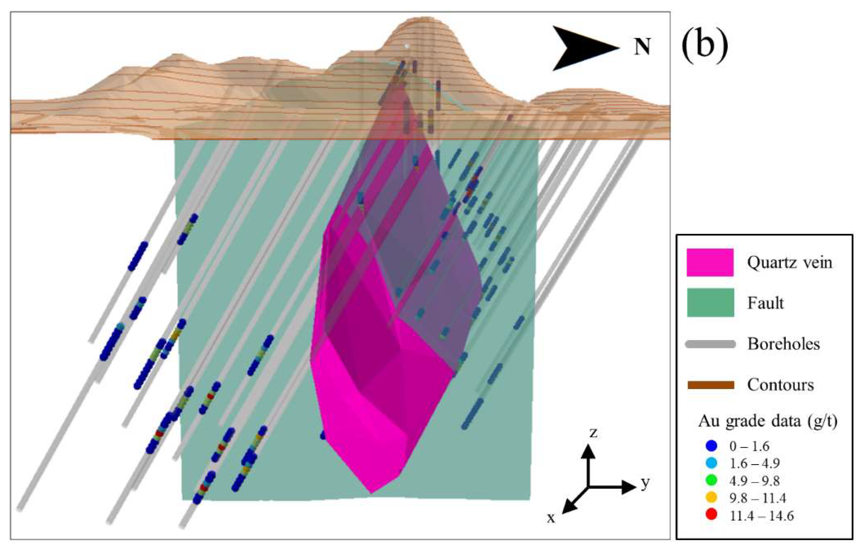
The study area is a part of Colina deposit. Approximately 1400 Au grade data from 52 boreholes were used, and this area is a region with a quartz vein with distributed Au, and a north-south direction displacement occurs adjacent to a fault. The 3D spatial database constructed in this study includes the borehole assay data, the contour lines showing the topographical relief, the fault, and the quartz vein. These data are visualized using ArcScene software (version 10.4, Environmental Systems Research Institute, Redlands, CA, United States), as shown in Figure 1. The vein, including Au, is in the form of plate quartz, and develops in the east-west direction with a slope in the 60–70° north direction. The domain of quartz vein was defined by the Korea Resources Corporation considering the fault and assayed borehole data. The near vertical fault is developed in the north-south direction. The 52 boreholes consisted of 10 vertical boreholes and 42 inclined boreholes (dip 60°, azimuth 180°).
The histogram from the Au grade assay data of the boreholes reveals a clear difference in Au grade between the quartz vein and the surrounding gangue (Figure 2). In other words, Au mineralization is dominated mainly by the quartz vein. Since there is little spatial correlation between the quartz vein and other regions, this study only analyzed data that corresponded to the quartz vein. Data compositing was performed as preprocessing of the data. Compositing is the process of averaging data within a specific length and converting it into samples of the same length. It has the advantage of reducing the amount of analytical data and providing the data at an even resolution in the assessment of resources [16,17]. In this study, compositing was performed at intervals of 3 m considering the intervals of assay data. Since the displacement occurred about 100 m from the fault after the formation of the vein, data on the east side of the fault was moved for hot spot analysis and kriging analysis by moving the relative position to the north by 100 m.
2.2. Hot Spot Analysis for Determining the Capping Grade
In order to distinguish between clustered outliers and isolated outliers, it is necessary to analyze the spatial correlation between the borehole data. There are several ways to test and measure spatial autocorrelation. Moran’s I, semivariance, and spatial autocorrelation coefficients are very popular methods. Although they are applied globally to the complete region of the study area, it is often required to examine the pattern at a more local scale. Getis and Ord [9] focused upon local effects and introduced a measure of spatial association called the Getis–Ord Gi* statistic.
In this study, the Getis–Ord Gi* statistic was calculated for each Au sample value in a borehole dataset by considering the 3D spatial coordinates of the borehole data. Since existing analysis tools, such as the hot spot analysis tool of ArcGIS, can only calculate values in 2D space, we developed a 3D hot spot analysis tool using Visual Basic 2013 (Microsoft Corporation, Washington, WA, United States) for 3D space analysis. The Getis–Ord Gi* statistic is calculated by comparing the local sum for a feature and its neighbors to the total sum as follows:
where xj is the attribute value for feature j, wi,j is the spatial weight between feature i and j, n is equal to the total number of feature and
The resultant statistic is a z-score. For statistically significant positive z-scores, the larger the z-score, the more intense the clustering of high values (i.e., hot spot). When the local sum is very different from the expected local sum, and that difference is too large to be the result of random chance, a z-score is statistically significant. In other words, a feature with a high value surrounded by other high value features is a statistically significant hot spot feature.
To determine the spatial weight wi,j between borehole data, four methods were applied in the developed 3D hot spot analysis tool. They are the inverse distance method, the inverse distance squared method, the fixed distance band method, and the zone of indifference method according to how spatial relationships among features are conceptualized. It is generally known that the fixed distance band method is a great option in choosing the right conceptualization of spatial relationships [18]. In the case of a fixed distance band method, the scale of analysis does not change across the study area because it uses a critical fixed distance to decide which neighbors to include. In this study, the hot spot analysis results using the fixed distance band method are presented for determining the outliers that should be excluded in the kriging prediction process.
To assess statistically significant clustered outliers, composited Au sample data were classified as four groups according to the Au grade and z-scores of the statistics. The four groups are as follows: high grade value with high z-score (HH), high grade value with low z-score (HL), low grade value with high z-score (LH), and low grade value with low z-score (LL). The grade value normalized by standard deviation and z-score were utilized as the x variable and y variable in a scatter plot to classify the dataset into four groups. According to the existing top-cut methods, higher values above a certain threshold value should all be excluded, but in this study, we proposed a method named hot spot top-cut that does not exclude clustered outliers when the z-score is high. A schematic diagram of the application of the proposed method for borehole data is shown in Figure 3.
2.3. Variography and Grade Estimation
Variography, or spatial statistics, is the determination of the spatial correlation of sample values. It is a very important study in the computerized resource estimation of the mining industry. If kriging is used for grade estimation, experimental variograms are very important as a preliminary analysis. The experimental variogram γ(h) measures the variability of two data pairs [] that are separated by lag vector h, as follows:
where N is the number of data pairs for a particular distance and direction. After comprehending the spatial correlations of the data from the experimental variogram, the theoretical variogram should be modeled well as a representative of the experimental variogram to compute these correlations over all distances.
One of the most common problems in variogram modeling occurs when a variogram calculation is not limited to mineralized samples. If the assay samples are mixed with mineralized and waste samples, they are strongly influenced by low grade waste samples in the variogram calculation [3]. That is, a seemingly good and smooth variogram model with a long variogram range can be computed, but it yields inadequate conclusions with irrational long distance correlations. To prevent this, it is necessary to perform calculations by distinguishing geological domains. Another method is to set the cut-off grade and exclude the value below the grade for the variogram calculation.
One of the most popular methods in geostatistics is kriging. Kriging is a technique for predicting values for unknown points using a weighted linear combination of known values (Equation (5)).
Here, denotes the kriging prediction value for the prediction point, and denotes the known surrounding values. represents the weight of each data, and N represents the total number of data used for kriging prediction. There are several types of kriging according to the difference in the process of determining the weights. Among them, ordinary kriging and indicator kriging are the most commonly used methods in the mining industry grade estimation.
Ordinary kriging does not bias the prediction equation and minimizes the error variance. At this time, the sum of the weights of the samples equals 1. It has been proved that the result is stable in the grade estimation and widely used in the mining industry [19,20,21]. Indicator kriging converts the grade of the sample to the indicators of a 0 or 1 based on the cut-off grade prior to the variogram modeling. This method does not predict the grade of the block, but evaluates the possibility that the grade of the block is higher than the selected cut-off grade [22,23]. The purpose of this study is to evaluate the applicability of the proposed hot spot top-cut method for grade estimation. Therefore, ordinary kriging was chosen—the most popular spatial interpolation method in grade estimation.
3. Results and Discussion
3.1. Outlier Determination
We applied the existing methods for determining outliers and compared them to the proposed method. Figure 4 shows the method of determining the outliers by using the probability plot, and the Au grade of 12.15 g/t, in which the slope change is determined as the threshold value of the outlier. In addition, when the upper 5% value is used as the threshold value, the grade of 13.37 g/t is determined as the top-cut value. When +2 standard deviations of the mean is applied, the grade of 14.29 g/t is determined as the threshold value. In the following, each top-cut method in the text is called prob (probability) top-cut, perc (95% percentile) top-cut, and std (+2 standard deviations) top-cut. In these methods, if the absolute value is above the threshold for top-cut, they are all evaluated as the same outlier, and the values determined by the respective methods are shown on the probability plot (Figure 4). In order to overcome the limitations of these methods, the data classification by applying the proposed method is shown in Figure 5a. The large red circle represents a clustered outlier where the Au grade is very high as the top 5%, and the z-score is also high as the top 10%. On the other hand, a large yellow circle represents a relatively isolated outlier where the Au grade is high as the top 5%, but the z-score is less than the top 10%. The classification results are displayed in three dimensions in Figure 5b. Large yellow circles are scattered relatively sporadically, whereas large red circles are densely distributed.
3.2. Variogram Modeling and Kriging Analysis
Figure 6 shows the results of the experimental variogram analysis and theoretical variogram modeling for all borehole data or capped data by the respective top-cut method, which is required to perform spatial interpolation by using ordinary kriging. The variogram modeling was performed in SGeMS software (version 2.1b, Stanford University, Stanford, CA, United States), which is an open-source computer package for solving problems involving spatially related variables. An exponential model was selected as a fitting function for the theoretical variogram model. Since the remaining data are the same, except for the capped data, the overall trend of each variogram is similar. The nugget value and the range were all applied equally, and the range value was set to 100 m. When all data are used (Figure 6a), the sill value is the largest, and the lower the threshold value of the outlier, the smaller the sill value because the variation of Au grade values is minimal. The distribution of mineral deposits and Au grades can be anisotropic and variograms can be different, depending on dips and directions. However, the purpose of this study is to evaluate the difference between the proposed method and the existing top-cut methods for grade estimation. Therefore, an omnidirectional model was considered assuming the isotropy for the control of the variables.
Ordinary kriging was applied for estimating the Au grades of the quartz vein. The highest predicted values are widely distributed in the case of using all data because all data including outliers are used for the kriging prediction (Figure 7a). In the case of top-cut using the probability plot, the outliers are capped the most because of the lowest threshold value. It can be seen that the distribution of high values at both ends and center of the quartz vein is considerably reduced (Figure 7b). In the case of applying top-cut using standard deviation, the threshold value is the highest, so the number of outliers excluded is the lowest and there is no significant difference in the distribution of predicted values with all data (Figure 7d). When the upper 5% value is capped, the result corresponds to the middle of the two top-cut methods mentioned above (Figure 7c). The predicted values at both ends of the quartz vein were lower compared to the case of using all data. Finally, in the case of applying the hot spot top-cut proposed in this study, the clustered western anomalies are maintained to some extent and the predicted values of the isolated eastern anomalies are predicted to be low (Figure 7e). Therefore, when applying the proposed hot spot top-cut method, it is possible to preserve the information of important mineralized areas in consideration of the spatial distribution, not merely by excluding the values with high absolute values.
3.3. Validation
To validate the estimation, it is necessary to evaluate whether the global mean of the estimated block grades and the data are identical. For this purpose, a histogram can be useful (Figure 8). Figure 8a shows the results of the kriging prediction using all the assay data, and Figure 8b–d shows the prediction results using the existing top-cut methods. Figure 8e corresponds to the histogram of kriging predictions using the hot spot top-cut method proposed in this study. Each of these histograms is the result for an estimated 26,676 blocks, whereas Figure 8f shows the histogram for 132 assay samples corresponding to the quartz vein. The overall trend of the histogram of kriging predictions is similar to the histogram of assay data, but both ends of the distribution are reduced by the smoothing effect due to the nature of the interpolation method [17]. Especially when the threshold value of the outlier is decreased by using the existing top-cut methods, it can be seen that the higher predicted values are decreased. In the std top-cut method (Figure 8d) with a large threshold value and the hot spot top-cut method (Figure 8e) considering clustered outliers, relatively high values are maintained in the prediction process. Table 1 shows the minimum, maximum, average, skewness, and total Au amount for each kriging prediction and assay data. The average value is most similar to the sample data when all data are utilized. On the other hand, the skewness is most different from the sample data. The total amount of Au in the vein was calculated by considering the volume of block (27 m3), number of blocks (26,676), density of rock (2.5 g/cm3), and average of predicted Au grade. Because one prediction method may not have the best results in all respects, it is necessary to approach and review various methods. In addition, the validity of the prediction cannot be verified by the global estimation result alone. Therefore, the verification of the local estimation is also necessary.
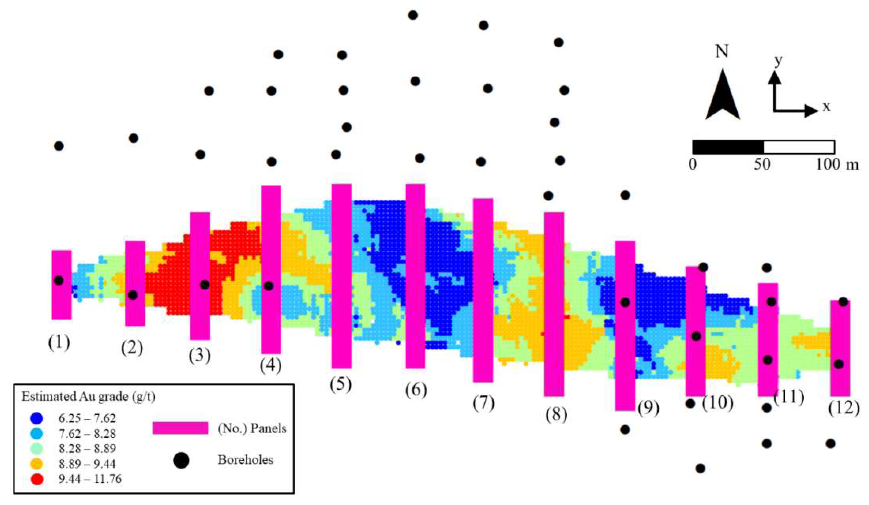
In order to verify the local predicted grade, a method of comparing the predicted value of the block and the borehole data for the panels traversing the entire ore body can be generally used. These panels are typically drawn along the strike of the ore body and contain one or more boreholes [24,25]. In this study, 12 panels were constructed, as shown in Figure 9, to include all borehole data and average grades were calculated for each panel. Table 2 shows the mean values of borehole data and kriging predictions for each panel. They are plotted on a line diagram against each panel (Figure 10). According to the smoothing effect of the kriging prediction, the value is predicted to be low in the part where the value of the borehole data is high and the value is predicted to be high in the part where the value of the borehole data is low [17]. This smoothing effect is a general phenomenon, but the smaller the degree, the better the prediction result. Although the result of using all data is most similar to the result of the borehole data, there is a risk of overestimation. Existing top-cut methods can underestimate panels 2–4 as the threshold value of the outlier decreases. In particular, the prob top-cut method with the lowest threshold value tends to underestimate Au grade as a whole. For panel 11, overestimation is prominent when using all data and the std top-cut method. It was confirmed that the hot spot top-cut method can mitigate the overestimation of panel 11 while evaluating panels 2–4 as a significant mineralized zone.
4. Conclusions
In this study, a 3D hot spot analysis technique for quantifying statistically significant data was developed and applied to borehole data analysis of the Au deposit. The resource estimation using kriging is very useful with the advancement of computer technology. However, the presence of outliers, which are much higher than other values, can lead to overestimation in the kriging prediction process, which can cause great problems in assessing the resources. In order to prevent the effect of overestimation, various top-cut methods are used to manage outliers in the analysis. However, existing methods have a limitation that they can consider only a certain threshold value.
Even if the outliers have the same grade value, the actual importance may be different depending on whether they are clustered outliers that are spatially connected or isolated outliers that do not have spatial connectivity. The isolated outliers may be the main cause of overestimation, while the clustered outliers may represent the important mineralization. Therefore, it is necessary to evaluate spatial density, that is, spatial statistical significance. The density of Au grade in 3D space is evaluated as the Getis–Ord Gi* statistic by applying the hot spot analysis method proposed in this study. In this study, a new top-cut method was proposed and applied to the Au grade data of the Au deposit. When using the existing top-cut methods, such as probe top-cut, perc top-cut, and std top-cut, Au grade data higher than a specific value was excluded in the kriging analysis. On the other hand, statistically significant hot spot data could be included by hot spot top-cut in the kriging analysis. As a result, we confirmed that it is possible to mitigate the overestimation or underestimation of a local area that might occur when applying the existing methods.
The results of this study can contribute to securing significant data in the prediction of resources using kriging. In the assessment of resources, the top-cut process has no established criteria and is subject to analyst discretion. The proposed hot spot top-cut method is also subject to evaluation depending on how the outlier threshold is determined and how the threshold value of the z-score is determined. However, it is possible to add an option for the analyst’s judgment, in that it provides a new field of view for areas that cannot be found by conventional methods. In this study, only the isotropy was considered for evaluating the correlation between data, but it is expected that the analytical application and accuracy will be improved if further anisotropy is considered in the future. Also, if the results are verified and the analysis method is improved by comparing it to the production amount, the proposed method will be more useful. The proposed method is expected to be applicable not only to underground data, but also to atmospheric and underwater data.
Author Contributions
Y.C. conceived and designed the experiments; S.-M.K. and Y.C. performed the experiments; S.-M.K. developed the software and analyzed the data; H.-D.P. contributed reagents/materials/analysis tools; and S.-M.K. and Y.C. wrote the paper.
Funding
This work was supported by (1) Basic Science Research Program through the National Research Foundation of Korea (NRF) funded by the Ministry of Education (2015R1D1A1A01061290), (2) the Brain Korea 21 Project, and (3) the Research Institute of Energy and Resources, Seoul National University, Korea.
Conflicts of Interest
The authors declare no conflicts of interest.
References
- Mallet, J.L. Geomodeling Applied Geostatistics Serie; Oxford University Press: New York, NY, USA, 2002. [Google Scholar]
- Zanchi, A.; Francescac, S.; Stefano, Z.; Simone, S.; Graziano, G. 3D reconstruction of complex geological bodies: Examples from the Alps. Comput. Geosci. 2009, 35, 49–69. [Google Scholar] [CrossRef]
- Bullock, R.L.; Mernitz, S. Mineral Property Evaluation: Handbook for Feasibility Studies and Due Diligence; Society for Mining, Metallurgy & Exploration: Englewood, NJ, USA, 2017. [Google Scholar]
- Valley, M.; David, M.; Dagbert, M.; Desrochers, C. Guide to the Evaluation of Gold Deposits; Geological Society of CIM: Calgary, AB, Canada, 1992. [Google Scholar]
- Sinclair, A.J. A fundamental approach to threshold estimation in exploration geochemistry: Probability graphs revisited. J. Geochem. Explor. 1991, 41, 1–22. [Google Scholar] [CrossRef]
- Parker, H.M. Statistical treatment of outlier data in epithermal gold deposit reserve estimation. Math. Geol. 1991, 23, 175–199. [Google Scholar] [CrossRef]
- Sinclair, A.J.; Garston, H.B. Applied Mineral Inventory Estimation; Cambridge University Press: Cambridge, UK, 2006. [Google Scholar]
- Rossi, M.E.; Clayton, V.D. Mineral Resource Estimation; Springer: Berlin, Germany, 2013. [Google Scholar]
- Getis, A.; Ord, J.K. The analysis of spatial association by use of distance statistics. Geogr. Anal. 1992, 24, 189–206. [Google Scholar] [CrossRef]
- McClintock, N. Assessing soil lead contamination at multiple scales in Oakland, California: Implications for urban agriculture and environmental justice. Appl. Geogr. 2012, 35, 460–473. [Google Scholar] [CrossRef]
- Griffith, D.A.; Chun, Y.; Lee, M. Locational Error Impacts on Local Spatial Autocorrelation Indices: A Syracuse Soil Sample Pb-Level Data Case Study. In Proceedings of the Spatial Accuracy Assessment in Natural Resources and Environmental Sciences, Montpellier, France, 5–8 July 2016. [Google Scholar]
- Kim, S.M.; Choi, Y. Assessing statistically significant heavy-metal concentrations in abandoned mine areas via Hot Spot Analysis of portable XRF data. Int. J. Environ. Res. Public Health 2017, 14, 654. [Google Scholar] [CrossRef] [PubMed]
- Rose, W.L.; Burge, C.; Davis, B.; Kozak, A.; Sim, R.; Wells, G.S. Mina De Cobre Panamá Project, Panamá, NI 43-101 Technical Report; Inmet Mining Corporation: Toronto, ON, Canada, 2010. [Google Scholar]
- Sepp, M.D.; John, H.D. Structural evolution, vein orientation, and paragenesis of the botija porphyry Cu-Mo-(Au) deposit, Panama. Econ. Geol. 2018, 113, 857–890. [Google Scholar] [CrossRef]
- Gray, D.; Lawlor, M.; Stone, R. Cobre Panamá Project, Colón Province, Republic of Panamá, NI 43-101 Technical Report; First Quantum Minerals Limited: Vancouver, BC, Canada, 2015. [Google Scholar]
- Pan, G. Practical issues of geostatistical reserve estimation in the mining industry. CIM Bull. 1995, 88, 31–37. [Google Scholar]
- Abzalov, M. Applied Mining Geology; Springer: Berlin, Germany, 2016. [Google Scholar]
- Environmental Systems Research Institute (ESRI). ArcGIS Desktop Help 10.2 How Hot Spot Analysis (Getis–Ord Gi*) works. Available online: http://resources.arcgis.com/en/help/main/10.2/index.html (accessed on 1 July 2018).
- Wang, G.; Huang, L. 3D geological modeling for mineral resource assessment of the Tongshan Cu deposit, Heilongjiang Province, China. Geosci. Front. 2012, 3, 483–491. [Google Scholar] [CrossRef]
- Shahbeik, S.; Afzal, P.; Moarefvand, P.; Qumarsy, M. Comparison between ordinary kriging (OK) and inverse distance weighted (IDW) based on estimation error. Case study: Dardevey iron ore deposit, NE Iran. Arab. J. Geosci. 2014, 7, 3693–3704. [Google Scholar] [CrossRef]
- Yamamoto, J.K. Quantification of uncertainty in ore-reserve estimation: Applications to Chapada copper deposit, State of Goiás, Brazil. Nat. Resour. Res. 1999, 8, 153–163. [Google Scholar] [CrossRef]
- Badel, M.; Angorani, S.; Panahi, M.S. The application of median indicator kriging and neural network in modeling mixed population in an iron ore deposit. Comput. Geosci. 2011, 37, 530–540. [Google Scholar] [CrossRef]
- Lemmer, I.C. Estimating local recoverable reserves via indicator kriging. In Geostatistics for Natural Resources Characterization; Springer: Dordrecht, The Netherlands, 1984; pp. 349–364. [Google Scholar]
- Abzalov, M. Quality control of assay data: A review of procedures for measuring and monitoring precision and accuracy. Explor. Min. Geol. 2008, 17, 131–144. [Google Scholar] [CrossRef]
- Abzalov, M.; Bower, J. Geology of bauxite deposits and their resource estimation practices. Appl. Earth Sci. 2014, 123, 118–134. [Google Scholar] [CrossRef]
Figure 1.
(a) 2D map and (b) 3D model of quartz vein, fault, boreholes, and composited Au grade sample of the Au deposit.
Figure 1.
(a) 2D map and (b) 3D model of quartz vein, fault, boreholes, and composited Au grade sample of the Au deposit.


Figure 2.
Sample survey of Au grade for (a) all data and (b) data in quartz vein from boreholes in the Au deposit.
Figure 2.
Sample survey of Au grade for (a) all data and (b) data in quartz vein from boreholes in the Au deposit.

Figure 3.
A schematic diagram of the 3D hot spot analysis for borehole data.

Figure 4.
Probability plot of Au grade and threshold values of existing top-cut methods.

Figure 5.
(a) Classification of outliers by considering hot spot analysis and (b) the result displayed in three dimensions.
Figure 5.
(a) Classification of outliers by considering hot spot analysis and (b) the result displayed in three dimensions.

Figure 6.
The experimental variogram and theoretical variogram for (a) all borehole data or capped data by (b) prob top-cut, (c) perc top-cut, (d) std top-cut, and (e) hot spot top-cut.
Figure 6.
The experimental variogram and theoretical variogram for (a) all borehole data or capped data by (b) prob top-cut, (c) perc top-cut, (d) std top-cut, and (e) hot spot top-cut.
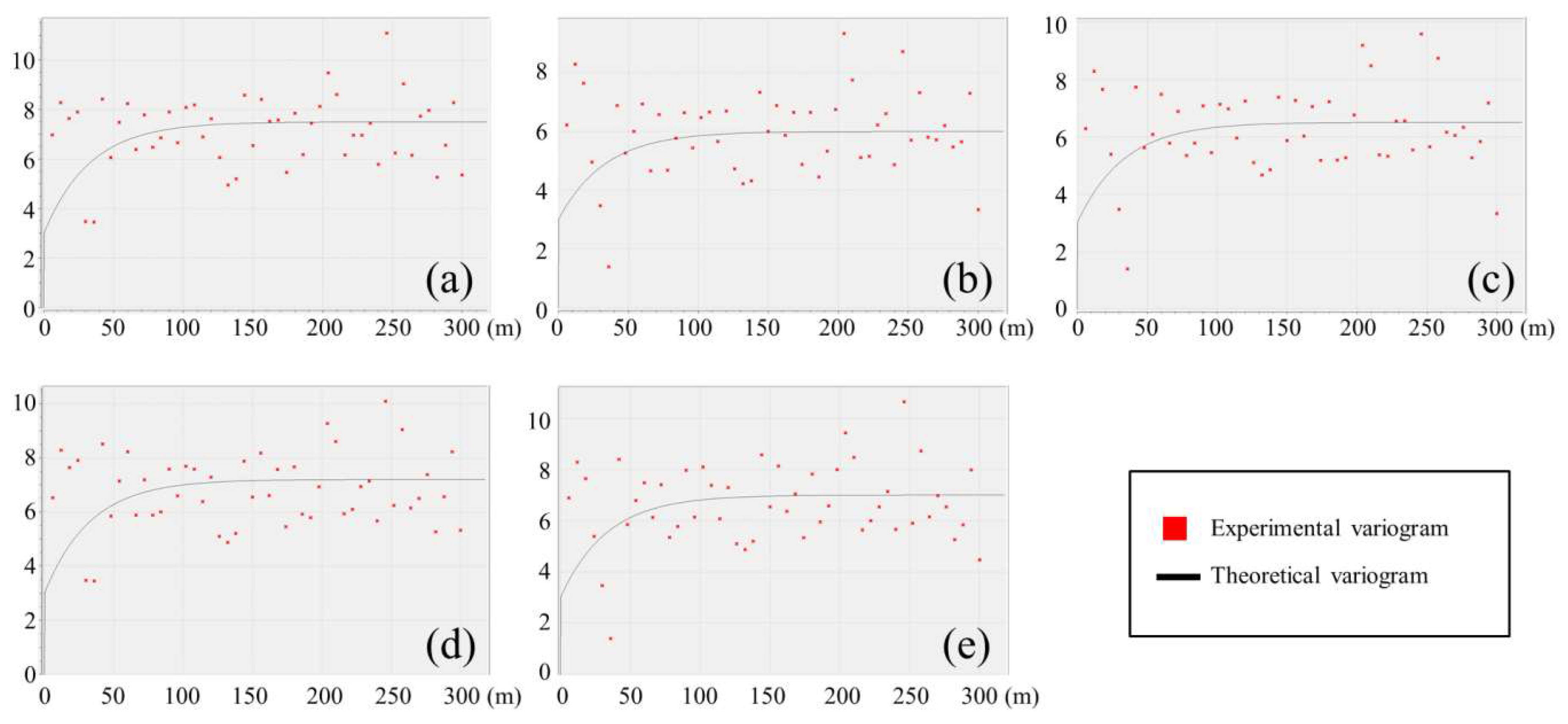
Figure 7.
The kriging results of Au grade estimation using (a) all data or capped data by (b) prob top-cut, (c) perc top-cut, (d) std top-cut, and (e) hot spot top-cut.
Figure 7.
The kriging results of Au grade estimation using (a) all data or capped data by (b) prob top-cut, (c) perc top-cut, (d) std top-cut, and (e) hot spot top-cut.

Figure 8.
Histograms of Au grade estimation using (a) all data or capped data by (b) prob top-cut, (c) perc top-cut, (d) std top-cut, and (e) hot spot top-cut, and (f) histogram of assayed Au grade data.
Figure 8.
Histograms of Au grade estimation using (a) all data or capped data by (b) prob top-cut, (c) perc top-cut, (d) std top-cut, and (e) hot spot top-cut, and (f) histogram of assayed Au grade data.

Figure 9.
Constructed 12 panels which contain boreholes for validating local estimation.

Figure 10.
Validation of the Au grade estimation for each panel using the line-diagram.


Table 1.
Minimum, maximum, average, skewness, and total amount of Au in the vein for each kriging prediction and assay data.
Table 1.
Minimum, maximum, average, skewness, and total amount of Au in the vein for each kriging prediction and assay data.
| Minimum (g/t) | Maximum (g/t) | Average (g/t) | Skewness | Total Amount of Au (t) | ||
|---|---|---|---|---|---|---|
| Ordinary kriging | All data | 6.25 | 11.76 | 8.63 | 0.44 | 15.54 |
| Prob top-cut | 6.37 | 10.39 | 8.30 | 0.14 | 14.95 | |
| Perc top-cut | 6.38 | 10.86 | 8.44 | 0.21 | 15.13 | |
| Std top-cut | 6.29 | 11.15 | 8.55 | 0.26 | 15.40 | |
| Hot spot top-cut | 6.31 | 11.31 | 8.53 | 0.34 | 15.36 | |
| Assayed borehole data | 1.79 | 14.63 | 8.80 | −0.50 | - | |
Table 2.
The average of kriging predictions and borehole data for each panel.
| Panel 01 | Panel 02 | Panel 03 | Panel 04 | Panel 05 | Panel 06 | Panel 07 | Panel 08 | Panel 09 | Panel 10 | Panel 11 | Panel 12 | |
|---|---|---|---|---|---|---|---|---|---|---|---|---|
| A 1 | 7.70 | 9.75 | 10.64 | 9.41 | 8.40 | 7.63 | 8.43 | 9.48 | 7.51 | 8.41 | 8.93 | 9.46 |
| B 2 | 7.59 | 8.76 | 9.79 | 8.65 | 8.35 | 7.70 | 8.42 | 9.12 | 7.51 | 7.94 | 8.31 | 8.56 |
| C 3 | 7.56 | 8.77 | 10.06 | 8.68 | 8.26 | 7.68 | 8.45 | 9.48 | 7.57 | 8.39 | 8.43 | 9.26 |
| D 4 | 7.52 | 9.23 | 10.37 | 8.97 | 8.42 | 7.64 | 8.44 | 9.52 | 7.53 | 8.42 | 8.93 | 9.47 |
| E 5 | 7.73 | 9.47 | 10.52 | 8.97 | 8.34 | 7.65 | 8.44 | 9.48 | 7.54 | 8.38 | 8.43 | 9.26 |
| F 6 | 7.53 | 9.95 | 11.04 | 9.40 | 8.37 | 7.92 | 8.49 | 9.62 | 6.57 | 8.64 | 8.49 | 9.59 |
Ordinary kriging using 1 all data, 2 prob top-cut method, 3 perc top-cut method, 4 std top-cut method, 5 hot spot top-cut method and 6 assayed borehole data.
© 2018 by the authors. Licensee MDPI, Basel, Switzerland. This article is an open access article distributed under the terms and conditions of the Creative Commons Attribution (CC BY) license (http://creativecommons.org/licenses/by/4.0/).
Share and Cite
MDPI and ACS Style
Kim, S.-M.; Choi, Y.; Park, H.-D. New Outlier Top-Cut Method for Mineral Resource Estimation via 3D Hot Spot Analysis of Borehole Data. Minerals 2018, 8, 348. https://doi.org/10.3390/min8080348
AMA Style
Kim S-M, Choi Y, Park H-D. New Outlier Top-Cut Method for Mineral Resource Estimation via 3D Hot Spot Analysis of Borehole Data. Minerals. 2018; 8(8):348. https://doi.org/10.3390/min8080348
Chicago/Turabian StyleKim, Sung-Min, Yosoon Choi, and Hyeong-Dong Park. 2018. "New Outlier Top-Cut Method for Mineral Resource Estimation via 3D Hot Spot Analysis of Borehole Data" Minerals 8, no. 8: 348. https://doi.org/10.3390/min8080348
Note that from the first issue of 2016, this journal uses article numbers instead of page numbers. See further details here.