Orebody Modeling from Non-Parallel Cross Sections with Geometry Constraints


1
School of Resources and Safety Engineering, Central South University, Changsha 410083, China
2
Research Center of Digital Mine, Central South University, Changsha 410083, China
*
Author to whom correspondence should be addressed.
Minerals 2019, 9(4), 229; https://doi.org/10.3390/min9040229
Submission received: 15 March 2019
/
Revised: 29 March 2019
/
Accepted: 10 April 2019
/
Published: 12 April 2019
Abstract
:In this paper, we present an improved approach to the surface reconstruction of orebody from sets of interpreted cross sections that allows for shape control with geometry constraints. The soft and hard constraint rules based on adaptive sampling are proposed. As only the internal and external position relations of sections are calculated, it is unnecessary to estimate the normal directions of sections. Our key contribution is proposing an iterative closest point correction algorithm. It can be used for iterative correction of the distance field based on the constraint rules and the internal and external position relations of the model. We develop a rich variety of geometry constraints to dynamically control the shape trend of orebody for structural geologists. As both of the processes of interpolation and iso-surface extraction are improved, the performance of this method is excellent. Combined with the interactive tools of constraint rules, our approach is shown to be effective on non-trivial sparse sections. We show the reconstruction results with real geological datasets and compare the method with the existing reconstruction methods.
1. Introduction
We focus on the reconstruction of an optimum 3D model from sets of interpreted cross sections in the geological field. In the process of orebody modeling, geological engineers are required to delineate the orebody contours for the region they are interested in on the prospecting section lines based on the borehole sampling data, and reconstruct a 3D orebody model through a series of cross contours.
Because the manually interpreted contours can be used to restrict the boundary of the orebody accurately, explicit modeling methods based on contour splicing are usually the main method of orebody modeling. However, some shortcomings have been found in the explicit modeling method based on contour splicing, such as the inability to update the refined model dynamically, the poor quality of the generated model, and the need for model validity detection. More importantly, most of the explicit modeling methods can only handle the parallel cross sections of the orebody. To solve the above problems, we consider interpolating the contours (parallel or non-parallel) using an implicit function, which can be viewed as an approach of implicit modeling. The reconstructed model is also called as an implicit surface.
For sparse contours, the difficulties in interpolation mainly lie in the need to deal with problems such as model extrapolation, topological relation and branch recombination between sections. Compared with dense data (dense point clouds), sparse data modeling is more complicated due to the greater uncertainty and constraint rules in a particular context. Therefore, it is needed to seek for an efficient section modeling method which has a high degree of automation and facilitates local dynamic adjustment of constraints. Spatial interpolation of contours using implicit functions usually requires estimation of the section normal direction. Although several methods for section normal direction estimation have been proposed, without a priori contour information, its real normal direction is still difficult to be accurately estimated due to the sparsity of the contour. The effect of surface reconstruction methods based on section normal direction estimation relies on continuous iterative correction of the estimated normal direction.
In different application contexts, to satisfy different requirements of the model for local trend and topological relation between contours, it is usually necessary to construct specific constraint rules or perform incremental sampling of sparse data. However, due to uncertainty of the modeling trend, both construction of constraint rules and incremental sampling rely upon the manual dynamic interaction process. For example, for complicated topological relation of multiple contours between sections, it is often difficult to estimate the actual topological connections of the model by relying solely on extrapolation of spatial interpolation, and hence an effective interpolation constraint method has to be available to control the topological relation. Therefore, the modeling process of sparse sections must allow the construction of interactive constraints and achieve dynamic update of the model.
The implicit modeling method is ideal for the construction of interactive constraints and dynamical updating of the model. The method converts the geometric domain constructed on the basis of section data into a distance field via the distance function and expresses the 3D model as a mathematical function, and the reconstructed surface is expressed as a zero level set of the implicit function. However, due to the sparsity of section data, the sparse data interpolation is often poorly interpolated in areas lacking data support, thus it is difficult to create a desired model that conforms to the actual trend of the model.
To effectively recover the original topology between sparse contours, incremental sampling has been performed for the sparse data with large intervals. Based on the adaptively sampled data, the additional constraints are divided into soft and hard constraints according to their reliability. Soft constraints can be corrected based on hard constraints and distance field analysis. According to the principle of minimum point-surface distance of the distance field and the definition of distance in Euclidean space, the iterative closest point correction algorithm is proposed for constructing the optimum signed distance field of incremental sampling constraints. This approach can effectively solve the ambiguity problem of soft constraint distance values between cross sections.
1.1. Related Works
According to the above analysis, we can convert the problem of orebody modeling from interpreted cross sections into surface reconstruction from multiple contours (parallel or non-parallel). Two bodies of works that are close to ours are briefly reviewed, namely, the implicit function, and surface reconstruction from contours.
1.1.1. Implicit Function
We use the implicit function to interpolate the contours. A variety of implicit functions including radial basis functions (RBF) [1,2,3], Hermite RBF [4], Moving Least Squares (MLS) [5], and Multi-Level Partition of Unity (MPU) implicits [6,7] are developed. Among them, RBF is a widely used interpolation method with complete theoretical support. Hoppe et al. [8] constructed a signed distance field function to fit point cloud data by local tangent plane estimation, which provides an idea for defining implicit function using distance field. Example approaches include Dual-RBF method [9], Poisson surface reconstructions [10], smooth signed distance method (SSD) [11] and MPU based methods. Hardy et al. [12] first mentioned the possibility of using Hermite interpolation with MQ-RBF in the multiquadric-biharmonic theoretical analysis, and then the Hermite radial basis functions (HRBF) method with normal constraints was developed gradually. Recently, Macedo et al. [4] derive HRBF implicits from scattered multivariate Hermite data based on the Hermite–Birkhoff interpolation theory with RBFs. Liu et al. [13] proposed a closed-form HRBF implicits method to solve the problem of large-scale point cloud data reconstruction by quasi-interpolation. Recently, several generalized interpolants based on the theory of Hermite–Birkhoff interpolation with RBFs were developed, such as generalized RBF (GRBF) [14] and generalized HRBF (GHRBF) [15]. To handle problems with large numbers of constraint points, efficient methods such as FastRBF [16] and PetRBF [17] are developed based on the RBF method. However, the current implicit functions are often used for surface reconstruction from dense data, particular point clouds, lacking necessary interactive constraint tools.
1.1.2. Surface Reconstruction from Contours
The methods of contours reconstruction can be divided as explicit modeling and implicit modeling. The explicit modeling method [18] based on contours matching has the disadvantages of poor geometric quality of the model and difficulty in dynamic updating. Implicit modeling methods [19,20] based on implicit functions can reconstruct a closed and intersection-free surface and update the model dynamically. Sharma et al. [21] proposed an algorithm for surface reconstruction from unorganized planar cross sections using Hermite mean-value interpolation for triangular meshes. However, the reconstruction effect of this method depends on the quality of meshing. In terms of topological constraints, Zou et al. [22] proposed a topological sampling method for controlling topological relationship of multiple contours, and recently Huang et al. [23] improved this method for reconstructing multi-labeled material interfaces of cross sections. However, the quality of the result reconstructed by this method depends on the post-processing steps, and the constructed model is not an implicit model in nature. For normal estimation, Ijiri et al. [24] improved the previous estimation method [25,26], and proposed a novel contour-based volume image segmentation technique using Bilateral Hermite Radial Basis Functions. However, this method is mainly used for medical imaging. The current contour interpolation algorithms require estimating the normals of contours, while the actual normals of sparse data are unknown and vary with the application background.
2. Overview of the Method
We try to recover an implicit function that exactly interpolates the interpreted contours of the orebody, and reconstructs the implicit surface using iso-surface extraction algorithm.
The contours are usually important information that limit the boundary of orebody based on geological rules, so the exact interpolation methods must be chosen. The RBF-based methods can interpolate sparse data, even when large gaps occur in inputs. Our approach can be seen as a variation of the existing RBF-based methods.
In the process of contours interpolation, we consider the RBF interpolant for implicit surface reconstruction that includes on-surface constraints () and off-surface constraints (). The implicit surface S is defined as , and for short. In R3, based on the idea of distance field, we can obtain N scattered data points with function values of distance to surface by sampling the unknown geological domain.
The goal is to find an implicit function that defines the surface S so that any point p on the reconstructed implicit surface satisfies the following exact interpolation conditions,
where are function values of the domain. The off-surface constraints include two types: Interior constraints () and exterior constraints (). The domain constraints can well control the internal and external position relations of the geological domain and are the most basic constraints to define the geometry shape.
To exactly interpolate the contours using radial basis functions, the contours should be converted into the interpolation conditions in Equation (1). Because the contours cannot be directly added in interpolation equations, the contours should be uniformly sampled and converted into on-surface constraints (the function values are zero). To avoid nontrivial solution, the additional constraints should be constructed.
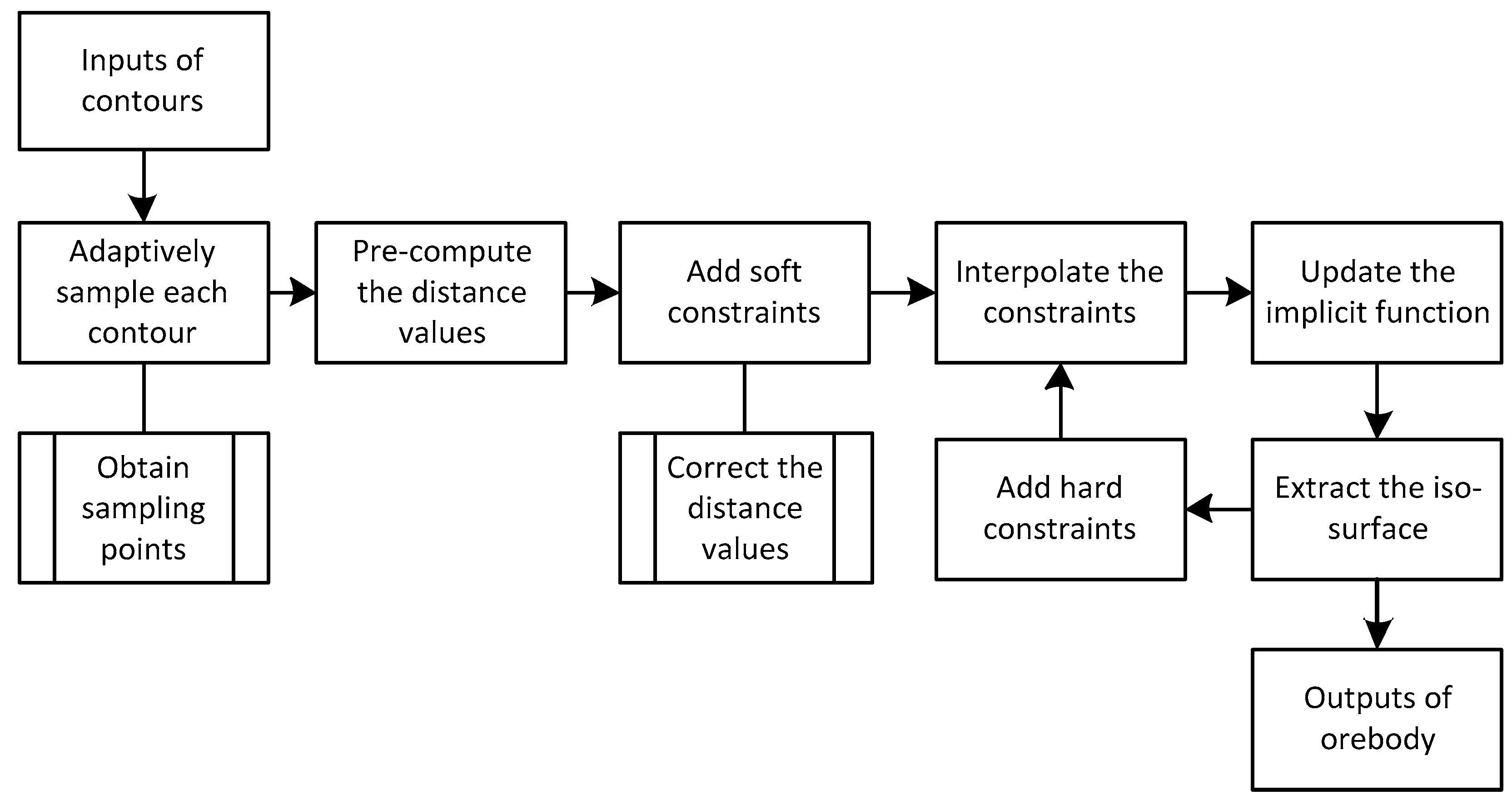
Based on the idea of surface reconstruction using an implicit function, as shown in Figure 1, our approach of contours interpolation is split up into three main steps:
Step 1 (Adaptive sampling): Each contour is located in a 2D plane. Divide the 2D space of each contour into quadtree cells adaptively and obtain the sampling points in the centers of quadtree cells. The sampling points are used to construct interpolation centers.
Step 2 (Additional constraints): Limit the internal and external position of the surface by adding soft constraints and hard constraints. Pre-compute the distance values of the soft constraints.
Step 3 (Distance field correction): Approximate the signed distance field of the implicit surface based on the distance field correction method. And interpolate the interpolation centers and constraints to construct a signed distance field using an implicit function.
Finally, the implicit 3D orebody models can be recovered using the fast iso-surface extraction method. We shall detail each step in the following sections. In the Results section, the numerical results and the comparisons of the existing methods are undertaken. In the Discussion and conclusion section, we discuss the limitations and extensions of this method in the last section.
3. Contours Interpolation
3.1. Implicit Function
The goal is to find an implicit function that defines the surface S so that any point p on the reconstructed implicit surface satisfies the exact interpolation conditions in Equation (1).
According to the interpolant of the Beppo-Levi space, a measure of the energy or “smoothness” of function s(x) can be defined as
And the smoothest interpolant of RBFs has the form
where are the coefficients to be determined, are the interpolation centers and the usual radial basis function can be viewed as a function of . When conditionally positive definite functions are used, it’s often required to construct low-order polynomials to ensure that the function converges. Assuming the polynomial part has the form , the smoothest interpolant requires to satisfy the orthogonality or side conditions:
There are many common radial basis functions for different applications, as shown in Table 1. For three-dimensional surface modeling, the biharmonic and triharmonic splines are recommended.
These side conditions along with the interpolation conditions lead to a linear system, and the matrix form can be written as
where , and the unknown coefficients and can be determined by solving the linear system . To accelerate the speed of surface reconstruction, the fast evaluation and fast solution methods are recommended to implement.
3.2. Adaptive Sampling
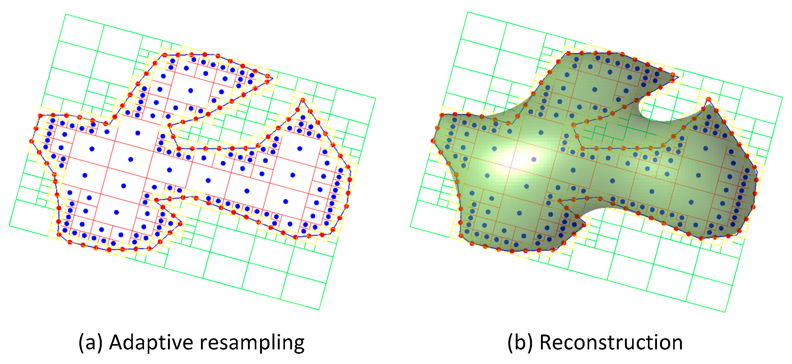
As the regular grid sampling consumes much memory and results in oversampling, the adaptive sampling method is adopted. During sampling, the quadtree structure is used for space division of the closed curve, and the sampling results are used for construction of interpolation constraints.
The sampling parameters, boundary subdivision levels, internal subdivision levels and external subdivision levels are defined to control the boundary cells (intersect the contour), internal cells (inside the contour) and external cells (outside the contour). The 3D coordinates can be converted into 2D coordinates by taking the average plane where a contour is located as the projection plane. Each cross section is partitioned by section contours into inside/outside regions. Traverse each contour, 2D adaptive sampling is performed for the closed curve through a quadtree division algorithm in the bounding box of this contour. A simple reconstruction example of a contour is shown in Figure 2. In iterations of space division, the cells of quadtree will be continually divided if the corresponding cell depth does not exceed the specified subdivision level.
As the sampling process is performed separately for each contour, there may be some intersecting sampling cells in the overlapping domain. To avoid repetitive interpolation constraints, a process for filtering repetitive cells will be executed at the end of sampling. Fast spatial indexing algorithms, such as Kd-tree [27], are used to filter repetitive sampling cells whose center spacing is within a certain tolerance range, thus avoiding repetitive constraints at the end of later construction of interpolation constraints. Next, during construction of additional constraints, the distance values of these sampling points will be computed.
3.3. Additional Constraints
To interpolate the contour, the sampling points should be converted into interpolation constraints, and these additional constraints can be categorized into soft and hard constraints. A soft constraint is an approximate constraint that needs to be corrected later, while a hard constraint is a deterministic or manually specified constraint that must be exactly interpolated. For example, the boundary constraints on the contours are hard constraints.
3.3.1. Soft Constraints
To distinguish between internal and external relationships of the model, the constructed incremental sampling method can be used to change the connection trend and topology of the model. The off-surface constraints constructed based on the adaptive sampling cell can be used to define soft constraints.
By calculating the closest distance from the cell center to the contour, it is possible to simply construct internal and external off-surface constraints with the center of the sampling cell as the constraint points. We directly calculate the function values of off-surface constraints based on the distance field instead of estimating the section normal direction (to construct an off-surface constraint by offsetting a certain length from the normal direction). The signed distance field implicit function of multiple contours in the same cross section can be defined as
where is a two-dimensional sampling point at in each cross section, and is the nearest distance from to the closest point on the all contours in the same cross section. The distance values will be approximately corrected as the nearest distance to all contours in three-dimensional space.
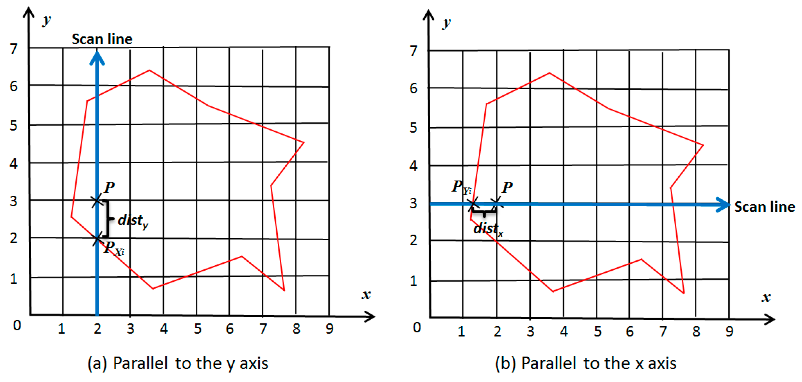
The higher the precision requirement of the model reconstruction, the higher the sampling cell density and the more time it will take to calculate the distance value for each point. To improve the distance field calculation speed, fast space detection algorithms such as oriented bounding box (OBB) tree collision detection method [28] can be adopted to avoid massive invalid intersection operations. Refer to relevant literature for details. To further improve the distance field calculation speed, the method to achieve distance field calculation via the expansion of non-Euclidean distance transformation by means of scanning proposed by Bi et al. [25] can be easily realized, for regular sampling is an exception of adaptive sampling. As shown in Figure 3, the basic idea of this method is to replace with the minimum x-direction boundary distance and y-direction boundary distance, and use the scan lines parallel to x axis and y axis to calculate the minimum x-direction and y-direction boundary distances of all points on the scan lines. As the distance transferring effect is satisfactory, only a few simple intersection calculations are required for each scan line. This method takes full advantage of distance correlation between sampling cells, which can effectively reduce the time and space complexity of the algorithm.
3.3.2. Hard Constraints
To guide the interpolation trend in sparse regions, the user can steer the method by adding hard constraints in interactive ways. According to the prior knowledge, it is convenient for the user to dynamically edit and update the models step by step.
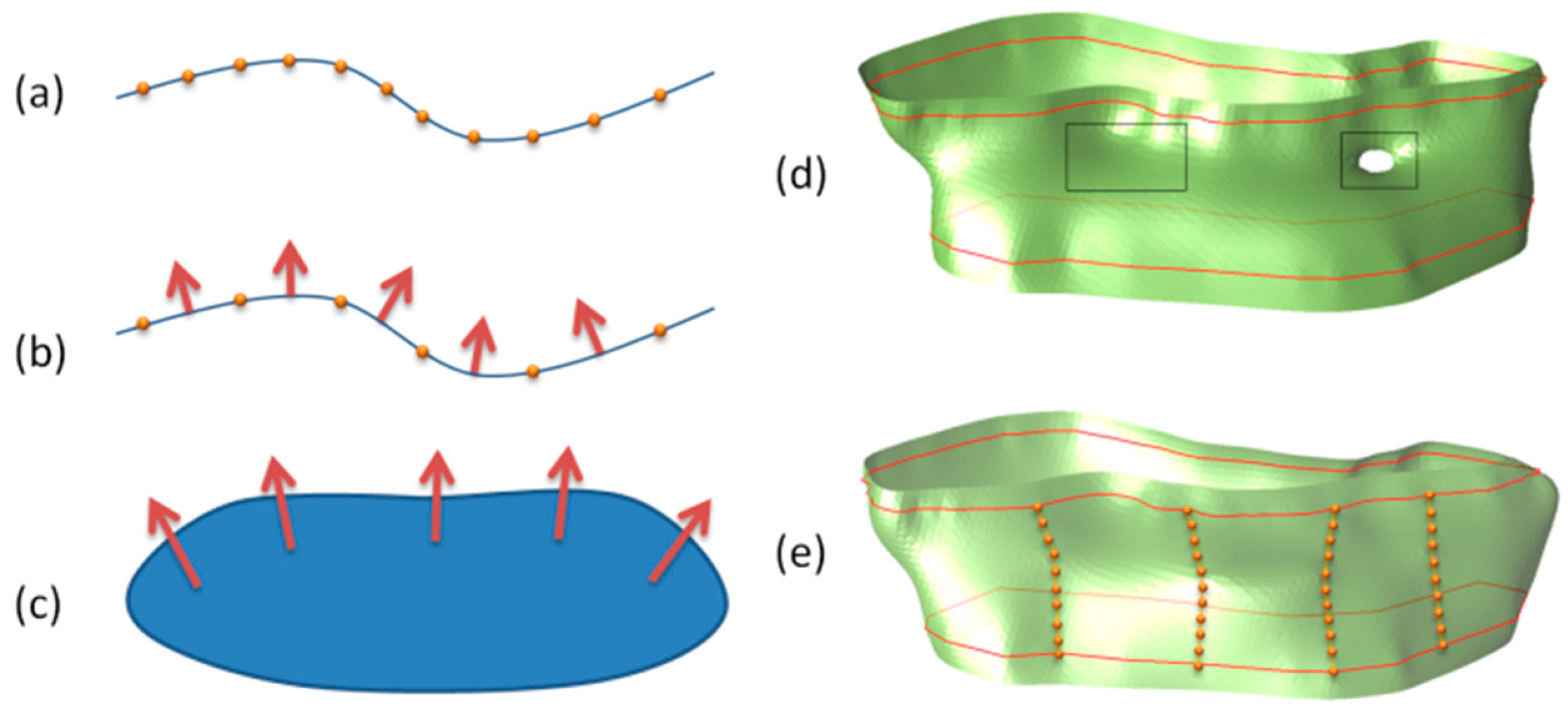
Constraint point: A constraint point is the control point added by user interactions. It is used to characterize the model boundary and the surface shape. The local trend of sparse and non-uniform data as well as the continuity of model can be changed by adding constraint points, as shown in Figure 4. And the reconstructed 3D model conforms to the limitations of constrain points.
Constraint line: Adding constraint lines is a more effective choice when it is required to control the larger trends of extrapolation. A constraint line can be transformed into points with normals. The normal directions can be estimated by the average plane where the constraint line is located. The positive direction (pointing to the outside of the model) of the normal direction is determined in combination with the internal and external relationships of the model. When the normal directions are determined, we can interpolate the points with normals by offsetting points along the directions of normals using radial basis functions [26]. Some of our examples show that it is useful to add constraint lines, especially for sparse contours.
Trend surface: As mentioned above, it is not necessary to estimate the normal directions of the contour. However, in case of a priori direction information, such as a manually specified trend surface, the trend surface can be used to solve the 3D space vector field to characterize the gradient transformation of the interpolation space. The estimation of the contour normal direction can be calculated according to the interpolation result of the vector field, while the accurate estimation of the normal direction of the model boundary can well control the geometrical morphology of the implicit model.
3.4. Distance Field Correction
To avoid repeated, abnormal and ambiguous distance function values, these values should be verified prior to construction of the corrected distance field.
3.4.1. Distance Estimation
The principle of our distance field correction method is mainly based on the definition of Euclidean distance. In the distance filed, the signed implicit function shall satisfy the principle of the minimum point-surface distance and the definition of distance in Euclidean space. According to the triangular inequality condition in the three conditions that must be met according to the definition of Euclidean distance, the definition of the signed distance field is combined:
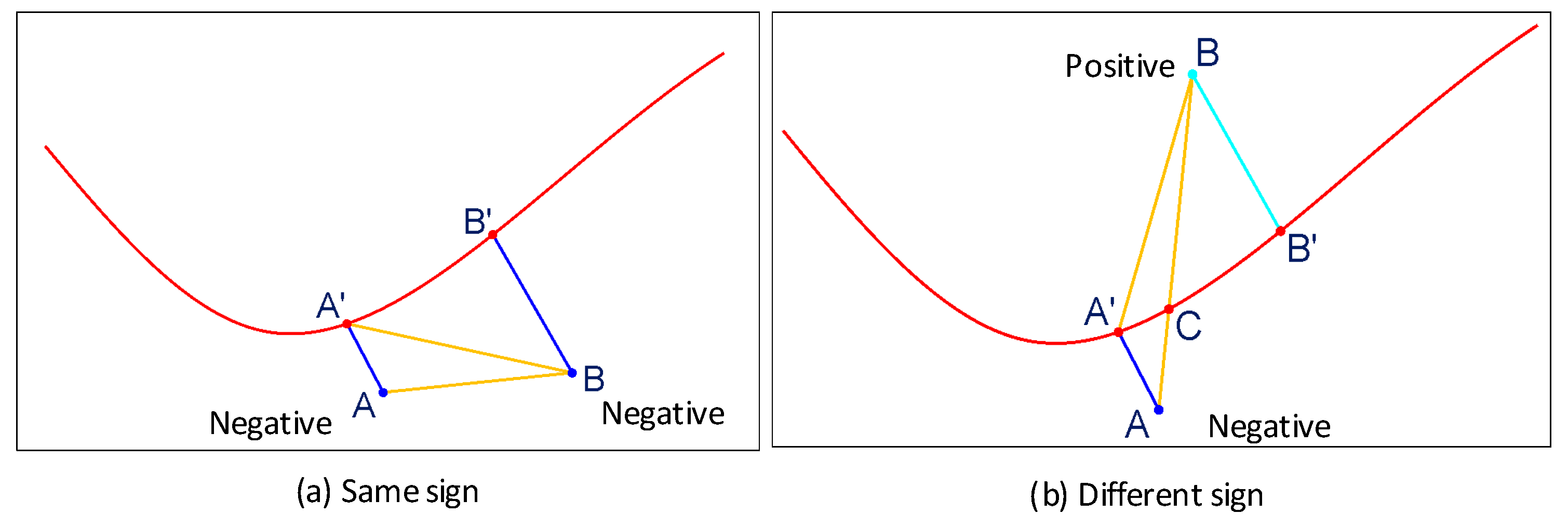
where point A and point B are arbitrary interpolation center points in the geological domain, while point and point are respectively the closest points from point A and point B to the surface, where . The signs of distance values are defined as follow: Points inside the model are negative and points outside the model are positive. According to the sign difference between and , as shown in Figure 5, it can be divided into two cases:
In case and share the same signs,
In case signs of and are opposite (one positive and the other negative),
Therefore, for each off-surface constraint, the formula shall be satisfied, otherwise the distance value shall be corrected. During distance field correction, both soft and hard constraints shall be considered. The distance field correction only iteratively corrects the distance values of soft constraints, while hard constraints are only used for distance correction calculations (without involving in distance correction).
3.4.2. ICPC
Based on the analysis of distance estimation, we propose an iterative closest point correction (ICPC) algorithm to construct a distance field that is more suitable for the domain distribution trend, so as to solve the ambiguity problem of estimated distance values of soft constraints between cross sections.
The basic idea of ICPC is to verify the estimated 2D distance value (non-minimum point-surface distance) in a soft constraint based on a series of constraint points with validated distance values (including hard constraints and corrected soft constraints) in 3D. Though every two points should satisfy Equations (8) and (9), to simplify the problem, we only consider the distance correction problem iteratively in the neighborhood of a point. In case and share the same signs, if at point A, the distance value of point A should be corrected as . In case signs of and are opposite, if , the distance value of point A should be corrected as .
For a signed distance field, in order not to affect the boundary, the internal and external constraint points will be separately addressed. Taking the case of the same sign as an example, the specific process of the iterative closest point correction algorithm is described in detail as follows:
Step 1: Sort the soft constraints. As the iterative process is a process of gradually reducing the distance values. To avoid a large number of repeated comparisons, each soft constraint point will be sorted from the smallest to the largest according to the distance value, the set of which is s;
Step 2: Initialize . Construct a currently minimum correction distance value . As the initial value for distance verification, its initial value is set to be zero;
Step 3: Find a comparison point. Traverse the set s, select a soft constraint point from the set s of values that are not smaller than , and use the kd-tree spatial indexing algorithm to seek for the point that is closest to , as the reference point for distance comparison;
Step 4: Verify and correct the distance value. Verify according to the distance judgment formula. In case of , the distance value of point A shall satisfy , without changing the sign of its distance value (internal and external properties);
Step 5: Update and repeat the iteration. If the distance value of is corrected, re-sort the set s. Update according to the latest distance value of . Return to Step 3 and end the process until the iterative process converges.
Because the distance value of a soft constraint may be corrected many times, the sorting of distance values reduces the comparisons of iterative process. Since the correction of the distance value is a process of gradually reducing the distance value, the iterative process can maintain a convergence trend. In the worst case, although unlikely, all the other points of a soft constraint point should be corrected. Our experiments showed that the iterative process converges in .
4. Fast Reconstruction
The computational complexity of the general interpolation algorithm depends on the number of interpolation constraints and grid resolution for surface reconstruction. To accelerate the process of dynamical modeling, both of the solution of the linear system and the surface reconstruction must be improved.
The interpolation equation is a large-scale symmetric dense linear system of equations. The spatial complexity and time complexity solved with conventional direct methods such as lower–upper (LU) decomposition and singular-value decomposition (SVD) decomposition are difficult to adapt to the spatial interpolation of large-scale scattered data. The adopted fast multipole method (FMM) which is introduced into radial basis function interpolation problems by Carr et al. [26] not only decreases the solved spatial and time complexity but also reduces the ill-conditioned problem of a large-scale dense system of equations through approximate solution. The essence of FMM is to divide the interpolation data into near-field data and far-field data according to the distance from the center of the interpolation . The near-field data is solved with the direct method, while the far-field data is solved with the approximate method within a certain error range. Therefore, the speed of interpolation calculations can greatly be improved [29,30].
In terms of reconstruction of implicit models, the conventional iso-surface extraction algorithm (e.g., Marching Cubes) requires function evaluation of the sampling points on the regular grids. To ensure fast dynamic update of the implicit model, in addition to fast solution of interpolation equations for the implicit model, fast evaluation of interpolation points for the implicit model should also be realized. By constructing the initial voxel seed points and using certain voxel growth rules [31] to track the surface reconstruction process, we can avoid the radial basis functions from evaluating the function values on all voxel grid points and thus speed up the process of surface reconstruction.
5. Results
5.1. Examples
Based on the above algorithms such as spatial interpolation and iso-surface extraction, we implemented the method of fast surface reconstruction of cross sections using Microsoft Visual Studio 2012 (C++ language). We tested the method on several real geological datasets for orebody modeling. To compare the other methods, we also tested some real medical datasets. The datasets were obtained from the Digital Mine National Lab, Liu et al. [18] and Zou et al. [22].
The method utilizes several parameters, some offering the sampling accuracy of the contours, and others providing the reconstruction accuracy of the models. The following set of parameters, sampling interval in cross sections (), boundary subdivision level (), internal subdivision level () and size of resolution () should be determined. We use the following values for all our real-life examples: , , and initially, where is the diagonal of the bounding box of the contours. In many cases, we don’t need to adjust the values of and . Similar to other methods, the desired reconstruction accuracy and smoothness of the models can be obtained by adjusting the values of and .
We demonstrate the robustness of our approach about the precision of intersections between two contours in Figure 6. The method of Liu et al. [18] produces undesired artifacts and is not consistent with the contours (Figure 6c). The method can exactly interpolate the contours (Figure 6d) in spite of the intersection errors between two contours (Figure 6b). Moreover, the constraint lines (Figure 6e) can be used to control the extrapolation of the shape and dynamically update the model.
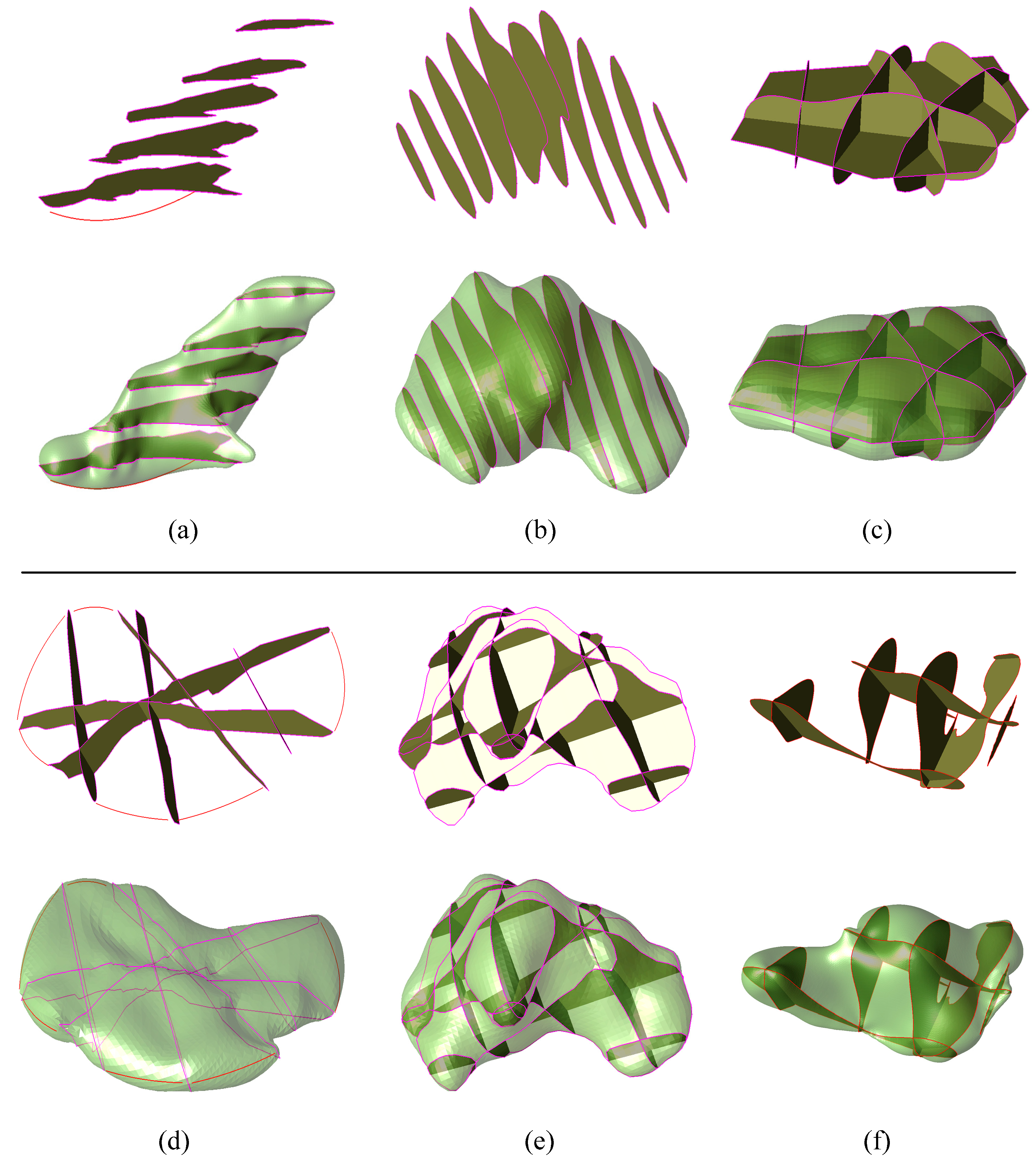
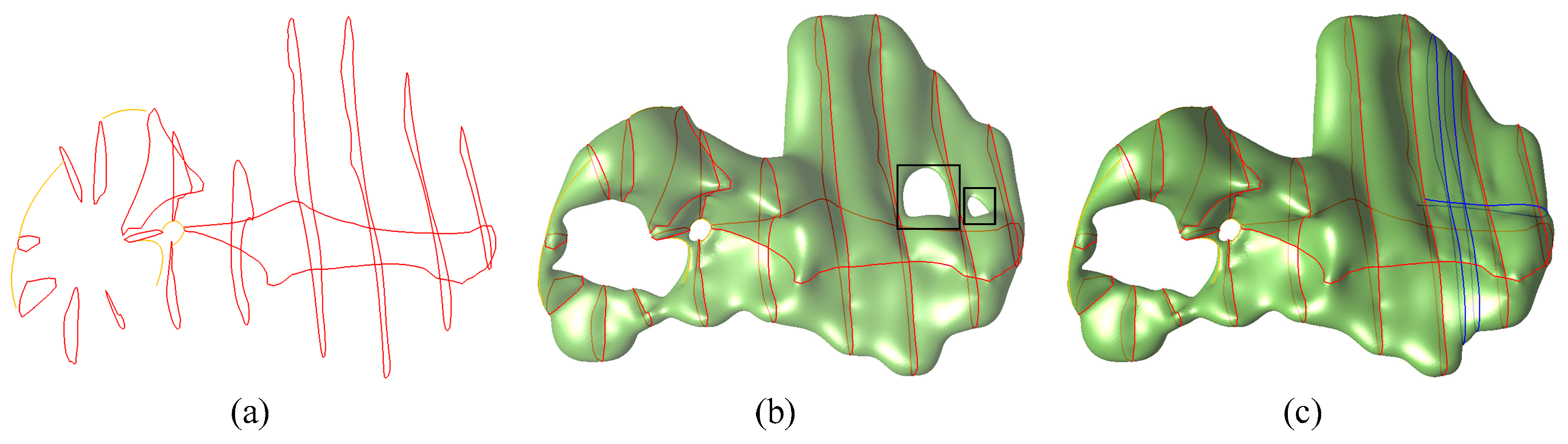
To test the universality of the algorithm, several types of data sets were constructed, as shown in Figure 7. The results suggest that for dense parallel sections, the results of sampling the contours can contribute to well reconstruction of the original model without adding geometry constraints. For sparse cross-sections, to control the extrapolation of the shape, hard constraints (in Figure 7a,d) should be interactively added to limit the model boundary. For non-parallel cross-sections, on the one hand, contours play a better role in restricting the internal and external positions of the model, which can better recover the original model; on the other hand, sampling between intersecting contours is likely to cause ambiguous constraints, resulting in anomalies such as distortions and dents for the reconstructed model. The process of distance field correction is used to avoid ambiguous constraints.
Taking an input of non-parallel cross sections as an example, several representative algorithms were selected for comparison, as shown in Figure 8. Compared with the implicit modeling method, explicit modeling (Figure 8b) requires more human interaction processes, and the method of Zou et al. [22] is featured with the disadvantages of poor model quality and dependence on post-processing. In case of no correction of the distance field, it is likely to produce deformations such as depressions and distortions. The reconstruction effects before (Figure 8d) and after (Figure 8e) distance field correction were compared in Figure 8. Due to the uncertainty of sparse data modeling, it is often required to change the local trend of the model by adding local constraints in actual modeling. However, compared with the method with hard constraints, the method without hard constraints (Figure 8e) cannot change the actual topological relation or extension trend of the model by constructing the model constraint relation.
5.2. Performance
The performance of the improved method mainly depends on the number of constraints and the size of resolution. We implemented our algorithm in C++ and tested on a Windows 64-bit PC with 3.20 GHz Intel(R) Core(TM) i5-3470 and 4GB RAM. Table 2 reports the timings of the interpolation and reconstruction stages of our algorithm on these examples. The relative geometric error is defined as the root mean square error (RMSE) [32] relative to the diagonal of the bounding box of real-life object.
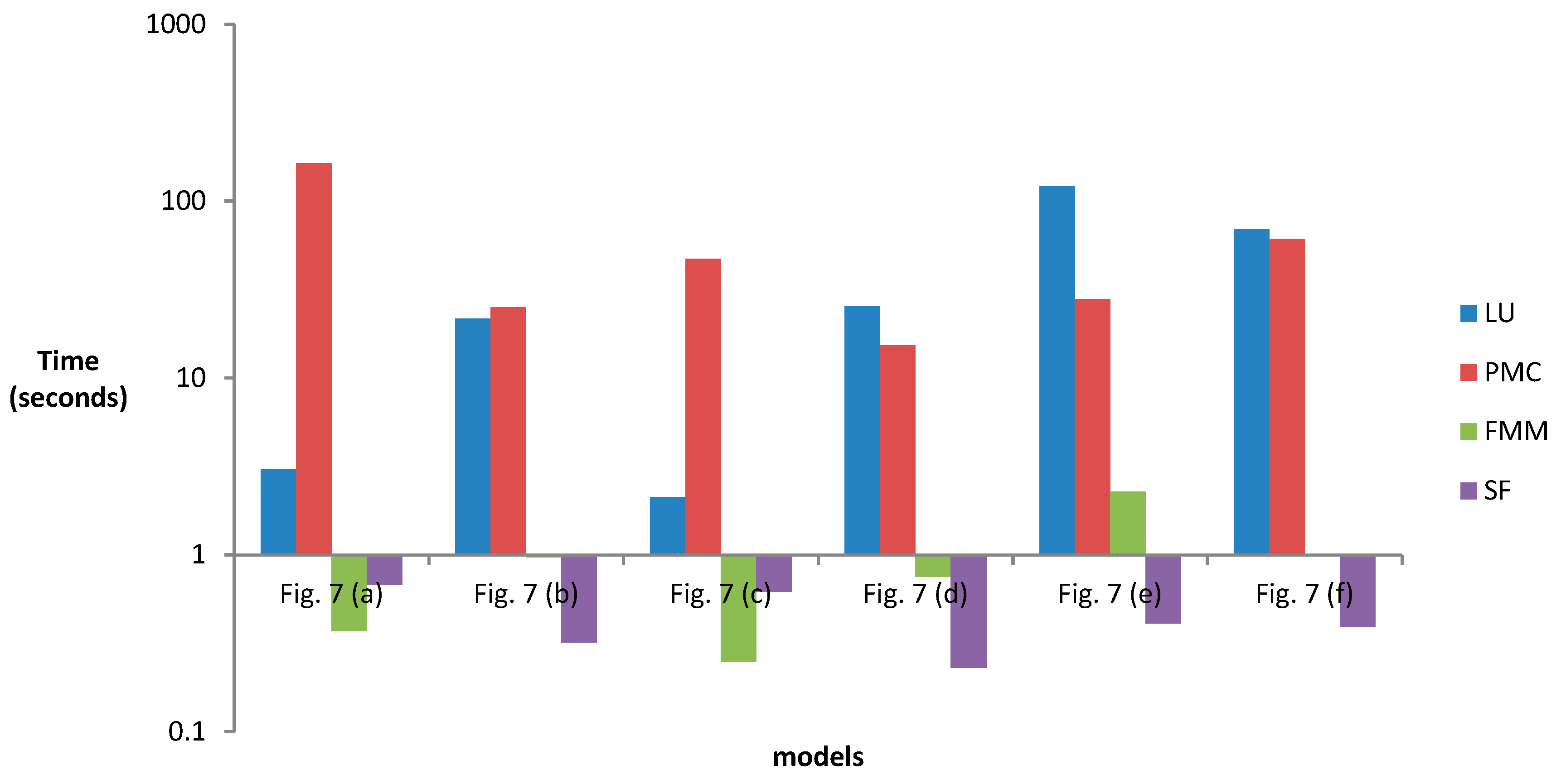
To test the performance of fast reconstruction using the improved method, we compared the running efficiency of multiple data sets before and after improvement, as shown in Figure 9 (related to Table 2). Compared with the traditional direct method (LU decomposition) to solve the linear systems, Table 2 shows that the FMM algorithm we use has faster solution efficiency. Similarly, the surface following (SF) algorithm we use has faster reconstruction efficiency than the traditional Marching Cube (MC) and parallel Marching Cube (PMC) extraction method. Moreover, as the size of the solution equations larger or the reconstruction resolution decreases, the performance advantage of the improved algorithm is more obvious.
6. Discussion and Conclusions
In this paper, we propose an improved cross-section modeling method that allows the interactive addition of geometric constraints and the dynamic update of the mesh in the process of orebody modeling. Our main contribution is based on the idea of incremental sampling and potential field iterative correction. An iterative closest point correction algorithm is proposed. It can be used for iterative correction of the distance field based on constraints and internal and external relations of the model. Moreover, the FMM and surface tracking methods are adopted to improve the interpolation and reconstruction efficiency of the method. It can perform efficient interpolation and surface reconstruction for large-scale constraints, thus enhancing the efficiency of surface reconstruction after incremental sampling of sparse data of orebody.
Orebody modeling is a process that is gradually refined as the sampling progresses. When the sampling data changes locally, it is necessary to re-interpret the contours of the orebody, delineate sections and splice parallel or non-parallel cross sections, which are difficult to adapt to the requirements of resource reserves estimation and dynamic update of orebody models in the stage of production and exploration. According to our approach, the structural geologists can append variety of constraints into the raw data to re-solve the implicit function of the orebody and hence dynamically reconstruct the model. As the RBF interpolant is an exact interpolation method, the soft and hard constraints can exactly limit the boundary of the orebody. By adding specific hard constraints, the reconstructed models of the orebody are more consistent with the geological features and mineralization trends.
6.1. Limitations
The objective of this paper is to obtain a more automated, efficient and robust orebody modeling approach from cross sections. However, there are still some limitations to our work that need to be improved.
One of them is the lack of an effective constraint method for topological relation. The tangent plane where the section is located can help to determine the internal and external relations of the model through the contour, but the spacing and the gap between the sections are completely determined by extrapolating the interpolation. For sparse and non-uniform section data, it is often difficult to effectively restore the complex topological relation of multiple contours between sparse sections by relying solely on extrapolation of spatial interpolation. Zou et al. [22] explored the topological relation between contours through topological sampling. It is a constructive method, but with a disadvantage that the model quality depends on the post-processing smoothing process. Although it is possible to change the local topological relation of the model by constructing additional constraints, it relies on more human interaction processes. Therefore, it is necessary to construct additional trend constraint rules to control the topological relation and extrapolation trend of the model.
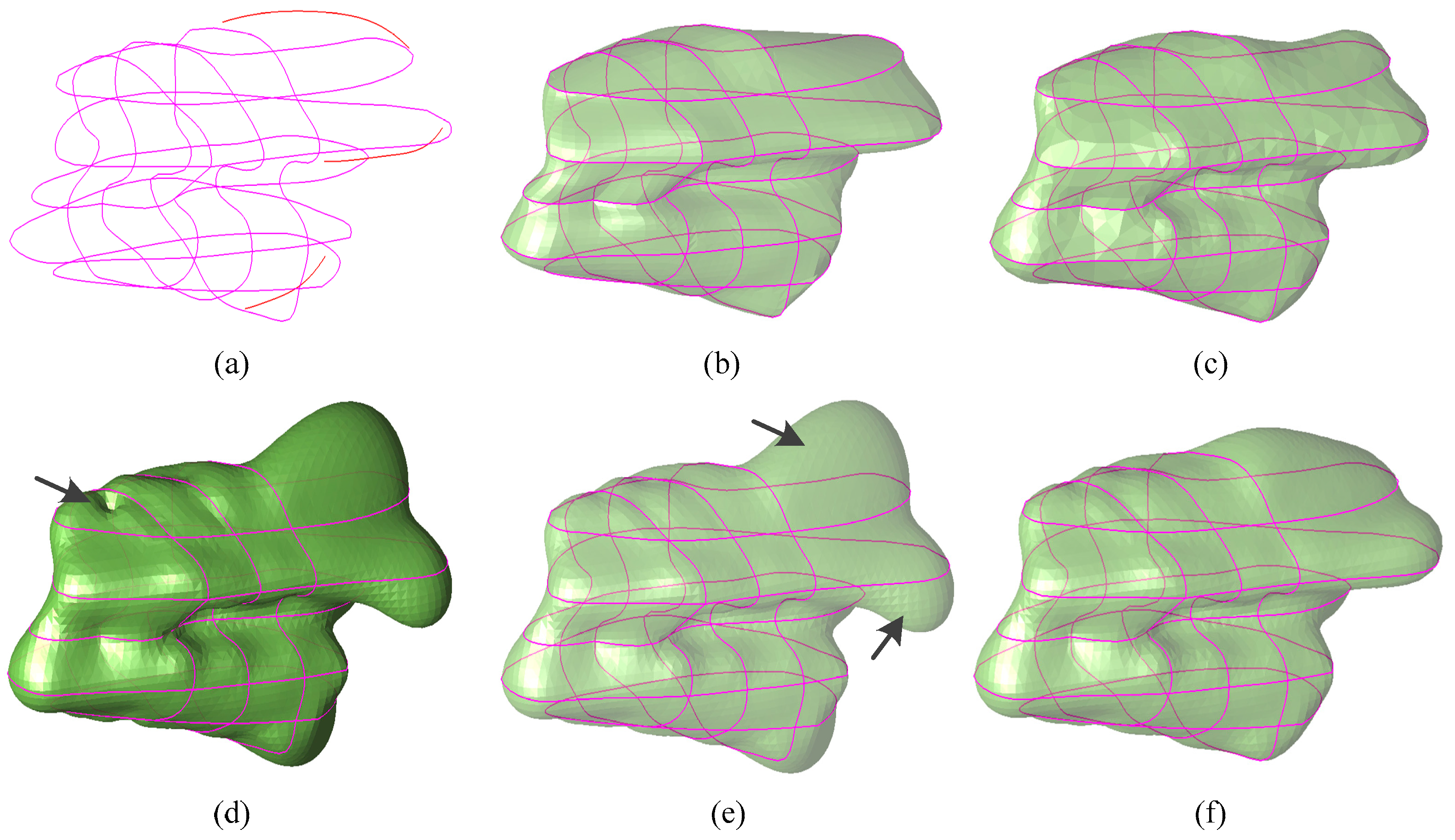
Another limitation to this approach is that, for sparse and thin sections with large intervals, the reconstructions are likely to produce many discontinuities. This type of data is a notoriously ill-posed problem and hence requires much extrapolation; there is still much work to be done. As shown in Figure 10b, the results of sparse section modeling are often not ideal without adding constraint rules, which is also a common problem in sparse data modeling [22]. Additional constraint lines (blue lines in Figure 10c can help to solve this problem, but it requires more human interactions and iterative modeling processes. Another feasible approach is to perform incremental sampling according to the model trend to construct well-connected sampling data between sections, which is also an extension of this paper.
6.2. Extensions
To enhance the robustness and adaptability of this method, it is necessary to satisfy the requirement of the algorithm for the inputs. Our approach requires that the input data should be a closed curve on a set of tangent planes, which is determined by the sampling method adopted in this paper. However, this limitation can be avoided by constructing hard constraints. In this paper, the algorithm of contour reconstruction is introduced by taking adaptive sampling of cross-sections as an example. By studying the internal and external relations between the contours, this method is also applicable to the surface reconstruction from non-planar contours in 3D. The results of surface reconstruction using this method largely depend on the effect of incremental sampling. By constructing different sampling methods, 3D reconstruction of complex models with special structures such as flat and distorted ones can be performed. Based on the idea of incremental sampling and potential field iterative correction, this method can be well applied to surface reconstruction of sparsely sampled data with specific constraints.
Another important extension is to perform incremental sampling of the geometric field based on the contour information in accordance with possibilities within and without the model. Considering the internal and external relations of the model simply by the tangent plane where the contour is located ignores the influence on the model trend between contours. To make full use of the model trend between contours and the constraint rules in the context of specific applications, an incremental sampling method involving constraint information shall be studied. Meanwhile, we are also studying generalized constraint rules [33] based on the generalized interpolation methods, and using the iterative nearest point correction algorithm to correct the distance field on the basis of different constraint rules.
Author Contributions
D.-Y.Z. and L.-G.W. conceived, designed, and performed the experiments; M.-T.J., L.B. and J.Z. analyzed the data and revised the methodology; D.-Y.Z. wrote the paper; all authors discussed the results and revised the paper.
Funding
This work was financially supported by the National Natural Science Foundation of China (41572317), the National Key R&D Program of China (2017YFC0602905) and the Fundamental Research Funds for the Central Universities of Central South University (2017zzts183). We also thank the reviewers for their comments and suggestions to improve the quality of the paper.
Acknowledgments
Thanks to the public datasets used in this research.
Conflicts of Interest
The authors declare no conflict of interest. The funders had no role in the design of the study; in the collection, analyses, or interpretation of data; in the writing of the manuscript, and in the decision to publish the results.
References
- Sarra, S.A. Regularized symmetric positive definite matrix factorizations for linear systems arising from RBF interpolation and differentiation. Eng. Anal. Bound. Elem. 2014, 44, 76–86. [Google Scholar] [CrossRef] [Green Version]
- Cuomo, S.; Galletti, A.; Giunta, G.; Marcellino, L. Reconstruction of implicit curves and surfaces via RBF interpolation. Appl. Numer. Math. 2017, 116, 157–171. [Google Scholar] [CrossRef]
- Skala, V. RBF Interpolation with CSRBF of Large Data Sets. Procedia Comput. Sci. 2017, 108, 2433–2437. [Google Scholar] [CrossRef]
- Macêdo, I.; Gois, J.P.; Velho, L. Hermite Interpolation of Implicit Surfaces with Radial Basis Functions. In Proceedings of the 2009 XXII Brazilian Symposium on Computer Graphics and Image Processing, Rio de Janiero, Brazil, 11–15 October 2009. [Google Scholar]
- Shen, C.; O’Brien, J.F.; Shewchuk, J.R. Interpolating and approximating implicit surfaces from polygon soup. In Proceedings of the SIGGRAPH ’05, Los Angeles, CA, USA, 31 July–4 August 2005; p. 181. [Google Scholar]
- Ohtake, Y.; Belyaev, A.; Alexa, M.; Turk, G.; Seidel, H.-P. Multi-level partition of unity implicits. ACM Trans. Graph. 2003, 22, 463. [Google Scholar] [CrossRef] [Green Version]
- Chen, Y.-L.; Lai, S.-H.; Lee, T.-Y. Generalized MPU Implicits Using Belief Propagation. In Proceedings of the Sixth International Conference on 3-D Digital Imaging and Modeling (3DIM 2007), Montreal, QC, Canada, 21–23 August 2007; Volume 49, pp. 400–407. [Google Scholar]
- Hoppe, H.; Derose, T.; Duchamp, T.; McDonald, J.; Stuetzle, W. Surface reconstruction from unorganized points. ACM SIGGRAPH Comput. Graph. 1992, 26, 71–78. [Google Scholar] [CrossRef] [Green Version]
- Lin, Y.; Chen, C.; Song, M.; Liu, Z. Dual-RBF based surface reconstruction. Vis. Comput. 2009, 25, 599–607. [Google Scholar] [CrossRef]
- Kazhdan, M.; Hoppe, H. Screened poisson surface reconstruction. ACM Trans. Graph. 2013, 32, 1–13. [Google Scholar] [CrossRef] [Green Version]
- Calakli, F.; Taubin, G. SSD: Smooth Signed Distance Surface Reconstruction. Comput. Graph. 2011, 30, 1993–2002. [Google Scholar] [CrossRef] [Green Version]
- Hardy, R.L.; Nelson, S.A. A multiquadric-biharmonic representation and approximation of disturbing potential. Geophys. Res. Lett. 1986, 13, 18–21. [Google Scholar] [CrossRef]
- Liu, S.; Wang, C.C.L.; Brunnett, G.; Wang, J. A closed-form formulation of HRBF-based surface reconstruction by approximate solution. Comput. Des. 2016, 78, 147–157. [Google Scholar] [CrossRef]
- Hillier, M.J.; Schetselaar, E.M.; De Kemp, E.A.; Perron, G. Three-Dimensional Modelling of Geological Surfaces Using Generalized Interpolation with Radial Basis Functions. Math. Geosci. 2014, 46, 931–953. [Google Scholar] [CrossRef]
- Gois, J.P.; Trevisan, D.F.; Batagelo, H.C.; Macêdo, I. Generalized Hermitian Radial Basis Functions Implicits from polygonal mesh constraints. Vis. Comput. 2013, 29, 651–661. [Google Scholar] [CrossRef]
- Torres, C.E.; Barba, L.A. Fast radial basis function interpolation with Gaussians by localization and iteration. J. Comput. Phys. 2009, 228, 4976–4999. [Google Scholar] [CrossRef]
- Yokota, R.; Barba, L.A.; Knepley, M.G. PetRBF—A parallel O(N) algorithm for radial basis function interpolation with Gaussians. Comput. Methods Appl. Mech. Eng. 2010, 199, 1793–1804. [Google Scholar] [CrossRef]
- Liu, L.; Bajaj, C.; Deasy, J.O.; Low, D.A.; Ju, T. Surface Reconstruction from Non-Parallel Curve Networks, Computer Graphics Forum; Wiley Online Library: Hoboken, NJ, USA, 2008; pp. 155–163. [Google Scholar]
- Akkouche, S.; Galin, E. Implicit surface reconstruction from contours. Vis. Comput. 2004, 20, 392–401. [Google Scholar] [CrossRef]
- Ju, T.; Warren, J.; Carson, J.; Eichele, G.; Thaller, C.; Chiu, W.; Bello, M.; Kakadiaris, I. Building 3D surface networks from 2D curve networks with application to anatomical modeling. Vis. Comput. 2005, 21, 764–773. [Google Scholar] [CrossRef]
- Sharma, O.; Agarwal, N. 3d surface reconstruction from unorganized sparse cross sections. In Proceedings of the Graphics Interface, Victoria, BC, Canada, 1–3 June 2016; pp. 33–40. [Google Scholar]
- Zou, M.; Holloway, M.; Carr, N.; Ju, T. Topology-constrained surface reconstruction from cross-sections. ACM Trans. Graph. 2015, 34, 128. [Google Scholar] [CrossRef]
- Huang, Z.; Zou, M.; Carr, N.; Ju, T. Topology-controlled reconstruction of multi-labelled domains from cross-sections. ACM Trans. Graph. 2017, 36, 1–12. [Google Scholar] [CrossRef]
- Yoshizawa, S.; Sato, Y.; Ijiri, T.; Ito, M.; Yokota, H. Bilateral Hermite Radial Basis Functions for Contour-based Volume Segmentation. Comput. Graph. 2013, 32, 123–132. [Google Scholar]
- Bi, L.; Liu, X.; Chen, X.; Zhu, Z. An automatic 3d modeling method based on orebody contours. Geomat. Inf. Sci. Wuhan Univ. 2016, 41, 1359–1365. [Google Scholar]
- Carr, J.C.; Beatson, R.K.; Cherrie, J.B.; Mitchell, T.J.; Fright, W.R.; McCallum, B.C.; Evans, T.R. Reconstruction and representation of 3D objects with radial basis functions. In Proceedings of the 28th Annual Conference on Computer Graphics and Interactive Techniques, Los Angeles, CA, USA, 12–17 August 2001; ACM Press: New York, NY, USA, 2001; pp. 67–76. [Google Scholar] [Green Version]
- Nuchter, A.; Lingemann, K.; Hertzberg, J. Cached kd tree search for icp algorithms. In Proceedings of the 6th International Conference on 3-D Digital Imaging and Modeling, Montreal, QC, Canada, 21–23 August 2007; pp. 419–426. [Google Scholar]
- Tu, C.; Yu, L. Research on collision detection algorithm based on aabb-obb bounding volume. In Proceedings of the 1st International Workshop on Education Technology and Computer Science, Wuhan, China, 7–8 August 2009; pp. 331–333. [Google Scholar]
- Ying, L.; Biros, G.; Zorin, D. A kernel-independent adaptive fast multipole algorithm in two and three dimensions. J. Comput. Phys. 2004, 196, 591–626. [Google Scholar] [CrossRef] [Green Version]
- Rostami, M.W.; Olson, S.D. Kernel-independent fast multipole method within the framework of regularized Stokeslets. J. Fluids Struct. 2016, 67, 60–84. [Google Scholar] [CrossRef]
- Wang, X.; Niu, Y.; Tan, L.-W.; Zhang, S.-X. Improved marching cubes using novel adjacent lookup table and random sampling for medical object-specific 3D visualization. J. Softw. 2014, 9, 9. [Google Scholar] [CrossRef]
- Aspert, N.; Santa-Cruz, D.; Ebrahimi, T. Mesh: Measuring errors between surfaces using the hausdorff distance. In Proceedings of the IEEE International Conference on Multimedia and Expo, Lausanne, Switzerland, 26–29 August 2002; pp. 705–708. [Google Scholar]
- Zhong, D.-Y.; Wang, L.-G.; Bi, L. Implicit surface reconstruction based on generalized radial basis functions interpolant with distinct constraints. Appl. Math. Model. 2019, 71, 408–420. [Google Scholar] [CrossRef]
Figure 1.
Overview of the orebody modeling from non-parallel cross sections.

Figure 2.
(a) Adaptive resampling of a closed contour, and (b) the reconstruction result. The green boxes are external cells of quadtree and the pink boxes are internal cells of quadtree. The red points are sampled from the cross sections and the blue points are sampled from the internal cells of quadtree.

Figure 3.
Schematic diagram of distance field scan filling algorithm. The scan line is parallel to the y axis (a) and the x axis (b).
Figure 3.
Schematic diagram of distance field scan filling algorithm. The scan line is parallel to the y axis (a) and the x axis (b).

Figure 4.
Three types of hard constraints: (a) constraint point, (b) constraint line and (c) trend surface; (d) is a sparse example with two parallel sections, and (e) fixes the undesired extrapolation and topological error by adding constraint points.
Figure 4.
Three types of hard constraints: (a) constraint point, (b) constraint line and (c) trend surface; (d) is a sparse example with two parallel sections, and (e) fixes the undesired extrapolation and topological error by adding constraint points.

Figure 5.
Schematic diagram of the distance field correction principle. The positive values represent the exterior of the geological domain and the negative values represent the interior of the geological domain. The signs of A and B are the same (a) and opposite (b).
Figure 5.
Schematic diagram of the distance field correction principle. The positive values represent the exterior of the geological domain and the negative values represent the interior of the geological domain. The signs of A and B are the same (a) and opposite (b).

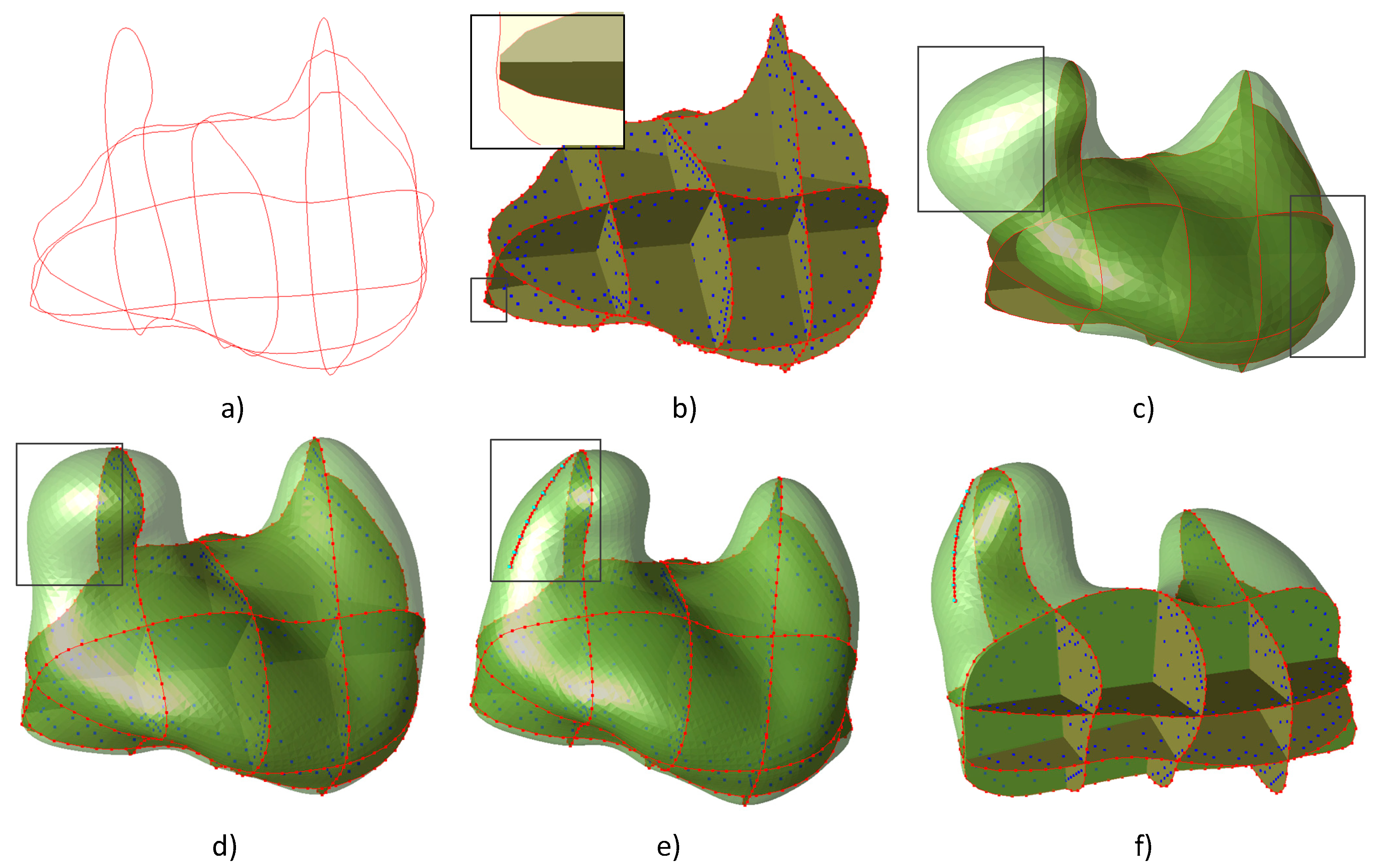
Figure 6.
Reconstructions from input cross sections (a) of a geological example using the method of Liu et al. [18] (c) and the improved method without a constraint line (d) and with a constraint line (e). The geological domain (cutaway view in (f)) is sampled (b) by different function values to form a signed distance field.

Figure 7.
Reconstruction results for multiple types of data sets. These data sets are parallel (a,b) and non-parallel (c–f) cross sections sampled from ground truth objects.
Figure 7.
Reconstruction results for multiple types of data sets. These data sets are parallel (a,b) and non-parallel (c–f) cross sections sampled from ground truth objects.

Figure 8.
Comparison of reconstructions from cross sections (a) using the method of explicit modeling (b), the method of Zou et al. [22] (c), the unconstrained method with (d) and without (e) distance correction), and the improved method (f) with additional constraints. Arrows point to unexpected errors, for which the results do not recover the original shape. Three constraint lines (red) (a) were added to fix the unexpected errors.

Figure 9.
Comparison of running time on several examples. The scale of the time axis is a nonlinear scale (logarithmic).
Figure 9.
Comparison of running time on several examples. The scale of the time axis is a nonlinear scale (logarithmic).

Figure 10.
The inputs (a) and reconstructions with some (b) and more (c) constraints. Two black boxes point to undesired holes (b), constraint lines (blue) (c) were added to fix the topological issues.
Figure 10.
The inputs (a) and reconstructions with some (b) and more (c) constraints. Two black boxes point to undesired holes (b), constraint lines (blue) (c) were added to fix the topological issues.


Table 1.
Common radial basis functions.
| Name of RBFs | Definition |
|---|---|
| Biharmonic | |
| Triharmonic | |
| Multivariate spline | |
| Gaussian | |
| Multiquadric | |
| Inverse multiquadric | |
| Thin-plate spline | |
| Multivariate spline |
Table 2.
Running time of the solution and reconstruction of our algorithm on several examples. Also showing the number of constraints (N), sampling interval in cross sections (), boundary subdivision level (), internal subdivision level (), size of resolution () and relative geometric error (Err.).
Table 2.
Running time of the solution and reconstruction of our algorithm on several examples. Also showing the number of constraints (N), sampling interval in cross sections (), boundary subdivision level (), internal subdivision level (), size of resolution () and relative geometric error (Err.).
| Models | N | Err. | Time (s) | |||||||
|---|---|---|---|---|---|---|---|---|---|---|
| LU | PMC | FMM | SF | |||||||
| Figure 7a | 1082 | 2.9 | 2 | 5 | 0.50 | 0.44% | 3.05 | 163.29 | 0.37 | 0.68 |
| Figure 7b | 2183 | 9.6 | 2 | 5 | 14.71 | 0.21% | 21.71 | 25.04 | 0.97 | 0.32 |
| Figure 7c | 949 | 3.1 | 2 | 5 | 0.50 | 0.71% | 2.12 | 47.18 | 0.25 | 0.62 |
| Figure 7d | 2288 | 3.0 | 2 | 5 | 1.33 | 0.28% | 25.35 | 15.31 | 0.75 | 0.23 |
| Figure 7e | 4125 | 2.0 | 2 | 6 | 4.51 | 0.47% | 121.81 | 27.82 | 2.27 | 0.41 |
| Figure 7f | 3484 | 0.5 | 2 | 6 | 0.80 | 0.89% | 69.65 | 61.24 | 0.99 | 0.39 |
© 2019 by the authors. Licensee MDPI, Basel, Switzerland. This article is an open access article distributed under the terms and conditions of the Creative Commons Attribution (CC BY) license (http://creativecommons.org/licenses/by/4.0/).
Share and Cite
MDPI and ACS Style
Zhong, D.-Y.; Wang, L.-G.; Jia, M.-T.; Bi, L.; Zhang, J. Orebody Modeling from Non-Parallel Cross Sections with Geometry Constraints. Minerals 2019, 9, 229. https://doi.org/10.3390/min9040229
AMA Style
Zhong D-Y, Wang L-G, Jia M-T, Bi L, Zhang J. Orebody Modeling from Non-Parallel Cross Sections with Geometry Constraints. Minerals. 2019; 9(4):229. https://doi.org/10.3390/min9040229
Chicago/Turabian StyleZhong, De-Yun, Li-Guan Wang, Ming-Tao Jia, Lin Bi, and Ju Zhang. 2019. "Orebody Modeling from Non-Parallel Cross Sections with Geometry Constraints" Minerals 9, no. 4: 229. https://doi.org/10.3390/min9040229
Note that from the first issue of 2016, this journal uses article numbers instead of page numbers. See further details here.