Canonical Coordinates for Retino-Cortical Magnification

Abstract

A geometric model for a biologically-inspired visual front-end is proposed, based on an isotropic, scale-invariant two-form field. The model incorporates a foveal property typical of biological visual systems, with an approximately linear decrease of resolution as a function of eccentricity, and by a physical size constant that measures the radius of the geometric foveola, the central region characterized by maximal resolving power. It admits a description in singularity-free canonical coordinates generalizing the familiar log-polar coordinates and reducing to these in the asymptotic case of negligibly-sized geometric foveola or, equivalently, at peripheral locations in the visual field. It has predictive power to the extent that quantitative geometric relationships pertaining to retino-cortical magnification along the primary visual pathway, such as receptive field size distribution and spatial arrangement in retina and striate cortex, can be deduced in a principled manner. The biological plausibility of the model is demonstrated by comparison with known facts of human vision.

1. Introduction

The visual system of humans (and other mammalian species) interfaces the optical world via a sensorium (or visual front-end, the internal embodiment of the visual field) that is characterized by receptive fields, i.e., light sensitive cells, of various sizes and aperture profiles. Scale space theory provides a foundation for a rigorous taxonomy and functional interpretation of visual receptive fields as (exact) non-infinitesimal differential operators. The conjecture that the brain can be seen as a “geometry engine” has been introduced by Koenderink in his seminal papers and has been amply exploited in the image analysis literature [1,2,3,4,5,6,7,8,9,10,11]. The keyword is resolution (or its inverse, scale).

Conventional linear scale space theory, however, typically presumes (scale-wise) uniform sampling, ignoring the foveal properties and real-time dynamics typical of biological visual systems. For the temporal aspects, the reader is again referred to Koenderink for an interesting proposition [12]. The present article concerns the static foveation aspect of the visual front-end, de-emphasizing specific characteristics of visual receptive fields other than the size and spatial arrangement of their effective domains of support.

The visual system of humans shows a roughly linear decrease of visual acuity with eccentricity, is more or less rotationally invariant relative to the foveal point and exhibits a large degree of invariance to object size. Ample empirical evidence supports these claims, including quantitative studies of retino-cortical magnification [13]. Among others, this phenomenon is responsible for the fact that, in the case of humans, about half of the striate cortex is devoted to a foveal region covering only one percent of the visual field. The log-polar mapping arises naturally in simplified models of foveal systems endowed with the aforementioned properties, cf. [14]. Image processing algorithms, as well as space-variant CMOScameras [15,16] have been constructed to mimic this mapping. These dimensionality reducing sampling devices have turned out to be useful in computer vision, as they help to optimize visual tasks, such as time to impact calculations.

However, no previously proposed theory seems to provide a principled account of the spatial organization of the entire retina, including the fovea centralis (the central, avascular zone of the retina with maximal acuity), where the log-polar model breaks down, due to its physically void singularity. This shortcoming is reflected in the design of log-polar mapping algorithms and space-variant cameras, in which one typically employs some heuristics to handle the transition between periphery and central retina.

In this article, based on previous workshop papers [14,17], a model is presented that overcomes the difficulties of the log-polar paradigm. It is based on the same invariance principles, viz. global rotation invariance (with respect to the foveal point) and scale invariance, but explicitly incorporates a physical resolution limitation. The model admits so-called canonical coordinates, inducing a natural discrete grid for operational representation in software, hardware or biological “wetware”. Its biological merits will be discussed by comparison with known facts on human vision. To guide the reader not familiar with the biological terminology used in this article, a glossary of relevant biological terms has been appended.

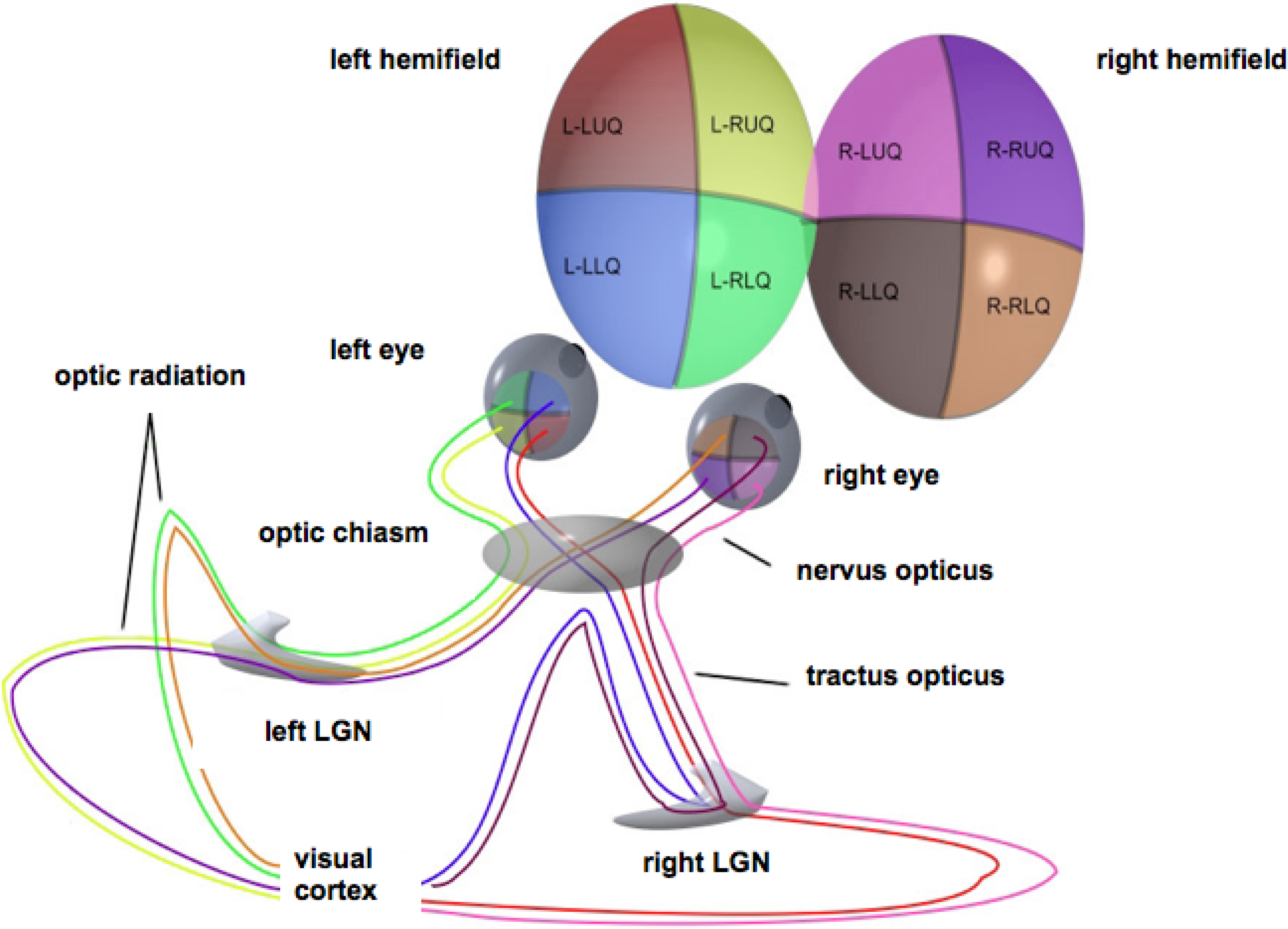
For simplicity, stereopsis will be ignored. The retina will be modeled as a flat disk, representing the domain of definition of the full visual field. This field comprises two hemifields, each of which projects onto a (contralateral) hemiretina, in turn projecting retinotopically to the primary visual (or striate) cortex through the optic radiation via the subcortical lateral geniculate nucleus. Thus, each lateral part of the visual cortex reflects the contralateral visual hemifield [13], cf. the sketch in Figure 1.

2. Theory

2.1. Modeling the Sensorium

Consider the basic scale invariant non-exact (the barred symbol, $đ$, is used to stress the anholonomic nature of the one-forms) one-forms:

$$đ\xi =\frac{dx}{\sqrt{x^2+y^2+a^2}}\text{and}đ\eta =\frac{dy}{\sqrt{x^2+y^2+a^2}}$$

(1)

in which $(x,y)\in {\mathbb{R}}^2$ are Cartesian coordinates. From an operational point of view, one could regard these as locally adaptive measurement rods, with the help of which, one may assign a numeric value to a vector depending on the base point to which it is attached. More precisely, if $v(x,y)=v^x(x,y)e_x+v^y(x,y)e_y$ is such a vector, “living” at base point $(x,y)$ and expressed relative to globally-defined Cartesian unit vectors $e_x$ and $e_y$, then:

$$đ\xi \left(v\right)=\frac{v^x(x,y)}{\sqrt{x^2+y^2+a^2}}\text{and}đ\eta \left(v\right)=\frac{v^y(x,y)}{\sqrt{x^2+y^2+a^2}}$$

(2)

Figure 1. Schematic representation of the optic pathways from each of the four quadrants of view for both eyes. Adapted from Wikimedia Commons, original illustration by Ratznium. LGN, lateral geniculate nucleus.

Figure 1. Schematic representation of the optic pathways from each of the four quadrants of view for both eyes. Adapted from Wikimedia Commons, original illustration by Ratznium. LGN, lateral geniculate nucleus.

These numeric values could be interpreted to represent the “visual significance” of the respective Cartesian vector components depending on the position in the visual field. Clearly, in order to be equally significant, the components of a vector at some peripheral location (large $\sqrt{x^2+y^2+a^2}$) will need to be larger than those of a more central one (small $\sqrt{x^2+y^2+a^2}$). The reason for this is to geometrically express the roughly linear increase of typical receptive field size (with a concomitant linear decrease of spatial resolving power) as a function of eccentricity $\sqrt{x^2+y^2}$. The (small) physical size parameter $a>0$ is needed to avoid a non-physical singularity at the center. Its visual significance will become apparent below.

We will confine the region of interest to a disk of radius R, which represents the radius of the geometric retina($\sqrt{x^2+y^2}\le R$). The parameter, a, represents a transient radius separating the geometric foveola(the geometric foveola is a construct of our model, to be distinguished from the biological foveolain the mammalian retina; terminology betrays a modest amount of foresight) ($\sqrt{x^2+y^2}\le a$) from its periphery($\sqrt{x^2+y^2}>a$).

The one-forms of Equation (1) induce a scale invariant area two-form, geometrically representing a spatially-weighted area of support (regardless of shape) of a Euclidean sensory element, $dx\wedge dy$, at position $(x,y)$ relative to the foveal center:

$$\mathsf{\Omega }=\sqrt{g}dx\wedge dy=đ\xi \wedge đ\eta$$

(3)

in which:

$$\sqrt{g}=\frac{1}{x^2+y^2+a^2}$$

(4)

is the square root of the metric determinant associated with the two-dimensional spatial metric:

$$\text{G}=\frac{dx\otimes dx+dy\otimes dy}{x^2+y^2+a^2}=đ\xi \otimes đ\xi +đ\eta \otimes đ\eta$$

(5)

Again, the number in Equation (4) reflects the fact that a peripheral receptive field will need to have a larger area of support in order to be treated on par with a similar one closer to the foveal center.

As an aside, recall that the every two-dimensional Riemannian manifold is conformally flat and that the Ricci curvature tensor, $\mathrm{Ric}$, is always proportional to the metric tensor, viz.:

$${\mathcal{R}}_{\mu \nu }=\frac{1}{2}\mathcal{R}{g}_{\mu \nu }(\mu ,\nu =1,2)$$

(6)

in which ${\mathcal{R}}_{\mu \nu }$ and $g_{\mu \nu }$ are the components of $\mathrm{Ric}$ and G, respectively. For the case at hand, Equation (5), the space-variant Ricci scalar (equal to twice the Gaussian curvature) equals:

$$\mathcal{R}(x,y)=\frac{4a^2}{x^2+y^2+a^2}$$

(7)

This curvature scalar assumes appreciable values within the fovea centralis. The point of departure in previous work [14] was based on the assumption that $\mathcal{R}=0$ for all $(x,y)\ne (0,0)$. Combined with the aforementioned symmetries and applied to a conformally flat metric, this requirement admits a family of metrics, of which Equation (5) is a particular member, only if $a=0$, leaving a spurious singularity at the origin. It is clearly not compatible with our regularized metric with $a>0$.

2.2. Modeling Retino-Cortical Magnification

Consider the area (measured by the Riemannian metric of Equation (5)) of an infinitesimally narrow ring $\delta \mathrm{\Gamma }:\rho <\sqrt{x^2+y^2}<\rho +\delta \rho$ around the fovea:

$$\delta V\left(\rho \right)={\int \int }_{\delta \mathrm{\Gamma }}đ\xi \wedge đ\eta =\delta \rho {\int }_0^{2\pi }\frac{\rho }{{\rho }^2+a^2}d\varphi =\frac{2\pi \rho \delta \rho }{{\rho }^2+a^2}$$

(8)

Geometrically, the quantity:

$$V^{\prime }\left(\rho \right)=\frac{2\pi \rho }{{\rho }^2+a^2}\stackrel{\mathrm{def}}{=}P\left(\rho \right)$$

(9)

measures the (Riemannian) perimeter of a the circle of radius ρ around the fovea. It is easy to see that there exists a maximal circle, with perimeter $P_{+}=P\left(a\right)$, demarcating the transition ${\rho }_{+}=a$ between the geometric foveola and periphery (whether this transient circle has a distinguished functional role in mammalian vision is not clear, but anatomical evidence does show a fairly sharp demarcation of the biological foveola [13]).

If we normalize $V\left(\rho \right)$, such that $V\left(0\right)=0$, and introduce the dimensionless quantities:

$$v^{\prime }(t,T)=\frac{\partial v(t,T)}{\partial t}$$

(10)

and:

$$v(t,T)=\frac{V\left(at\right)}{V\left(aT\right)}$$

(11)

with $0\le t\le T$, and:

$$t=\frac{\rho }{a}\text{and}T=\frac{R}{a}$$

(12)

then:

$$v(t,T)=\frac{ln\left(1+t^2\right)}{ln\left(1+T^2\right)}$$

(13)

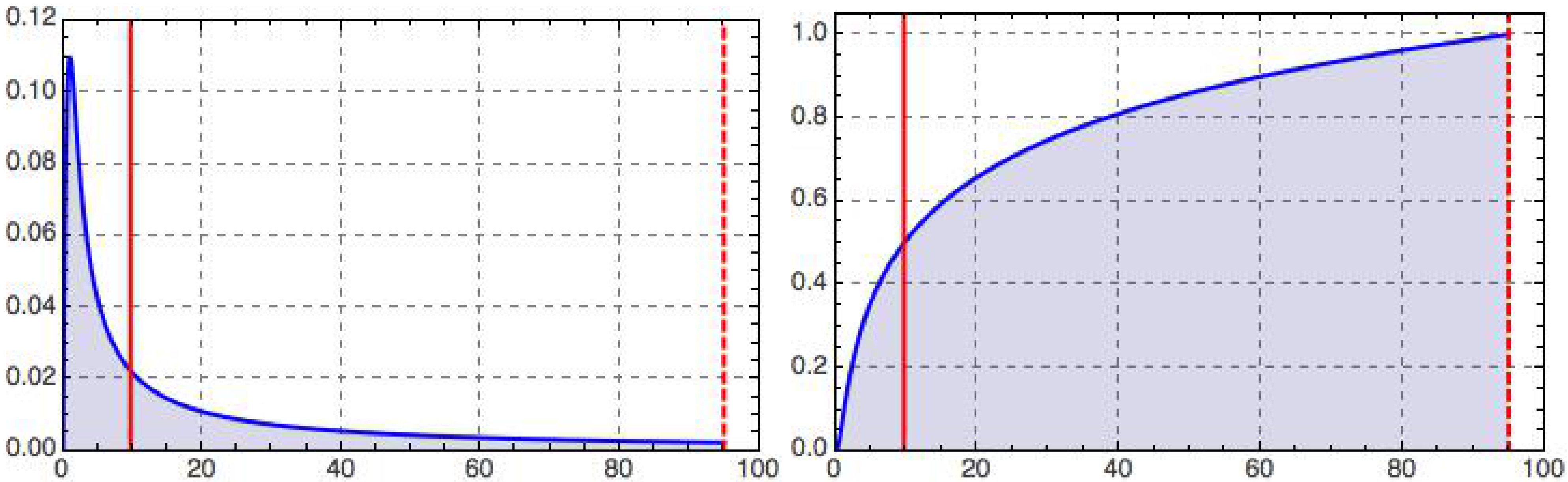
This integrated retino-cortical magnificationmeasures the relative capacity dedicated to the central region inside a foveal disk of radius $\rho =at$ relative to that of the full retina. Limiting cases are clearly $v(0,T)=0$ and $v(T,T)=1$. For the foveola, we have $v(t_{+}\stackrel{\mathrm{def}}{=}1,T)=ln2/ln(1+T^2)$; cf. Figure 2 for an illustration.

To verify the biological plausibility of our model, consider the case of a peripheral ring with the same processing capacity as the enclosed foveal disk, i.e., Equation (13) with equipartitioning radius${\rho }_{\frac{1}{2}}=a{t}_{\frac{1}{2}}$ defined, such that:

$$v(t_{\frac{1}{2}},T)\stackrel{\mathrm{def}}{=}\frac{1}{2}$$

(14)

A straightforward computation yields:

$$t_{\frac{1}{2}}=\sqrt{\sqrt{1+T^2}-1}\approx \sqrt{T}$$

(15)

in which the approximation reflects the phenomenological case, $T\gg 1$. In other words, under this assumption, the theoretical equipartitioning radius approximately equals the geometric mean of the radii of the geometric foveola and geometric retina:

$${\rho }_{\frac{1}{2}}\approx \sqrt{aR}$$

(16)

Generalizing Equations (14)–(16), we may define the α-partitioning radii ${\rho }_{\alpha }=a{t}_{\alpha }$, via:

$$v(t_{\alpha },T)\stackrel{\mathrm{def}}{=}\alpha \text{for }0\le \alpha \le 1$$

(17)

yielding (the approximations hold for not too small α, i.e., well outside the geometric foveola):

$$t_{\alpha }=\sqrt{{(1+T^2)}^{\alpha }-1}\approx T^{\alpha }(T\gg 1)$$

(18)

or, in terms of physical length scales,

$${\rho }_{\alpha }\approx a^{1-\alpha }{R}^{\alpha }(R\gg a)$$

(19)

This prediction likewise admits experimental verification once consistent values of a and R are at hand.

Vice versa, we may use Equations (16)–(19) to definethe constant, a, given empirical data for R and, say, ${\rho }_{\frac{1}{2}}$. For instance, in the case of humans, it is known that about half of the striate cortex is devoted to the portion of the retina that lies within $7^{\circ }$–$8^{\circ }$ of the fovea [13]. Assuming that the striate cortex has a homogeneous distribution of similar visual cells, the fractional size within it occupied by the retinotopically-mapped central portion of the visual field will be tantamount to its fractional processing capacity. A typical retina measures [18] $R\approx 21\text{mm}$; $1^{\circ }$ of visual angle corresponds to approximately $288\mu \mathrm{m}$. The monocular visual field covers approximately ${160}^{\circ }\times {175}^{\circ }$ ($\text{width}\times \text{height}$ [19]), or roughly ${(85\pm 5)}^{\circ }$ in eccentricity when approximated by an isotropic figure for our purposes (Hartridge [20] reports a functional limit on visual field eccentricity of ${104}^{\circ }$). With these figures, we have (for the biological counterparts of the quantities involved) $t_{\frac{1}{2}}/T={\rho }_{\frac{1}{2}}/R\approx 0.1024$, from which one deduces with the help of Equations (12) and (15) that $a={(t_{\frac{1}{2}}/T)}^{2}R\approx 0.22\text{mm}$. The phenomenological value $T={(R/{\rho }_{\frac{1}{2}})}^2\approx 95$ used in Figure 2 justifies our assumption, $T\gg 1$, and the predicted size of the geometric foveola happens to agree remarkably well with that of the human foveola (Rodieck ([13], Chapter 9) reports a value of $0.20\text{mm}$), which gives us a biological interpretation of the constant, a, and, at the same time, justifies the name “geometric foveola”; cf. Figure 3.

In the next section, we consider the modification of the log-polar map by taking into account the physical resolution limitation of the fovea centralis and show how the log-polar map emerges asymptotically.

Figure 2. Retino-cortical magnification, $V^{\prime }(t,T)$ (left), and its integral, $V(t,T)$ (right), as a function of dimensionless eccentricity, t, illustrated for the case $T=95$ (dashed vertical line); recall Equations (12)–(15). The peak on the left occurs at $t_{+}=1$ and marks the border ${\rho }_{+}=a$ of the geometric foveola. The half maximum on the right is reached at $t_{\frac{1}{2}}\approx \sqrt{T}$, corresponding to the geometric equipartitioning radius (left vertical line), ${\rho }_{\frac{1}{2}}\approx \sqrt{aR}$. With our choice of parameters (motivated in the text), the tiny geometric foveola has a relative processing capacity $v(t_{+}=1,T=95)\approx 8\%$; recall Equation (13).

Figure 2. Retino-cortical magnification, $V^{\prime }(t,T)$ (left), and its integral, $V(t,T)$ (right), as a function of dimensionless eccentricity, t, illustrated for the case $T=95$ (dashed vertical line); recall Equations (12)–(15). The peak on the left occurs at $t_{+}=1$ and marks the border ${\rho }_{+}=a$ of the geometric foveola. The half maximum on the right is reached at $t_{\frac{1}{2}}\approx \sqrt{T}$, corresponding to the geometric equipartitioning radius (left vertical line), ${\rho }_{\frac{1}{2}}\approx \sqrt{aR}$. With our choice of parameters (motivated in the text), the tiny geometric foveola has a relative processing capacity $v(t_{+}=1,T=95)\approx 8\%$; recall Equation (13).

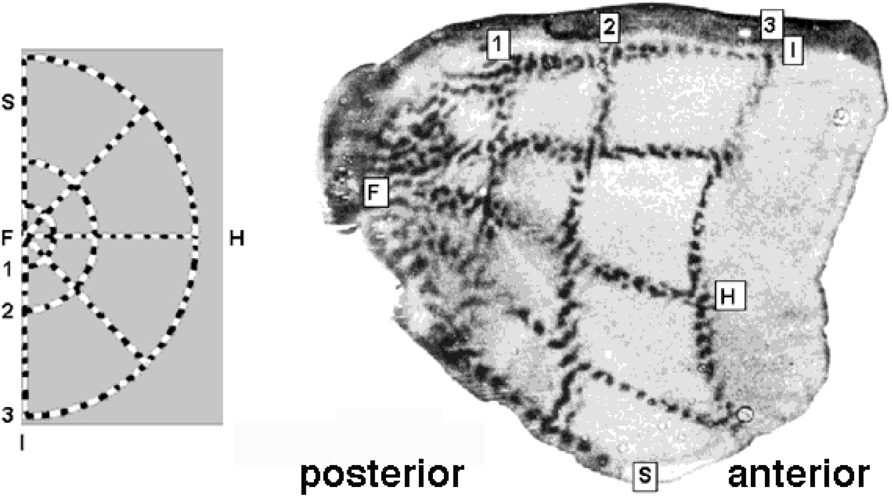
Figure 3. Retino-cortical mapping of macaque monkey. (Left) Retina with spoke-wheel stimulus. (Right) Stimulus image retinotopically mapped onto the posterior part of (hemifield) striate cortex, a.k.a. calcarine sulcus. Source: Tootell et al. [21].

Figure 3. Retino-cortical mapping of macaque monkey. (Left) Retina with spoke-wheel stimulus. (Right) Stimulus image retinotopically mapped onto the posterior part of (hemifield) striate cortex, a.k.a. calcarine sulcus. Source: Tootell et al. [21].

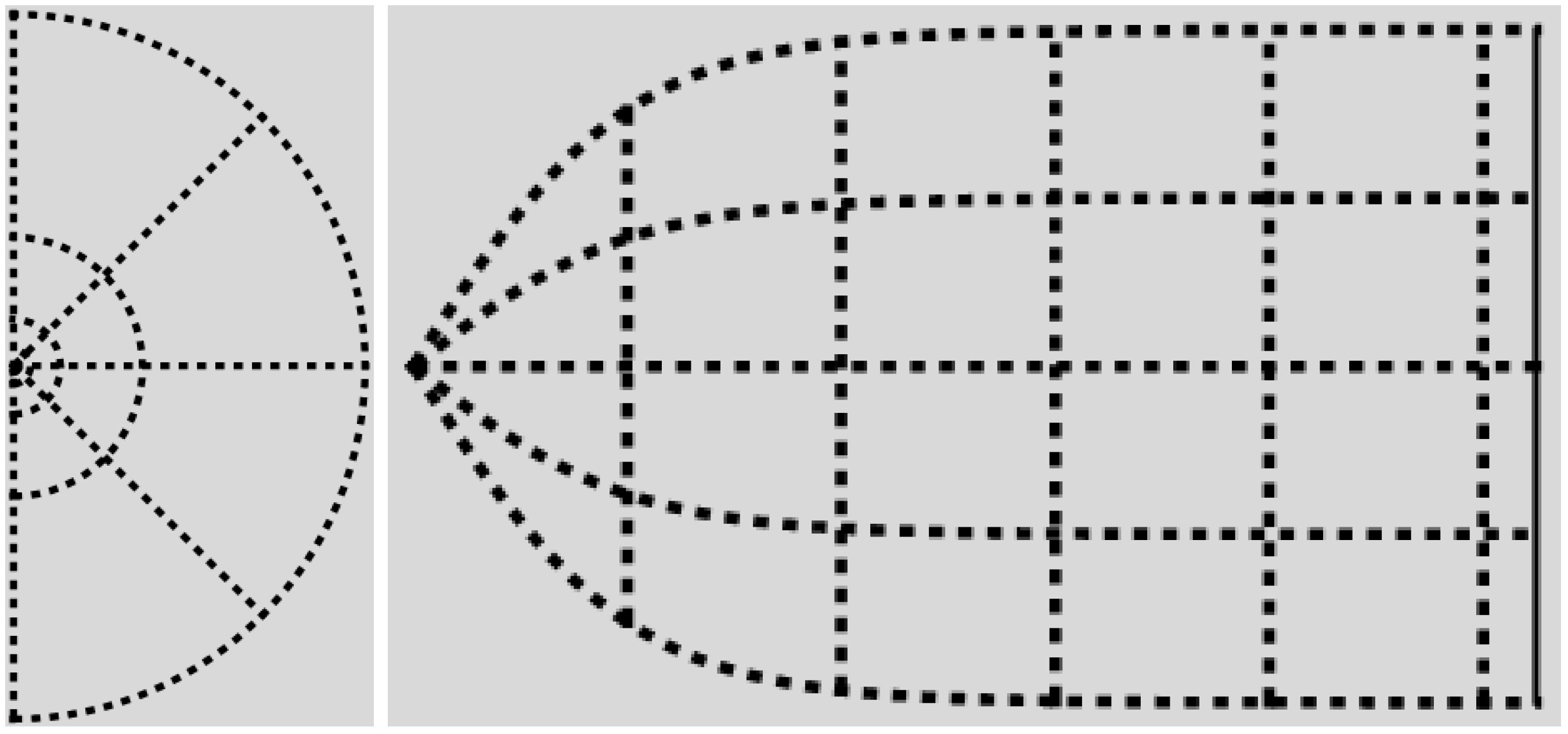
2.3. Canonical Coordinates

Retino-cortical magnification can be conveniently described in terms of canonical coordinates(recall that the primary visual cortex on one side of the brain represents a hemifield, hence the bounds on ϕ):

$$\left\{\begin{array}{cccc}{\displaystyle p}\hfill & =\hfill & {\displaystyle \text{arcsinh}t=ln\left(t+\sqrt{1+t^2}\right)}\hfill & ,\hfill \\ {\displaystyle q}\hfill & =\hfill & {\displaystyle \frac{t\varphi }{\sqrt{1+t^2}}}\hfill & (0\le t\le T,-\frac{\pi }{2}\le \varphi \le \frac{\pi }{2})\hfill \end{array}\right.$$

(20)

Using these canonical coordinates, it follows that the basic area two-form (recall Equation (3)) can be expressed as the wedge product of holonomic one-forms, warranting the attribute “canonical”:

$$\mathsf{\Omega }=dp\wedge dq$$

(21)

Note that near the foveal point, we have:

$$\left\{\begin{array}{cccc}{\displaystyle p}\hfill & \approx \hfill & {\displaystyle t}\hfill & \hfill \\ {\displaystyle q}\hfill & \approx \hfill & {\displaystyle t\varphi }\hfill & (0\le t\ll 1,-\frac{\pi }{2}\le \varphi \le \frac{\pi }{2})\hfill \end{array}\right.$$

(22)

In the periphery, we reobtain the familiar log-polar coordinates (up to an irrelevant offset):

$$\left\{\begin{array}{cccc}{\displaystyle p}\hfill & \approx \hfill & {\displaystyle ln2t}\hfill & \hfill \\ {\displaystyle q}\hfill & \approx \hfill & {\displaystyle \varphi }\hfill & (1\ll t\le T,-\frac{\pi }{2}\le \varphi \le \frac{\pi }{2})\hfill \end{array}\right.$$

(23)

The physical part of the $(p,q)$-domain is reminiscent of the actually observed shape of the cortical surface of V1; compare Figure 3 and Figure 4.

Figure 4. The canonical $(p,q)$-domain is the region between the graphs of $q_{\pm \frac{\pi }{2}}=\pm \frac{\pi }{2}tanhp$ and the lines $p=0$ and $p=\mathrm{arcsinh}T$. On the left, $(t,\varphi )$ are dimensionless radial and azimuthal coordinates. On the right, the canonical $(p,q)$-coordinates are plotted as Cartesian coordinates, with p on the horizontal axis. Recall Equation (28), and compare with Figure 3.

Figure 4. The canonical $(p,q)$-domain is the region between the graphs of $q_{\pm \frac{\pi }{2}}=\pm \frac{\pi }{2}tanhp$ and the lines $p=0$ and $p=\mathrm{arcsinh}T$. On the left, $(t,\varphi )$ are dimensionless radial and azimuthal coordinates. On the right, the canonical $(p,q)$-coordinates are plotted as Cartesian coordinates, with p on the horizontal axis. Recall Equation (28), and compare with Figure 3.

Expressed in canonical coordinates, the retino-cortical metric, Equation (5), looks rather more cumbersome:

$$\text{G}=\left(1+\frac{4q^2}{{sinh}^2\left(2p\right)}\right)dp\otimes dp-\frac{4q}{sinh\left(2p\right)}dp\otimes dq+dq\otimes dq$$

(24)

It is evident that the $(p,q)$-coordinate lines do not intersect perpendicularly, unlike with log-polar coordinates; cf. Figure 4. For the angle of intersection, α, at a fiducial point $(p,q)$, we have:

$$cos\alpha =\frac{-2q}{\sqrt{4q^2+{sinh}^2\left(2p\right)}}$$

(25)

For peripheral points, this is close to zero:

$$cos\alpha \approx -\frac{a^2\varphi }{{\rho }^2}\approx 0(\rho \gg a)$$

(26)

For central points, on the other hand, we have:

$$cos\alpha \approx -\frac{\varphi }{\sqrt{1+{\varphi }^2}}(\rho \ll a)$$

(27)

independent of eccentricity, revealing the non-orthogonal intersection of canonical coordinate lines away from the horizon ($\varphi =0$). The deviation from orthogonality remains nonetheless fairly small almost everywhere, reaching its maximum at the foveal point, with an intersection angle still close to ${60}^{\circ }$. Typical measurements, such as Figure 3, lack resolving power to delineate foveal details in the most posterior part of the striate cortex and, thus, remain indecisive.

Let ${\mathrm{\Gamma }}_T$ denote the full retinal domain. In $(p,q)$-space this is the area in-between the graphs of:

$$q_{\pm \frac{\pi }{2}}\left(p\right)=\pm \frac{\pi }{2}tanhp$$

(28)

and the lines $p=0$ and $p=\text{arcsinh}T$ (to see this, express q as a function of p and parameter ϕ using Equation (20), and consider the boundary values ${\varphi }_{\pm }=\pm \pi /2$). By the same token, if ${\mathrm{\Gamma }}_t$ denotes the fraction of the retinal domain on the left of the line $p=\text{arcsinh}t$, then a straightforward computation yields:

$$\frac{{\int }_{{\mathrm{\Gamma }}_t}\mathsf{\Omega }}{{\int }_{{\mathrm{\Gamma }}_T}\mathsf{\Omega }}=\frac{{\int }_0^{\text{arcsinh}t}{q}_{\frac{\pi }{2}}\left(p\right)dp}{{\int }_0^{\text{arcsinh}T}{q}_{\frac{\pi }{2}}\left(p\right)dp}=v(t,T)$$

(29)

reproducing Equation (13) as expected. This confirms that the $(p,q)$-coordinates of Equation (20) are indeed more natural than the commonly used log-polar coordinates. The latter arise in the limit of vanishing a. As such, log-polar coordinates fail to describe both foveal, as well as transient behavior, and are suited only for the peripheral field. Although the periphery represents by far the largest part of the visual field, it is much less significant in the visual brain.

As a final remark, note that, by construction, $(p,q)$-space is most naturally discretized by a uniform sampling (with grid constants $\mathsf{\Delta }p$ and $\mathsf{\Delta }q$ of fixed aspect ratio). Biologically, one expects this to be reflected in a uniform spatial layout and the functional similarity of cortical receptive fields in the entire primary visual cortex.

3. Conclusion and Discussion

We have established a biologically plausible geometric model for an isotropic, scale-invariant foveal system that incorporates physical resolution limitations. The model is naturally described in terms of a canonical coordinate map that generalizes the familiar log-polar map typically used in the context of foveal systems. Unlike the latter, however, the generalized map has a globally valid domain of definition and handles the transition from the peripheral field (the classical log-polar regime) to fovea centralis in a graceful manner.

The model is consistent with certain known facts of biological vision, notably retino-cortical magnification. Other quantitative predictions may be inferred from it to assess its biological merits and, perhaps, even to predict hitherto unexplored properties about biological foveal systems. Empirical verification, however, will require methods of high resolving power in order to discriminate details within the foveola and its corresponding image in the striate cortex in order to be able to verify or refute the canonical paradigm stipulated in this article.

An important property that has not been accounted for in our model is the fact that at each spatial location in the retina or striate cortex, there exist ensembles of similar receptive fields differing only in size. The proposed model describes the inherent resolution limitation of the visual system by considering “typical” (e.g., minimal) size as a function of eccentricity. Geometric models that do take into account the local multiscale nature of the visual system have been proposed in the context of artificial and biological vision (cf. the Riemannian structure proposed by Eberly et al. [22] and, in a different application context, van Wijk and Nuij [23]; and the affine structure stipulated by Florack [24]). Koenderink has considered the surface geometry of an intensity cross-section induced by a visual stimulus [25]. Many intriguing questions remain, such as how these geometries (one of which does not necessarily exclude another!) contribute to our perception of the (geometry of the) visual world “outside”; cf. Koenderink et al. [26,27]. However, even rudimentary questions remain essentially unsolved, such as how the visual system, without the infinite regression inevitably arising from the tacit ministration of a homunculus—a little (wo)man inside the brain viewing an internal screen—is able to derive topological expertise from a massive body of essentially unordered, parallel neural signals [28].

References

- Duits, R.; Florack, L.; de Graaf, J.; ter Haar Romeny, B. On the axioms of scale space theory. J. Math. Imaging Vis. 2004, 20, 267–298. [Google Scholar] [CrossRef]
- Florack, L.M.J.; Haar Romeny, B.M.; ter Koenderink, J.J.; Viergever, M.A. Linear scale-space. J. Math. Imaging Vis. 1994, 4, 325–351. [Google Scholar] [CrossRef]
- Florack, L.M.J. Image Structure: Computational Imaging and Vision Series; Kluwer Academic Publishers: Dordrecht, The Netherlands, 1997; Volume 10. [Google Scholar]
- Iijima, T. Basic theory on normalization of a pattern (in case of typical one-dimensional pattern). Bull. Electr. Lab. 1962, 26, 368–388. (in Japanese). [Google Scholar]
- Koenderink, J.J. The structure of images. Biol. Cybern. 1984, 50, 363–370. [Google Scholar] [CrossRef] [PubMed]
- Koenderink, J.J.; van Doorn, A.J. Representation of local geometry in the visual system. Biol. Cybern. 1987, 55, 367–375. [Google Scholar] [CrossRef] [PubMed]
- Koenderink, J.J.; van Doorn, A.J. Operational significance of receptive field assemblies. Biol. Cybern. 1988, 58, 163–171. [Google Scholar] [CrossRef] [PubMed]
- Koenderink, J.J.; van Doorn, A.J. Receptive field families. Biol. Cybern. 1990, 63, 291–298. [Google Scholar] [CrossRef]
- Koenderink, J.J. The brain a geometry engine. Psychol. Res. 1990, 52, 122–127. [Google Scholar] [CrossRef] [PubMed]
- Weickert, J.A.; Ishikawa, S.; Imiya, A. Linear scale-space has first been proposed in Japan. J. Math. Imaging Vis. 1999, 10, 237–252. [Google Scholar] [CrossRef]
- Witkin, A.P. Scale-Space Filtering. In Proceedings of the International Joint Conference on Artificial Intelligence, Karlsruhe, Germany, 8–12 August 1983; pp. 1019–1022.
- Koenderink, J.J. Scale-time. Biol. Cybern. 1988, 58, 159–162. [Google Scholar] [CrossRef]
- Rodieck, R.W. The First Steps in Seeing; Sinauer Associates, Inc.: Sunderland, MA, USA, 1998. [Google Scholar]
- Florack, L.M.J. A Geometric Model for Cortical Magnification. In Biologically Motivated Computer Vision: Lecture Notes in Computer Science; Proceedings of the First IEEE International Workshop, BMCV 2000, Seoul, Korea, 15–17 May 2000; Lee, S.W., Bülthoff, H.H., Poggio, T., Eds.; Springer-Verlag: Berlin, Germany, 2000; Volume 1811, pp. 574–583. [Google Scholar]
- Tistarelli, M.; Sandini, G. On the advantages of polar and log-polar mapping for direct estimation of time-to-impact from optical flow. IEEE Trans. Pattern Anal. Mach. Intell. 1993, 15, 401–416. [Google Scholar] [CrossRef]
- Ho, C.G.; Young, R.C.D.; Chatwin, C.R. Sensor geometry and sampling methods for space-variant image processing. Pattern Anal. Appl. 2002, 5, 369–384. [Google Scholar] [CrossRef]
- Florack, L.M.J. Modeling Foveal Vision. In Scale Space and Variational Methods in Computer Vision: Lecture Notes in Computer Science; Proceedings of the First International Conference, SSVM 2007, Ischia, Italy, 30 May–2 June 2007; Sgallari, F., Murli, A., Paragios, N., Eds.; Springer-Verlag: Berlin, Germany, 2007; Volume 4485, pp. 919–928. [Google Scholar]
- webvision.med.utah.edu. Available online: http://webvision.med.utah.edu (accessed on 21 February 2014).
- Wandell, B.A. Foundations of Vision; Sinauer Associates, Inc.: Sunderland, MA, USA, 1995. [Google Scholar]
- Hartridge, H. The limit to peripheral vision. J. Physiol. 1919, 53, 17. [Google Scholar]
- Tootell, R.B.H.; Switkes, E.; Silverman, M.S.; Hamilton, S.L. Functional anatomy of macaque striate cortex. II. Retinotopic organization. J. Neurosci. 1988, 8, 1531–1568. [Google Scholar] [PubMed]
- Eberly, D. A Differential Geometric Approach to Anisotropic Diffusion. In Geometry-Driven Diffusion in Computer Vision: Computational Imaging and Vision Series; ter Haar Romeny, B.M., Ed.; Kluwer Academic Publishers: Dordrecht, The Netherlands, 1994; Volume 1, pp. 371–392. [Google Scholar]
- Van Wijk, J.J.; Nuij, W.A.A. Smooth and Efficient Zooming and Panning. In Proceedings of the IEEE Symposium on Information Visualization (InfoVis’2003), Seattle, WA, USA, 20–21 October 2003; Munzner, T., North, S., Eds.; IEEE Computer Society Press: Washington, DC, USA, 2003; pp. 15–22, Best paper award. [Google Scholar]
- Florack, L.M.J. Deep Structure from a Geometric Point of View. In Deep Structure Singularities and Computer Vision: Lecture Notes in Computer Science; Fogh Olsen, O., Florack, L.M.J., Kuijper, A., Eds.; Springer-Verlag: Berlin/Heidelberg, Germany, 2005; Volume 3753, pp. 135–145. [Google Scholar]
- Koenderink, J.J. A Generic Framework for Image Geometry. In Proceedings of the Conference on Applied Geometrical Algebras in Computer Science and Engineering, AGACSE 2001, Newnham, UK, 9–13 July 2001; Dorst, L., Doran, C., Lasenby, J., Eds.; Birkhaüser: Boston, MA, USA, 2002; pp. 319–332. [Google Scholar]
- Koenderink, J.J.; van Doorn, A.J. Exocentric Pointing; Cambridge University Press: Cambridge, UK, 1998; pp. 295–313. [Google Scholar]
- Koenderink, J.J.; van Doorn, A.J.; Lappin, J.S. Direct measurement of the curvature of visual space. Perception 2000, 29, 69–79. [Google Scholar] [CrossRef] [PubMed]
- Koenderink, J.J. The Concept of Local Sign. In Limits in Perception; Van Doorn, A.J., van der Grind, W.A.P.F.L., Koenderink, J.J., Eds.; VNU Science Press: Utrecht, The Netherlands, 1984; pp. 495–547. [Google Scholar]
Appendix: Biological Terms
avascular zone the central region of the retina without blood vessels, roughly coinciding with the fovea.
eccentricity the radial distance from the foveal center, usually measured in degrees.
fovea (centralis) the central part of the retina, accounting for sharp vision.
foveola the central part of the fovea, accounting for the highest visual acuity.
lateral geniculate nucleus the relay center for visual information in-between the retina and V1, cf. Figure 1.
LGN lateral geniculate nucleus.
optic radiation a.k.a. the geniculostriate pathway; the collection of axons connecting LGN and V1, cf. Figure 1.
primary visual cortex part of the cerebral cortex responsible for visual processing, cf. Figure 1.
receptive field the support region and sensitivity profile of a light-sensitive cell.
retina the light-sensitive inner surface of the eye.
retinotopic mapping mapping (i.c.retina to cortex) preserving neighborhood relations, cf. Figure 3 and Figure 4.
striate cortex same as the primary visual cortex.
V1 same as the primary visual cortex.
© 2014 by the author; licensee MDPI, Basel, Switzerland. This article is an open access article distributed under the terms and conditions of the Creative Commons Attribution license (http://creativecommons.org/licenses/by/3.0/).
Share and Cite
MDPI and ACS Style
Florack, L. Canonical Coordinates for Retino-Cortical Magnification. Axioms 2014, 3, 70-81. https://doi.org/10.3390/axioms3010070
AMA Style
Florack L. Canonical Coordinates for Retino-Cortical Magnification. Axioms. 2014; 3(1):70-81. https://doi.org/10.3390/axioms3010070
Chicago/Turabian StyleFlorack, Luc. 2014. "Canonical Coordinates for Retino-Cortical Magnification" Axioms 3, no. 1: 70-81. https://doi.org/10.3390/axioms3010070