Rough Neutrosophic Digraphs with Application


1
Department of Mathematics, University of the Punjab, New Campus, Lahore 54590, Pakistan
2
Mathematics & Science Department, University of New Mexico, 705 Gurley Ave., Gallup, NM 87301, USA
*
Author to whom correspondence should be addressed.
Axioms 2018, 7(1), 5; https://doi.org/10.3390/axioms7010005
Submission received: 5 December 2017
/
Revised: 14 January 2018
/
Accepted: 15 January 2018
/
Published: 18 January 2018
(This article belongs to the Special Issue Neutrosophic Multi-Criteria Decision Making)
Abstract
:A rough neutrosophic set model is a hybrid model which deals with vagueness by using the lower and upper approximation spaces. In this research paper, we apply the concept of rough neutrosophic sets to graphs. We introduce rough neutrosophic digraphs and describe methods of their construction. Moreover, we present the concept of self complementary rough neutrosophic digraphs. Finally, we consider an application of rough neutrosophic digraphs in decision-making.
MSC:
03E72; 68R10; 68R051. Introduction
Smarandache [1] proposed the concept of neutrosophic sets as an extension of fuzzy sets [2]. A neutrosophic set has three components, namely, truth membership, indeterminacy membership and falsity membership, in which each membership value is a real standard or non-standard subset of the nonstandard unit interval ([3]), where , , is an infinitesimal number . To apply neutrosophic set in real-life problems more conveniently, Smarandache [3] and Wang et al. [4] defined single-valued neutrosophic sets which takes the value from the subset of . Actually, the single valued neutrosophic set was introduced for the first time by Smarandache in 1998 in [3]. Ye [5] considered multicriteria decision-making method using the correlation coefficient under single-valued neutrosophic environment. Ye [6] also presented improved correlation coefficients of single valued neutrosophic sets and interval neutrosophic sets for multiple attribute decision making.
Rough set theory was proposed by Pawlak [7] in 1982. Rough set theory is useful to study the intelligence systems containing incomplete, uncertain or inexact information. The lower and upper approximation operators of rough sets are used for managing hidden information in a system. Therefore, many hybrid models have been built, such as soft rough sets, rough fuzzy sets, fuzzy rough sets, soft fuzzy rough sets, neutrosophic rough sets, andrough neutrosophic sets, for handling uncertainty and incomplete information effectively. Dubois and Prade [8] introduced the notions of rough fuzzy sets and fuzzy rough sets. Liu and Chen [9] have studied different decision-making methods. Broumi et al. [10] introduced the concept of rough neutrosophic sets. Yang et al. [11] proposed single valued neutrosophic rough sets by combining single valued neutrosophic sets and rough sets, and established an algorithm for decision-making problem based on single valued neutrosophic rough sets on two universes. Mordeson and Peng [12] presented operations on fuzzy graphs. Akram et al. [13,14,15,16] considered several new concepts of neutrosophic graphs with applications. Zafer and Akram [17] introduced a novel decision-making method based on rough fuzzy information. In this research study, we apply the concept of rough neutrosophic sets to graphs. We introduce rough neutrosophic digraphs and describe methods of their construction. Moreover, we present the concept of self complementary rough neutrosophic digraphs. We also present an application of rough neutrosophic digraphs in decision-making.
2. Rough Neutrosophic Digraphs
Definition 1.
[4] Let Z be a nonempty universe. A neutrosophic set N on Z is defined as follows:
where the functions :Z→ represent the degree of membership, the degree of indeterminacy and the degree of falsity.
Definition 2.
[7] Let Z be a nonempty universe and R an equivalence relation on Z.A pair is called an approximation space. Let be a subset of Z and the lower and upper approximations of in the approximation space denoted by and are defined as follows:
where denotes the equivalence class of R containing x. A pair is called a rough set.
Definition 3.
[10] Let Z be a nonempty universe and R an equivalence relation on Z. Let N be a neutrosophic set(NS) on Z. The lower and upper approximations of N in the approximation space denoted by and are defined as follows:
where,
A pair is called a rough neutrosophic set.
We now define the concept of rough neutrosophic digraph.
Definition 4.
Let be a nonempty set and R an equivalence relation on . Let V be a NS on , defined as
Then, the lower and upper approximations of V represented by and , respectively, are characterized as NSs in such that ,
where,
Let and S an equivalence relation on such that
Let E be a neutrosophic set on defined as
such that
Then, the lower and upper approximations of E represented by and , respectively, are defined as follows
where,
A pair is called a rough neutrosophic relation.
Definition 5.
A rough neutrosophic digraph on a nonempty set is a four-ordered tuple such that
- (a)
- R is an equivalence relation on ;
- (b)
- S is an equivalence relation on ;
- (c)
- is a rough neutrosophic set on ;
- (d)
- is a rough neutrosophic relation on and
- (e)
- is a neutrosophic digraph where and are lower and upper approximate neutrosophic digraphs of G such thatand
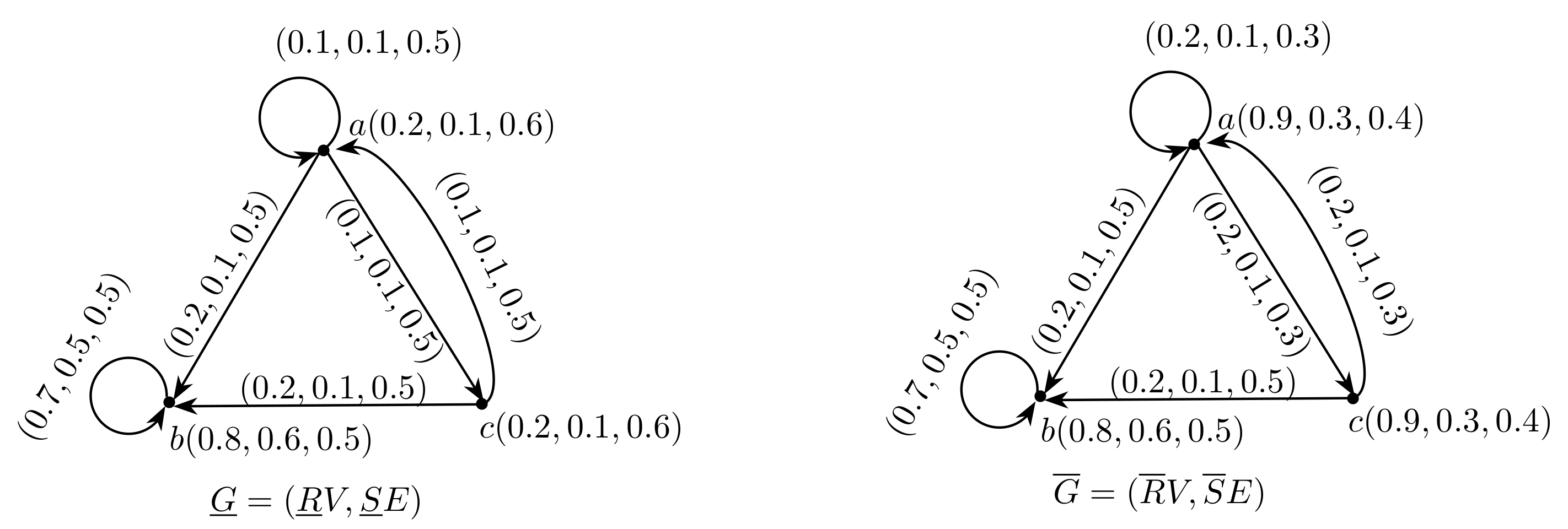
Example 1.
Let be a set and R an equivalence relation on
Let be a neutrosophic set on . The lower and upper approximations of V are given by,
Let and S an equivalence relation on defined as:
Let be a neutrosophic set on and a rough neutrosophic relation where and are given as
Thus, and are neutrosophic digraphs as shown in Figure 1.
We now form new rough neutrosophic digraphs from old ones.
Definition 6.
Let and be two rough neutrosophic digraphs on a set . Then, the intersection of and is a rough neutrosophic digraph , where and are neutrosophic digraphs, respectively, such that
Example 2.
Theorem 1.
The intersection of two rough neutrosophic digraphs is a rough neutrosophic digraph.
Proof.
Let and be two rough neutrosophic digraphs. Let be the intersection of and , where and . To prove that is a rough neutrosophic digraph, it is enough to show that a nd are neutrosophic relation on and , respectively. First, we show that is a neutrosophic relation on .
Thus, from above it is clear that is a neutrosophic relation on .
Similarly, we can show that is a neutrosophic relation on . Hence, G is a rough neutrosophic digraph. ◻
Definition 7.
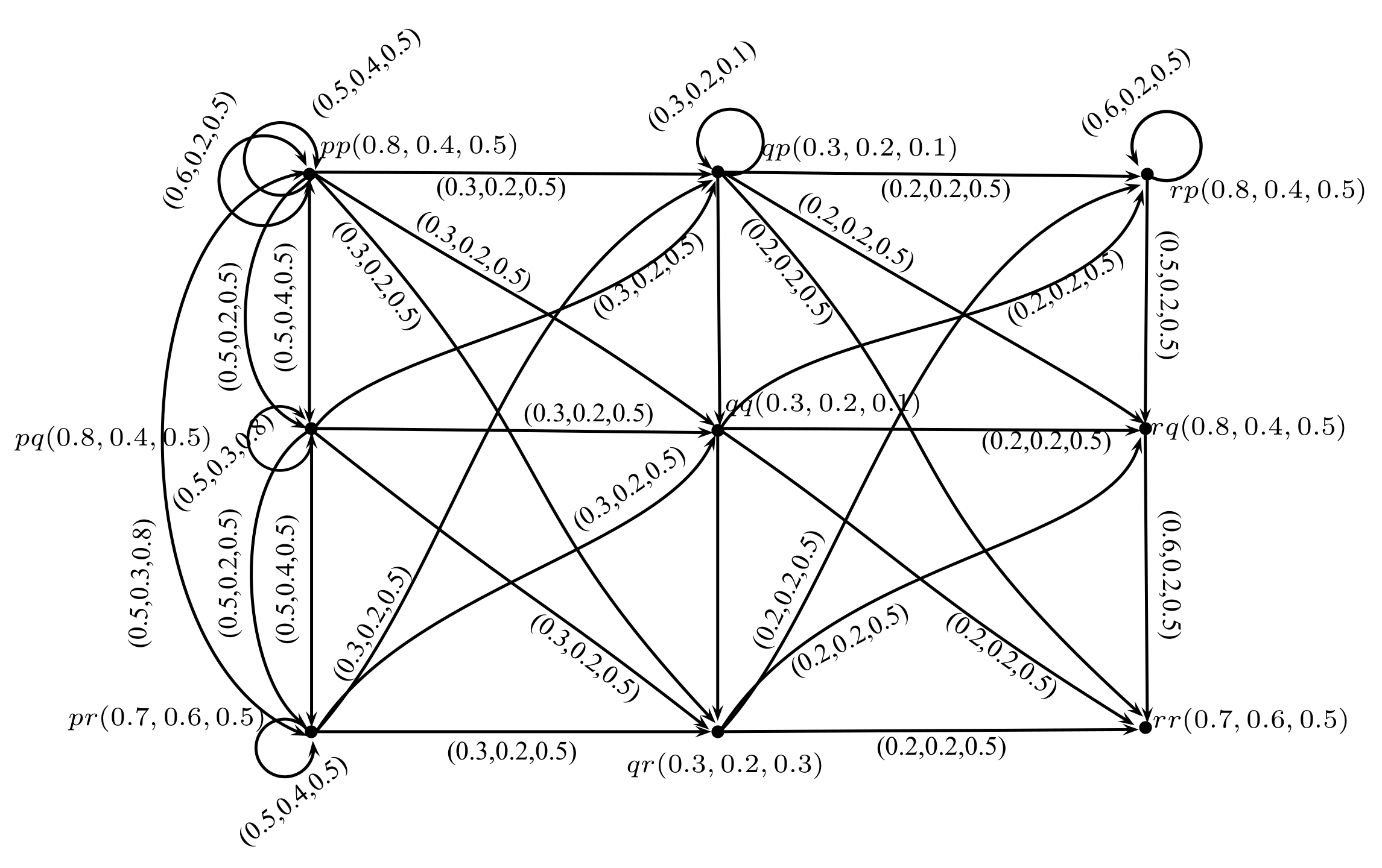
The Cartesian product of two neutrosophic digraphs and is a rough neutrosophic digraph , where and such that
Example 3.
Theorem 2.
The Cartesian product of two rough neutrosophic digraphs is a rough neutrosophic digraph.
Proof.
Let and be two rough neutrosophic digraphs. Let be the Cartesian product of and , where and . To prove that is a rough neutrosophic digraph, it is enough to show that and are neutrosophic relation on and , respectively. First, we show that is a neutrosophic relation on .
If , then
If , then
Thus, from above, it is clear that is a neutrosophic relation on .
Similarly, we can show that is a neutrosophic relation on . Hence, is a rough neutrosophic digraph. ◻
Definition 8.
The composition of two rough neutrosophic digraphs and is a rough neutrosophic digraph , where and are neutrosophic digraphs, respectively, such that
Example 4.
Theorem 3.
The Composition of two rough neutrosophic digraphs is a rough neutrosophic digraph.
Proof.
Let and be two rough neutrosophic digraphs. Let be the Composition of and , where and . To prove that is a rough neutrosophic digraph, it is enough to show that and are neutrosophic relations on and , respectively. First, we show that is a neutrosophic relation on .
If , then
If , then
If such that ,
Thus, from above, it is clear that is a neutrosophic relation on .
Similarly, we can show that is a neutrosophic relation on . Hence, is a rough neutrosophic digraph. ◻
Definition 9.
Let be a RND. The complement of G, denoted by is a rough neutrosophic digraph, where and are neutrosophic digraph such that
Example 5.
Consider a rough neutrosophic digraph as shown in Figure 4. The lower and upper approximations of graph G are and , respectively, where
The complement of G is . By calculations, we have
Thus, and are neutrosophic digraph, as shown in Figure 12.
Definition 10.
A rough neutrosophic digraph is self complementary if G and are isomorphic, that is, and .
Example 6.
Let be a set and R an equivalence relation on defined as:
Let be a neutrosophic set on . The lower and upper approximations of V are given as,
Let and S an equivalence relation on defined as
Let be a neutrosophic set on and a RNR where and are given as
Theorem 4.
Let be a self complementary rough neutrosophic digraph. Then,
Proof.
Let be a self complementary rough neutrosophic digraph. Then, there exist two isomorphisms and , respectively, such that
and
By Definition 7, we have
Similarly, it can be shown that
This completes the proof. ◻
3. Application
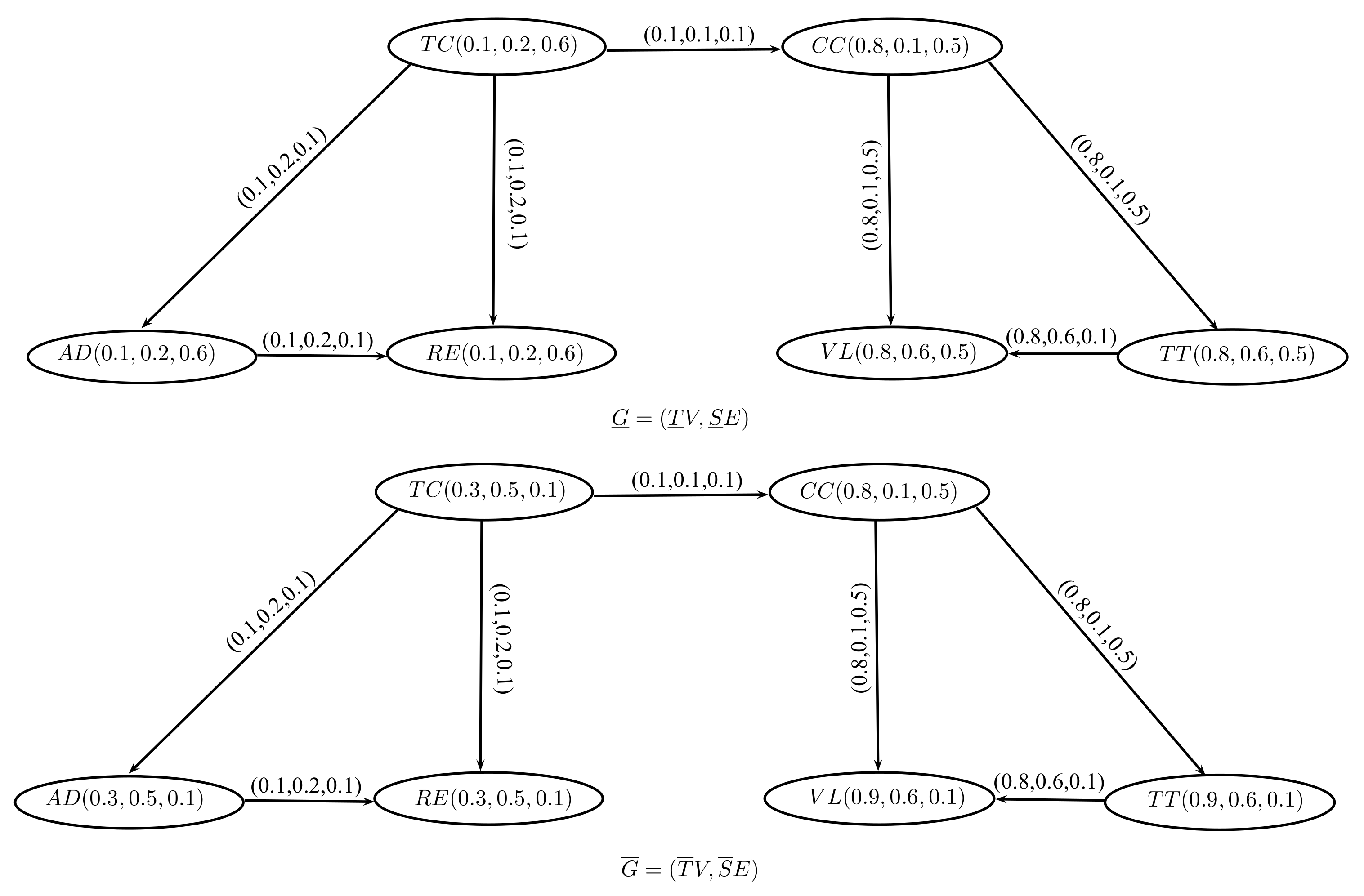
Investment is a very good way of getting profit and wisely invested money surely gives certain profit. The most important factors that influence individual investment decision are: company’s reputation, corporate earnings and price per share. In this application, we combine these factors into one factor, i.e. company’s status in industry, to describe overall performance of the company. Let us consider an individual Mr. Shahid who wants to invest his money. For this purpose, he considers some private companies, which are Telecommunication company (TC), Carpenter company (CC), Real Estate business (RE), Vehicle Leasing company (VL), Advertising company (AD), and Textile Testing company (TT). Let ={TC, CC, RE, VL, AD, TT} be a set. Let T be an equivalence relation defined on as follows:
Let be a neutrosophic set on with three components corresponding to each company, which represents its status in the industry and a rough neutrosophic set, where and are lower and upper approximations of V, respectively, as follows:
be the set of edges and S an equivalence relation on defined as follows:
be a neutrosophic set on which represents relationship between companies and a rough neutrosophic relation, where and are lower and upper upper approximations of E, respectively, as follows:
Thus, and is a rough neutrosophic digraph as shown in Figure 14.
To find out the most suitable investment company, we define the score values
where
and
of each selected company and industry decision is if By calculation, we have
, S(CC) = 1.4038, S(RE) = 0.0667, S(VL) = 0.3833, S(AD) = 0.1429 and S(TT) = 1.3529. Clearly, is the optimal decision. Therefore, the carpenter company is selected to get maximum possible profit. We present our proposed method as an algorithm. This Algorithm 1 returns the optimal solution for the investment problem.
| Algorithm 1 Calculation of Optimal decision |
|
4. Conclusions and Future Directions
Neutrosophic sets and rough sets are very important models to handle uncertainty from two different perspectives. A rough neutrosophic model is a hybrid model which is made by combining two mathematical models, namely, rough sets and neutrosophic sets. This hybrid model deals with soft computing and vagueness by using the lower and upper approximation spaces. A rough neutrosophic set model gives more precise results for decision-making problems as compared to neutrosophic set model. In this paper, we have introduced the notion of rough neutrosophic digraphs. This research work can be extended to: (1) rough bipolar neutrosophic soft graphs; (2) bipolar neutrosophic soft rough graphs; (3) interval-valued bipolar neutrosophic rough graphs; and (4) neutrosophic soft rough graphs.
Acknowledgments
The authors are very thankful to the Editor and referees for their valuable comments and suggestions for improving the paper.
Author Contributions
Sidra Sayed and Nabeela Ishfaq conceived and designed the experiments; Muhammad Akram performed the experiments; Florentin Smarandache contributed reagents/materials/analysis tools.
Conflicts of Interest
The authors declare that they have no conflict of interest regarding the publication of the research article.
References
- Smarandache, F. A Unifying Field in Logics. Neutrosophy: Neutrosophic Probability, Set and Logic; American Research Press: Rehoboth, NM, USA, 1999. [Google Scholar]
- Zadeh, L.A. Fuzzy sets. Inf. Control 1965, 8, 338–353. [Google Scholar] [CrossRef]
- Smarandache, F. Neutrosophy Neutrosophic Probability, Set, and Logic; American Research Press: Rehoboth, NM, USA, 1998. [Google Scholar]
- Wang, H.; Smarandache, F.; Zhang, Y.; Sunderraman, R. Single-valued neutrosophic sets. Multispace Multistructure 2010, 4, 410–413. [Google Scholar]
- Ye, J. Multicriteria decision-making method using the correlation coefficient under single-valued neutrosophic environment. Int. J. Gen. Syst. 2013, 42, 386–394. [Google Scholar] [CrossRef]
- Ye, J. Improved correlation coefficients of single valued neutrosophic sets and interval neutrosophic sets for multiple attribute decision making. J. Intell. Fuzzy Syst. 2014, 27, 2453–2462. [Google Scholar]
- Pawlak, Z. Rough sets. Int. J. Comput. Inf. Sci. 1982, 11, 341–356. [Google Scholar] [CrossRef]
- Dubois, D.; Prade, H. Rough fuzzy sets and fuzzy rough sets. Int. J. Gen. Syst. 1990, 17, 191–209. [Google Scholar] [CrossRef]
- Liu, P.; Chen, S.M. Group decision making based on Heronian aggregation operators of intuitionistic fuzzy numbers. IEEE Trans. Cybern. 2017, 47, 2514–2530. [Google Scholar] [CrossRef] [PubMed]
- Broumi, S.; Smarandache, F.; Dhar, M. Rough neutrosophic sets. Neutrosophic Sets Syst. 2014, 3, 62–67. [Google Scholar]
- Yang, H.L.; Zhang, C.L.; Guo, Z.L.; Liu, Y.L.; Liao, X. A hybrid model of single valued neutrosophic sets and rough sets: Single valued neutrosophic rough set model. Soft Comput. 2016, 21, 6253–6267. [Google Scholar] [CrossRef]
- Mordeson, J.N.; Peng, C.S. Operations on fuzzy graphs. Inf. Sci. 1994, 79, 159–170. [Google Scholar] [CrossRef]
- Akram, M.; Shahzadi, S. Neutrosophic soft graphs with applicatin. J. Intell. Fuzzy Syst. 2017, 32, 841–858. [Google Scholar] [CrossRef]
- Akram, M.; Sarwar, M. Novel multiple criteria decision making methods based on bipolar neutrosophic sets and bipolar neutrosophic graphs. Ital. J. Pure Appl. Math. 2017, 38, 368–389. [Google Scholar]
- Akram, M.; Siddique, S. Neutrosophic competition graphs with applications. J. Intell. Fuzzy Syst. 2017, 33, 921–935. [Google Scholar] [CrossRef]
- Akram, M.; Sitara, M. Interval-valued neutrosophic graph structures. Punjab Univ. J. Math. 2018, 50, 113–137. [Google Scholar]
- Zafer, F.; Akram, M. A novel decision-making method based on rough fuzzy information. Int. J. Fuzzy Syst. 2017. [Google Scholar] [CrossRef]
- Banerjee, M.; Pal, S.K. Roughness of a fuzzy set. Inf. Sci. 1996, 93, 235–246. [Google Scholar] [CrossRef]
- Liu, P.; Chen, S.M.; Junlin, L. Some intuitionistic fuzzy interaction partitioned Bonferroni mean operators and their application to multi-attribute group decision making. Inf. Sci. 2017, 411, 98–121. [Google Scholar] [CrossRef]
- Liu, P. Multiple attribute group decision making method based on interval-valued intuitionistic fuzzy power Heronian aggregation operators. Comput. Ind. Eng. 2017, 108, 199–212. [Google Scholar] [CrossRef]
- Zhang, X.; Dai, J.; Yu, Y. On the union and intersection operations of rough sets based on various approximation spaces. Inf. Sci. 2015, 292, 214–229. [Google Scholar] [CrossRef]
- Bao, Y.L.; Yang, H.L. On single valued neutrosophic refined rough set model and its application. J. Intell. Fuzzy Syst. 2017, 33, 1235–1248. [Google Scholar] [CrossRef]
Figure 1.
Rough neutrosophic digraph .

Figure 2.
Rough neutrosophic digraph .

Figure 3.
Rough neutrosophic digraph .

Figure 4.
Rough neutrosophic digraph .
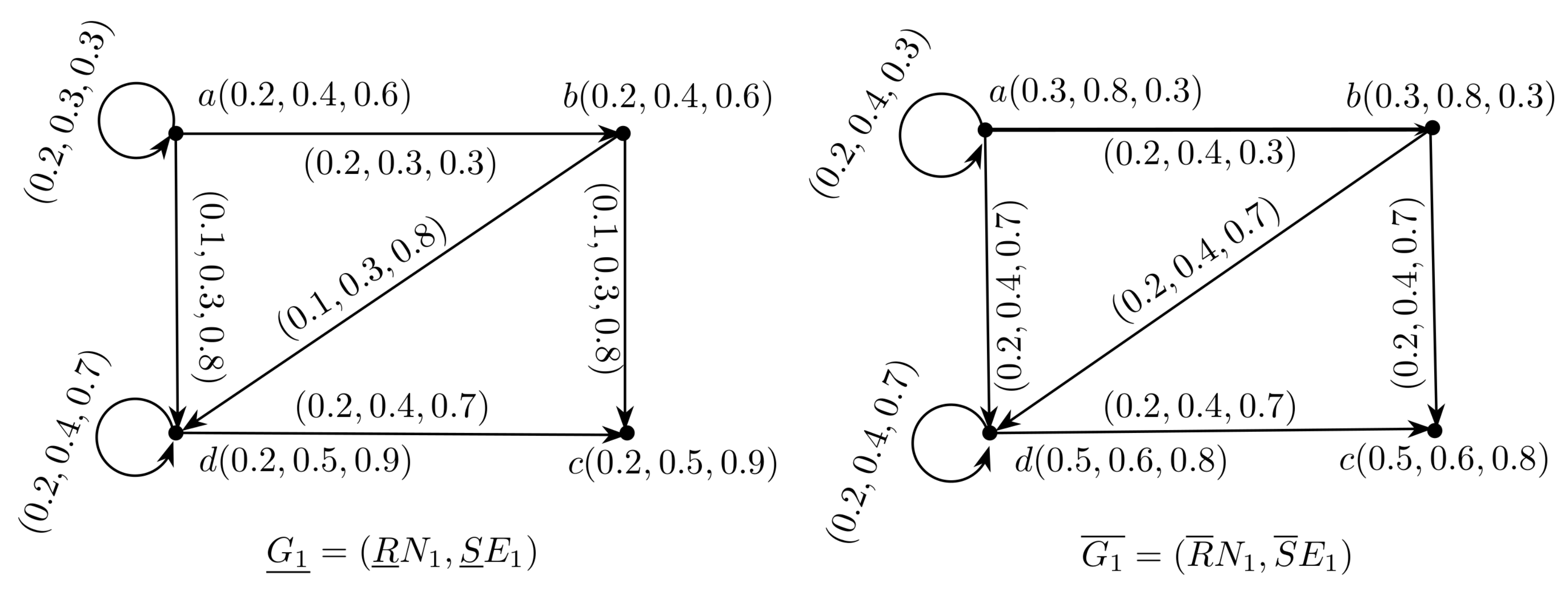
Figure 5.
Rough neutrosophic digraph .
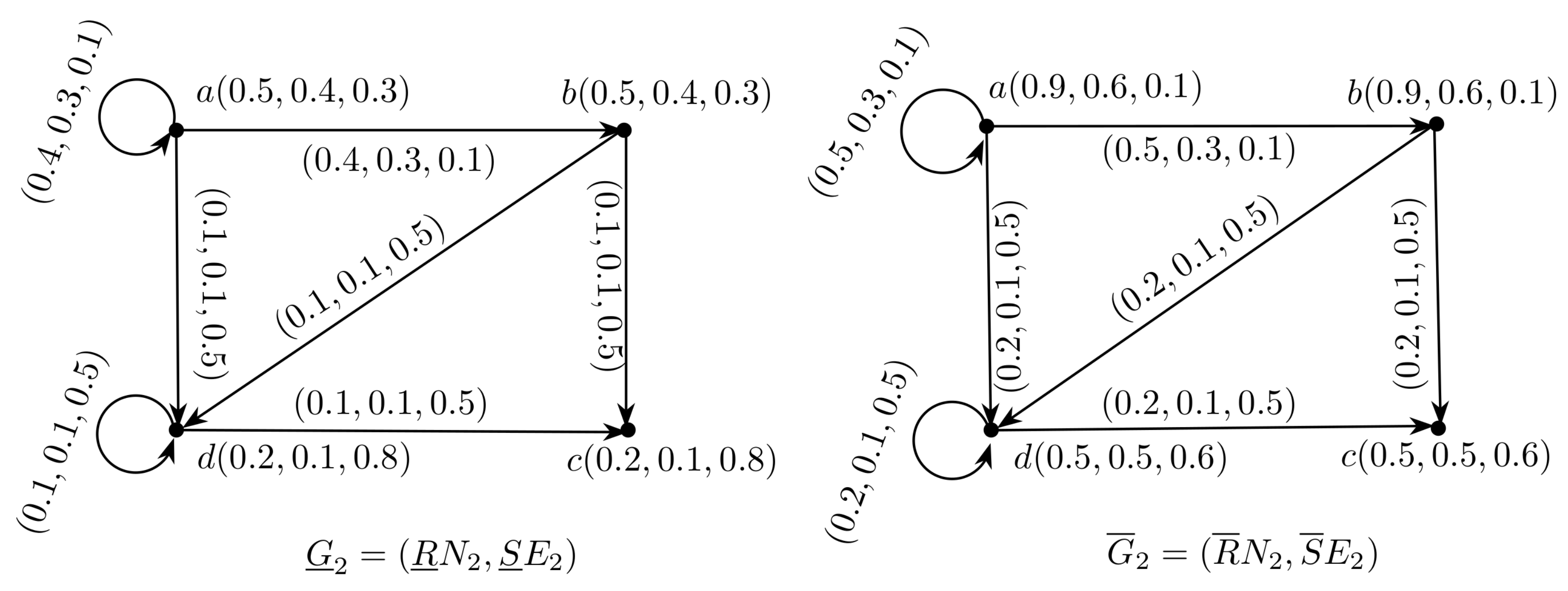
Figure 6.
Neutrosophic digraph .
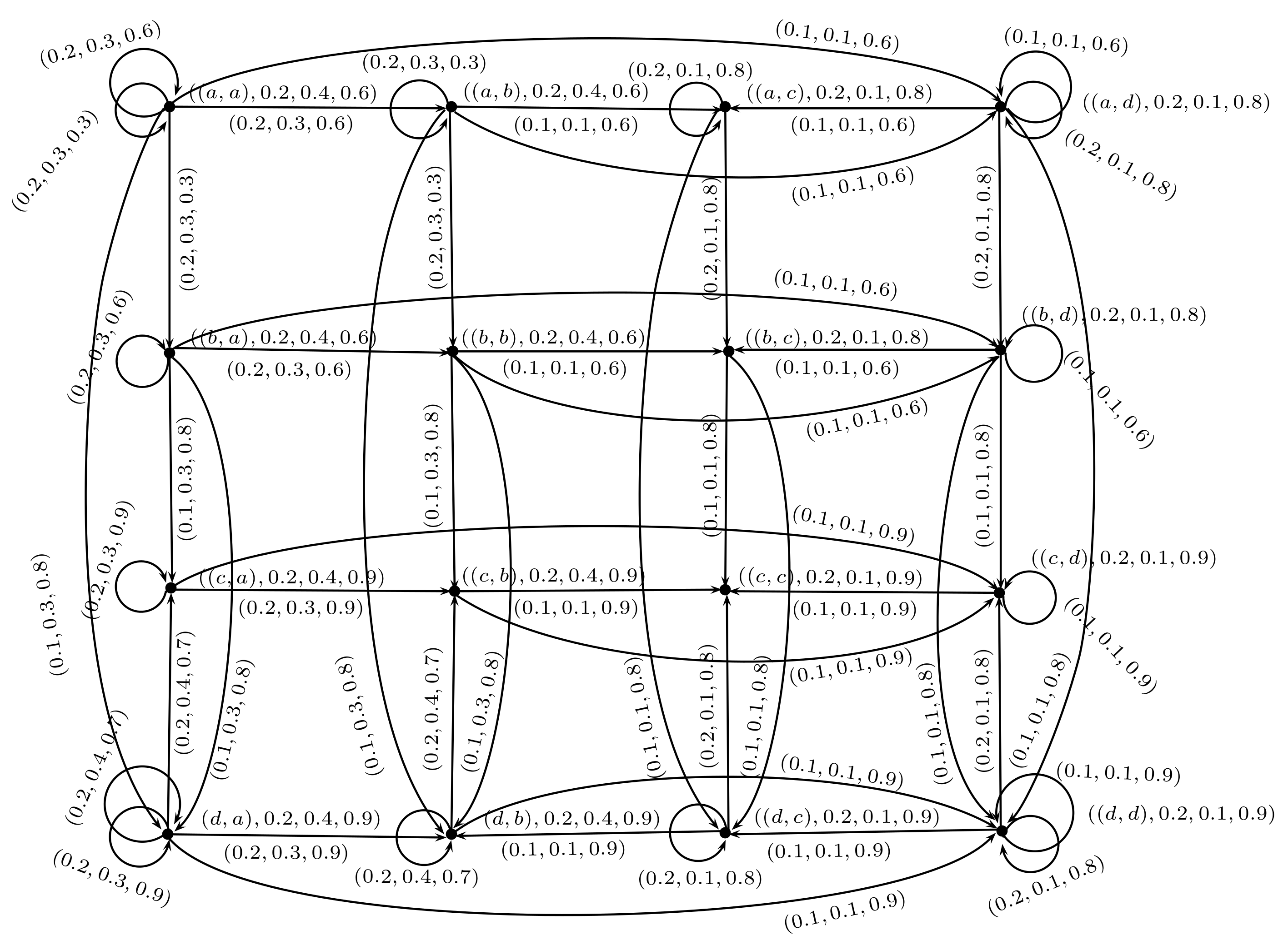
Figure 7.
Neutrosophic digraph .
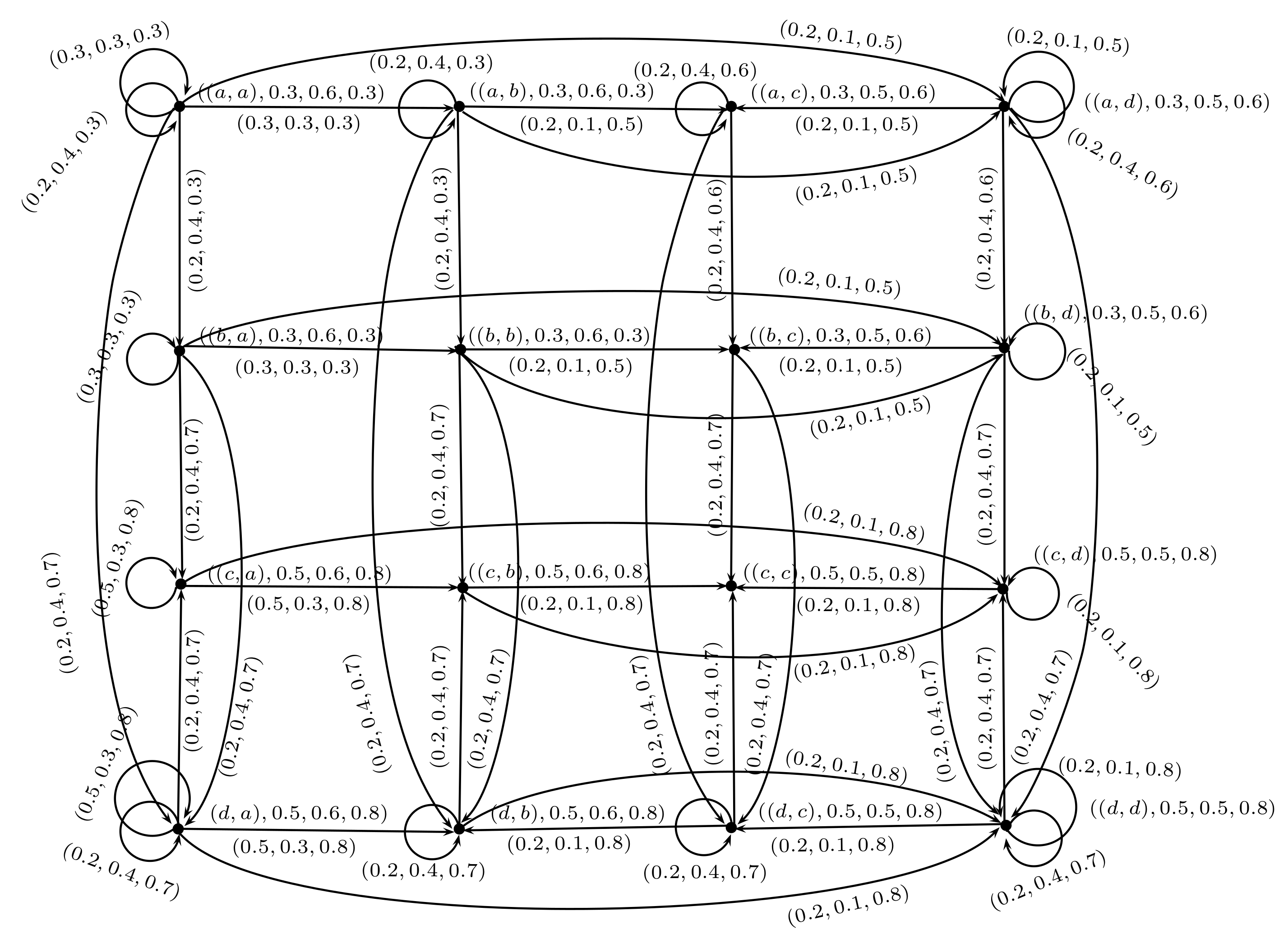
Figure 8.
Rough neutrosophic digraph .

Figure 9.
Rough neutrosophic digraph .
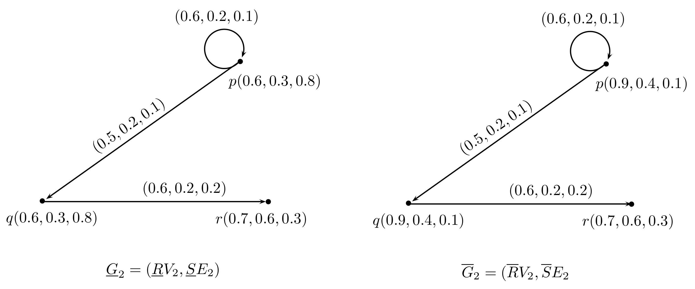
Figure 10.
Neutrosophic digraph .
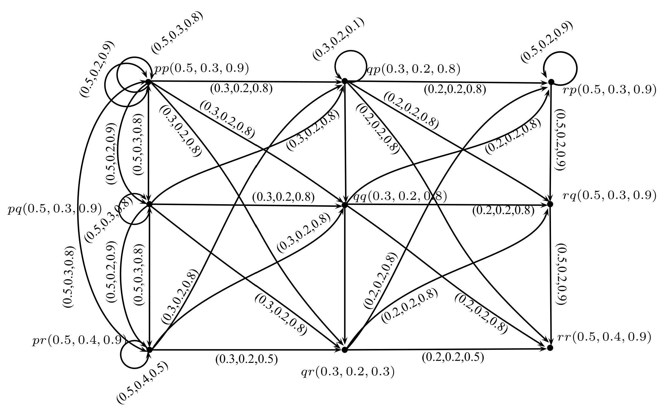
Figure 11.
Neutrosophic digraph .

Figure 12.
Rough neutrosophic digraph .
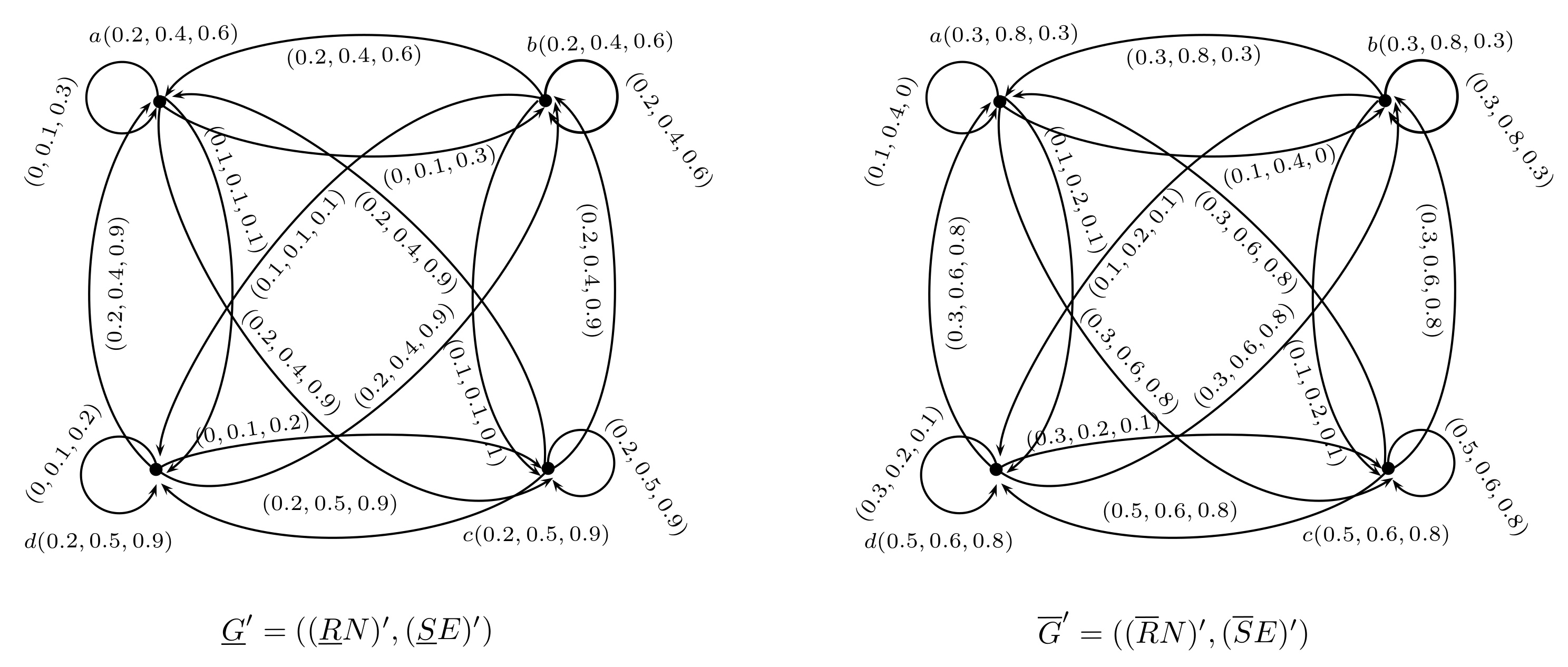
Figure 13.
Self complementary RND .
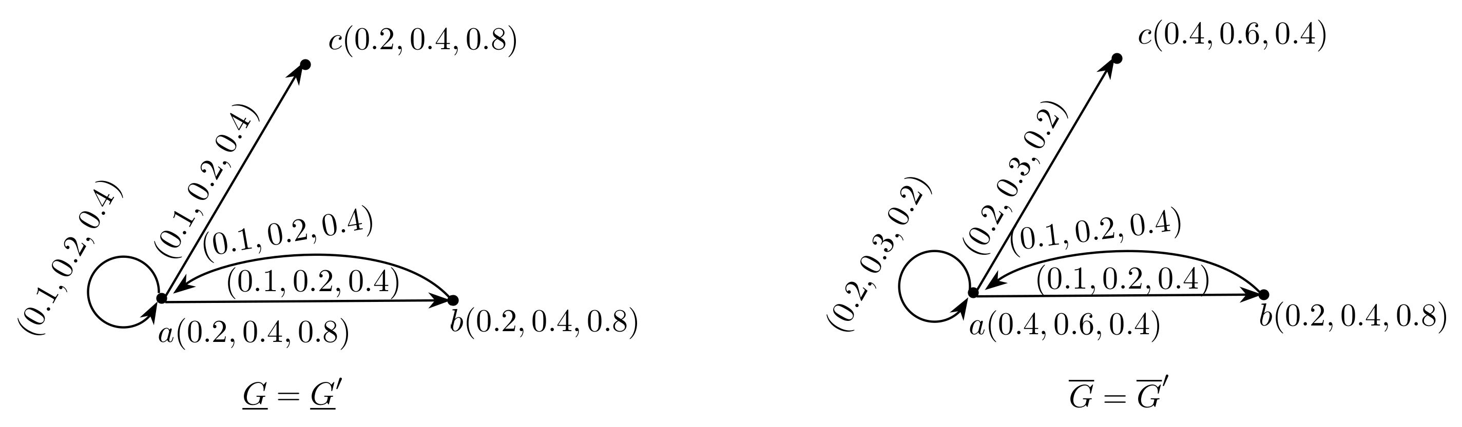
Figure 14.
Rough neutrosophic digraph .

© 2018 by the authors. Licensee MDPI, Basel, Switzerland. This article is an open access article distributed under the terms and conditions of the Creative Commons Attribution (CC BY) license (http://creativecommons.org/licenses/by/4.0/).
Share and Cite
MDPI and ACS Style
Sayed, S.; Ishfaq, N.; Akram, M.; Smarandache, F. Rough Neutrosophic Digraphs with Application. Axioms 2018, 7, 5. https://doi.org/10.3390/axioms7010005
AMA Style
Sayed S, Ishfaq N, Akram M, Smarandache F. Rough Neutrosophic Digraphs with Application. Axioms. 2018; 7(1):5. https://doi.org/10.3390/axioms7010005
Chicago/Turabian StyleSayed, Sidra, Nabeela Ishfaq, Muhammad Akram, and Florentin Smarandache. 2018. "Rough Neutrosophic Digraphs with Application" Axioms 7, no. 1: 5. https://doi.org/10.3390/axioms7010005
Note that from the first issue of 2016, this journal uses article numbers instead of page numbers. See further details here.