Self-Sensing Electromagnets for Robotic Tooling Systems: Combining Sensor and Actuator

Abstract

A low-cost method, which integrates distance sensing functionality into a switched electromagnet by using a hybrid switching mode and current ripple measurements, is proposed. The electromagnet is controlled by a micro-controller via a MOSFET H bridge, utilizing a comparator-based current control. Additionally, a method for calculating the inductance of the electromagnet and approximating the magnetic contact between the electromagnet and its target is also presented. The resulting tool is attached to an industrial robot, and the system performance using this setup is evaluated. Distance sensing in the range of 0 mm to 5.2 mm is demonstrated. It is also shown that the relation between magnetic contact, coil current and calculated inductance can be reduced to a predictive look-up table, enabling the quality of the magnetic contact to be estimated using minimal computational effort.

1. Introduction

Electromagnets are commonly used within the field of industrial robotics. They are often mounted on robotic tools used to lift ferromagnetic materials, such as steel sheets or scrap metal. Another commonly-used industrial component is the inductive proximity sensor, used to detect if any metallic object is in close proximity to the sensor. These two components are sometimes used together and sometimes as parts of robotic tools, where the sensor is used to detect the object which the electromagnet then will lift. This setup gives the combined tool a distinct advantage over a similar, but sensor-less tool in that it can compensate for changes in its environment. It can for example be used to compensate for individual tolerances when working with a large number of objects [1].

This article will demonstrate a setup that combines the lifting functionality of the electromagnet with the proximity sensing functionality of the inductive proximity sensor. The setup may be referred to as a “self-sensing” electromagnet, able to not only create a lifting force, but also to detect the proximity of any ferromagnetic object. This is of interest for applications where space is limited, where the electromagnet blocks the whole surface of interest or when having a comparably sensitive inductive sensor paired with an electromagnet is unsuitable, such as in heavy duty equipment. Another advantage is that a separate sensor does not need to be installed, potentially reducing system cost, but the trade-off is that the control electronics become more complex.

An additional benefit of this setup is the ability to control the currents in the electromagnets, giving the option of force control. This can be of interest for applications where controlling the force during the lift could be beneficial, such as lifting a stack of thin steel sheets [2]. Similar concepts regarding self-sensing electromagnets have been explored in the field of magnetic levitation, see, e.g., [3,4,5,6]. Another proposed application is active vibration dampening of mechanical parts [7], such as steel sheets in a metalworking rolling-press [8]. Self-sensing systems have also been used to estimate the rotor position and rotational speed of electric motors [9,10].

The system presented here is a part of the ongoing wave-power research project at Uppsala University [11]. The aim of this specific project is to further develop the production technology needed to mass-produce wave-power generator units while keeping implementation costs down. The robotic tool presented here is used to locate and mount steel plates used in the translator of the generator, an application requiring around 1 $\mathrm{k}\mathrm{N}$ of force and 0.1 mm positional accuracy.

To highlight the difference between a “normal” inductive sensor and the setup presented in this paper, one must first know the principle behind the first one. In a normal “commercial grade” inductive proximity sensor, a magnetic field is generated by the use of an LC-resonance circuit with frequencies in the kHz or MHz band, where the core of the inductance is exposed to the outer world. If any object disturbs this magnetic field, this will affect the inductance and in turn the frequency and amplitude of the resonance signal [12]. This change is often picked up directly by an electronic circuit monitoring the voltage in the LC-circuit, but designs using a secondary pickup-coil that reacts on changes in the magnetic field also exists.

The setup presented here uses none of the above approaches due to the following reasons. Firstly, a normal LC-resonance circuit oscillates around a zero voltage and current level, with an average value of zero. This would not work in this system as the current needs to have a DC-bias in order to generate an approximately constant magnetic field, used to generate the lifting force. This leaves us with the alternative of using a separate pickup-coil. A setup would work even with a DC-bias on the current, but it would require modifying the standard electromagnets in order to insert this extra coil. A modification of the electromagnets was not desirable, since a goal of the project was the ability to use a standard off-the-shelf component, in order to keep costs down.

The presented measurement system is instead based on the idea of current ripple measurements [13]. The principal idea is here that when an inductive load, such as an electromagnet, is controlled using a switching circuit, the frequency and amplitude of the current ripple contain information about the state of the system as a whole. Accessing this information then only requires the current ripple to be correctly analyzed. The most interesting property to extract in this case is the inductance of the electromagnet, as it is directly coupled to the length of the air-gap between the electromagnet and its target.

However, while this idea is theoretically sound, its practical implementation has proven to be challenging [14]. Switched current control systems are in general designed to have as low a current ripple as possible, making the actual current ripple measurements more challenging, often requiring expensive high-accuracy measurement equipment.

Here, a different approach is proposed, not requiring high accuracy components, thus reducing cost. The main idea of this new approach is to perform the current ripple measurement on a single, much larger, temporary current pulse instead of the normal, comparably small, current ripple. This larger pulse can be introduced as either a step in the current reference or as a temporary lock-up of the driving switches.

If done correctly, this will result in a single larger pulse in the current. The relevant measurements are then performed on this pulse. However, if the pulse is made too big, it will disrupt the normal operation of the system, and if it is too small, nothing will be gained with regards to measurement accuracy. Therefore, a balance has to be found between the two.

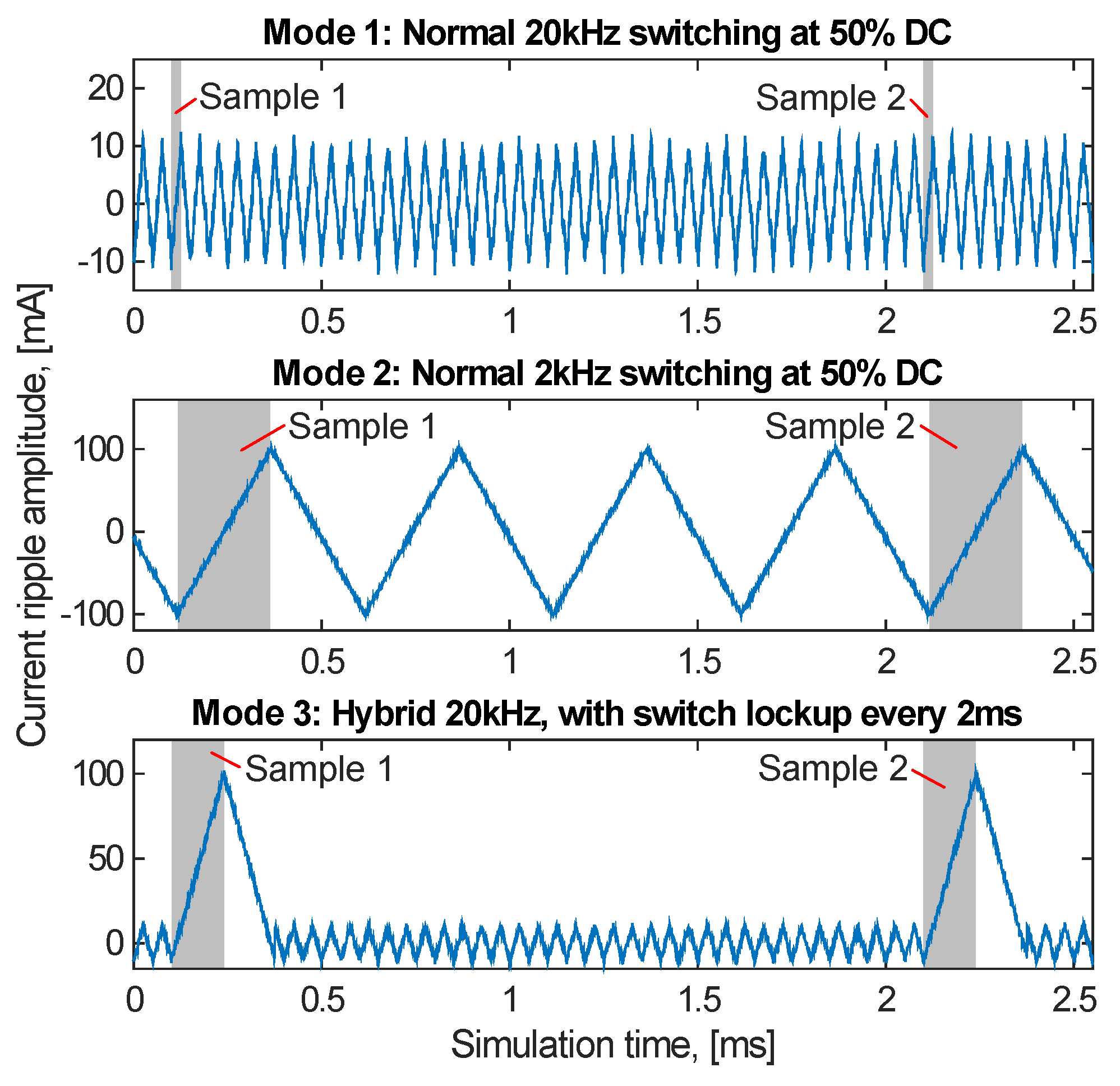
To illustrate the principle of this approach, consider the following case: The rise-time of the current in a switched ideal electromagnet is to be sampled at 500 Hz. The nominal switching frequency of the electromagnet can be set to either 20 kHz or 2 kHz, giving a corresponding current ripple of either 10 mA or 100 mA, respectively. A third “hybrid” mode of operation is also available, where the nominal switching frequency is set to 20 kHz, but with the added option to temporarily lock the switches every 2 ms. The current measurement system is assumed to have a randomly distributed noise with a maximum amplitude of 2.5 mA. See Figure 1 and

Table 1. Comparison of switched operation modes.

	Mode 1	Mode 2	Mode 3
SNR (RMS quota)	12.3 dB	32.1 dB	26.0 dB
RMS current	5.94 $\mathrm{m}\mathrm{A}$	57.8 $\mathrm{m}\mathrm{A}$	21.2 $\mathrm{m}\mathrm{A}$
Audible noise	None	2 kHz	500 Hz
Acquisition time	25 μs	250 μs	140 μs

, where Mode 3 is the case of interest.

In summary, it can be said that the motivation for implementing this new system is that Mode 3 offers a Signal to Noise Ratio (SNR) around 4.8-times better than that of Mode 1. The main drawback for this increase in SNR is that the acquisition time increases with 115 μs and that the RMS current ripple rises with 15.26 mA, compared to Mode 1, but it remains lower than the RMS current for Mode 2. Another, more subjective advantage, is the ability to tailor the audible noise to a, for humans, more pleasant tone. This, as the constant kilohertz noise from Mode 2, can be perceived as annoying in an industrial environment. Using this method, the induced 500 Hz noise can be lowered to, for example 50 Hz or even sub-audible frequencies, if the application allows for such a relatively slow sampling rate.

The system was realized using an electromagnetic tool mounted on an industrial robot. The electromagnet was then controlled using an MCU-controlled MOSFET H bridge. The MCU was also used to collect and process relevant measurement data. Using these data and electromagnetic theory, a relation between the air-gap and the measured current rise-times could be constructed.

2. Method

2.1. Experimental Setup

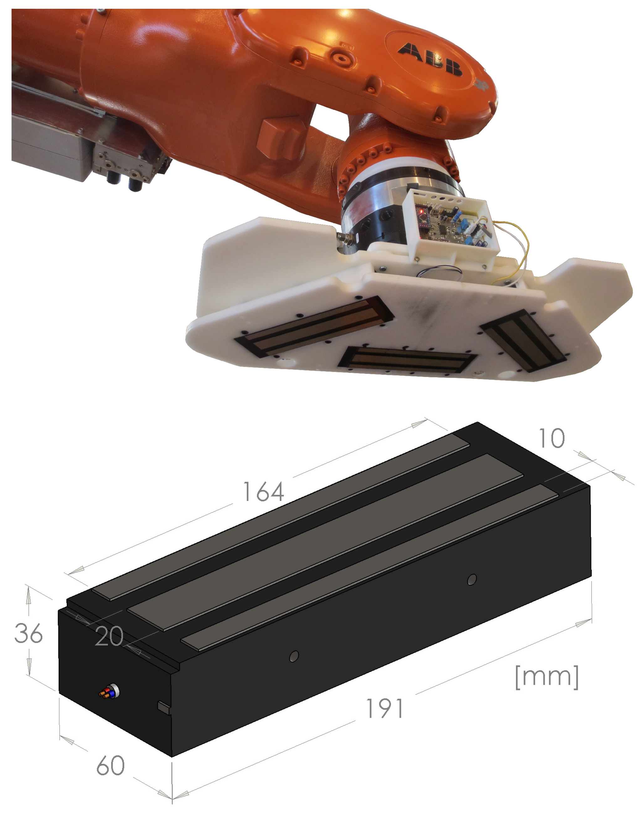
The setup consisted of a floor-mounted industrial robot, ABB IRB-6650S, with a prototype electromagnetic tool mounted on the end of the robotic arm. The usage of a robotic arm allowed for precise movements of the mounted tool and also high repeatability of said movements; see Figure 2.

The robotic tool consisted of three electromagnets, a plastic support structure and the Current Control Board (CCB). The CCB regulated and measured the current flowing through the three electromagnets, which were connected in parallel. The system was powered by the built-in 24 $V_{dc}$ supply of the robot. Communication with the CCB was achieved using a wired serial-data interface.

A flat and uniform plate of DOMEX 355 MC steel, 15 mm thick, was used as the target for the electromagnets during the experiments, unless otherwise stated.

2.1.1. Current Control Board

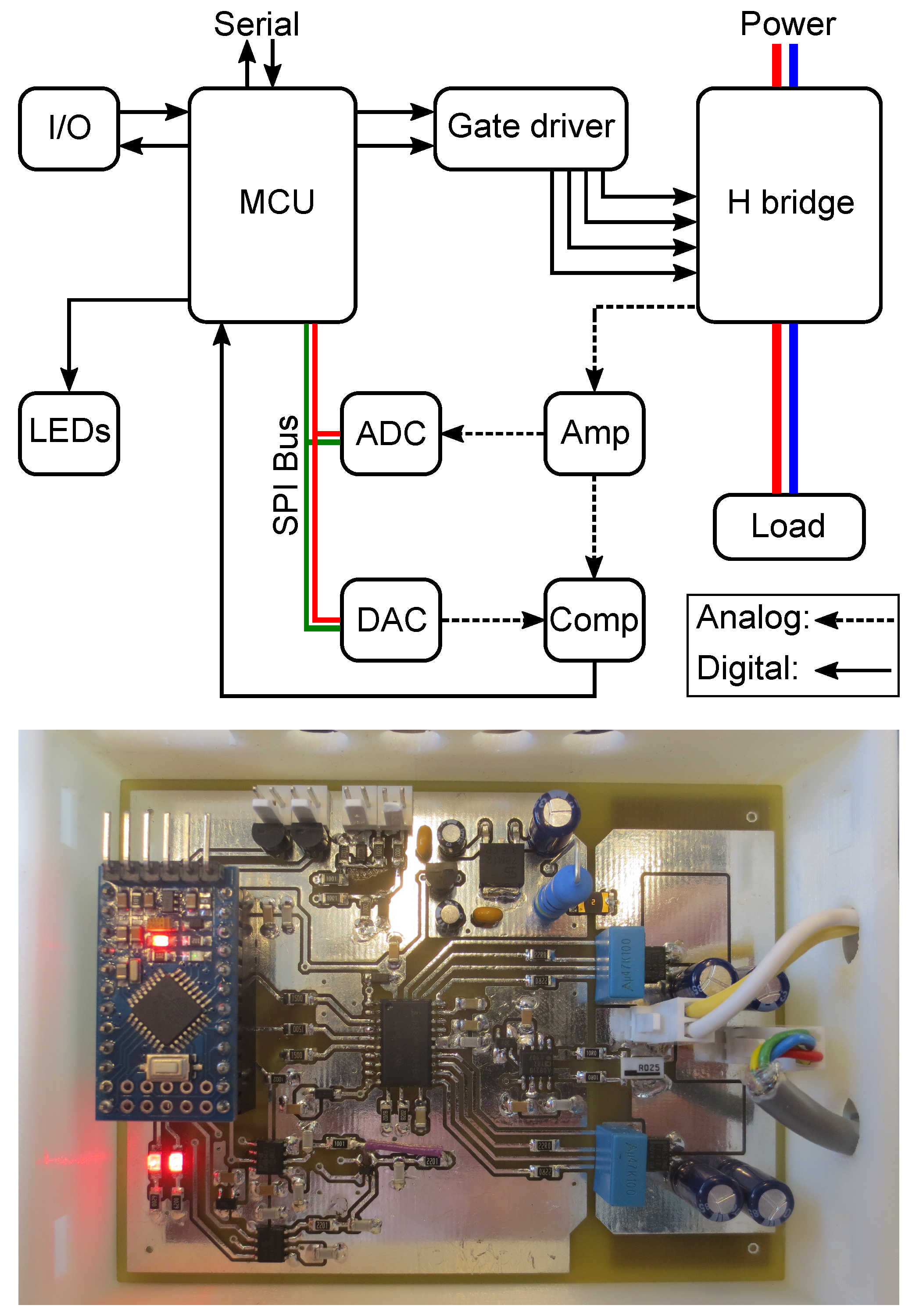
The CCB consisted of four MOSFETs (CSD88537ND) in an H bridge configuration. The MOSFETs were controlled by a micro-controller (MCU-ATMEGA328P) through a gate driver IC (Integrated Circuit) (HIP4080A). Current measurements were performed using a shunt resistor and a shunt current monitor (AD8210). The output from the monitor was in turn connected to two devices. The first was an ADC (MCP3201), which allowed the MCU to read the current measurement as a binary code; the second was the inverting pin of a comparator (TLV3201). The non-inverting pin of the comparator was connected to a DAC (MCP4921) controlled by the MCU. The comparator output was in turn connected to an interrupt capable I/O pin on the MCU. See Figure 3 for a schematic representation of the CCB.

This setup allowed the comparator to trigger each time the difference between the ADC-input and the DAC-output changed polarity, something that was used to control the timing of the measurements. A picture of the CCB is shown in Figure 3, and general specifications can be seen in

Table 2. General CCB specifications.

Parameter	Value
Current capability	±5 $\mathrm{A}$
Supply voltage	15–35 $V_{dc}$
MCU clock	16 MHz
Serial link speed	38.4 $\mathrm{k}$bit$·$s${}^{-1}$
Switching frequency	0–80 kHz
Component price	∼20 USD

. For simplicity, the current control was implemented as a bang bang control using the comparator and current sense amplifier on the CCB with a 5 $\mathrm{m}\mathrm{A}$ hysteresis band around the current DAC value.

2.1.2. Electromagnets

The electromagnets (see Figure 2) were designed to operate at 24 $V_{dc}$ and had an internal resistance of approximately 24.2 Ω, effectively limiting the current to around 990 $\mathrm{m}\mathrm{A}$. In total, three electromagnets were connected to the CCB in parallel with a maximal DC current drain of just under 3 $\mathrm{A}$, well within the specifications of the CCB. Note that each of the three electromagnets was originally designed to be used as automatic door locks. While the iron core was laminated using 0.6 $\mathrm{m}\mathrm{m}$ thick laminates, the original control circuitry probably did not use a switched control method and instead relied on linear voltage regulation. Using these electromagnets in a switched environment therefore meant taking them outside their normal operating range. Each electromagnet had a specified static holding force of 650 $\mathrm{k}\mathrm{g}$ at rated current.

2.1.3. Communication

The CCB used an ASCII-based serial data communication protocol. The serial data stream, containing system measurements, was sent from the CCB to an external PC acting as the system master. A MATLAB script running on the master PC was used to log and process the data. This script also allowed for sending new settings and reference values to the CCB.

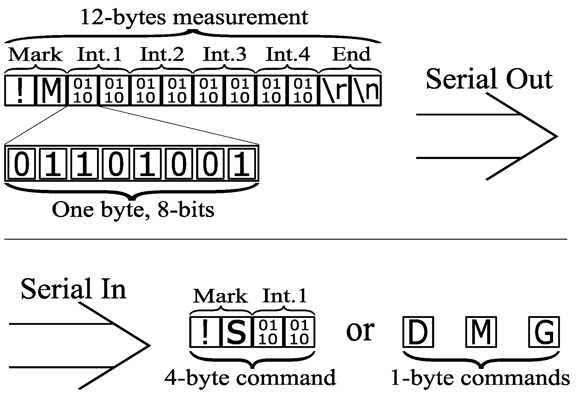
In order to save transmission time, the measurement data from the CCB was sent as a 12-byte binary package as opposed to individual ASCII symbols; see Figure 4. This as a 16-bit binary number can be as long as five characters long, with each ASCII character taking up 1 byte, for a total of five bytes per measurement point. The first two bytes in each package were used as an identifier, containing two ASCII characters. The next eight bytes were used for storing binary data. These eight bytes were in turn divided into four 16-bit unsigned integers (uint16) for a total of four possible data-points in each package. The last two bytes were used for new-line and carriage-return characters. This approach reduced the size of each measurement from 24 bytes (2 bytes start + four times 5 bytes of ASCII characters + 2 bytes end) to 12 bytes (2 bytes start + four times 2 bytes of unsigned integers + 2 bytes end).

Data sent to the MCU were sent as either 1-byte single ASCII character commands or as 4-byte binary code containing two identifier ASCII characters followed by one 16-bit integer.

2.2. CCB Measurement Implementation

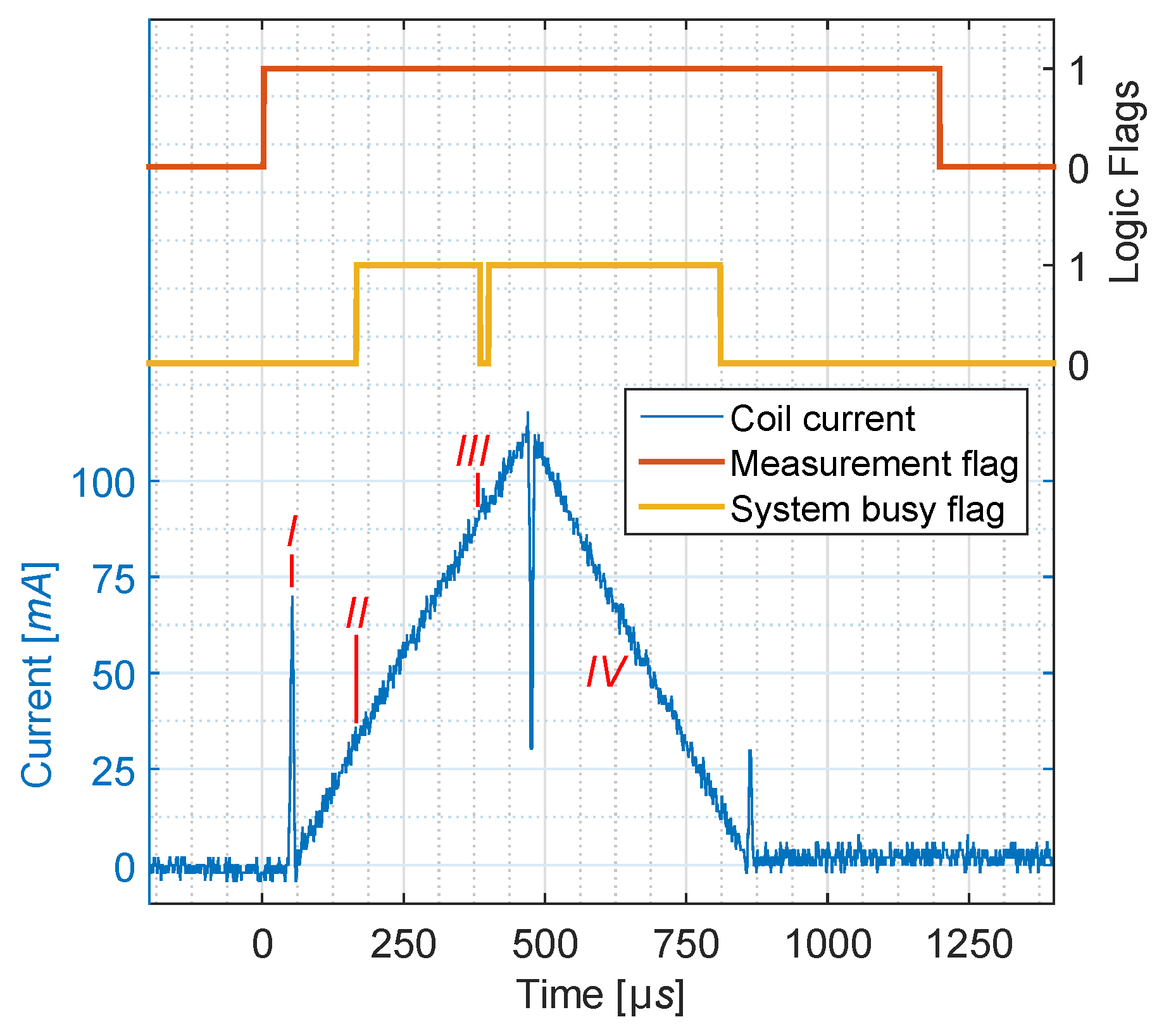
The measurement system measured three parameters of the current ripple: initial current, final-current and the time to change between them, here called rise-time. The routine was programmed onto the MCU and utilized the available DAC, ADC and comparator. The measurement process itself was divided into four separate steps; see Figure 5. Each step is individually described below (values are taken from Figure 5 as an example).

• Step I:
  When a measurement is requested, either by a serial command or system time-out, Step I of the measurement cycle is triggered. This prepares the system for taking a measurement. This is done by putting an internal measurement flag of the MCU high and then detecting in what direction the current step is supposed to happen, determined by whether the current reference is positive or negative. The MOSFETs are then locked in such a configuration that the current rises in the desired direction. Additionally, the DAC reference value is offset from the nominal current reference in order to shift the comparator trigger level to a point above or below the current value, depending on the current step direction. In this case, 15 $\mathrm{m}\mathrm{V}$ above nominal, corresponding to approximately 32 $\mathrm{m}\mathrm{A}$.
• Step II:
  When the current measurement has risen to the new offset value of the DAC, detected by a change of the comparator output, Step II is triggered as an Interrupt Service Routine (ISR) on the MCU. This causes the measurement to begin with a reset of the system clock register to zero and then taking a measurement of the current. This measurement is saved as the initial current, $i_{start}$. Additionally, the system is flagged as busy, so that the measurement timing is not disturbed by any other process. Finally, the DAC value is once again offset in the same direction as in Step I, but this time by a larger amount. Here, 40 $\mathrm{m}\mathrm{V}$ above the normal level, corresponding to approximately 87 $\mathrm{m}\mathrm{A}$.
• Step III:
  Triggered when the current has once again reached the DAC offset and the comparator again changes state, another ISR is started. First, the value of the system clock register is saved as the rise-time, $t_r$, followed by a measurement of the final current, $i_{end}$. Additionally, the DAC value and busy flag are reset, and the MOSFET states are unlocked so that the control system can control them once more. This marks the end of the data collection part of the measurement.
• Step IV:
  Detecting the change of state of the busy flag, the control system takes back the control of the MOSFETs and starts to force down the current towards its default level. While the current is decreasing, the system is once more flagged as busy as the measurement data are processed and filtered. If the CCB is connected to a host that is accepting serial data, this would also be the time for the data transmission. Once the filter is updated, the busy flag is reset, and after both the busy flag and serial transmission are done, the measurement flag is reset, as well. After this, the system goes back to normal operation. The system will remain in Step IV until the next measurement is requested and the cycle repeats.

Filtering of the step time was done by implementing a 6th order, 64-bit integer digital Butterworth-filter directly into the MCU on the CCB using a “direct-form II transposed” implementation with pre-calculated coefficients. It takes around 412 μs for the MCU to update the filter after each measurement, as can be seen from the busy flag in Figure 5.

2.3. Calculating Inductance from Rise-Time

Using the previously-obtained rise-time and current measurement, the inductance of the system can be calculated. Knowing the inductance is of interest for two reasons:

Firstly, due to the relatively low permeability of air, the inductance of the electromagnets becomes strongly coupled to the length of the air-gap between the electromagnet and its target, where a larger air-gap leads to lower inductance. Knowing this relation allows for the use of the electromagnet as a distance sensor, as each value of the inductance corresponds to a certain air-gap.

Secondly, the grade of magnetic contact in the air-gap can be evaluated by observing the change in inductance for different currents. This can, in turn, be used to evaluate if the electromagnet has successfully connected to its intended target or not, something that can be used to optimize industrial processes.

Finding an accurate inductance model for these electromagnets proved challenging. As demonstrated in [15], even for a well-specified geometry, the inductance model for the switched (AC) case for a laminated core depends on numerous variables, e.g., the electrical resistivity of the laminates and wire, the number of turns and layers in the coil, parasitic capacitances and winding pitch. In this setup, this becomes even worse, as there is a mix of both laminated and non-laminated steel in the magnetic circuit. This led to the conclusion that the electromagnets were to be considered as “black-boxes” and as such desired parameters and system responses had to be measured, rather than modeled as basically everything besides lamination thickness and coil resistance was unknown.

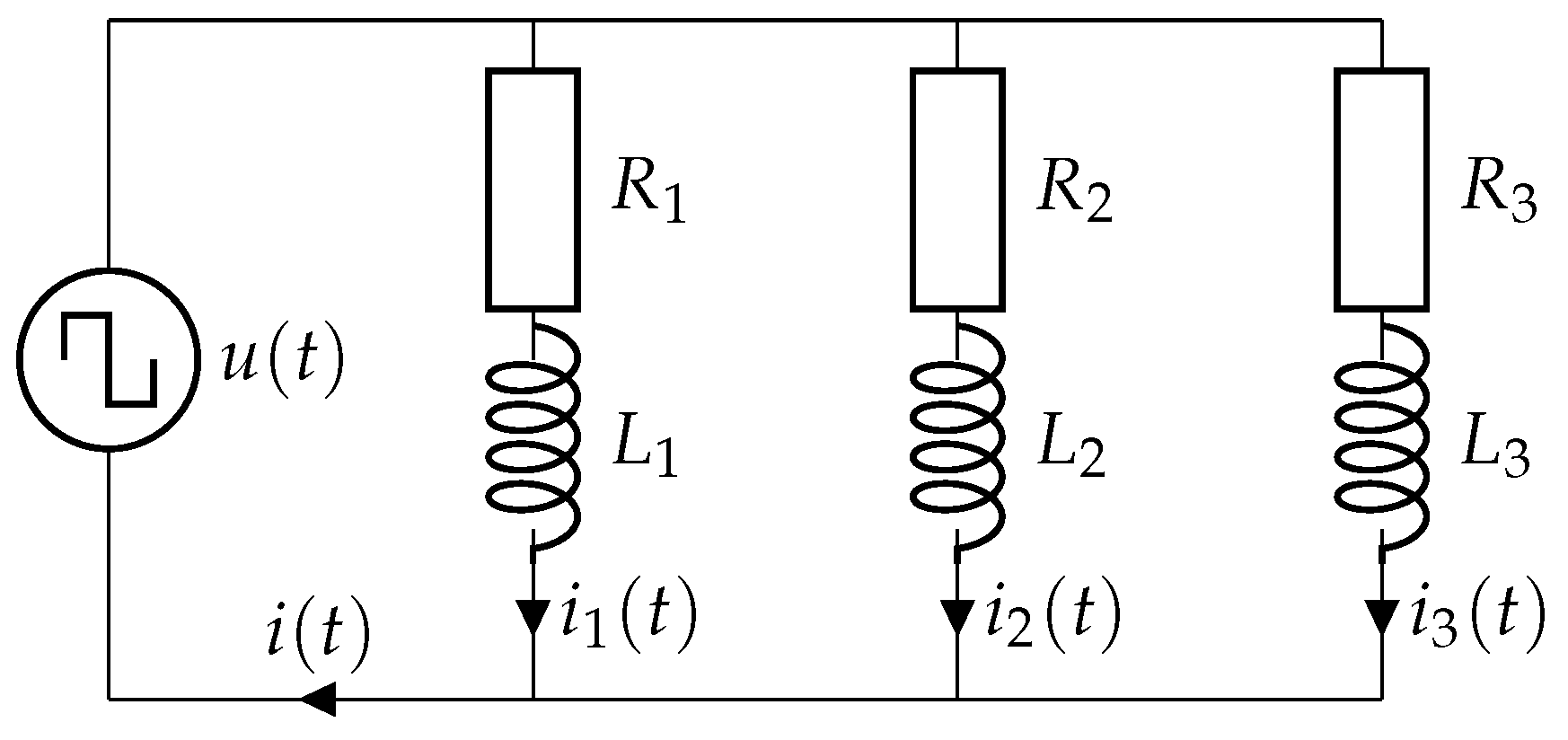
An RL (Resistor-Inductor) model of the electromagnet could, however, be used to derive a simplified analytical model of the electromagnet, despite the many unknown parameters; see Figure 6. Note that as this system will sometimes evaluate the inductance between two non-zero bias currents, so are the formulas adapted to calculate the dynamic inductance and not the “normal” static inductance, as explained by [16] among others.

Using basic circuit theory, this model can be described by the following relations:

$$u\left(t\right)=R_n{i}_n\left(t\right)+L_n\frac{d{i}_n\left(t\right)}{dt}\{n=1,2,3\}$$

(1a)

$$i\left(t\right)=i_1\left(t\right)+i_2\left(t\right)+i_3\left(t\right)$$

(1b)

where $L_n$ is the dynamic inductance in one of the electromagnets, $R_n$ the resistance, $u\left(t\right)$ the applied voltage and $i_n\left(t\right)$ the instantaneous current in one electromagnet at time t. The total system current, $i\left(t\right)$, is the sum of the current in all three electromagnets.

Note that $L_n$ is here not assumed to be a system constant, but instead a function of the rise-time, $t_r$, and the current step, $[i_{start},i_{end}]$, where the current step is assumed small enough so that no significant change in saturation occurs during each measurement and the physical air-gap is assumed to be constant during each sampled rise-time measurement. Any changes to the air-gap are here assumed to only consist of the linear closing of the air-gap between the target and electromagnet. The target and all electromagnets are assumed to be perfectly parallel towards each other and exhibit no magnetic coupling between the coils. The resistances are also assumed to be constant in time, ignoring the effects of, for example, temperature drift.

Solving Equation (1a,b), under these assumptions generates a linear ODE with the following solution:

$$i\left(t\right)=\sum _{n=1}^3[C_n{e}^{-{\lambda }_{n}t}+\frac{u\left(t\right)}{R_n}],{\lambda }_n=\frac{R_n}{L_n}$$

(2)

To simplify the above equation, it is assumed that all three inductances and resistances are equal, $L_1=L_2=L_3$ and $R_1=R_2=R_3$, this so that an assumption of equal current in all three legs can be made. Equal current also leads to $C_1=C_2=C_3$.

Imposing the boundary conditions $i\left(0\right)=i_{start}$ and $i\left(t_r\right)=i_{end}$ over the time domain $t\in \left[0,t_r\right]$ and assuming that $u\left(t\right)$ is constant (as the switches are locked during the acquisition of $t_r$) and then solving for the inductance yields:

$$L_c(t_r,i_{start},i_{end})=\frac{R_c{t}_r}{ln\left(\frac{u}{R_c}-i_{start}\right)-ln\left(\frac{u}{R_c}-i_{end}\right)}$$

(3a)

$$L_c=\frac{L_n}{3},R_c=\frac{R_n}{3}$$

(3b)

where $L_c$ and $R_c$ are the combined system inductance and resistance. Under stated assumptions, Equation (3a) can be evaluated using the three measurements ($t_r,i_{start},i_{end}$) taken each measurement cycle.

In reality, the three electromagnets are not identical, and the total current will not be identically split between the three; see the measurements presented in

Table 3. Individual electromagnet values, measured at 100 Hz using an Agilent-U1732A.

EM nr	R (ohm)	L (Open) (mH)	L (Closed) (mH)
1	24.2	268	843
2	24.1	277	741
3	24.1	266	783
Parallel circuit	8.1	89.7	262

. Therefore, by using an assumption of identical electromagnets, some measurement error will be introduced. However, for the distance sensing functionality, this effect is assumed to be small, as the three electromagnets are relatively similar.

2.4. Evaluating Magnetic Contact

For a real electromagnetic lifting tool, finding the target is only the first step, where the next step would be to try and lift the target. In such a situation, it would be beneficial to be able to figure out if the lift will be successful or not. Simply, does the tool have a good enough magnetic contact with the target to lift it? However, finding an accurate analytical model for the absolute contact force between the electromagnet and target using only the current ripple measurements as input was found to be a challenging task, especially due to the mix of laminated and non-laminated materials.

Therefore, the question of the contact force will here be reduced to the question if the electromagnets have a “good”, “average” or “bad” magnetic connection to the target. This as, for any given current, a “good” connection would imply a larger available lifting force than that of a “bad” magnetic connection.

Generally, the relation between inductance and reluctance can be written as:

$$L=\frac{N^2}{\mathcal{R}}$$

(4)

where L is the inductance of a coil, N denotes the number of turns in the coil and $\mathcal{R}$ is the reluctance of the magnetic circuit.

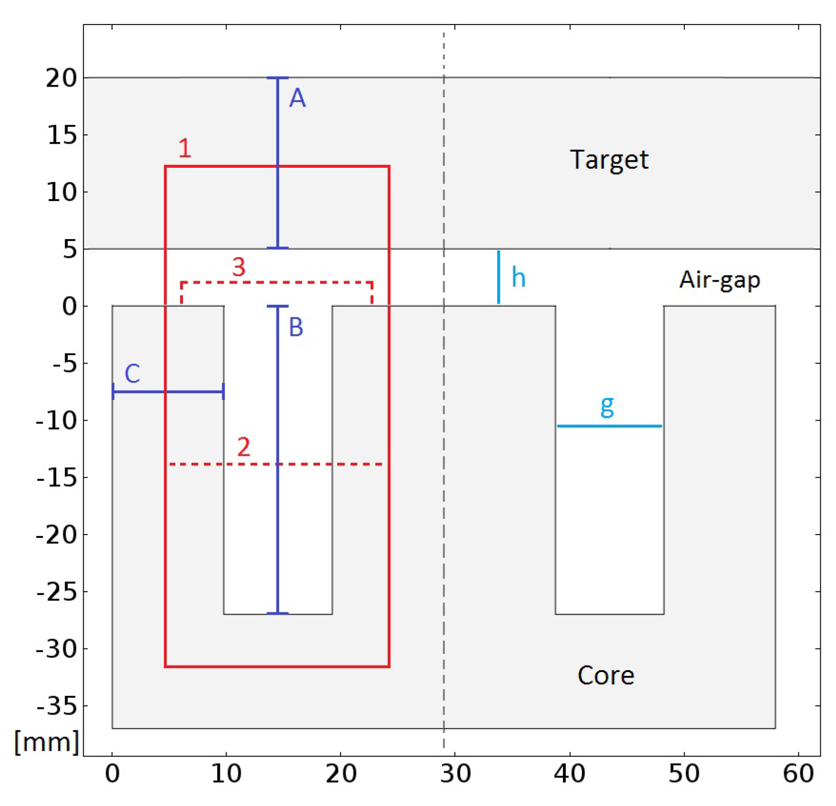
A good magnetic connection is here defined as a position of the electromagnet against the target that results in an initially high dynamic inductance, implying that the system reluctance is low (see Equation (4)), corresponding to a small h in Figure 7. Here, “initial” refers to a situation with zero or very low average current in the electromagnet, far from the saturation current. If the average DC current is then increased and the reluctance in the magnetic circuit is low enough, the electromagnet and target will begin to saturate. This increase in saturation will increase the system’s reluctance and can therefore be detected as a decrease of the dynamic inductance, if compared to the initial value.

Using the statements above, the following four-step procedure was adopted to detect not only if a good magnetic contact is present, but also if it is maintained:

• Step I:
  Obtain and save the open circuit dynamic inductance for the whole current range. This is done by simply making sure the tool is far away from any ferromagnetic object and then increasing the current step-wise, while taking measurements. In this experiment, this was done in 250 $\mathrm{m}\mathrm{A}$ steps. This only has to be done once, as the obtained values will not change, unless something drastically happens to the electromagnets.
• Step II:
  Continuously measure the dynamic inductance while moving the tool closer to the target, and if the inductance suddenly increases, a target has been found. Obtain and save the closed circuit dynamic inductance for the zero or low current, non-saturated case. In this setup, a lower limit of what was considered to be a “found target” was defined as a three-times increase of the inductance, compared to the open circuit inductance.
• Step III:
  Increase the current step-wise and take a measurement of the dynamic inductance at every current level. If a reduction larger than 25% of the maximal measured inductance is measured at any current step, mark the current level as the saturation point. If saturation is detected before the current reaches its maximum, the system will signal a success. Else, the system will flag a failure and issue a warning.
• Step IV:
  If Step III is successful, the robot is clear to begin moving. However, continue to measure the inductance and if the inductance unexpectedly drops to within 10% of the open loop inductance, the target has most likely been dropped, and a warning will be flagged.

3. Results

3.1. CCB Measurement Performance

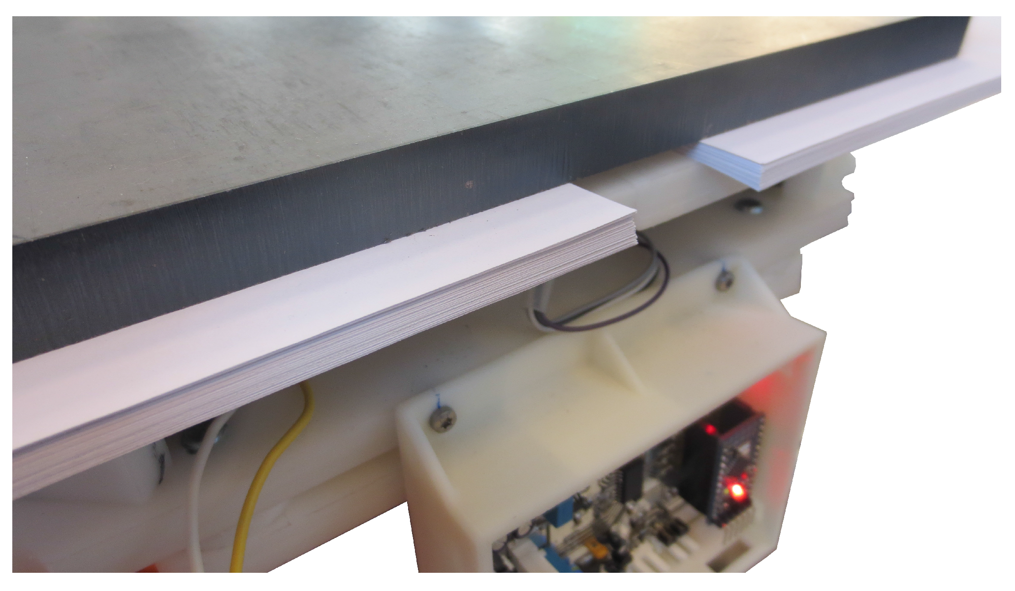
Evaluation of the CCB measurements was performed at 75 different air-gaps. In order to precisely control the length of each air-gap, sheets of standard A4 plain paper, each around 960 μm thick, were put between the electromagnets and target one at a time; see Figure 8. This was done as the specified robot accuracy of ±0.1 mm was deemed inadequate for calibration purposes. A measurement current ripple amplitude of 100 $\mathrm{m}\mathrm{A}$ was found to be large enough to give a good signal, yet low enough so that the target would not be lifted.

Measurements were performed in the air-gap range of 0–7.2 $\mathrm{m}\mathrm{m}$. Each measurement series was performed as a system start-up step response containing the first 2000 measurement points sampled at 300 $\mathrm{Hz}$. The raw rise-time measurements were then filtered using the filter implemented on the MCU. Both the filtered and unfiltered data were then sent to a host computer running a MATLAB script to record the data.

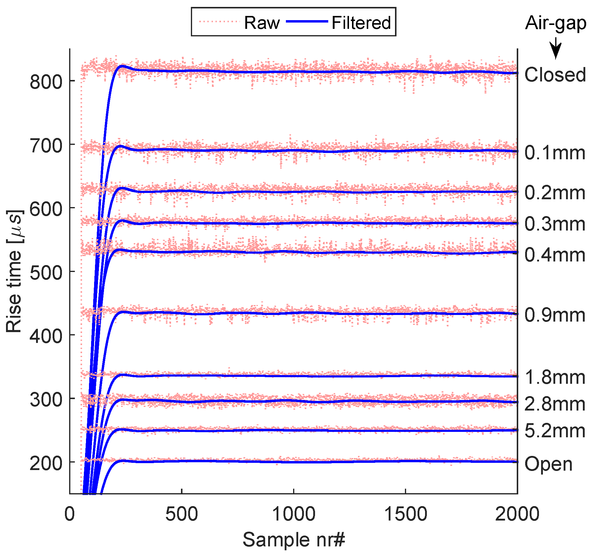
For calibration purposes, the filter cut-off frequency was set as low as possible, without causing numerical instability, and this frequency was found to be 5 $\mathrm{Hz}$. In normal operation, the filter was instead set to cut-off at 25 $\mathrm{Hz}$, giving a faster system response at the cost of lower accuracy. Figure 9 shows a comparison between the raw and filtered system start-up response.

The highest rise-time, around 820 μs, was measured with 0 $\mathrm{m}\mathrm{m}$ between the target and electromagnet. The second-to-last level, around 250 μs, was measured with an 5.2 $\mathrm{m}\mathrm{m}$ air-gap. Of the original 75 air-gap measurements, so was the difference (for the used excitation pulse of 100 $\mathrm{m}\mathrm{A}$) between each level, going from 5.2 $\mathrm{m}\mathrm{m}$–7.2 $\mathrm{m}\mathrm{m}$ (21 measurements in total), too small to be reliably separated from each other. To do so would require either a larger air-gap step, than 960 μm, or a less noisy measurement system. The final level, around 200 μs, was measured without a target at all, comparable to an infinite air-gap.

For the current measurements, no filtering was performed. The reason for this, as can be seen in Figure 10, was that the noise was only around 2.4 $\mathrm{m}\mathrm{A}$, translating to one LSB in the 12-bit ADC. The amplitude and difference of the two currents was also consistent for all tested air-gaps.

3.2. Rise-Time to Inductance

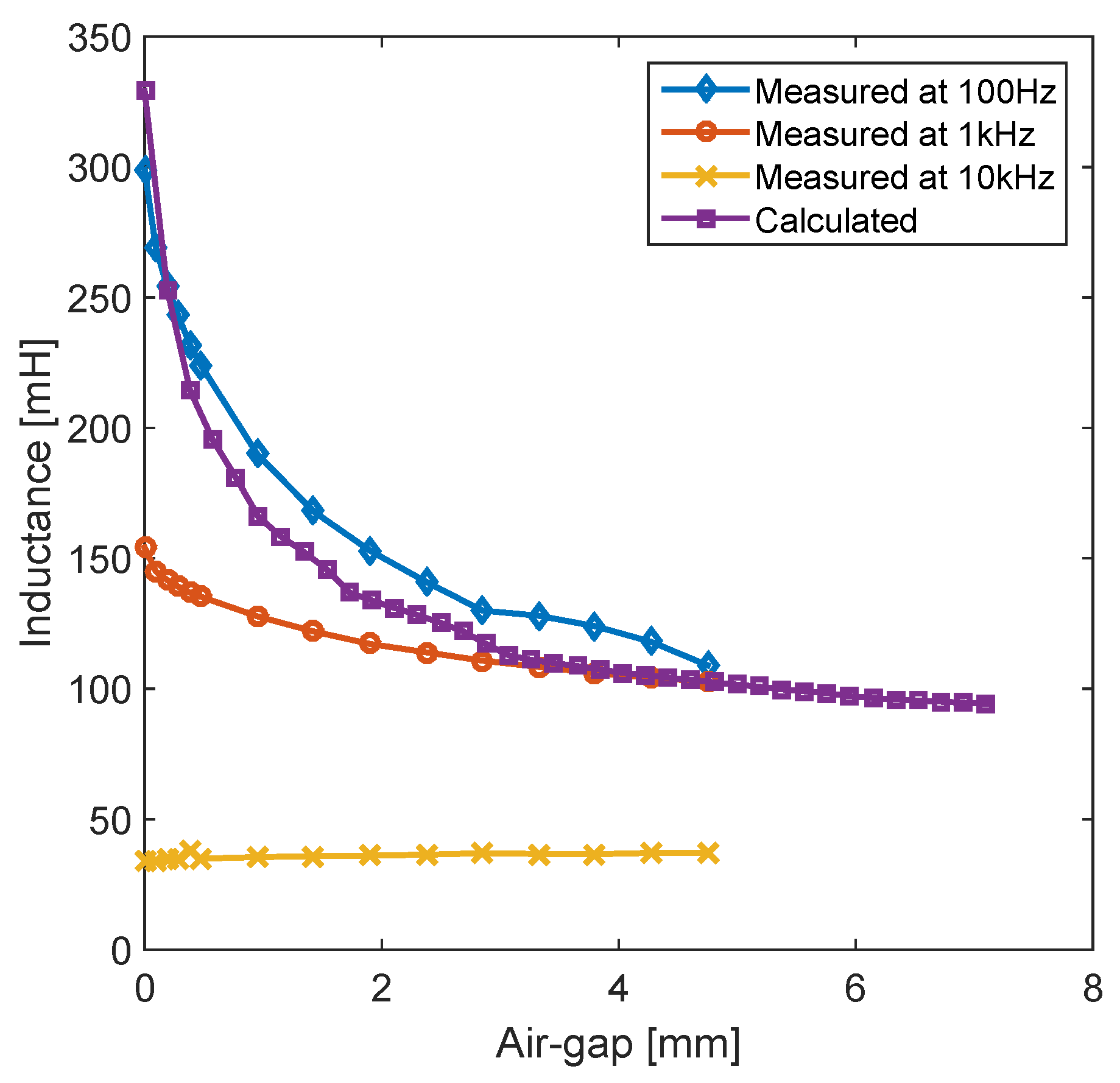
Shown in Figure 11 is a comparison between the calculated inductance, using Equation (3a) and the filtered CCB measurements, compared to the measured inductance using an inductance meter, Agilent-U1732A, using a 100 Hz, 1 kHz and 10 kHz excitation frequency. The calculated inductance using the hybrid Case 3 method shows best correspondence with the 100 Hz measurements, although the match is not perfect. Also note that the inductance is approximately constant for the 1 kHz and 10 kHz compared to the 100 Hz case; this is the main reason that a lower frequency measurement method was chosen. The materials present in this setup do not cope well with higher frequencies. The filtered data presented in Figure 9 have a standard mean deviation, σ, of 1.2 μs if the first 500 samples from each measurement series are ignored.

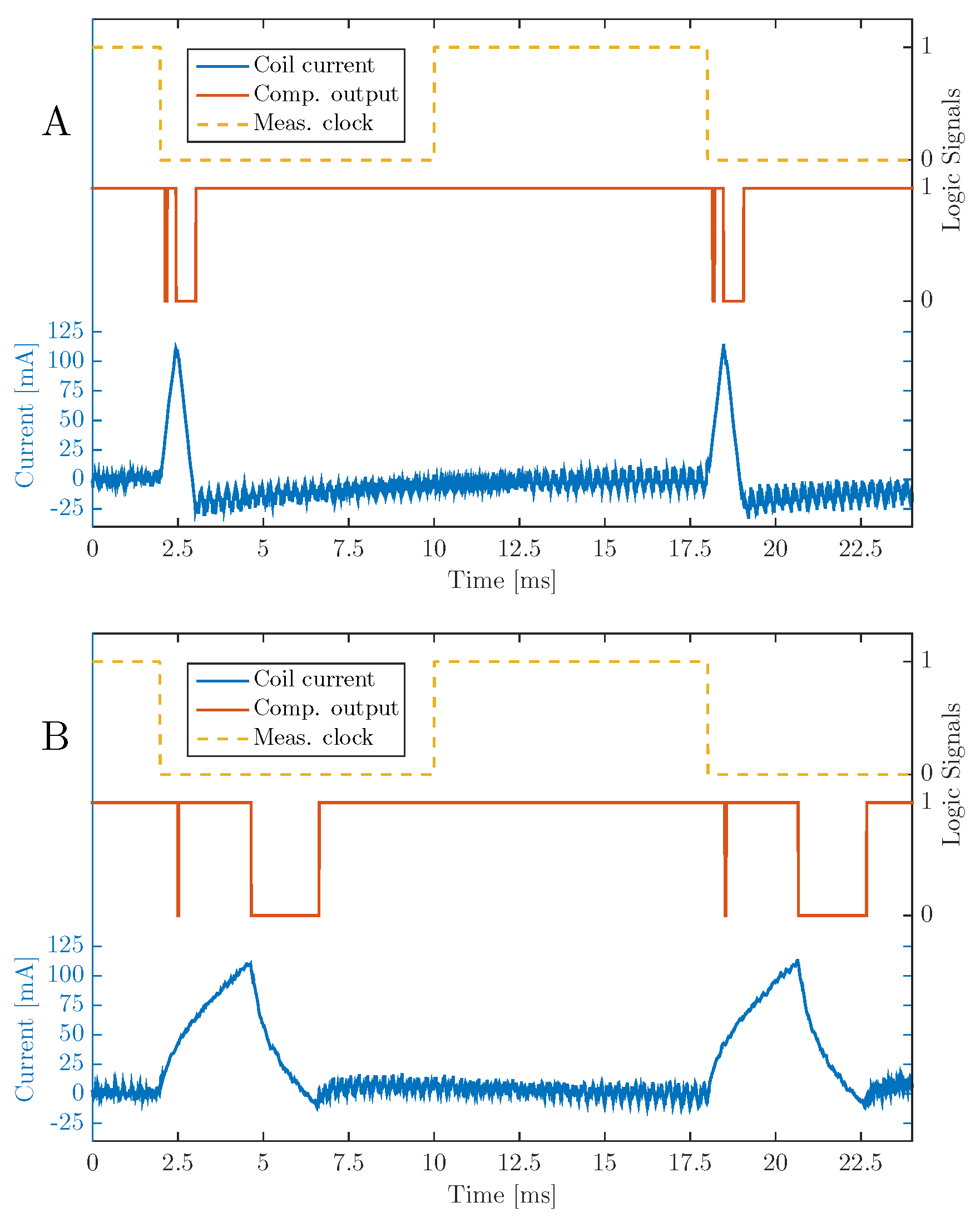
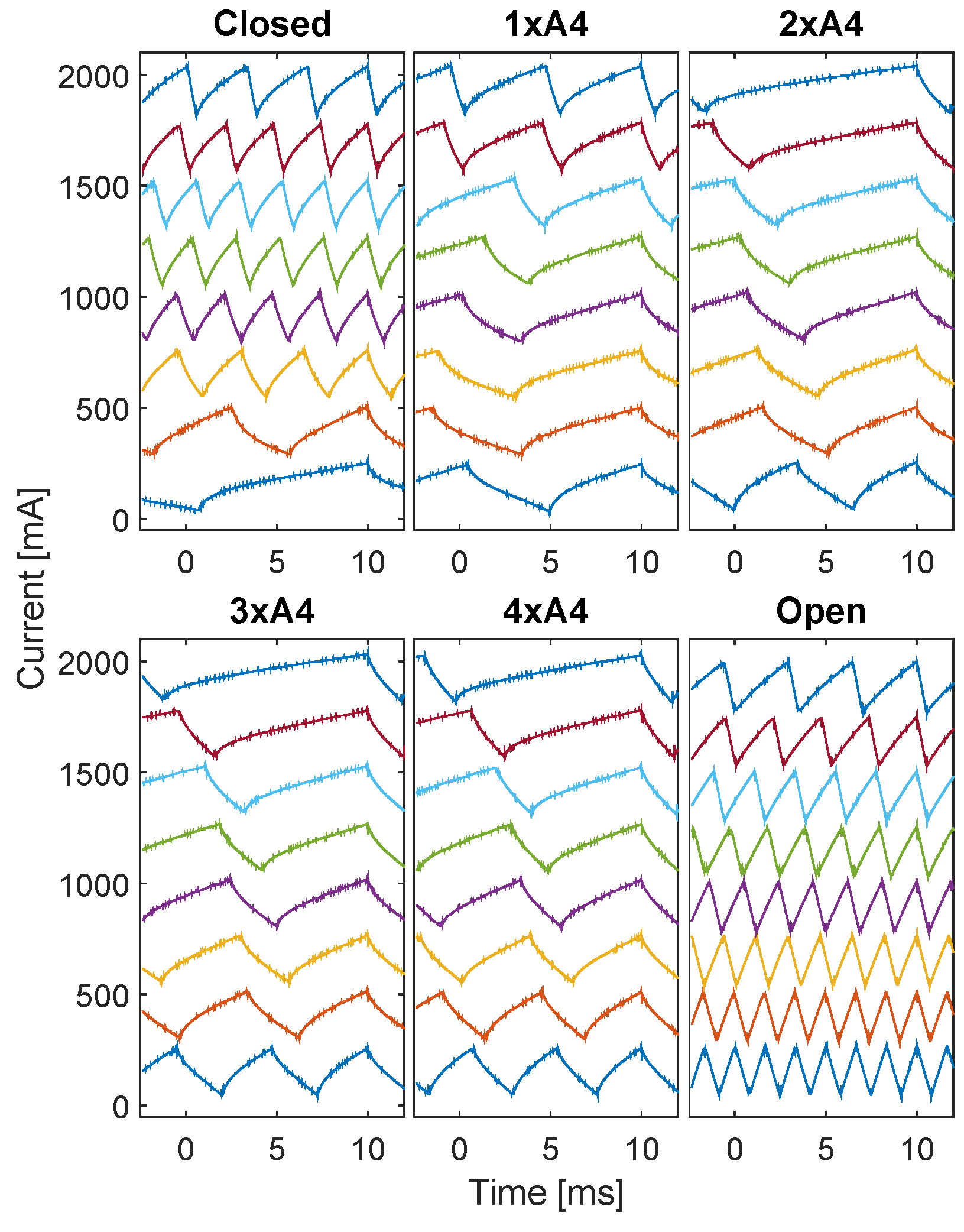
Next to get an estimate of the amplitude of the non-linear effects in the electromagnets and target, a series of measurements were performed at six different air-gaps and eight different currents; see Figure 12. To produce these waveforms, the control system was programmed to produce a constant 225 $\mathrm{m}\mathrm{A}$ current ripple, measured peak to peak, as opposed to the normal case where a big pulse would only be procured once every measurement period; see Figure 13. For each measurement, the current waveform was recorded using a Agilent-1146A current probe connected to a digital oscilloscope. It can be noted that the smaller the air-gap, the more distorted the waveforms becomes, in comparison to the decaying triangular current ripple predicted by an ideal RL-circuit. For the open-circuit case and low currents, the waveform shows almost ideal triangular behavior. For small air-gaps, most notable in the closed and 1×A4 case, the current rapidly rises after each switching. However, then, this effect dies out after around 1 $\mathrm{m}\mathrm{s}$, and the current derivative stabilizes to a more constant value, an effect assumed to be the result of decaying eddy currents. Most of these behaviors are attributed to the fact that the system contains a mixture of laminated and non-laminated iron in the same magnetic circuit, something that is not often covered in the basic theory.

For the closed case, increasing current also leads to an increased current-ripple frequency. This is partly due to saturation, as the inductance drops when the material begins to saturate, leading to an increased switching frequency in the hysteresis current control. However, a similar, but smaller effect can be seen in the open case. Here, the frequency difference is not due to saturation, but instead due to the increased resistive voltage drop in the coil, following the increase in current, effectively reducing the driving voltage. All cases are in reality a combination of the saturation and voltage drop effect, but an open or fully-saturated core will be dominated by the voltage drop effect.

3.3. Evaluation of Magnetic Contact

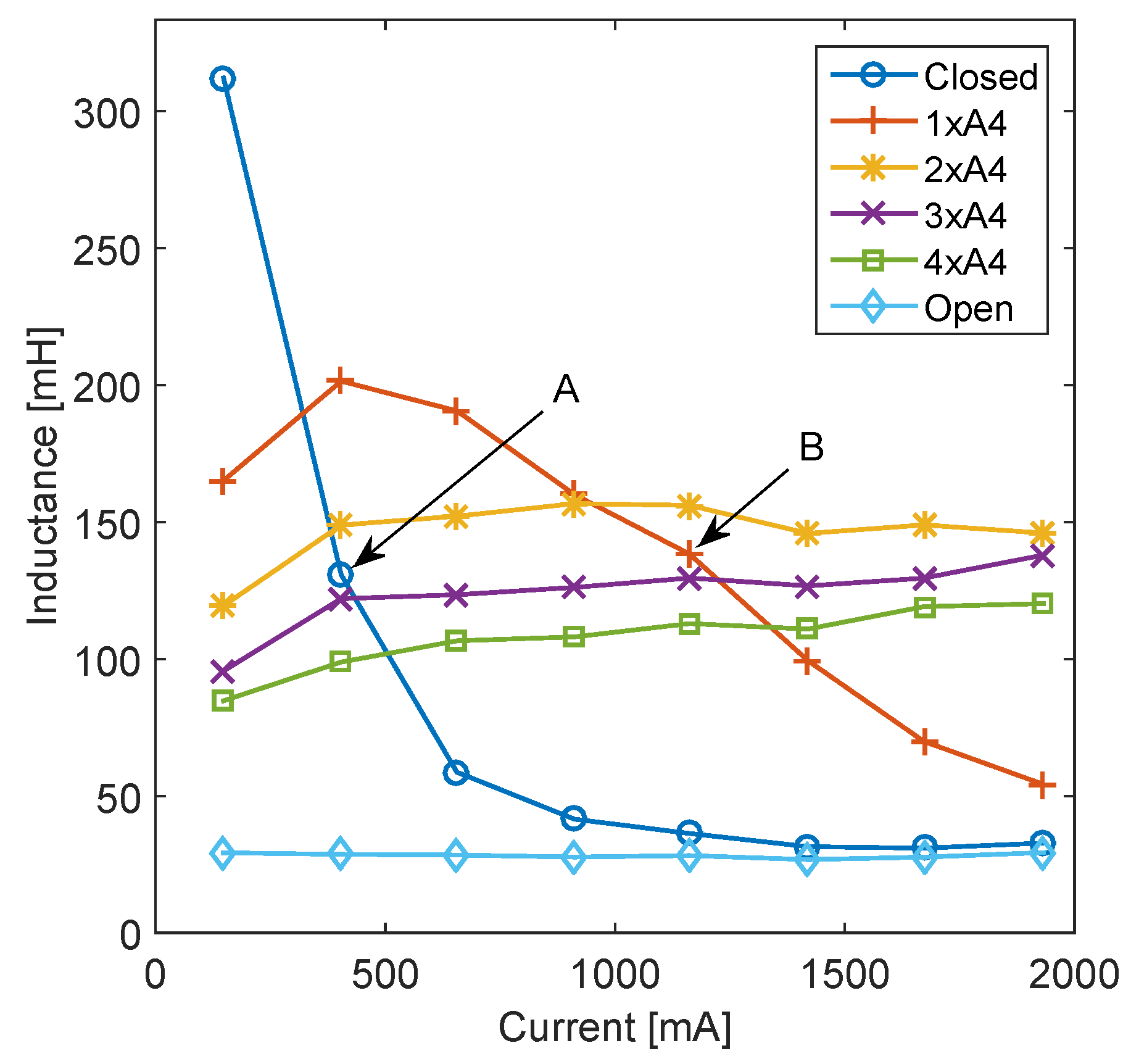
To verify the four-step saturation detection procedure, numerous measurements and calculations of the inductance were made at different currents and air-gaps. The results from this measurement series are shown in Figure 14. In the figure, it can be seen that in the open circuit, case the inductance starts at a relatively low value, 26 $\mathrm{m}\mathrm{H}$, and does not change much with increasing current. For the closed and 1×A4, case the inductance starts high, but then drops by approximately 280 $\mathrm{m}\mathrm{H}$ and 135 $\mathrm{m}\mathrm{H}$, respectively, at maximal current. The remaining intermediate air-gaps begin at medium values and show comparatively small changes, around 25 $\mathrm{m}\mathrm{H}$, over the whole current range. The marked points, A and B, are the points for the closed and 1×A4 case at which the saturation detection triggered (as the inductance shows a 25% decrease or more), making them the only two cases in this test that the robot would accept as successful.

Table 4. Normalized inductance for different air-gaps.

Magnetic Connection	Current (A)
	0.15	1.16	1.93
Good (closed)	10.9	1.3	1.1
Avg. (2×A4)	4.1	5.1	4.7
Bad (open)	1.0	1.1	1.3
	Norm. inductance

shows the normalized relation between the inductance, current and magnetic connection (air-gap). All inductances are normalized against the open loop inductance for the lowest current. This table indicates that a good magnetic connection, in this setup, can be characterized by an initially high normalized inductance that then rapidly drops as the current is increased. This is a behavior that easily can be detected using a microcontroller and few simple calculations.

The fact that the four A4 cases show an initial increase in inductance with increasing current might seem a bit strange. However, this has its explanation in that the increased current in turn generates an increased air-gap force. This force then, ever so slightly, compresses the paper and squeeze out any air that was left in the gap, leading to a smaller air-gap and, hence, larger inductance.

4. Discussion

4.1. CCB Measurements Performance

The implemented method of measuring the rise-time using a comparator and an DAC connected to a MCU showed that it is possible to measure the rise-time in an inductor using inexpensive and easily available components. The problem with measurement noise in the rise-time measurement was effectively handled by using a hybrid switching mode and a digital filter. The MCU was also able to send already filtered measurements to the master PC. Having the filter implemented directly in the MCU also opens the possibility to use the filtered measurement directly, for example to quickly react and change the current if the filtered value goes above a predefined threshold.

If this system is to be deployed in an industrial environment, it would be beneficial to also include a calibration procedure; this as the presented setup never proposed a way to extract the actual air-gap in mm from the inductance measurement. However, a rudimentary solution would be to implement a lookup table based on the calculated curve presented in Figure 11, but this approach would require manual calibration.

4.2. Rise-Time to Inductance

The curves presented in Figure 11 show that Equation (3a) can be used to find the inductance of a system, although one has to keep in mind that the solution is normally highly frequency dependent. The showcased measurement method, utilizing a hybrid switching mode, is comparable to that of measuring the inductance using a constant 100 $\mathrm{Hz}$ excitation frequency. Note, however, that this implementation will be mostly insensitive to what sampling frequency is used, as the large current ripple wave shape remains the same as long as the system have has sufficient time to stabilize after each large ripple. What is of more importance is that the ripple keep a constant amplitude, but as can be seen from Figure 10, the ripple amplitude is more or less constant using the comparator-based control system.

Eddy-currents are assumed to be the main culprit behind the distortions of the currents shown in Figure 12. This will have negative effects on the accuracy of Equation (3a), as the implemented inductance model does not account for this behavior. This implies that the calculated inductance values for small air-gaps will be less accurate than those calculated for big air-gaps. Exactly how big of a difference this makes remains an open question.

4.3. Magnetic Contact

While the presented approach does not give an absolute value for the lifting force, it does give a useful estimate of the magnetic contact between the electromagnet and target, something that a normal inductive sensor cannot do. Once calibrated, minimal computational power is required to evaluate the current state of the system. A lookup table similar to that of Table 4 alongside a few stored measurement values would be enough to determine if a good or bad connection has been obtained or lost, a setup easily implemented in a low power MCU. Interesting to note is that if the core is fully saturated, as in the closed case for currents above 1.2 $\mathrm{A}$ in Figure 14, a dropped target is indistinguishable from an open circuit. Therefore, the current has to be kept under the level of full saturation in order for this function to work. Keeping the current under the saturation point will reduce the contact force, but in this specific setup, this is not a problem as the used electromagnets are over-dimensioned. Each electromagnet is specified to lift 650 $\mathrm{k}\mathrm{g}$ at rated current, where the task only requires 120 $\mathrm{k}\mathrm{g}$ in total. However, in the general case, this is something that must be considered.

5. Future Work

Two main areas are suggested for further investigation and development.

The first is that the CCB could benefit from an upgrade of the MCU. New low cost alternatives are available that have much more computational power, such as the MK20DX256, a 32-bit ARM-based MCU, as compared to the current eight-bit MCU. An upgrade from 12-bit ADC and DACs to 16-bit versions would also allow for a higher resolution in the current measurement and, hence, also, the following inductance calculations. Further savings could also be done in the H bridge implementation, where more highly integrated circuits, such as the MC33887 or BTN8982TA could be used to reduce the amount of individual components.

The second area is to improve the inductance model, so that it includes the non-linear effects of switching showcased in Figure 12. The focus should be on modeling the influence of eddy-currents on the inductance, how to deal with mixed magnetic materials and, if possible, also include the effects of saturation. This without having to go into numerical methods and FEM as computational power remains limited. Expanding the model to directly convert the rise-time and current measurements to the mm air-gap would also be a useful feature.

6. Conclusions

A self-sensing electromagnetic robotic tool has been constructed, and its performance has been evaluated. The sensing functionality uses low cost electronics and a hybrid switching mode to produce temporary current ripples in order to increase accuracy. Derived equations and models have been tested and verified against real-world measurements. Using a standard electromagnet, as a distance sensor, against an unlaminated target has been shown to work in the range of 0 mm to 5.2 mm. A method to determine if the electromagnet has a good or bad magnetic connection to the target requiring minimal computational effort was also presented. This low cost sensor implementation will be a useful tool in the future automation technology development aimed at enabling the mass production of linear wave-power generators.