
Detector Characterization and Mitigation of Noise in Ground-Based Gravitational-Wave Interferometers


1
LIGO, California Institute of Technology, Pasadena, CA 91125, USA
2
Department of Physics, Computer Science, and Engineering, Christopher Newport University, Newport News, VA 23606, USA
*
Author to whom correspondence should be addressed.
Galaxies 2022, 10(1), 12; https://doi.org/10.3390/galaxies10010012
Submission received: 17 December 2021
/
Revised: 7 January 2022
/
Accepted: 10 January 2022
/
Published: 14 January 2022
(This article belongs to the Special Issue Present and Future of Gravitational Wave Astronomy)
Abstract
:Since the early stages of operation of ground-based gravitational-wave interferometers, careful monitoring of these detectors has been an important component of their successful operation and observations. Characterization of gravitational-wave detectors blends computational and instrumental methods of investigating the detector performance. These efforts focus both on identifying ways to improve detector sensitivity for future observations and understand the non-idealized features in data that has already been recorded. Alongside a focus on the detectors themselves, detector characterization includes careful studies of how astrophysical analyses are affected by different data quality issues. This article presents an overview of the multifaceted aspects of the characterization of interferometric gravitational-wave detectors, including investigations of instrumental performance, characterization of interferometer data quality, and the identification and mitigation of data quality issues that impact analysis of gravitational-wave events. Looking forward, we discuss efforts to adapt current detector characterization methods to meet the changing needs of gravitational-wave astronomy.
Keywords:
LIGO; Virgo; KAGRA; gravitational waves; detector characterization; data quality; noise mitigation1. Introduction
Within the past decade, advances in the design of gravitational-wave interferometers have allowed the Advanced LIGO and Advanced Virgo detectors to reach the required sensitivity to detect gravitational waves from astrophysical sources [1,2]. These observations [3,4,5,6,7] of the cataclysmic mergers of massive compact objects allowed for the discovery of a new population of black holes [8], insights into the nuclear equation of state [9], precision tests of general relativity [10], and the identification of compact objects that are not predicted to form from stellar evolution [11,12].
These historic discoveries in astrophysics have required measurements of gravitational-wave strains of less than [3]. To achieve these levels of sensitivity, gravitational-wave detectors rely on a wide array of technologies designed to minimize the sensitivity of the detectors to non-astrophysical sources of noise. However, the complexity of the detectors also provides numerous pathways for introducing instrumental noise into the recorded data. Addressing the presence of noise in the instruments is a crucial aspect of gravitational-wave astrophysics, both for the continual improvement of the detectors themselves and for ensuring appropriate treatment of the noise in the data analyses.
This area of research, focusing on diagnosing and mitigating instrumental problems that impact the quality of recorded gravitational-wave strain data, is known as “detector characterization”. Detector characterization was a central element of the initial operation of both first [13,14,15] and second [16] generation detectors and the first detection of gravitational waves [17]. Figure 1 illustrates the central role of characterizing the detector and its data quality to the flow of LIGO data analysis from the instruments to the final output of gravitational-wave catalogs. As gravitational-wave astronomy grows, detector characterization and noise mitigation continue to play an important role in the maximization of detector sensitivity and analysis precision [15,18,19].
This article reviews the current state of detector characterization and noise mitigation used in gravitational-wave science. Section 2 focuses on the techniques and approaches to characterizing instrumental performance of gravitational-wave interferometers. Section 3 discusses how problems with the data quality are diagnosed and how this information is propagated to gravitational-wave data analyses. Section 4 focuses on the detector characterization steps taken in response to detected gravitational-wave events. Section 5 then provides an overview of current techniques used to mitigate the impact of instrumental noise in the data. Finally, Section 6 remarks on the current state of the field and potential applicability of these methods to future detectors and analyses.
The focus of this work primarily focuses on techniques used in analyses of data from the LIGO Hanford and LIGO Livingston detectors and analyses completed by the LIGO-Virgo-KAGRA (LVK) collaborations, with examples related to the Virgo detector included when relevant. However, the methods described are broadly applicable to other current and future ground-based interferometric detectors, including GEO600 [20], KAGRA [21], and LIGO India [22] and analyses completed by other groups. All gravitational-wave strain data used for visualizations in this work is from the Gravitational-wave Open Science Center (GWOSC) [23].
Figure 1.
A visualization of the connections between different components of gravitational-wave data analysis. Detector characterization is in the middle, indicating its critical role in gravitational-wave astronomy, as it contributes to many different steps of the process, from improving the detectors to checking candidate gravitational-wave signals for any possible pollution by nose artifacts. Figure reproduced from [24]. © IOP Publishing. Reproduced with permission. All rights reserved.

2. Characterizing Gravitational-Wave Detector Instrumentation
One central goal of detector characterization is finding sources of noise within the instruments and working with on-site staff to mitigate these noise sources to improve the detectors’ performance. These investigations may be targeted on improving specific subsystems of the detector or diagnosing particular kinds of noise. This section presents an overview of instrumental investigations for the purposes of making concrete improvements to the detectors, including the detailed analysis of individual detector components and methods for investigating transient and persistent noise in the detectors.
2.1. Subsystem Characterization
Characterization of the instruments for the purpose of improving instrumental performance is carried out at various levels of specificity. To be able to truly characterize the detector as a whole, first individual components have to be well understood, and then the connections between individual subsystems and how they connect to the final output of the detector. Components of each detector are classified into multiple “subsystems” that each focus on a specific element of the overall detector design. The instrumentalists, commissioners, and engineers working on site are faced with the monumental endeavor of finely tuning each subsystem and getting the many different components of the detector to work together in the precise harmony needed to detect gravitational waves. Detector characterization of the individual components of the detector is an integral part of the process, even before the full detector has been installed. Analyzing the data of specific subsystems or combinations of subsystems prior to observing runs is necessary for diagnosing problems and improving the instruments.
For each subsystem, it is important to know its key design features, the important data channels used to monitor its performance, and to develop methods of distinguishing abnormal and nominal behavior. Detailed studies of each subsystem have continued from the earliest engineering runs that were used to characterize the detector and continue to be an important part of the process of identifying issues in the detector during observation runs to detect gravitational waves. This includes having a deep understanding of the physical environment surrounding each instrument [25], the seismic isolation system [26], the suspension systems [27,28], the pre-stabilized laser, individual optical cavities, calibration, thermal compensation system, and the many feedback and control loops required to operate the detectors. At such a detailed level of characterizing the detector, there can be impacts not only on diagnosing specific issues at an early stage of commissioning the detectors, but also on the design of future detectors. For example, the highly sophisticated seismic isolation systems of Advanced LIGO were motivated by an understanding of the significant impact of seismic noise in initial LIGO [29].
2.2. Diagnosing and Mitigating Transient Noise
Characterization of transient noise in the detectors takes into account the overall detector output as well as the behavior of individual subsystems. Several existing papers describe examples of noise investigations in detail [16,18,30,31,32]. Given the complexity of the detectors and the wide variety of potential noise sources, there is no single way to diagnose all types of instrumental noise. However, these studies tend to follow a similar process, which we describe here. A general overview of this process is shown in Figure 2. These investigations can be focused on tests completed at the detector site or remotely using recorded data and include identification, characterization, and mitigation of instrumental problems. There is generally active collaboration between those at the sites investigating the detectors and those analyzing the detector data, such as diagnostic tests completed by those on site being evaluated by people off-site with additional data analysis tools.
The initial identification of a problem typically begins with analysis of the output of the detector and gathering basic observations about the patterns in the noise, which often gives some initial clues when combined with knowledge of the detector and its environment. This initial analysis is frequently done with the aid of one or more of the many software tools that are run automatically on a daily basis, whose results are displayed on summary web pages internal to LIGO and Virgo and inspected regularly [33,34]. Several of the summary pages show key figures of merit that describe the overall sensitivity and data quality of the strain channel, while numerous additional pages include detailed figures that can be used to trace noise through various subsystems.
One indication of a new problem in the detector is an increase in the rate of “glitches” (short-duration bursts of noise) in the strain data at a particular time or frequency. “Event trigger generators” search for glitches in a time series. One of the most commonly used event trigger generators for detector characterization is Omicron, which is run automatically on a daily basis for the strain channel as well as thousands of auxiliary channels [35,36]. Omicron uses a wavelet basis to transform the time series into a time-frequency representation. Omicron records a variety of metrics for each glitch that it finds, including the peak time, frequency, and signal-to-noise ratio (SNR). Additional event trigger generators are DMT Omega and KleineWelle [37]. Problematic populations of glitches may also be identified by characterizing outliers in the gravitational-wave search backgrounds [17,38] or single-detector GW searches [39,40].
Identified patterns of the noise, such as glitches occurring in a particular frequency range or only during certain times of the day, can already provide useful information about the noise. Combining this knowledge with prior knowledge of the detector based on subsystem characterization or previous instrumental investigations can offer some clues as to the source of the noise. For example, low frequency glitches occurring particularly during the weekdays could relate to elevated seismic noise from human activity.
In addition to the characteristic frequency and SNR of glitches, it is also useful to know the frequency morphology over time. The “Qscan” method [41,42] is based on a similar algorithm to Omicron, and uses overlapping time-frequency tiles of varying widths to create a high resolution spectrogram that shows how the glitch’s frequency and amplitude evolve over a short time scale. Based on these images, different classes of glitches have quite distinct shapes, as illustrated in Figure 3.
Since the early science runs of LIGO and Virgo, the detector characterization group began to develop an understanding of particular glitch classes [14,43,44]. Throughout the observing runs, detailed investigations of specific types of glitches (such as “whistle” glitches [16], “blips” [45], and “scattered light glitches” [46]) have continued to be an important facet of detector characterization. These investigations frequently begin with noticing the impact on data quality in the searches, rather than at the specific level of detail of characterizing a particular instrumental monitor. In the noise investigation process, these glitches might be classified visually, but there are now also glitch classification tools that were developed to aid in creating categories of glitches. Gravity Spy [47,48,49] is a citizen science and machine learning project that offers categorization of glitches based on their appearance in the Qscans. The Gravity Spy glitch collections have been helpful in noise investigations, for example in a study of scattered light glitches that led to improvements in the detector in the third observing run [46].
To gather more data on the specific parts of the detectors contributing to transient noise, results of automated correlation or classification algorithms can reveal more information, along with knowledge about the detectors to interpret results. Statistical methods are used to compare glitches in the gravitational-wave strain channel with glitches in auxiliary channels [50,51,52,53]. There are also methods specifically targeted to identify the source of specific types of noise, such as scattered light [54,55] or lightning [56,57,58,59].
Among the algorithms for making statistical comparisons between channels, the Hierarchical Veto (HVeto [25,60,61,62]) method is especially used for instrumental noise investigations in LIGO. This algorithm begins with the set of all the Omicron triggers in the main gravitational-wave channel and then finds statistically significant time coincidences with glitches in other channels. The hierarchical nature of the method means that it performs multiple rounds of analysis, and after each round it removes the glitches that were found to be correlated with the most significant auxiliary channel. Successive rounds will typically pick up on different types of glitches. The results further include lists of channels that are all related to the most significant channels, and Qscans of the glitches in each round.
Careful studies of the environment around each detector can also further inform the potential sources of transient noise. During each observing run, a series of “injections” that simulate excess environmental noise are regularly performed at each site [25,60,61,62]. These injections include inducing magnetic noise, loud sounds, and excessive shaking at a level of excitation significantly exceeding the normal environmental level but within the dynamic range of the detector. These injection studies are only completed during time periods when the detector is not actively observing, as they add large amounts of additional noise to the detector data. The coupling between each noise source and the detector can be calculated by measuring the amplitude of the injection using monitors of the physical environment and comparing this to the amount of noise seen in the gravitational-wave strain channel. These measurements allow scientists to know if any sources of noise in the local environment are strong enough to impact the gravitational-wave strain data. If the transfer function between a particular noise source and the detector strain is linear, then the measured coupling is sufficient to estimate the amount of noise each source adds to the detector data. While some noise sources, such as scattered light, do not have a linear coupling, the majority of sources from the local environment are indeed linearly related to the detector strain.
These various methods are used in concert to perform investigations of particular types of glitches, with each method providing particular clues that eventually lead to a deeper understanding of the channels involved in the noise. However, none of the algorithms on their own can provide a solution to the problem without additional knowledge of how the channels are related to the complex inner workings of the detectors, a working knowledge of how noise propagates through the various instrumental systems, and additional targeted analyses of the noise. For example, Figure 4 shows a follow-up study that was done to diagnose a population of glitches in the strain channel that was traced to a compressor switching on and off. This knowledge is built up over time through investigations on the subsystem level, noise injections, and communication with instrumental experts.
Finally, targeted investigations on site at the detector are generally applied to further confirm the specific cause of a noise source. These investigations could be types of noise injections to try to simulate the glitch. For example, in the famous thirsty ravens investigations [31], scientists simulated the effects of ravens pecking, and then observed how this introduced similar glitches in the detector.
2.3. Diagnosing and Mitigating Persistent Noise
In addition to investigating glitches in the detector, instrumental investigations also target long-term persistent noise in the detector. Improving the overall sensitivity allows us to see farther into the universe in all types of gravitational wave searches. Lowering the overall noise in the detectors, reducing extra noise at specific frequencies, and keeping the detectors running in a stable state are especially critical for searches for persistent gravitational-wave sources.
Characterization of persistent noise follows a similar process to transient noise investigations, with identification of problematic noise from summary plots of the main output of the detector, gathering information from automated algorithms searching for correlations with auxiliary channels, synthesis of the results from these algorithms with prior knowledge of the detectors, and targeted investigations to continue to build up that knowledge. The types of tools used for these steps of the investigations are different though.
Persistent noise at constant frequencies, or “lines”, can be particularly harmful for searches for continuous gravitational waves. Tracking lines in the data and keeping lists of known sources of lines is an important part of the instrumental investigation process [64]. The FScan [65], NoEMi [66], and FineTooth [64] tools are used to track lines in the strain channel and auxiliary channels. FScan produces spectra and spectrograms for each day, and NoEMi tracks lines, follows wandering lines (which change in frequency over time), and indicates coincidences with occurrences in auxiliary channels. Often groups of lines are found to have a constant frequency separation between adjacent lines and are referred to as “combs”. FineTooth is a tool for finding and tracking combs of lines in the strain channel as well as magnetometers, which have proven to be useful witnesses of electronics noise that manifests itself in combs. Additionally, noise investigations of lines and combs are frequently aided by analyzing the correlation between the strain channel and auxiliary monitors at specific frequencies, to narrow down the potential sources of noise. In cases when the time in the observing run that the line first appeared can be identified, it is also possible to use the list of instrumental upgrades that occurred near that period to narrow down the search.
Although the long-term performance of the detector is particularly relevant for detecting persistent sources of gravitational waves, numerous metrics were developed to characterize the long-term performance of the ability of each detector to observe transient gravitational-waves. One key figure of merit that describes the overall sensitivity of the detector is the binary neutron star (BNS) “range”, a measure of the distance to which the detector could detect a binary neutron star inspiral at an SNR of 8 at any given time, averaged over the entire sky and the different gravitational-wave polarizations. The BNS range fluctuates over time with the noise in the detectors, and significant drops in the BNS range over long periods of time can sometimes be a first clue that something is wrong in the detectors. Detector characterization experts study fluctuations in sensitivity [67] in order to provide clues about what noise sources could be affecting the range of the detector. These investigations are conducted in order to increase the stability of the detectors and maximize their sensitivity, in order to increase the effectiveness of all types of gravitational-wave searches.
The same environmental conditions that lead to changes in the detector range can also lead to a decrease in the amount of time that the detectors are actually in a state that is able to record observational-quality data. Severe environmental disturbances such as nearby earthquakes (or severe earthquakes even far away!) can make the detectors lose the carefully tuned and aligned resonances in the optical cavities required to operate the detector. This loss in observing time affects all astrophysical analyses, so an important aspect of detector characterization is analyzing how the detectors’ stability can be increased to be more resilient to such effects. Investigations of the detectors’ “duty cycle” are aimed at increasing the amount of time that the detectors are actually operational [68,69]. For example, when an earthquake is known to be coming (based on data from far away seismometers), the detectors can be placed temporarily in an “Earthquake mode”, a modified seismic control scheme which allows the detectors to maintain arm cavity resonance during more earthquakes, therefore increasing the amount of usable data [70].
Noise sources that may not be strong enough to be observed in a single detector can still be particularly troublesome if the noise is correlated between detectors. Typically, multiple detectors are used to identify gravitational-wave signals and it is assumed in many analyses that no correlations exist between data from different detectors. Hence, any strongly correlated noise sources that are not accounted for could bias current gravitational-wave analyses. Although multiple potential sources for correlated noise were suggested [17], the only source of noise known to be relevant for ground-based detectors is magnetic noise from “Schumann resonances” [71], fluctuations in the Earth’s magnetic field, and strong lighting strikes [72]. The noise contribution from these resonances is currently too low to impact searches for gravitational waves with current detectors, but will become more relevant in the future as detectors increase in sensitivity [73]. Regardless of their expected impact, the noise contributions from correlated magnetic noise is closely monitored using magnetometers and measurements of the coupling between magnetic noise and the strain data at each observatory [18,74].
3. Gravitational-Wave Data Quality
Data quality issues that have not been mitigated in the instrument can be vetoed from the data that is analyzed if these data quality issues can be confidently separated from astrophysical signals. Whether or not data are vetoed depends on several factors, such as the severity of the known problems with the data, the impact of the data quality issues on the astrophysical search backgrounds, and the ability to construct a veto that efficiently removes times of poor data quality without throwing away too much data. This section details how data quality issues are identified and how this information is propagated to gravitational-wave analyses.
3.1. Data Quality Impacts on Searches for Transient Gravitational-Waves
Transient sources of gravitational waves include signals from compact binaries coalescences (CBCs) [3] and other high-energy astrophysical phenomenon, such as supernovae [75]. Searches for these transient gravitational waves must separate bursts of excess power due to gravitational-wave signals from instrumental artifacts. A variety of pipelines were developed that have been used in analyses by both the LVK [76,77,78,79,80,81] and other groups [82,83]. These searches primarily incorporate information about the data quality using “data quality vetoes”, which identify time periods where the data have a high probability of corruption by glitches.
The process of developing data quality vetoes frequently begins much in the same way as general instrumental noise investigations: excess noise is identified through automated pipelines and then traced to try to find correlations with auxiliary monitors. However, in developing data quality vetoes, the primary emphasis is on improving search results rather than improving the detector, so rather than being concerned with any glitches or excess noise, the noise is viewed first from the lens of the search pipelines. For example, if search pipelines show an excessive number of outliers that are due to instrumental artifacts rather than astrophysical signals, there will be more motivation to develop a veto to eliminate the noise. After the initial identification of the problem, similar tools are used to provide a clear picture of when that type of problem occurs, for example using Omicron [35,36] to gather all the glitch times, and Hveto [50,51] or iDQ [53] to find correlations with auxiliary witnesses, often alongside the investigations into the source of different noise source that were discussed in Section 2.
Data quality vetoes are typically applied in separate categories at different points in the search pipeline, and are individualized based on the different types of searches. In recent observing runs, three categories of veto were used, referred to as “category 1”, “category 2”, and “category 3”. In all searches, the first category of veto, category 1, includes data that is deemed to be completely unusable and unreliable, which is eliminated before any of the search pipeline is conducted. Beyond this most severe category of data quality vetoes, other data quality cuts are tuned carefully based on how the noise impacts the different search pipelines. Category 2 vetoes are developed to target small time periods around specific types of glitches, while category 3 vetoes are based on statistical correlations between auxiliary channels and the gravitational-wave strain data. The process for creating data quality vetoes and their impact on the total spacetime volume that searches for compact binary coalescences are sensitive to (referred to as the “sensitivity” of a search) is described in greater detail in [38,84].
Several common strategies exist for creating data quality vetoes. One strategy, which is especially employed in the creation of category 1 vetoes, is to determine segments manually, based on known severe or unusual environmental or instrumental disturbances at a very specific time. The times of these vetoes are frequently taken from the online detector logbook. Examples of this kind of manual determination from O3 are times when forklifts, cranes, or large trucks were operating near the detectors during observing mode [85].
Many types of noise, however, are recurrent and require vetoes to be more finely tuned and programmed in order to select all of the data that needs to be cut. This is how category 2 vetoes are generally developed. Ideally, the noise is traced to a correlated auxiliary witness signal, which can be used to predict any time the noise appears in the strain data. For some types of vetoes, this will involve creating a threshold on an auxiliary witness time series. An example of this type of threshold is shown in Figure 5. For other types of glitches, vetoed times are determined by auxiliary Omicron triggers, usually after a correlation was found by Hveto or a similar algorithm. Whether these vetoes are built using Omicron triggers, an auxiliary channel, or some processing of an auxiliary channel, the exact veto parameters are tuned carefully to maximize the ratio of efficiency (the percent of glitches removed) to deadtime (the percent of total time removed). This ensures that the veto is capturing the most noise while minimizing the risk of removing astrophysical signals.
One important consideration in development of data quality vetoes is to make the primary determination based on auxiliary data and the astrophysical search backgrounds, without using the strain data itself. The exception to this is in cases where there is severely loud noise or noise present in the data which is much louder (e.g., by an order of magnitude) than could be reasonably expected of an astrophysical signal. For the CBC searches, loud glitches are removed from the data before analysis using “gating”, described in Section 5.
The channels used to produce vetoes must also be determined to be ‘safe” for vetoes, meaning that they are truly witnesses only of auxiliary information, and they will not be influenced by the strain data through control loop feedback. This is important to ensure that the witnesses will only veto noise, not astrophysical signals. The safety of channels is determined by injecting strain noise into the detectors by physically moving the test masses with a known frequency and amplitude [86]. Data from auxiliary channels is then searched for evidence that this injected noise propagated into other channels. If such evidence if found, these channels are not deemed safe.
Different search pipelines make additional data quality cuts or implement additional signal consistency checks or the results of other algorithms, based on the needs determined by reviewing each search’s background noise. Searches for generic transient gravitational-wave signals (“bursts”) for example, directly use the results of Hveto in their data quality cuts as a category 3 veto.
The amount of time vetoed from the analyses has varied slightly over the different observing runs of Advanced LIGO and different analyses, but typically the total time vetoed is on the order of ∼2% or less. In the first observing run, there were several periods of very poor data quality at the Hanford observatory traced to one particular noise source, which ultimately led to vetoing 4.6% of the coincident detector time as a category 1 veto [17]. However, other data quality vetoes and subsequent observing runs have removed less data. In the second and third observing runs, the vetoes have removed ∼1–2% of the data in total [5,7,18]. Of the confident events identified in the first three observing runs by LVK analyses [4,5,6,7], only 2 events have overlapped data quality veto segments. Considering the amount of time removed by these vetoes and the total number of detected events, this number is consistent with the expected rate of chance coincidences. Furthermore, multiple detectors in operation and the diversity of methods that data quality vetoes are used in analyses allowed these events to still be detected despite the overlap with a veto.
The benefits of data quality vetoes were reduced in recent observing runs due to improvements in how search pipelines address glitches in the data. In analyses of data from the first observing run, data quality vetoes increased the sensitivity of a search for CBC signals by up to ∼50% [38]. However, the sensitivity of the same search pipeline in the third observing run increased by only ∼5% [18]. As noted in the previous paragraph, the amount of time removed by data quality vetoes changed by only a few percent across these observing runs, suggesting that the difference in sensitivity increase is due to improvements to the search pipeline that were implemented between the two periods considered based on the understanding of detector data from the investigations discussed in this review. One such improvement is accounting for how glitches in the data are similar to only a small portion of the CBC parameter space [87,88]. This change meant that the presence of glitches only reduced the sensitivity of the search in a small portion of the parameter space, which in turn reduced the benefits of mitigating glitches with data quality vetoes. For this reason, it is expected that data quality vetoes will be needed less frequently in future CBC searches. Searches for gravitational-wave bursts have also made improvements that have reduced the benefits of data quality vetoes, but to a lesser extent. Data quality vetoes still significantly improve the sensitivity of burst searches as burst waveforms are more general than CBC waveforms and hence are more likely to be similar to detector artifacts.
In addition to data quality vetoes, another data quality product, the iDQ timeseries, was used in analyses of LIGO data in the third observing run. The iDQ algorithm analyzes the detector state using auxiliary channel information using machine learning techniques to determine the likelihood that there is a glitch present in the strain data. These predictions are made for all times and stored as a time series with a sample rate of 128 Hz. Figure 6 shows an example of the iDQ timeseries near a glitch and near a gravitational-wave signal. At the time of the glitch, the likelihood of a glitch (as predicted by iDQ) is elevated. As expected, no such increase in likelihood is seen at the time of a gravitational-wave signal.
As of the end of the third observing run, only one search algorithm, GstLAL [77], has incorporated this iDQ time series. This CBC search used the value of the iDQ time series to down rank candidates that were predicted to be likely glitches [89]. This method contrasts the approach used with data quality vetoes where times that are likely to contain glitches are removed from the searches completely. This makes it possible to identify loud gravitational-wave candidates that happen to overlap glitches by chance. The use of the iDQ timeseries was found to increase the sensitivity of this CBC search by up to ∼5% [89], comparable with the increase when data quality vetoes were used.
Figure 6.
A comparison of the iDQ log-likelihood time series near a glitch and a gravitational-wave signal. (Top row): Spectrograms of the LIGO Livingston strain data around a glitch and a gravitational-wave signal (GW191204_171526). (Bottom row): iDQ log-likelihood time series for the same two time periods. In the case of the glitch, the iDQ time series is highly elevated at the time of the glitch, while in the case of the gravitational-wave signal no change in the time series is observed. The strain data are from GWOSC [90] while the iDQ data are from [91].

3.2. Data Quality Impacts on Searches for Persistent Gravitational Waves
Persistent gravitational waves include line-like sources of gravitational waves, such as from rotating neutron stars [92], and broadband sources, such as the background signal from weak, unresolved CBC signals [73]. A wide variety of different searches were used to look for persistent gravitational waves, by both the LVK [73,92,93,94] and other groups [95,96,97]. As searches for persistent gravitational waves are looking for signals present continuously throughout an observing run, these searches are generally insensitive to short duration bursts of power. For this reason, most of the data quality products used for transient searches are not used by searches for persistent gravitational waves. The only data products that are used by all searches are category 1 vetoes which flag egregious data quality periods. Persistent gravitational-wave searches instead rely on other data quality products and methods that are better suited for their needs.
The data quality product most useful for searches for continuous waves (CW) is lists of known instrumental lines. As mentioned in Section 2.3, lines are particularly harmful for these searches. Each line in the data only impacts a small portion of the frequency parameter space searched by CW searches, so it is not required that these lines be mitigated before searching the data. Instead, any potential candidate that is identified at a frequency of a known instrumental line is not considered astrophysical. This method, however, means that searches for gravitational-waves are not able to detect sources with frequencies very near instrumental lines. These line lists are publicly distributed after the end of each observing run when the bulk data are released [98,99,100]. Additional details on this process can be found in Section 4.2.
In contrast to CW searches, searches for stochastic gravitational waves look for broadband sources of gravitational waves. These searches can be biased by severe non-stationary data, including particularly loud glitches. For this reason, highly non-stationary data are excluded from the analysis, beyond what is removed by data quality vetoes. Stochastic searches typically remove large amounts of data (sometimes over 20% [73]), balancing the benefits of removing segments with poor data quality against the reduction in sensitivity from a shorter analysis duration. Monitors of the data quality are used throughout the observing run to identify times with poor data quality that could impact stochastic searches.
4. Event Validation
An integral aspect of gravitational wave analysis is investigation of the impact of instrumental artifacts on detected signals. As previously discussed, a large array of sensors is used at each observatory in order to monitor the performance of the detectors and their environment. As instrumental or environmental disturbances could mimic gravitational-wave signals, it is necessary to confirm that no such instrumental artifacts are present to increase confidence in the astrophysical origin of any gravitational-wave detection. Additionally, the presence of noise at the time of a true astrophysical signal could impact the analysis, so it is important to determine whether any additional processing of the data is needed. These investigations are collectively referred to as “event validation”.
Event validation is especially important for the first detection of a new type of astrophysical source, particularly if it is known that instrumental artifacts could produce a similar signal to the newly discovered gravitational-wave event. To date, the only confident gravitational-wave detections that have been made are from compact binary coalescences, but even within this class there is a broad range of different timescales that must be considered. These validation procedures were a particularly important component of the first detection of a binary black hole merger (BBH), GW150914 [17], and the first detection of an intermediate mass black hole (IMBH), GW190521 [11]. Event validation will also be an essential element of confirming the observation of gravitational waves from non-CBC sources.
The methods used in event validation procedures rely on many of the same tools previously discussed in Section 2 and Section 3. However, rather than analyzing the data or detector status over the entire observation time and all frequencies, event validation procedures focus on a specific part of the parameter space (typically a specific time or frequency). This allows deeper investigation of the state of the detector and data quality than would be typically possible. Furthermore, the properties of the identified gravitational-wave candidate allow additional tests to be used that further constrain how the detector and the data quality could have impacted the caniddate in question.
4.1. Validation of Transient Sources of Gravitational Waves
The validation of transient gravitational-wave events in LVK analyses been previously described in [5,17,18]. In this section, we will highlight the main procedures that were employed.
As transient sources of gravitational waves typically last less than a few minutes, the data surrounding the time of the signal can be more heavily scrutinized than the bulk data. There are three main types of evidence that are investigated as part of transient event validation: evidence of instrumental origin, evidence of transient noise overlapping the signal, and evidence of any detector operating in a non-standard manner at the time of the signal.
First we investigate if there is “evidence that supports an instrumental origin” for the candidate event. Two metrics were used to establish if a candidate has evidence of instrumental origin: (i) evidence that a known class of instrumental artifact is present at the time of the candidate and can cause similar non-astrophysical candidates in a search pipeline (ii) evidence that the observed excess power in at least one detector can be accounted for by instrumental sources. The former metric requires long-term studies of both the detector and the relevant search pipeline, while the latter can be established, in some cases, using only a small amount of data containing the candidate.
The main method of establishing evidence of instrumental origin is with evidence of an auxiliary sensor that can account for the majority of the power observed in the strain data. This is done by examining a wide array of witness sensors to understand if they are correlated with the observed strain power. Multiple methods are used to identify correlations, including manual inspections of visualizations of data [41,42,101,102,103], machine-learning interpretation of the strain data [47,48,49], tools that estimate statistical correlations between channels [50,52,53,104,105], and projections of the excess power in the observed strain data based on previous measurements between each auxiliary channel and the strain data [25,60,61].
In addition to testing if the observed power can be accounted for by auxiliary witnesses, the long-term performance of the detectors is investigated to understand if changes to the detector state could create a false candidate. These tests include tests of the stationarity of the data [106,107] and inspection of long-term trends of detector performance [108,109].
Even when there is no evidence of instrumental origin, it is quite common for excess power from instrumental artifacts to be present in the data near an astrophysical signal. This association is coincidental, and was found to occur at a rate expected by chance. Although excess power overlapping a signal is not sufficient cause to doubt the astrophysical origin of a gravitational-wave signal, the excess power should be mitigated before additional analysis of the event is completed. Furthermore, when an event is detected with multiple detectors, it is possible to identify any excess power that is not astrophysical by correlating the multiple data streams. Multiple detectors also allow confirmation that the identified gravitational-wave signal is unrelated to nearby glitches. An example of an event that overlaps excess power from glitches (GW190424_180648) is shown in Figure 7. In this case, two separate types of glitches overlapped the signal. Multiple glitches overlapping a signal is unlikely, but possible, given the recent rate of glitches in gravitational-wave detector data. Mitigation methods used to address these and other similar glitches are discussed in Section 5.
To identify this excess power, methods similar to those used to investigate evidence of instrumental origin are also used. One of the main methods used is visualizations of the data [41,42,101,102,103]. As an astrophysical signal is coherent between detectors, any incoherent power present in the data must be instrumental in origin. Further simplifying this process is the well-established morphology of astrophysical signals from CBC. There is currently no evidence of measurable deviations from general relativity for these signals [10], meaning that any power not explained by general relativity is also likely to be noise. Hence it is generally much easier to establish evidence of excess power than evidence of instrumental origin. If excess power is identified, other previously mentioned tools are used to potentially identify the cause.
While often considered separately from the event validation procedures, additional, similar, tests of signal morphology and parameters are performed as part of analyses of detected gravitational-wave events. These include tests such as the expected signal in multiple detectors [110] or the generated skymap [111,112]. In the case of events with well-known morphologies, such as CBC signals that follow general relativity, we can use additional signal consistency tests to test the residual power [113]. Correlations between the results of different analyses and specific glitch classes have also been investigated as methods of rejecting non-astrophysical signals [88,114].
The validation process of non-CBC sources of transient gravitational waves, i.e., bursts, is largely similar to that for CBC sources. However, the lack of a known waveform model prevents the use of many of the signal consistency tests available for CBC validation. A similar situation is true for gravitational-wave candidates that are not consistent with general relativity. In the case of a potential burst signal, the most important source of information is the auxiliary channels. Statistical correlations between the strain data and these additional data streams can demonstrate that the observed strain is not astrophysical.
To facilitate rapid follow up of gravitational-wave events by electromagnetic and neutrino observatories, the data from gravitational-wave detectors is continuously analyzed to identify events as quickly as possible. However, these real-time searches are less able to account for the changing state of the detectors and hence are more likely to falsely claim a detection. In recent searches for gravitational waves conducted in real-time, the retraction rate has been high, requiring significant input from event validation investigations. In the third observing run, the retraction rate of candidates released in low latency was 43% [115]. This high retraction rate is expected of low-latency analyses, as quickly changing detector states cannot always be accounted for as part of the analysis. Despite these concerns, low-latency analyses are required for immediate follow up of gravitational-wave signals with other observatories.
For catalogs of gravitational-wave candidates based on post-facto analyses of the data, typically only a small number of candidates are found to have evidence of instrumental origin. For most catalog events, no data quality issues were identified. The main impact of data quality issues is identification of transient noise overlapping the signal, rather than causing the signal. An example of an astrophysical event with transient noise present is shown in Figure 7. Of the 93 unique confident candidates in GWTC-1, -2, -2.1 and -3 [4,5,6,7], 18 were found to be coincident with transient noise, while none were found to have instrumental origin.
For low significance catalogs, namely those containing “marginal” triggers, the number of false alarms is much higher. Evidence of instrumental origin was found for 11 out of 25 marginal candidates in GWTC-1 [4], GWTC-3 [7], and the O3 IMBH Search [116]. In much deeper catalogs, such as GWTC-2.1 [6] or 3-OGC [83], many of the candidates likely also have evidence of instrumental origin. However, event validation of these large candidate lists has yet to be attempted.
At present, many of the event validation procedures described in this subsection can only be completed by members of the LIGO, Virgo, and KAGRA collaborations. Many analyses completed as part of event validation almost exclusively rely upon data from auxiliary channels. At the time of writing, these data are not available to those outside of the detector collaborations except for short segments of data [117]. Hence validation completed by other groups [82,83] must only rely upon inspection of the available strain data and publicly available data quality metrics.
4.2. Validation of Persistent Sources of Gravitational Waves
Similar to transient event validation, validation of persistent gravitational-wave candidates relies upon two metrics: investigations of known noise sources and signal-consistency checks. In this subsection, we will briefly outline some of the additional signal consistency checks that are used to vet candidates. No candidate has yet to pass these checks and have high enough significance to be claimed as a detection candidate.
The primary method of validating line-like gravitational-wave candidates is by investigating for evidence of an instrumental line at the same frequency as the signal. Using the line lists discussed in Section 2.3, the list of candidates is filtered. The large number of instrumental lines in the data means that this step vetoes a significant number of candidates. An example of the result of vetoing candidates is shown in Figure 8. All candidates removed due to an association with a known instrumental line are marked with gray circles.
For line-like sources, there is an expected signal morphology and amplitude in each detector that can be used to reject candidates [118,119,120]. A continuous signal from a gravitational-wave source will be roughly constant in amplitude but will slowly change in frequency due to the Doppler modulation of the Earth’s movement around the sun [121]. The rate of the frequency evolution from the Doppler modulation is sky-position dependent, requiring searches for continuous gravitational waves to search each position (or small portions) of the sky separately. While these features complicate the search for these signals, they also can be used to reject instrumental artifacts that do not share these properties. Tests of these properties that have typically been used include: checking that the signal strength is the amplitude expected in each detector; checking that the signal to noise ratio grows in a uniform manner over the course of an observing run; checking that the signal exhibits the expected Doppler modulation of over time is present; and checking that the signal to noise of the candidate drops as the sky localization changes. A candidate that does not behave as expected for an astrophysical signal in all characteristics is likely instrumental in origin. Figure 8 demonstrates how these additional checks can be used to veto many candidates that are not already removed due to their association with known lines. In the displayed example from [118], no candidates remain after applying both the known line and signal consistency tests.
There was also a proposal [122] for signal consistency tests of a potential broadband, stochastic signal candidate. This method relies upon the known frequency-dependent correlation for an astrophysical stochastic background. This correlation is also dependent on the locations and orientations of each gravitational-wave detector in the network, improving the ability of these methods to identify a non-astrophyscial background.
5. Noise Mitigation
In addition to changes to the analysis methods, data quality issues can be mitigated by directly correcting the recorded gravitational-wave strain data. Depending on the frequency resolution, time duration, and the source of the data quality issues, a variety of mitigation methods are used. In the case of long duration noise sources that impact the measured power spectral density of the detector, the noise contributions from sources are modelled and subtracted. This process is typically referred to as “noise subtraction”. Modelling and subtraction of short duration transients may use similar methods, but is referred to as “glitch subtraction”. Further complicating the picture is the use of alternate glitch mitigation techniques that are agnostic to the glitch time series, and hence require no additional information beyond a time duration and bandwidth. Such techniques include “gating” and “inpainting”. Each technique is chosen based on the available time and computational resources in addition to the specific data quality issue in question.
In this section, we outline current methods of noise mitigation that are used to analyze gravitational-wave strain data. Alongside each method, we explain the general uses of the method, and changes that were proposed for future analyses.
5.1. Noise Subtraction
The operational goal of a gravitational-wave interferometer is to have the lowest possible background noise. While numerous advances have recently been able to significantly improve the sensitivity of gravitational-wave interferometers, there remain known sources of noise that contribute to the absolute sensitivity of the interferometer. Some of these known noise sources are theoretically predicted based on the design and location of the interferometer; these are typically referred to as “fundamental” noise sources. Other sources of noise are typically called “technical” noise sources, and stem from a variety of known and unknown sources. For many of these technical noise sources, the time series of the noise contribution and its coupling to the strain channel can be precisely measured, allowing for the possibility of subtracting the relevant noise contributions post-facto. This section explains the techniques used to perform this noise subtraction and the main sources of noise that are targeted.
Multiple proposals for noise subtraction have been explored since the early detector era [123,124,125], primarily focused on the use of Weiner filtering [126] to calculate the noise contributions from a variety of noise sources. Weiner filtering is particularly useful in cases where a linear coupling exists between the noise source and the gravitational-wave strain data. Additional subtraction procedures based on machine learning [127,128,129] are also being explored. These new methods have shown promise in subtracting sources of noise that exhibit non-linear couplings to the gravitational-wave strain.
The first extensive use of noise subtracted data occurred in the second observing run of Advanced LIGO. During this observing run, vibrations from turbulent water flow that was used to cool the pre-stabilized laser system introduced significant beam jitter into the interferometer. This jitter added broadband noise from 10 to 2000 Hz at the LIGO Hanford detector. This noise source could not be addressed without an intrusive upgrade to the laser system, meaning that the noise source could not be mitigated until the next observing run.
Two different noise subtraction procedures [130,131] were applied to the O2 dataset. The first [131], based on Weiner filtering, was applied to small segments of data around significant events. The second [130] was based on a similar method of measuring noise contributions [132] and was applied to the entire O2 dataset. In addition to noise from jitter, these noise subtraction procedures removed noise contributions from calibration lines, power line noise, and alignment and length sensing control noise. After applying noise subtraction, the binary neutron star range improved by at LIGO Hanford, which led to a improvement in the overall sensitivity of the gravitational-wave network [130]. Figure 9 shows a comparison of the detector noise curve before and after noise subtraction from a representative time in O2. A broadband decrease in noise can be seen in addition to multiple line features removed.
In the third observing run, there were no broadband sources of noise that were identified as potential noise subtraction targets at LIGO. For this reason, only noise from line-like sources was subtracted. A new procedure [133] was adopted that was better able to subtract line-like sources. This procedure was applied at the same time as the detector data was calibrated. In addition to this subtraction procedure, LIGO data from the third observing run included subtraction of noise from slow modulations of the 60 Hz power line. These modulations added extra noise as sidebands around the main power line. To subtract this noise, a machine-learning-based method [134] was applied.
Noise subtraction of broadband sources of noise was also used with Virgo data in the third observing run. Noise subtraction with Virgo data used similar procedures to those used with LIGO data [135,136]. The sources of the subtracted noise included laser frequency noise, scattered light noise, and amplitude noise from the laser modulation frequency. This noise subtraction improved the sensitivity by up to 7 Mpc [136].
5.2. Glitch Subtraction
Recent data from ground-based interferometric detectors contains approximately 1 glitch per minute [5,7], which makes it likely that a significant number of gravitational-wave candidates overlap glitches. One of the most prominent examples of such a case is GW170817, when a loud glitch was present within a second of the merger time [9]. In recent catalogs, 20% of candidates overlapped glitches [5]. Signals that are in the sensitive band of the detectors for longer periods, such as binary neutrons, are much more likely to overlap glitches. The Bayesian analyses used to estimate the source properties of gravitational-wave candidates assume that the data are Gaussian and stationary; the presence of glitches severely violates these assumptions and hence may bias the results [137]. It is currently standard procedure to subtract any glitches present in the data with glitch subtraction algorithms prior to performing the final parameter estimation.
The most commonly used algorithm for glitch modelling and subtraction in LVK analyses is BayesWave [138,139,140]. The BayesWave algorithm is used to measure the power spectral density of data that is used in analyses of gravitational-wave source properties, in addition to modelling non-Gaussian glitches. BayesWave is a Bayesian analysis that uses sine-Gaussian wavelets to model excess power in gravitational-wave data. As more simple models are preferred by the Bayesian analysis, glitch models that use large numbers of wavelets are penalized, reducing the risk of overfitting the model. BayesWave analyses using data from only one detector were used in the second observing run to model glitches, most notably the glitch overlapping GW170817 [138,139]. An example of a case where BayesWave was used in the third observing run is shown in Figure 10. In this case, a blip glitch that overlapped a gravitational-wave signal was modeled and subtracted. This model requires there to be minimal overlap between any glitch and any potential signal.
In addition to modelling excess power in one detector, BayesWave is able to model power coherent between multiple detectors. Recent updates to BayesWave have added support for a “signal plus glitch” configuration that models the coherent signal power at the same time as the incoherent glitch power [140]. This allows the BayesWave model to separate power from a glitch from power that is due to an astrophysical signal. Hence the signal plus glitch configuration is able to model glitches overlapping gravitational-wave signals. Analyses of simulated signals on top of glitches have shown that BayesWave is capable of correctly discriminating between the two sources of excess power [142,143].
5.3. Gating and Inpainting
In several use cases, precise glitch modelling is not required to mitigate the impact of glitches on gravitational-wave analyses. Additional methods that are more computationally efficient were developed that remove the data surrounding glitches. While this does lead to some loss of information, the reduced complexity of these techniques allows them to be applied on datasets that contain large numbers of glitches. The two most commonly used techniques to remove segments of data in gravitational-wave analyses are referred to as “gating and “inpainting”. Gating can be completed before or after whitening of the data based on the specific analysis technique while inpainting must be done before whitening the data. A comparison of data containing a glitch before and after gating or inpainting is shown in Figure 11.
When gating is completed pre-whitening, the data are typically windowed using an inverted Tukey window [147]. This window zeroes a short segment data containing with a taper at each end. The length of the taper is generally between 0.125 and 0.5 s while the length of the zeroed data can vary based on the duration and strength of the glitch. The use of the taper is to reduce the risk of artifacts introduced during the whitening process, particularly discontinuities that would severely corrupt the data. While the taper does not completely prevent artifacts (typically loud lines in the data “ring” during the gate), these artifacts do not limit the sensitivity of searches for compact binaries that use this gating method for loud glitches. An additional downside of this method is that the length of the taper often is much longer than the duration of the data that is zeroed, increasing the duration of data that is disturbed by this method.
When gating is applied post-whitening, the data are merely zeroed out for the region of interest. This method does not introduce artifacts from the gating method. However, for sufficiently loud glitches, the whitening filter can lead to the data surrounding the glitch to be corrupted. The approximate time segment that is corrupted is given by the the duration of the impulse response of the whitening filter. Hence care must be taken to ensure that the duration of zeroed data is long enough to remove the impact of the whitening filter.
The identification of times to gate is also an important analysis choice. A common choice is to gate a small segment of time around any data points that are above a fixed threshold in the whitened time series. A typical threshold is 25–100 times the amplitude of the standard deviation of the whitened strain data. Around each data point above threshold, a fixed amount of time is added to ensure that the glitch is fully excised. Adaptive methods have also been developed [148], which allow the use of variable gating thresholds and time durations. Additional metrics based on the BLRMS of the strain data [149] or the BNS range [78] have also been used. Gating times have also been chosen based on predictions from auxiliary sensor information, which is able to predict the presence of a loud transient in the gravitational-wave strain data [18].
Gating is used extensively in LVK analyses. Pre-whitening gating is currently used by several CBC search algorithms ( PyCBC [76], MBTA [78], PyGRB [150]) as well as a search for generic transients (X-pipeline [151]). This method has been used in low latency analyses [152] to manually mitigate loud glitches before localizing the source of gravitational-wave signals. Post-whitening gating is used by two other CBC search algorithms (Gstlal [77] and SPIIR [79]) and a search for generic transient gravitational waves (cWB [80]). In O3, a gated strain dataset was generated for use with searches for persistent gravitational waves [18,149]. Two CBC searches (MBTA and SPIIR) also use pre-whitening gating to remove time periods marked by data quality flags in addition to gating based on a threshold on the whitened strain data.
Inpainting [153] is a similar procedure to gating, but explicitly addresses the impact of whitening on the modified time series. To construct the inpainted time series, the pre-whitened time series is first zeroed over the region of interest. The time series is then whitened and the projection of the zeroed data into the whitened data space is calculated. This calculation is the solution to a Toeplitz system [154], and can be done computationally efficiently. This projection is then subtracted from the original time series so that the whitened time series is approximately zeroed over the region of interest. This method has the advantage of introducing minimal artifacts and removing the need to taper the data. For analyses that use a low rate of gates (less than 1 per few minutes, i.e., typical of LVK analyses) these differences may not have measurable effects. However, the benefits of inpainting allow this method to be applied to the data at a much higher density without corrupting the data stream. This in turn allows for a larger number of non-Gaussian artifacts to be addressed with this method in a single analysis [82].
While glitches are typically addressed by removing data in the time domain, it is possible that only a subset of frequencies are impacted, which can be addressed in the frequency domain. In these cases, the data quality issue can be mitigated by using a reduced frequency bandwidth in the analysis, filtering the data to suppress impacted frequencies, or modifying the PSD used in analyses to suppress impacted frequencies [5].
As these methods remove the excess power from any gravitational-wave signal that is present during the gated or inpainted time, they introduce an bias in the recovered amplitude of any gravitational-wave signal. This bias can be analytically calculated based on the gate configuration [155] or inpainting filter [153] that is used. Additional methods [156] based in machine learning [157] have also been proposed to address this bias.
5.4. Spectral Estimation Methods in the Presence of Non-Gaussian Noise
An essential element of gravitational-wave analyses is the estimate of the power spectral density of the data. Most analyses implicitly or explicitly assume that gravitational-wave data are stationary and Gaussian. This also implies that there is a single true power spectral density that defines the properties of the noise. However, it is well known that this is not the case, although it is still approximately true over short timescales. As gravitational-wave analyses have evolved, the assumptions of stationarity and Gaussianity have begun to be relaxed as new methods were developed to account for the non-ideal nature of the data. This sub-section outlines current techniques to account for variations in the properties of noise over multiple timescales.
Several straightforward techniques were used to calculate the power spectral density of gravitational-wave data. Perhaps the most simple is Welch’s method [158], where the noise spectrum is measured over multiple short segments, and each measurement is averaged. If the noise were stationary and Gaussian, this method would be sufficient. However, the averaging employed in this method is easily impacted by the presence of loud glitches. To address this concern, a different method [159], referred to as the “median method”, is often used. This method is identical to Welch’s method, but uses the median estimate instead of the mean. This method is less susceptible to short, loud transients, but also introduces a known bias into the spectral measurement, even in the idealized case [159]. However, this bias is typically accounted for by normalizing the measured PSD by the expected bias. In cases where the data are not stationary, both methods are unable to account for this variation. Both methods also are known to have biases for spectral measurements of non-stationary, non-Gaussian noise [160,161]. A comparison between the PSD of data containing a glitch estimated using the median method and Welch’s method is shown in Figure 12. The PSD estimated using Welch’s method shows large deviations from the true PSD due to the presence of the glitch, white the PSD estimating using the median method shows fewer deviations.
To account for these limitations, LVK analyses have typically used the BayesLine algorithm [138,140] for spectral measurements. BayesLine models the noise over fixed timescales as the combination of a stationary and Gaussian noise background with potentially non-Gaussian transients present. The noise curve is fit using a spline and Lorentzians. This model has been shown to model the instantaneous noise of the detectors better than the methods previously described [162]. However, this does not account for potential non-stationarities. For analyses that use a few seconds of data, this is generally not a concern, but may become important as detectors become more sensitive and the duration of astrophysical signals increases. A PSD estimated using BayesLine is also shown in Figure 12. Compared to the other two PSD estimation features, features in the PSD with a small bandwidth are not as well captured by the BayesLine PSD. However, over the small timescales considered in analyses of transient gravitational-wave events, these deviations do not measurable.
Figure 12.
A comparison of different methods to estimate the power spectral density of time domain data that contains a non-Gaussian artifact. (Left): The calculated PSD for simulated data using the Median method [159], Welch’s method [158], and BayesWave [138,140]. (Right): The ratio of the calculated PSD to the known PSD using each method. The PSD calculated with Welch’s method is severely biased due to the non-Gaussian artifact in the data. The BayesWave PSD does not capture all of the features in the known PSD due to fitting the PSD with a spline, but has the benefit of using significantly less data than the Median method and hence is less impacted by non-stationary noise. Plotted data are simulated using GWpy [163] and Bilby [164].

Additional Bayesian techniques were proposed, including marginalizing over the power spectral density uncertainty [165] and using different likelihood models that are better suited for non-stationary noise [160,161].
For analyses that use large stretches of data, it is not possible to assume that the noise is stationary over the full timescale considered. Multiple methods are currently used to address this challenge. The simplest solution is to reduce the timescale over which the noise is measured [76]. The measured noise properties can be allowed to change between each segments, and the measured noise spectrum for each segment is only used for analysis of that segment of data. This method is sufficient as long as the timescale over which the PSD is re-measured is shorter than the timescale over which the PSD varies. In practice, it is not possible to measure the PSD over such a short timescale. An alternate method is to allow the measured noise properties to drift with respect to time [166]. The use of a rolling, geometric mean of the noise spectrum can better account for shorter timescale changes than simply analyzing short segments of data.
To account for even shorter fluctuations in the noise properties, it is possible to develop specialized methods that account for the impact of such noise fluctuations on the analysis. In the case of matched filtering, the effect of a mis-measured PSD on the measured variance of the matched filter can be analytically computed [106,153]. This statistic can be measured over short timescales, and the relevant correction can be applied. This method can also be used for the specific PSD used in parameter estimation analyses [167]. While this method does allow for the tracking of short-duration variations in the spectrum, it is not generalizable to all use cases.
6. Ongoing Developments
The characterization of gravitational-wave detectors and mitigation of identified noise artifacts is an essential element of gravitational-wave data analysis. The non-idealized nature of ground-based gravitational-wave detectors ensures that careful studies of these detectors and their data will increase the overall sensitivity of the detector. Even in the best-case scenarios, the high rate of instrumental artifacts in the data means that noise mitigation procedures must be used to confidently detect gravitational waves and make statements about their source properties.
Alongside characterization of currently operating ground-based detectors, research is actively underway to understand how these methods will be a part of observations with next-generation detectors. Metrics that are being used to evaluate potential locations for these instruments include the impact of environmental sources on their overall sensitivity [168,169,170]. Noise sources that are currently sub-dominant, such as laser frequency noise [171] and correlated magnetic noise [172], are expected to become major limitations for future analyses. The vastly increased sensitivity of these detectors means that common assumptions used in detector characterization analyses, such as the lack of correlated noise between detectors, will no longer be valid. These differences mean that careful monitoring and subtraction of correlated [173] and uncorrelated noise [170,174,175,176] will play an important role in next-generation analyses.
Detector characterization and noise mitigation efforts are expected to also be a component of analysis of data from space-based detectors. Methods to flag non-stationary noise in LISA [177], separate instrumental artifacts from astrophysical signals [178], and use gap-filling to address missing data [179,180] have already been proposed.
One of the most fundamental changes expected in future detector characterization and noise mitigation developments is an increased reliance on automation and machine learning [18]. The high rate of detection with future detectors will prevent the same level of human involvement in the vast majority of detected gravitational-wave events. Furthermore, the significantly increased size of ground-based detectors will make site-based detector investigations more challenging while space-based investigations may be impossible. However, the methods discussed in this work will lay the groundwork for how detector characterization and noise mitigation will be completed for decades to come.
Author Contributions
Investigation, D.D., M.W.; writing—review and editing, D.D., M.W.; writing—review and editing, D.D., M.W.; visualization, D.D. All authors have read and agreed to the published version of the manuscript.
Funding
D.D. is supported by the National Science Foundation as part of the LIGO Laboratory, which operates under cooperative agreement PHY-1764464. M.W. is supported by NSF award PHY-2011975.
Institutional Review Board Statement
Not applicable.
Informed Consent Statement
Not applicable.
Data Availability Statement
Publicly available datasets were analyzed in this study. All gravitational-wave strain data used for visualizations in this work is from the Gravitational-wave Open Science Center (GWOSC) [23].
Acknowledgments
The authors would like to thanks the other members of the LIGO, Virgo, and KAGRA detector characterization groups who have contributed the wide array of knowledge discussed in this review. We also thank Brennan Hughey for providing numerous helpful comments during the preparation of this article and Laura Nuttall and Ling Sun for providing access to data and figures reproduced in this article. This research has made use of data, software and/or web tools obtained from the Gravitational Wave Open Science Center (https://www.gw-openscience.org/, accessed on 17 December 2021), a service of LIGO Laboratory, the LIGO Scientific Collaboration and the Virgo Collaboration. LIGO Laboratory and Advanced LIGO are funded by the United States National Science Foundation (NSF) as well as the Science and Technology Facilities Council (STFC) of the United Kingdom, the Max–Planck–Society (MPS), and the State of Niedersachsen/Germany for support of the construction of Advanced LIGO and construction and operation of the GEO600 detector. Additional support for Advanced LIGO was provided by the Australian Research Council. Virgo is funded, through the European Gravitational Observatory (EGO), by the French Centre National de Recherche Scientifique (CNRS), the Italian Istituto Nazionale di Fisica Nucleare (INFN) and the Dutch Nikhef, with contributions by institutions from Belgium, Germany, Greece, Hungary, Ireland, Japan, Monaco, Poland, Portugal, Spain.
Conflicts of Interest
The authors declare no conflict of interest.
Abbreviations
The following abbreviations are used in this manuscript:
| LIGO | Laser Interferometer Gravitational-wave Observatory |
| LHO | LIGO Hanford Observatory |
| LLO | LIGO Livingston Observatory |
| KAGRA | Kamioka Gravitational Wave Detector |
| LISA | Laser Interferometer Space Antenna |
| LVC | LIGO-Virgo Collaboration |
| GWOSC | Gravitational-Wave Open Science Center |
| O1 | Observing Run 1 |
| O2 | Observing Run 2 |
| O3 | Observing Run 3 |
| GW | Gravitational Wave |
| SNR | Signal-to-Noise Ratio |
| BNS | Binary Neutron Star |
| CBC | Compact Binary Coalescence |
| IMBH | Intermediate-Mass Black Hole |
| GR | General Relativity |
| ASD | Amplitude Spectral Density |
| PSD | Power Spectral Density |
| PEM | Physical Environment Monitoring |
| DMT | Data Monitoring Tool |
| UPV | Used Percentage Veto |
| HVeto | Hierarchical Veto |
| NoEMi | Noise frequency Event Miner |
| GstLAL | Gstreamer and the LIGO Algorithm Library search pipeline |
| MBTA | Multi-Band Template Analysis search pipeline |
| PyGRB | Python-based Gamma Ray Burst search pipeline |
| SPIIR | Summed Parallel Infinite Impulse Response search pipeline |
| cWB | Coherent WaveBurst search pipeline |
References
- Aasi, J.; Abbott, B.P.; Abbott, R.; Abbott, T.; Abernathy, M.R.; Ackley, K.; Adams, C.; Adams, T.; Addesso, P.; Adhikari, R.X.; et al. Advanced LIGO. Class. Quantum Gravity 2015, 32, 074001. [Google Scholar] [CrossRef]
- Acernese, F.; Agathos, M.; Agatsuma, K.; Aisa, D.; Allemandou, N.; Allocca, A.; Amarni, J.; Astone, P.; Balestri, G.; Ballardin, G.; et al. Advanced Virgo: A second-generation interferometric gravitational wave detector. Class. Quantum Gravity 2015, 32, 024001. [Google Scholar] [CrossRef] [Green Version]
- Abbott, B.P.; Abbott, R.; Abbott, T.D.; Abernathy, M.R.; Acernese, F.; Ackley, K.; Adams, C.; Adams, T.; Addesso, P.; Adhikari, R.X.; et al. Observation of Gravitational Waves from a Binary Black Hole Merger. Phys. Rev. Lett. 2016, 116, 061102. [Google Scholar] [CrossRef] [PubMed]
- Abbott, B.P.; Abbott, R.; Abbott, T.D.; Abraham, S.; Acernese, F.; Ackley, K.; Adams, C.; Adhikari, R.X.; Adya, V.B.; Affeldt, C.; et al. GWTC-1: A Gravitational-Wave Transient Catalog of Compact Binary Mergers Observed by LIGO and Virgo during the First and Second Observing Runs. Phys. Rev. X 2019, 9, 031040. [Google Scholar] [CrossRef] [Green Version]
- Abbott, R.; Abbott, T.D.; Abraham, S.; Acernese, F.; Ackley, K.; Adams, A.; Adams, C.; Adhikari, R.X.; Adya, V.B.; Affeldt, C.; et al. GWTC-2: Compact Binary Coalescences Observed by LIGO and Virgo During the First Half of the Third Observing Run. Phys. Rev. X 2021, 11, 021053. [Google Scholar] [CrossRef]
- Abbott, R.; Abbott, T.D.; Acernese, F.; Ackley, K.; Adams, C.; Adhikari, N.; Adhikari, R.X.; Adya, V.B.; Affeldt, C.; Agarwal, D.; et al. GWTC-2.1: Deep Extended Catalog of Compact Binary Coalescences Observed by LIGO and Virgo during the First Half of the Third Observing Run. Available online: https://arxiv.org/abs/2108.01045 (accessed on 17 December 2021).
- Abbott, R.; Abbott, T.D.; Acernese, F.; Ackley, K.; Adams, C.; Adhikari, N.; Adhikari, R.X.; Adya, V.B.; Affeldt, C.; Agarwal, D.; et al. GWTC-3: Compact Binary Coalescences Observed by LIGO and Virgo during the Second Part of the Third Observing Run. Available online: https://arxiv.org/abs/2111.03606 (accessed on 17 December 2021).
- Abbott, R.; Abbott, T.D.; Acernese, F.; Ackley, K.; Adams, C.; Adhikari, N.; Adhikari, R.X.; Adya, V.B.; Affeldt, C.; Agarwal, D.; et al. The Population of Merging Compact Binaries Inferred Using Gravitational Waves through GWTC-3. Available online: https://arxiv.org/abs/2111.03634 (accessed on 17 December 2021).
- Abbott, B.P.; Abbott, R.; Abbott, T.D.; Acernese, F.; Ackley, K.; Adams, C.; Adams, T.; Addesso, P.; Adhikari, R.X.; Adya, V.B.; et al. GW170817: Observation of Gravitational Waves from a Binary Neutron Star Inspiral. Phys. Rev. Lett. 2017, 119, 161101. [Google Scholar] [CrossRef] [Green Version]
- Abbott, R.; Abbott, T.D.; Abraham, S.; Acernese, F.; Ackley, K.; Adams, A.; Adams, C.; Adhikari, R.X.; Adya, V.B.; Affeldt, C.; et al. Tests of general relativity with binary black holes from the second LIGO-Virgo gravitational-wave transient catalog. Phys. Rev. D 2021, 103, 122002. [Google Scholar] [CrossRef]
- Abbott, R.; Abbott, T.D.; Abraham, S.; Acernese, F.; Ackley, K.; Adams, C.; Adhikari, R.X.; Adya, V.B.; Affeldt, C.; Agathos, M.; et al. GW190521: A Binary Black Hole Merger with a Total Mass of 150 M⊙. Phys. Rev. Lett. 2020, 125, 101102. [Google Scholar] [CrossRef]
- Abbott, R.; Abbott, T.D.; Abraham, S.; Acernese, F.; Ackley, K.; Adams, C.; Adhikari, R.X.; Adya, V.B.; Affeldt, C.; Agathos, M.; et al. GW190814: Gravitational Waves from the Coalescence of a 23 Solar Mass Black Hole with a 2.6 Solar Mass Compact Object. Astrophys. J. 2020, 896, L44. [Google Scholar] [CrossRef]
- Kötter, K.; Aulbert, C.; Babak, S.; Balasubramanian, R.; Berukoff, S.; Bose, S.; Churches, D.; Colacino, C.N.; Cutler, C.; Danzmann, K.; et al. Data acquisition and detector characterization of GEO600. Class. Quantum Gravity 2002, 19, 1399–1407. [Google Scholar] [CrossRef] [Green Version]
- Blackburn, L.; Cadonati, L.; Caride, S.; Caudill, S.; Chatterji, S.; Christensen, N.; Dalrymple, J.; Desai, S.; Di Credico, A.; Ely, G.; et al. The LSC Glitch Group: Monitoring Noise Transients during the fifth LIGO Science Run. Class. Quantum Gravity 2008, 25, 184004. [Google Scholar] [CrossRef]
- Aasi, J.; Abadie, J.; Abbott, B.P.; Abbott, R.; Abbott, T.D.; Abernathy, M.; Accadia, T.; Acernese, F.; Adams, C.; Adams, T.; et al. The characterization of Virgo data and its impact on gravitational-wave searches. Class. Quantum Gravity 2012, 29, 155002. [Google Scholar] [CrossRef]
- Nuttall, L.K.; Massinger, T.J.; Areeda, J.; Betzwieser, J.; Dwyer, S.; Effler, A.; Fisher, R.P.; Fritschel, P.; Kissel, J.S.; Lundgren, A.P.; et al. Improving the Data Quality of Advanced LIGO Based on Early Engineering Run Results. Class. Quantum Gravity 2015, 32, 245005. [Google Scholar] [CrossRef]
- Abbott, B.P.; Abbott, R.; Abbott, T.D.; Abernathy, M.R.; Acernese, F.; Ackley, K.; Adamo, M.; Adams, C.; Adams, T.; Addesso, P.; et al. Characterization of transient noise in Advanced LIGO relevant to gravitational wave signal GW150914. Class. Quantum Gravity 2016, 33, 134001. [Google Scholar] [CrossRef] [PubMed]
- Davis, D.; Areeda, J.S.; Berger, B.K.; Bruntz, R.; Effler, A.; Essick, R.C.; Fisher, R.P.; Godwin, P.; Goetz, E.; Helmling-Cornell, A.F.; et al. LIGO detector characterization in the second and third observing runs. Class. Quantum Gravity 2021, 38, 135014. [Google Scholar] [CrossRef]
- Akutsu, T.; Ando, M.; Arai, K.; Arai, Y.; Araki, S.; Araya, A.; Aritomi, N.; Asada, H.; Aso, Y.; Bae, S.; et al. Overview of KAGRA: Calibration, Detector Characterization, Physical Environmental Monitors, and the Geophysics Interferometer. Available online: https://arxiv.org/abs/2009.09305 (accessed on 17 December 2021).
- Grote, H. The GEO 600 status. Class. Quantum Gravity 2010, 27, 084003. [Google Scholar] [CrossRef]
- Akutsu, T.; Ando, M.; Arai, K.; Arai, Y.; Araki, S.; Araya, A.; Aritomi, N.; Asada, H.; Aso, Y.; Atsuta, S.; et al. KAGRA: 2.5 Generation Interferometric Gravitational Wave Detector. Nat. Astron. 2019, 3, 35–40. [Google Scholar] [CrossRef] [Green Version]
- Iyer, B.; Souradeep, T.; Unnikrishnan, C.S.; Dhurandhar, S.; Raja, S.; Sengupta, A. LIGO-India, Proposal of the Consortium for Indian Initiative in Gravitational-Wave Observations (IndIGO). Available online: https://dcc.ligo.org/LIGO-M1100296/public (accessed on 17 December 2021).
- Abbott, R.; Abbott, T.D.; Abraham, S.; Acernese, F.; Ackley, K.; Adams, C.; Adhikari, R.X.; Adya, V.B.; Affeldt, C.; Agathos, M.; et al. Open data from the first and second observing runs of Advanced LIGO and Advanced Virgo. SoftwareX 2021, 13, 100658. [Google Scholar] [CrossRef]
- Abbott, B.P.; Abbott, R.; Abbott, T.D.; Abraham, S.; Acernese, F.; Ackley, K.; Adams, C.; Adya, V.B.; Affeldt, C.; Agathos, M.; et al. A guide to LIGO–Virgo detector noise and extraction of transient gravitational-wave signals. Class. Quantum Gravity 2020, 37, 055002. [Google Scholar] [CrossRef]
- Nguyen, P.; Schofield, R.M.S.; Effler, A.; Austin, C.; Adya, V.; Ball, M.; Banagiri, S.; Banowetz, K.; Billman, C.; Blair, C.D.; et al. Environmental noise in advanced LIGO detectors. Class. Quantum Gravity 2021, 38, 145001. [Google Scholar] [CrossRef]
- Matichard, F.; Lantz, B.; Mittleman, R.; Mason, K.; Kissel, J.; Abbott, B.; Biscans, S.; McIver, J.; Abbott, R.; Abbott, S.; et al. Seismic isolation of Advanced LIGO: Review of strategy, instrumentation and performance. Class. Quantum Gravity 2015, 32, 185003. [Google Scholar] [CrossRef]
- Aston, S.M.; Barton, M.A.; Bell, A.S.; Beveridge, N.; Bland, B.; Brummitt, A.J.; Cagnoli, G.; Cantley, C.A.; Carbone, L.; Cumming, A.V.; et al. Update on quadruple suspension design for Advanced LIGO. Class. Quantum Gravity 2012, 29, 235004. [Google Scholar] [CrossRef]
- Walker, M.; Abbott, T.D.; Aston, S.M.; González, G.; Macleod, D.M.; McIver, J.; Abbott, B.P.; Abbott, R.; Adams, C.; Adhikari, R.X.; et al. Effects of transients in LIGO suspensions on searches for gravitational waves. Rev. Sci. Instrum. 2017, 88, 124501. [Google Scholar] [CrossRef] [Green Version]
- MacLeod, D.M.; Fairhurst, S.; Hughey, B.; Lundgren, A.P.; Pekowsky, L.; Rollins, J.; Smith, J.R. Reducing the effect of seismic noise in LIGO searches by targeted veto generation. Class. Quantum Gravity 2012, 29, 055006. [Google Scholar] [CrossRef]
- Nuttall, L.K. Characterizing transient noise in the LIGO detectors. Philos. Trans. R. Soc. Lond. Math. Phys. Eng. Sci. 2018, 376, 20170286. [Google Scholar] [CrossRef] [PubMed] [Green Version]
- Berger, B.K. Identification and mitigation of Advanced LIGO noise sources. J. Phys. Conf. Ser. 2018, 957, 012004. [Google Scholar] [CrossRef]
- McIver, J.; Massinger, T.J.; Robinet, F.; Smith, J.R.; Walker, M. Diagnostic methods for gravitational-wave detectors. In ADVANCED INTERFEROMETRIC GRAVITATIONAL-WAVE DETECTORS: Volume I: Essentials of Gravitational-Wave Detectors; World Scientific: Singapore, 2019; pp. 373–392. [Google Scholar]
- Macleod, D.; Urban, A.L.; Isi, M.; Massinger, T.; Paulaltin; Pitkin, M.; Nitz, A. gwpy/gwsumm: 1.0.3. Available online: https://zenodo.org/record/3765457#.Yd9jUS-B1QI (accessed on 17 December 2021).
- Urban, A.L.; Macleod, D.; Anderson, S.; Baryoga, J. LIGO DetChar Summary Pages. Available online: https://summary.ligo.org (accessed on 17 December 2021).
- Robinet, F.; Arnaud, N.; Leroy, N.; Lundgren, A.; Macleod, D.; McIver, J. Omicron: A tool to characterize transient noise in gravitational-wave detectors. SoftwareX 2020, 12, 100620. [Google Scholar] [CrossRef]
- Macleod, D.; Urban, A.L. gwpy/pyomicron: 1.1.0. Available online: https://zenodo.org/record/3973543#.Yd9g0i-B1QI (accessed on 17 December 2021).
- Blackburn, L. KleineWelle Technical Document. Available online: https://dcc.ligo.org/LIGO-T060221/public (accessed on 17 December 2021).
- Abbott, B.P.; Abbott, R.; Abbott, T.D.; Abernathy, M.R.; Acernese, F.; Ackley, K.; Adams, C.; Adams, T.; Addesso, P.; Adhikari, R.X.; et al. Effects of data quality vetoes on a search for compact binary coalescences in Advanced LIGO’s first observing run. Class. Quantum Gravity 2018, 35, 065010. [Google Scholar] [CrossRef]
- Nitz, A.H.; Dal Canton, T.; Davis, D.; Reyes, S. Rapid detection of gravitational waves from compact binary mergers with PyCBC Live. Phys. Rev. D 2018, 98, 024050. [Google Scholar] [CrossRef] [Green Version]
- Gstreamer Plugins for the LSC Algorithm Library. 2016. Available online: https://www.lsc-group.phys.uwm.edu/daswg/projects/gstlal.html (accessed on 17 December 2021).
- Chatterji, S.; Blackburn, L.; Martin, G.; Katsavounidis, E. Multiresolution techniques for the detection of gravitational-wave bursts. Class. Quantum Gravity 2004, 21, S1809–S1818. [Google Scholar] [CrossRef] [Green Version]
- Chatterji, S. The Search For Gravitational Wave Bursts in Data from the Second LIGO Science Run. Ph.D. Thesis, Massachusetts Institute of Technology, Cambridge, MA, USA, 2005. [Google Scholar]
- Christensen, N.; Shawhan, P.; Gonzalez, G. Vetoes for inspiral triggers in LIGO data. Class. Quantum Gravity 2004, 21, S1747–S1756. [Google Scholar] [CrossRef]
- Robinet, F. Data quality in gravitational wave bursts and inspiral searches in the second Virgo Science Run. Class. Quantum Gravity 2010, 27, 194012. [Google Scholar] [CrossRef]
- Cabero, M.; Lundgren, A.; Nitz, A.H.; Dent, T.; Barker, D.; Goetz, E.; Kissel, J.S.; Nuttall, L.K.; Schale, P.; Schofield, R.; et al. Blip glitches in Advanced LIGO data. Class. Quantum Gravity 2019, 36, 155010. [Google Scholar] [CrossRef] [Green Version]
- Soni, S.; Austin, C.; Effler, A.; Schofield, R.M.S.; Gonzalez, G.; Frolov, V.V.; Driggers, J.C.; Pele, A.; Urban, A.L.; Valdes, G.; et al. Reducing scattered light in LIGO’s third observing run. Class. Quantum Gravity 2020, 38, 025016. [Google Scholar] [CrossRef]
- Zevin, M.; Coughlin, S.; Bahaadini, S.; Besler, E.; Rohani, N.; Allen, S.; Cabero, M.; Crowston, K.; Katsaggelos, A.K.; Larson, S.L.; et al. Gravity Spy: Integrating Advanced LIGO Detector Characterization, Machine Learning, and Citizen Science. Class. Quantum Gravity 2017, 34, 064003. [Google Scholar] [CrossRef] [PubMed] [Green Version]
- Coughlin, S.; Bahaadini, S.; Rohani, N.; Zevin, M.; Patane, O.; Harandi, M.; Jackson, C.; Noroozi, V.; Allen, S.; Areeda, J.; et al. Classifying the unknown: Discovering novel gravitational-wave detector glitches using similarity learning. Phys. Rev. D 2019, 99, 082002. [Google Scholar] [CrossRef] [Green Version]
- Soni, S.; Berry, C.P.L.; Coughlin, S.B.; Harandi, M.; Jackson, C.B.; Crowston, K.; Østerlund, C.; Patane, O.; Katsaggelos, A.K.; Trouille, L.; et al. Discovering features in gravitational-wave data through detector characterization, citizen science and machine learning. Class. Quantum Gravity 2021, 38, 195016. [Google Scholar] [CrossRef]
- Smith, J.R.; Abbott, T.; Hirose, E.; Leroy, N.; Macleod, D.; McIver, J.; Saulson, P.; Shawhan, P. A Hierarchical method for vetoing noise transients in gravitational-wave detectors. Class. Quantum Gravity 2011, 28, 235005. [Google Scholar] [CrossRef] [Green Version]
- Macleod, D.; Urban, A.L.; Smith, J.; Massinger, T. gwdetchar/hveto: 1.0.1. Available online: https://zenodo.org/record/3532131#.Yd9k3i-B1QI (accessed on 17 December 2021).
- Isogai, T. Used percentage veto for LIGO and virgo binary inspiral searches. J. Phys. Conf. Ser. 2010, 243, 012005. [Google Scholar] [CrossRef]
- Essick, R.; Godwin, P.; Hanna, C.; Blackburn, L.; Katsavounidis, E. iDQ: Statistical inference of non-gaussian noise with auxiliary degrees of freedom in gravitational-wave detectors. Mach. Learn. Sci. Technol. 2020, 2, 015004. [Google Scholar] [CrossRef]
- Valdes, G.; O’Reilly, B.; Diaz, M. A Hilbert–Huang transform method for scattering identification in LIGO. Class. Quantum Gravity 2017, 34, 235009. [Google Scholar] [CrossRef] [Green Version]
- Bianchi, S.; Longo, A.; Valdes, G.; González, G.; Plastino, W. Gwadaptive_scattering: An Automated Pipeline for Scattered Light Noise Characterization. Available online: https://arxiv.org/abs/2107.07565 (accessed on 17 December 2021).
- Valdes, G. Thunderstorms Identification Tool in LIGO. Available online: https://dcc.ligo.org/LIGO-T2000602/public (accessed on 17 December 2021).
- Valdes, G. Localizing Acoustic Noise Sources Affecting the Sensitivity of LIGO through Multilateration. Available online: https://dcc.ligo.org/LIGO-T2000618/public (accessed on 17 December 2021).
- Himemoto, Y.; Taruya, A. Correlated magnetic noise from anisotropic lightning sources and the detection of stochastic gravitational waves. Phys. Rev. D 2019, 100, 082001. [Google Scholar] [CrossRef] [Green Version]
- Washimi, T.; Yokozawa, T.; Nakano, M.; Tanaka, T.; Kaihotsu, K.; Mori, Y.; Narita, T. Effects of lightning strokes on underground gravitational waves observatories. JINST 2021, 16, P07033. [Google Scholar] [CrossRef]
- Effler, A.; Schofield, R.M.S.; Frolov, V.V.; Gonzalez, G.; Kawabe, K.; Smith, J.R.; Birch, J.; McCarthy, R. Environmental Influences on the LIGO Gravitational Wave Detectors during the 6th Science Run. Class. Quantum Gravity 2015, 32, 035017. [Google Scholar] [CrossRef] [Green Version]
- Fiori, I.; Paoletti, F.; Tringali, M.C.; Janssens, K.; Karathanasis, C.; Menéndez-Vázquez, A.; Romero-Rodríguez, A.; Sugimoto, R.; Washimi, T.; Boschi, V.; et al. The Hunt for Environmental Noise in Virgo during the Third Observing Run. Galaxies 2020, 8, 82. [Google Scholar] [CrossRef]
- Washimi, T.; Yokozawa, T.; Tanaka, T.; Itoh, Y.; Kume, J.; Yokoyama, J. Method for environmental noise estimation via injection tests for ground-based gravitational wave detectors. Class. Quantum Gravity 2021, 38, 125005. [Google Scholar] [CrossRef]
- LIGO Scientific Collaboration and Virgo Collaboration. O2 Data Release. Available online: https://www.gw-openscience.org/O2/ (accessed on 17 December 2021).
- Covas, P.B.; Effler, A.; Goetz, E.; Meyers, P.M.; Neunzert, A.; Oliver, M.; Pearlstone, B.L.; Roma, V.J.; Schofield, R.M.S.; Adya, V.B.; et al. Identification and mitigation of narrow spectral artifacts that degrade searches for persistent gravitational waves in the first two observing runs of Advanced LIGO. Phys. Rev. D 2018, 97, 082002. [Google Scholar] [CrossRef] [Green Version]
- Coughlin, M. Noise line identification in LIGO S6 and Virgo VSR2. J. Phys. Conf. Ser. 2010, 243, 012010. [Google Scholar] [CrossRef]
- Accadia, T.; Acernese, F.; Agathos, M.; Astone, P.; Ballardin, G.; Barone, F.; Barsuglia, M.; Basti, A.; Bauer, T.S.; Bebronne, M.; et al. The NoEMi (Noise Frequency Event Miner) framework. J. Phys. Conf. Ser. 2012, 363, 012037. [Google Scholar] [CrossRef] [Green Version]
- Walker, M.; Agnew, A.F.; Bidler, J.; Lundgren, A.; Macedo, A.; Macleod, D.; Massinger, T.; Patane, O.; Smith, J.R. Identifying correlations between LIGO’s astronomical range and auxiliary sensors using lasso regression. Class. Quantum Gravity 2018, 35, 225002. [Google Scholar] [CrossRef] [Green Version]
- Biscans, S.; Warner, J.; Mittleman, R.; Buchanan, C.; Coughlin, M.; Evans, M.; Gabbard, H.; Harms, J.; Lantz, B.; Mukund, N.; et al. Control strategy to limit duty cycle impact of earthquakes on the LIGO gravitational-wave detectors. Class. Quantum Gravity 2018, 35, 055004. [Google Scholar] [CrossRef] [Green Version]
- Biswas, A.; McIver, J.; Mahabal, A. New methods to assess and improve LIGO detector duty cycle. Class. Quantum Gravity 2020, 37, 175008. [Google Scholar] [CrossRef] [Green Version]
- Schwartz, E.; Pele, A.; Warner, J.; Lantz, B.; Betzwieser, J.; Dooley, K.L.; Biscans, S.; Coughlin, M.; Mukund, N.; Abbott, R.; et al. Improving the robustness of the advanced LIGO detectors to earthquakes. Class. Quantum Gravity 2020, 37, 235007. [Google Scholar] [CrossRef]
- Coughlin, M.W.; Cirone, A.; Meyers, P.; Atsuta, S.; Boschi, V.; Chincarini, A.; Christensen, N.L.; De Rosa, R.; Effler, A.; Fiori, I.; et al. Measurement and subtraction of Schumann resonances at gravitational-wave interferometers. Phys. Rev. D 2018, 97, 102007. [Google Scholar] [CrossRef] [Green Version]
- Ball, M.; Schofield, R.; Frey, R. Intersite Magnetic Signals from Lightning. Available online: https://dcc.ligo.org/LIGO-T2000634/public (accessed on 17 December 2021).
- Abbott, R.; Abbott, T.D.; Abraham, S.; Acernese, F.; Ackley, K.; Adams, A.; Adams, C.; Adhikari, R.X.; Adya, V.B.; Affeldt, C.; et al. Upper Limits on the Isotropic Gravitational-Wave Background from Advanced LIGO and Advanced Virgo’s Third Observing Run; Tests of general relativity with binary black holes from the second LIGO-Virgo gravitational-wave transient catalog. Phys. Rev. D 2021, 104, 022004. [Google Scholar] [CrossRef]
- Cirone, A.; Fiori, I.; Paoletti, F.; Perez, M.M.; Rodríguez, A.R.; Swinkels, B.L.; Vazquez, A.M.; Gemme, G.; Chincarini, A. Investigation of magnetic noise in Advanced Virgo. Class. Quantum Gravity 2019, 36, 225004. [Google Scholar] [CrossRef] [Green Version]
- Abbott, B.P.; Abbott, R.; Abbott, T.D.; Abraham, S.; Acernese, F.; Ackley, K.; Adams, C.; Adya, V.B.; Affeldt, C.; Agathos, M.; et al. Optically targeted search for gravitational waves emitted by core-collapse supernovae during the first and second observing runs of advanced LIGO and advanced Virgo. Phys. Rev. D 2020, 101, 084002. [Google Scholar] [CrossRef] [Green Version]
- Usman, S.A.; Nitz, A.H.; Harry, I.W.; Biwer, C.M.; Brown, D.A.; Cabero, M.; Capano, C.D.; Dal Canton, T.; Dent, T.; Fairhurst, S.; et al. The PyCBC search for gravitational waves from compact binary coalescence. Class. Quantum Gravity 2016, 33, 215004. [Google Scholar] [CrossRef] [Green Version]
- Messick, C.; Blackburn, K.; Brady, P.; Brockill, P.; Cannon, K.; Cariou, R.; Caudill, S.; Chamberlin, S.J.; Creighton, J.D.E.; Everett, R.; et al. Analysis Framework for the Prompt Discovery of Compact Binary Mergers in Gravitational-wave Data. Phys. Rev. D 2017, 95, 042001. [Google Scholar] [CrossRef] [Green Version]
- Aubin, F.; Brighenti, F.; Chierici, R.; Estevez, D.; Greco, G.; Guidi, G.M.; Juste, V.; Marion, F.; Mours, B.; Nitoglia, E.; et al. The MBTA Pipeline for Detecting Compact Binary Coalescences in the Third LIGO-Virgo Observing Run. Class. Quantum Gravity 2021, 38, 095004. [Google Scholar] [CrossRef]
- Chu, Q.; Kovalam, M.; Wen, L.; Slaven-Blair, T.; Bosveld, J.; Chen, Y.; Clearwater, P.; Codoreanu, A.; Du, Z.; Guo, X.; et al. The SPIIR online coherent pipeline to search for gravitational waves from compact binary coalescences. arXiv 2020, arXiv:gr-qc/2011.06787. [Google Scholar]
- Klimenko, S.; Yakushin, I.; Mercer, A.; Mitselmakher, G. Coherent method for detection of gravitational wave bursts. Class. Quantum Gravity 2008, 25, 114029. [Google Scholar] [CrossRef] [Green Version]
- Sutton, P.J.; Jones, G.; Chatterji, S.; Kalmus, P.; Leonor, I.; Poprocki, S.; Rollins, J.; Searle, A.; Stein, L.; Tinto, M.; et al. X-Pipeline: An Analysis package for autonomous gravitational-wave burst searches. New J. Phys. 2010, 12, 053034. [Google Scholar] [CrossRef]
- Venumadhav, T.; Zackay, B.; Roulet, J.; Dai, L.; Zaldarriaga, M. New search pipeline for compact binary mergers: Results for binary black holes in the first observing run of Advanced LIGO. Phys. Rev. D 2019, 100, 023011. [Google Scholar] [CrossRef] [Green Version]
- Nitz, A.H.; Capano, C.D.; Kumar, S.; Wang, Y.F.; Kastha, S.; Schäfer, M.; Dhurkunde, R.; Cabero, M. 3-OGC: Catalog of gravitational waves from compact-binary mergers. Astrophys. J. 2021, 922, 76. [Google Scholar] [CrossRef]
- LIGO Scientific Collaboration and Virgo Collaboration. Data Quality Vetoes Applied to the Analysis of GW150914. Available online: https://dcc.ligo.org/LIGO-T1600011/public (accessed on 17 December 2021).
- Davis, D.; Hughey, B.; Massinger, T.; Nuttall, L.; Stuver, A.; Zweizig, J.; Berger, B.; Bruntz, R.; Fisher, R.; Lundgren, A.; et al. LIGO Data Quality Vetoes Applied to the Analysis of O3. Available online: https://dcc.ligo.org/T2100045/public (accessed on 17 December 2021).
- Biwer, C.; Barker, D.; Batch, J.C.; Betzwieser, J.; Fisher, R.P.; Goetz, E.; Kandhasamy, S.; Karki, S.; Kissel, J.S.; Lundgren, A.P.; et al. Validating gravitational-wave detections: The Advanced LIGO hardware injection system. Phys. Rev. D 2017, 95, 062002. [Google Scholar] [CrossRef] [Green Version]
- Nitz, A.H.; Dent, T.; Dal Canton, T.; Fairhurst, S.; Brown, D.A. Detecting binary compact-object mergers with gravitational waves: Understanding and Improving the sensitivity of the PyCBC search. Astrophys. J. 2017, 849, 118. [Google Scholar] [CrossRef]
- Davis, D.; White, L.V.; Saulson, P.R. Utilizing aLIGO Glitch Classifications to Validate Gravitational-Wave Candidates. Class. Quantum Gravity 2020, 37, 145001. [Google Scholar] [CrossRef]
- Godwin, P.; Essick, R.; Hanna, C.; Cannon, K.; Caudill, S.; Chan, C.; Creighton, J.D.E.; Fong, H.; Katsavounidis, E.; Magee, R.; et al. Incorporation of Statistical Data Quality Information into the GstLAL Search Analysis. Available online: https://arxiv.org/abs/2010.15282 (accessed on 17 December 2021).
- LIGO Scientific Collaboration and Virgo Collaboration. O3A Data Release. Available online: https://www.gw-openscience.org/O3/O3a/ (accessed on 17 December 2021).
- LIGO Scientific Collaboration, Virgo Collaboration, and KAGRA Collaboration. GWTC-3: Compact Binary Coalescences Observed by LIGO and Virgo During the Second Part of the Third Observing Run—Data Quality Products for GW Searches. Available online: https://zenodo.org/record/5636796#.Yd9rXy-B1QI (accessed on 17 December 2021).
- Abbott, R.; Abbott, T.D.; Abraham, S.; Acernese, F.; Ackley, K.; Adams, A.; Adams, C.; Adhikari, R.X.; Adya, V.B.; Affeldt, C.; et al. All-sky search for continuous gravitational waves from isolated neutron stars in the early O3 LIGO data. Phys. Rev. D 2021, 104, 082004. [Google Scholar] [CrossRef]
- Abbott, R.; Abbott, T.D.; Abraham, S.; Acernese, F.; Ackley, K.; Adams, A.; Adams, C.; Adhikari, R.X.; Adya, V.B.; Affeldt, C.; et al. All-sky search in early O3 LIGO data for continuous gravitational-wave signals from unknown neutron stars in binary systems. Phys. Rev. D 2021, 103, 064017. [Google Scholar] [CrossRef]
- Abbott, R.; Abbott, T.D.; Acernese, F.; Ackley, K.; Adams, C.; Adhikari, N.; Adhikari, R.X.; Adya, V.B.; Affeldt, C.; Agarwal, D.; et al. Constraints on Dark Photon Dark Matter Using Data from LIGO’s and Virgo’s Third Observing Run. Available online: https://arxiv.org/abs/2105.13085 (accessed on 17 December 2021).
- Steltner, B.; Papa, M.A.; Eggenstein, H.B.; Allen, B.; Dergachev, V.; Prix, R.; Machenschalk, B.; Walsh, S.; Zhu, S.J.; Kwang, S. Einstein@Home All-sky Search for Continuous Gravitational Waves in LIGO O2 Public Data. Astrophys. J. 2021, 909, 79. [Google Scholar] [CrossRef]
- Ashok, A.; Beheshtipour, B.; Papa, M.A.; Freire, P.C.C.; Steltner, B.; Machenschalk, B.; Behnke, O.; Allen, B.; Prix, R. New searches for continuous gravitational waves from seven fast pulsars. Astrophys. J. 2021, 923, 85. [Google Scholar] [CrossRef]
- Renzini, A.; Contaldi, C. Improved limits on a stochastic gravitational-wave background and its anisotropies from Advanced LIGO O1 and O2 runs. Phys. Rev. D 2019, 100, 063527. [Google Scholar] [CrossRef] [Green Version]
- LIGO Scientific Collaboration. O1 Instrumental Lines. Available online: https://www.gw-openscience.org/o1speclines/ (accessed on 17 December 2021).
- LIGO Scientific and Virgo Collaborations. O2 Instrumental Lines. Available online: https://www.gw-openscience.org/o2speclines/ (accessed on 17 December 2021).
- LIGO Scientific and Virgo Collaborations. O3 Instrumental Lines. Available online: https://www.gw-openscience.org/O3/o3speclines/ (accessed on 17 December 2021).
- Areeda, J.S.; Smith, J.R.; Lundgren, A.P.; Maros, E.; Macleod, D.M.; Zweizig, J. LigoDV-web: Providing easy, secure and universal access to a large distributed scientific data store for the LIGO Scientific Collaboration. Astron. Comput. 2017, 18, 27–34. [Google Scholar] [CrossRef] [Green Version]
- Verkindt, D. The Virgo Data Display. Available online: https://tds.virgo-gw.eu/ql/?c=10957 (accessed on 17 December 2021).
- Verkindt, D. Advanced Virgo: From detector monitoring to gravitational wave alerts. In Proceedings of the 54th Rencontres de Moriond on Gravitation (Moriond Gravitation 2019), La Thuile, Italy, 23–30 March 2019; ARISF: Pars, France, 2019; p. 57. [Google Scholar]
- Essick, R.; Mo, G.; Katsavounidis, E. A Coincidence Null Test for Poisson-Distributed Events. Phys. Rev. D 2021, 103, 042003. [Google Scholar] [CrossRef]
- Vajente, G. Analysis of Sensitivity and Noise Sources for the Virgo Gravitational Wave Interferometer. Ph.D. Thesis, Scuola Normale Superiore, Pisa, Italy, 2008. [Google Scholar]
- Mozzon, S.; Nuttall, L.K.; Lundgren, A.; Dent, T.; Kumar, S.; Nitz, A.H. Dynamic Normalization for Compact Binary Coalescence Searches in Non-Stationary Noise. Class. Quantum Gravity 2020, 37, 215014. [Google Scholar] [CrossRef]
- Di Renzo, F.; Sorrentino, N. BRISTOL and RAGoUT: Two Tools for Investigating Noise Stationarity and Gaussianity, for Detchar Studies and Data Analysis. Available online: https://tds.virgo-gw.eu/ql/?c=15203 (accessed on 17 December 2021).
- Macleod, D.; Urban, A.L.; Isi, M.; Paulaltin, T.M.; Pitkin, M.; Nitz, A. gwpy/gwsumm: 1.0.2. Available online: https://zenodo.org/record/3590375#.Yd9lPC-B1QI (accessed on 17 December 2021).
- Hemming, G.; Verkindt, D. Virgo Interferometer Monitor (VIM) Web User Interface (WUI) User Guide. Available online: https://tds.virgo-gw.eu/ql/?c=11869 (accessed on 17 December 2021).
- Abbott, B.P.; Abbott, R.; Abbott, T.D.; Acernese, F.; Ackley, K.; Adams, C.; Adams, T.; Addesso, P.; Adhikari, R.X.; Adya, V.B.; et al. GW170814: A Three-Detector Observation of Gravitational Waves from a Binary Black Hole Coalescence. Phys. Rev. Lett. 2017, 119, 141101. [Google Scholar] [CrossRef] [PubMed] [Green Version]
- Cabero, M.; Mahabal, A.; McIver, J. GWSkyNet: A real-time classifier for public gravitational-wave candidates. Astrophys. J. Lett. 2020, 904, L9. [Google Scholar] [CrossRef]
- Essick, R. Mutual Information Distance in the “Line-of-Sight” Frame: How to Reject Noise Based on the Basics of Triangulation. Available online: https://dcc.ligo.org/LIGO-G1602082/public (accessed on 17 December 2021).
- Abbott, B.P.; Abbott, R.; Abbott, T.D.; Abernathy, M.R.; Acernese, F.; Ackley, K.; Adams, C.; Adams, T.; Addesso, P.; Adhikari, R.X.; et al. Tests of general relativity with GW150914. Phys. Rev. Lett. 2016, 116, 221101. [Google Scholar] [CrossRef] [PubMed]
- Ashton, G.; Thiele, S.; Lecoeuche, Y.; McIver, J.; Nuttall, L.K. Parameterised Population Models of Transient Non-Gaussian Noise in the LIGO Gravitational-Wave Detectors. Available online: https://arxiv.org/abs/2110.02689 (accessed on 17 December 2021).
- Pace, A.; Prestegard, T.; Moe, B.; Stephens, B. GraCEDb. Available online: https://gracedb.ligo.org (accessed on 17 December 2021).
- Abbott, R.; Abbott, T.D.; Acernese, F.; Ackley, K.; Adams, C.; Adhikari, N.; Adhikari, R.X.; Adya, V.B.; Affeldt, C.; Agarwal, D.; et al. Search for Intermediate Mass Black Hole Binaries in the Third Observing Run of Advanced LIGO and Advanced Virgo. Available online: https://arxiv.org/abs/2105.15120 (accessed on 17 December 2021).
- LIGO Scientific Collaboration. Auxiliary Channel Three Hour Release. Available online: https://www.gw-openscience.org/auxiliary/GW170814/ (accessed on 17 December 2021).
- Sun, L.; Brito, R.; Isi, M. Search for ultralight bosons in Cygnus X-1 with Advanced LIGO. Phys. Rev. D 2020, 101, 063020, Erratum in Phys. Rev. D 2020, 102, 089902. [Google Scholar] [CrossRef] [Green Version]
- Abbott, B.P.; Abbott, R.; Abbott, T.D.; Acernese, F.; Ackley, K.; Adams, C.; Adams, T.; Addesso, P.; Adhikari, R.X.; Adya, V.B.; et al. Search for gravitational waves from Scorpius X-1 in the first Advanced LIGO observing run with a hidden Markov model. Phys. Rev. D 2017, 95, 122003. [Google Scholar] [CrossRef] [Green Version]
- Abbott, B.P.; Abbott, R.; Abbott, T.D.; Abraham, S.; Acernese, F.; Ackley, K.; Adams, C.; Adhikari, R.X.; Adya, V.B.; Affeldt, C.; et al. Search for gravitational waves from Scorpius X-1 in the second Advanced LIGO observing run with an improved hidden Markov model. Phys. Rev. D 2019, 100, 122002. [Google Scholar] [CrossRef]
- Riles, K. Recent searches for continuous gravitational waves. Phys. Rev. A 2017, 32, 1730035. [Google Scholar] [CrossRef]
- Callister, T.; Coughlin, M.W.; Kanner, J.B. Gravitational-wave Geodesy: A New Tool for Validating Detection of the Stochastic Gravitational-wave Background. Astrophys. J. Lett. 2018, 869, L28. [Google Scholar] [CrossRef] [Green Version]
- Driggers, J.C.; Evans, M.; Pepper, K.; Adhikari, R.X. Active noise cancellation in a suspended interferometer. Rev. Sci. Instrum. 2012, 83, 024501. [Google Scholar] [CrossRef] [PubMed] [Green Version]
- Meadors, G.D.; Kawabe, K.; Riles, K. Increasing LIGO sensitivity by feedforward subtraction of auxiliary length control noise. Class. Quantum Gravity 2014, 31, 105014. [Google Scholar] [CrossRef] [Green Version]
- Tiwari, V.; Drago, M.; Frolov, V.; Klimenko, S.; Mitselmakher, G.; Necula, V.; Prodi, G.; Re, V.; Salemi, F.; Vedovato, G.; et al. Regression of environmental noise in LIGO data. Class. Quantum Gravity 2015, 32, 165014. [Google Scholar] [CrossRef] [Green Version]
- Wiener, N. Extrapolation, Interpolation, and Smoothing of Stationary Time Series: With Engineering Applications; MIT Press: Cambridge, MA, USA, 1964; Volume 8. [Google Scholar]
- Ormiston, R.; Nguyen, T.; Coughlin, M.; Adhikari, R.X.; Katsavounidis, E. Noise Reduction in Gravitational-wave Data via Deep Learning. Phys. Rev. Res. 2020, 2, 033066. [Google Scholar] [CrossRef]
- Mukund, N.; Lough, J.; Affeldt, C.; Bergamin, F.; Bisht, A.; Brinkmann, M.; Kringel, V.; Lück, H.; Nadji, S.; Weinert, M.; et al. Bilinear noise subtraction at the GEO 600 observatory. Phys. Rev. D 2020, 101, 102006. [Google Scholar] [CrossRef]
- Yu, H.; Adhikari, R.X. Nonlinear Noise Regression in Gravitational-Wave Detectors with Convolutional Neural Networks. Available online: https://arxiv.org/abs/2111.03295 (accessed on 17 December 2021).
- Davis, D.; Massinger, T.J.; Lundgren, A.P.; Driggers, J.C.; Urban, A.L.; Nuttall, L.K. Improving the Sensitivity of Advanced LIGO Using Noise Subtraction. Class. Quantum Gravity 2019, 36, 055011. [Google Scholar] [CrossRef] [Green Version]
- Drigger, J.C.; Vitale, V.; Lundgren, A.P.; Evans, M.; Kawabe, K.; Dwyer, S.; Izumi, K.; Fritschel, P. Offline Noise Subtraction for Advanced LIGO. Available online: https://dcc.ligo.org/LIGO-P1700260/public (accessed on 17 December 2021).
- Allen, B.; Hua, W.; Ottewill, A. Automatic Cross-Talk Removal from Multi-Channel Data. Available online: https://arxiv.org/abs/gr-qc/9909083 (accessed on 17 December 2021).
- Viets, A.; Wade, M. Subtracting Narrow-Band Noise from LIGO Strain Data in the Third Observing Run. Available online: https://dcc.ligo.org/LIGO-T2100058/public (accessed on 17 December 2021).
- Vajente, G.; Huang, Y.; Isi, M.; Driggers, J.C.; Kissel, J.S.; Szczepańczyk, M.J.; Vitale, S. Machine-learning nonstationary noise out of gravitational-wave detectors. Phys. Rev. D 2020, 101, 042003. [Google Scholar] [CrossRef] [Green Version]
- Estevez, D.; Mours, B.; Rolland, L.; Verkindt, D. Online h(t) Reconstruction for Virgo O3 Data: Start of O3. Technical Report VIR-0652B-19. Available online: https://tds.virgo-gw.eu/ql/?c=14486 (accessed on 17 December 2021).
- Acernese, F.; Agathos, M.; Ain, A.; Albanesi, S.; Allocca, A.; Amato, A.; Andrade, T.; Andres, N.; Andrić, T.; Ansoldi, S.; et al. Calibration of Advanced Virgo and Reconstruction of Detector Strain h(t) during the Observing Run O3. Available online: https://arxiv.org/abs/2107.03294 (accessed on 17 December 2021).
- Powell, J. Parameter Estimation and Model Selection of Gravitational Wave Signals Contaminated by Transient Detector Noise Glitches. Class. Quantum Gravity 2018, 35, 155017. [Google Scholar] [CrossRef] [Green Version]
- Cornish, N.J.; Littenberg, T.B. BayesWave: Bayesian Inference for Gravitational Wave Bursts and Instrument Glitches. Class. Quantum Gravity 2015, 32, 135012. [Google Scholar] [CrossRef]
- Pankow, C.; Chatziioannou, K.; Chase, E.A.; Littenberg, T.B.; Evans, M.; McIver, J.; Cornish, N.J.; Haster, C.; Kanner, J.; Raymond, V.; et al. Mitigation of the instrumental noise transient in gravitational-wave data surrounding GW170817. Phys. Rev. 2018, D98, 084016. [Google Scholar] [CrossRef] [Green Version]
- Cornish, N.J.; Littenberg, T.B.; Bécsy, B.; Chatziioannou, K.; Clark, J.A.; Ghonge, S.; Millhouse, M. The BayesWave analysis pipeline in the era of gravitational wave observations. Phys. Rev. D 2021, 103, 044006. [Google Scholar] [CrossRef]
- LIGO Scientific Collaboration and Virgo Collaboration. Glitch Model for O3a Catalog Events. Available online: https://dcc.ligo.org/LIGO-T2000470/public (accessed on 17 December 2021).
- Chatziioannou, K.; Cornish, N.; Wijngaarden, M.; Littenberg, T.B. Modeling compact binary signals and instrumental glitches in gravitational wave data. Phys. Rev. D 2021, 103, 044013. [Google Scholar] [CrossRef]
- Kwok, J.Y.L.; Lo, R.K.L.; Weinstein, A.J.; Li, T.G.F. Investigation on the Effects of Non-Gaussian Noise Transients and Their Mitigations on Gravitational-Wave Tests of General Relativity. Available online: https://arxiv.org/abs/2109.07642 (accessed on 17 December 2021).
- Torres-Forné, A.; Cuoco, E.; Font, J.A.; Marquina, A. Application of dictionary learning to denoise LIGO’s blip noise transients. Phys. Rev. D 2020, 102, 023011. [Google Scholar] [CrossRef]
- Mogushi, K. Reduction of Transient Noise Artifacts in Gravitational-Wave Data Using Deep Learning. Available online: https://arxiv.org/abs/2105.10522 (accessed on 17 December 2021).
- Merritt, J.; Farr, B.; Hur, R.; Edelman, B.; Doctor, Z. Transient Glitch Mitigation in Advanced LIGO Data with glitschen. Available online: https://arxiv.org/abs/2108.12044 (accessed on 17 December 2021).
- Harris, F. On the use of windows for harmonic analysis with the discrete Fourier transform. Proc. IEEE 1978, 66, 51–83. [Google Scholar] [CrossRef]
- Steltner, B.; Papa, M.A.; Eggenstein, H.B. Identification and Removal of Non-Gaussian Noise Transients for Gravitational Wave Searches. Available online: https://arxiv.org/abs/2105.09933 (accessed on 17 December 2021).
- Zweizig, J.; Riles, K. Information on Self-Gating of h(t) Used in O3 Continuous-Wave and Stochastic Searches. Available online: https://dcc.ligo.org/LIGO-T2000384/public (accessed on 17 December 2021).
- Harry, I.W.; Fairhurst, S. A targeted coherent search for gravitational waves from compact binary coalescences. Phys. Rev. 2011, D83, 084002. [Google Scholar] [CrossRef] [Green Version]
- Abbott, R.; Abbott, T.D.; Acernese, F.; Ackley, K.; Adams, C.; Adhikari, N.; Adhikari, R.X.; Adya, V.B.; Affeldt, C.; Agarwal, D.; et al. Search for Gravitational Waves Associated with Gamma-Ray Bursts Detected by Fermi and Swift during the LIGO-Virgo Run O3b. Available online: https://arxiv.org/abs/2111.03608 (accessed on 17 December 2021).
- LIGO Scientific Collaboration and Virgo Collaboration. LIGO/Virgo G298048: Further Analysis of a Binary Neutron Star Candidate with Updated Sky Localization. Available online: https://gcn.gsfc.nasa.gov/gcn3/21513.gcn3 (accessed on 17 December 2021).
- Zackay, B.; Venumadhav, T.; Roulet, J.; Dai, L.; Zaldarriaga, M. Detecting gravitational waves in data with non-stationary and non-Gaussian noise. Phys. Rev. D 2021, 104, 063034. [Google Scholar] [CrossRef]
- Blahut, R.E. Solving Toeplitz Systems. In Algebraic Methods for Signal Processing and Communications Coding; Springer: New York, NY, USA, 1992; pp. 89–104. [Google Scholar] [CrossRef]
- Talbot, C.; Thrane, E.; Biscoveanu, S.; Smith, R. Inference with finite time series: Observing the gravitational Universe through windows. Phys. Rev. Res. 2021, 3, 043049. [Google Scholar] [CrossRef]
- Mogushi, K.; Quitzow-James, R.; Cavaglià, M.; Kulkarni, S.; Hayes, F. NNETFIX: An artificial neural network-based denoising engine for gravitational-wave signals. Mach. Learn. Sci. Technol. 2021, 2, 035018. [Google Scholar] [CrossRef]
- Cuoco, E.; Powell, J.; Cavaglià, M.; Ackley, K.; Bejger, M.; Chatterjee, C.; Coughlin, M.; Coughlin, S.; Easter, P.; Essick, R.; et al. Enhancing gravitational-wave science with machine learning. Mach. Learn. Sci. Technol. 2020, 2, 011002. [Google Scholar] [CrossRef]
- Welch, P. The use of fast Fourier transform for the estimation of power spectra: A method based on time averaging over short, modified periodograms. IEEE Trans. Audio Electroacoust. 1967, 15, 70–73. [Google Scholar] [CrossRef] [Green Version]
- Allen, B.; Anderson, W.G.; Brady, P.R.; Brown, D.A.; Creighton, J.D.E. FINDCHIRP: An Algorithm for detection of gravitational waves from inspiraling compact binaries. Phys. Rev. D 2012, 85, 122006. [Google Scholar] [CrossRef] [Green Version]
- Talbot, C.; Thrane, E. Gravitational-wave astronomy with an uncertain noise power spectral density. Phys. Rev. Res. 2020, 2, 043298. [Google Scholar] [CrossRef]
- Edy, O.; Lundgren, A.; Nuttall, L.K. Issues of mismodeling gravitational-wave data for parameter estimation. Phys. Rev. D 2021, 103, 124061. [Google Scholar] [CrossRef]
- Chatziioannou, K.; Haster, C.J.; Littenberg, T.B.; Farr, W.M.; Ghonge, S.; Millhouse, M.; Clark, J.A.; Cornish, N. Noise Spectral Estimation Methods and Their Impact on Gravitational Wave Measurement of Compact Binary Mergers. Phys. Rev. D 2019, 100, 104004. [Google Scholar] [CrossRef] [Green Version]
- Macleod, D.; Urban, A.L.; Coughlin, S.; Massinger, T.; Pitkin, M.; Rngeorge; Paulaltin; Areeda, J.; Singer, L.; Quintero, E.; et al. gwpy/gwpy: 2.0.1. Available online: https://zenodo.org/record/3973364#.Yd9lzS-B1QI (accessed on 17 December 2021).
- Ashton, G.; Hübner, M.; Lasky, P.D.; Talbot, C.; Ackley, K.; Biscoveanu, S.; Chu, Q.; Divakarla, A.; Easter, P.J.; Goncharov, B.; et al. BILBY: A user-friendly Bayesian inference library for gravitational-wave astronomy. Astrophys. J. Suppl. 2019, 241, 27. [Google Scholar] [CrossRef] [Green Version]
- Biscoveanu, S.; Haster, C.J.; Vitale, S.; Davies, J. Quantifying the Effect of Power Spectral Density Uncertainty on Gravitational-Wave Parameter Estimation for Compact Binary Sources. Phys. Rev. D 2020, 102, 023008. [Google Scholar] [CrossRef]
- Sachdev, S.; Magee, R.; Hanna, C.; Cannon, K.; Singer, L.; SK, J.R.; Mukherjee, D.; Caudill, S.; Chan, C.; Creighton, J.D.E.; et al. An Early-warning System for Electromagnetic Follow-up of Gravitational-wave Events. Astrophys. J. Lett. 2020, 905, L25. [Google Scholar] [CrossRef]
- Zackay, B.; Venumadhav, T.; Dai, L.; Roulet, J.; Zaldarriaga, M. Highly spinning and aligned binary black hole merger in the Advanced LIGO first observing run. Phys. Rev. D 2019, 100, 023007. [Google Scholar] [CrossRef] [Green Version]
- Amann, F.; Bonsignorio, F.; Bulik, T.; Bulten, H.J.; Cuccuru, S.; Dassargues, A.; DeSalvo, R.; Fenyvesi, E.; Fidecaro, F.; Fiori, I.; et al. Site-selection criteria for the Einstein Telescope. Rev. Sci. Instrum. 2020, 91, 9. [Google Scholar] [CrossRef]
- Evans, M.; Adhikari, R.X.; Afle, C.; Ballmer, S.W.; Biscoveanu, S.; Borhanian, S.; Brown, A.; Chen, Y.; Eisenstein, R.; Gruson, A.; et al. A Horizon Study for Cosmic Explorer: Science, Observatories, and Community. Available online: https://arxiv.org/abs/2109.09882 (accessed on 17 December 2021).
- Badaracco, F.; De Rossi, C.; Fiori, I.; Harms, J.; Miyo, K.; Paoletti, F.; Tanaka, T.; Washimi, T.; Yokozawa, T. The KAGRA underground environment and lessons for the Einstein Telescope. Phys. Rev. D 2021, 104, 042006. [Google Scholar] [CrossRef]
- Cahillane, C.; Mansell, G.; Sigg, D. Laser Frequency Noise in Next Generation Gravitational-Wave Detectors. Opt. Express 2021, 29, 42144–42161. [Google Scholar] [CrossRef]
- Janssens, K.; Martinovic, K.; Christensen, N.; Meyers, P.M.; Sakellariadou, M. Impact of Schumann Resonances on the Einstein Telescope and Projections for the Magnetic Coupling Function. Available online: https://arxiv.org/abs/2110.14730 (accessed on 17 December 2021).
- Meyers, P.M.; Martinovic, K.; Christensen, N.; Sakellariadou, M. Detecting a stochastic gravitational-wave background in the presence of correlated magnetic noise. Phys. Rev. D 2020, 102, 102005. [Google Scholar] [CrossRef]
- Beker, M.G.; van den Brand, J.F.J.; Hennes, E.; Rabeling, D.S. Newtonian noise and ambient ground motion for gravitational wave detectors. J. Phys. Conf. Ser. 2012, 363, 012004. [Google Scholar] [CrossRef]
- Driggers, J.C.; Harms, J.; Adhikari, R.X. Subtraction of Newtonian noise using optimized sensor arrays. Phys. Rev. D 2012, 86, 102001. [Google Scholar] [CrossRef] [Green Version]
- Coughlin, M.; Mukund, N.; Harms, J.; Driggers, J.; Adhikari, R.; Mitra, S. Towards a first design of a Newtonian-noise cancellation system for Advanced LIGO. Class. Quantum Gravity 2016, 33, 244001. [Google Scholar] [CrossRef]
- Edwards, M.C.; Maturana-Russel, P.; Meyer, R.; Gair, J.; Korsakova, N.; Christensen, N. Identifying and Addressing Nonstationary LISA Noise. Phys. Rev. D 2020, 102, 084062. [Google Scholar] [CrossRef]
- Robson, T.; Cornish, N.J. Detecting Gravitational Wave Bursts with LISA in the presence of Instrumental Glitches. Phys. Rev. D 2019, 99, 024019. [Google Scholar] [CrossRef] [Green Version]
- Baghi, Q.; Thorpe, I.; Slutsky, J.; Baker, J.; Dal Canton, T.; Korsakova, N.; Karnesis, N. Gravitational-wave parameter estimation with gaps in LISA: A Bayesian data augmentation method. Phys. Rev. D 2019, 100, 022003. [Google Scholar] [CrossRef] [Green Version]
- Blelly, A.; Bobin, J.; Moutarde, H. Sparse data inpainting for the recovery of Galactic-binary gravitational wave signals from gapped data. Mon. Not. R. Astron. Soc. 2021, 509, 5902–5917. [Google Scholar] [CrossRef]
Figure 2.
A summary of the general approach to investigating problems from a detector characterization perspective. The two rows show the two main areas of focus in the investigation, either the detector or the data. Rows represent steps in the investigation, while boxes are individual methods. The typical investigation process proceeds from left to right.

Figure 3.
This figure presents Qscans of four common glitch classes present in the LIGO detectors. The glitches’ distinct visual appearance in the scans enables them to be categorized visually or through machine learning algorithms. Figure reproduced from [18]. © IOP Publishing. Reproduced with permission. All rights reserved.

Figure 4.
A comparison of time series of a channel showing the band-limited RMS of a magnetometer signal (top) and a signal from a compressor (middle) over the course of several hours. These channels were found to be significantly correlated with glitches in the strain channel from the HVeto algorithm. For the four peaks in the band-limited RMS time series marked by gray shading, the gravitational-wave strain data are also shown (bottom). This analysis provided further evidence that the compressor switching on and off was causing magnetic glitches present in the gravitational-wave strain data. Plotted compressor and magnetometer data are from [30] and strain data are accessed from GWOSC [63].

Figure 5.
An example of the design and effectiveness of a data quality veto. This data quality veto was designed to remove time periods with glitches from fluctuations in the power of a laser used to control the alignment of a mirror (referred to as an “optical lever”). (Top): The root-mean-square of the optical lever laser power after bandpassing between 10 and 50 Hz. The veto threshold is denoted with a black dashed line. (Bottom): The time and frequency of glitches in the gravitational-wave strain data as identified by Omicron [35,36]. The color of dots indicates the SNR of the glitch. Time above the veto threshold are shaded in gray. These times represent all of the loud glitches in this time period. Figure reproduced from [18]. © IOP Publishing. Reproduced with permission. All rights reserved.
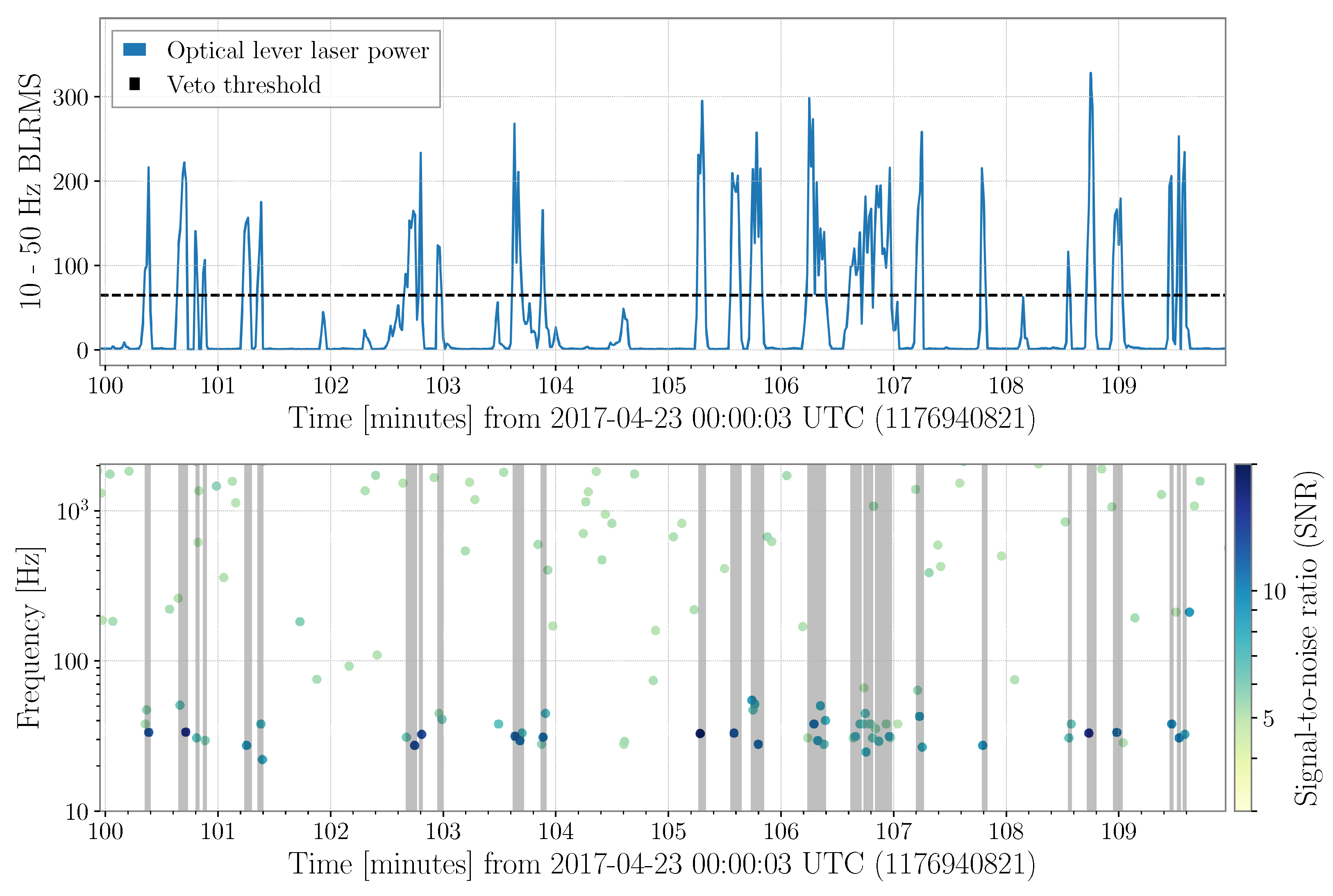
Figure 7.
An example of a gravitational-wave signal (GW190424_180648) with two different types of glitches also present nearby in the data. Event validation procedures were able to identify the source of both glitches as well as confirm that there was no evidence the gravitational-wave signal was an instrumental artifact. The source of one of the glitches was vibrations from an automated camera shutter that was inadvertently left running in one of the detector end stations [18] while the source of the second is light scattered off of the main laser beam path that reflects and then interferes with the main beam (referred to as “fast scattering”) [46]. This example highlights that it is possible to detect and analyze a gravitational-wave signal despite the presence of nearby glitches. Data plotted is from LIGO Livingston and accessed via GWOSC [90].
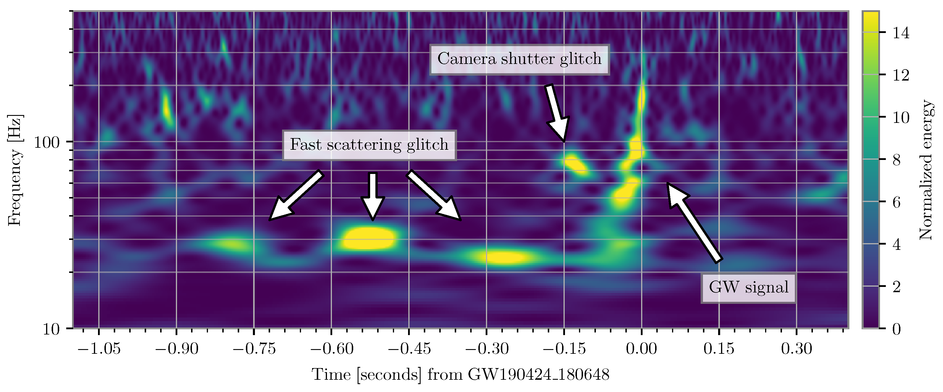
Figure 8.
An example of how continuous wave candidates (red dots) are validated based on lists of known lines in the strain data and a variety of signal consistency checks. The threshold for additional followup is shown with a black line. Candidates that are vetoed due to overlapping the known frequency of an instrumental line are marked with gray circles. Candidates that are vetoed because the amplitude of the signal is higher in one detector than expected for an astrophysical signal are marked with green triangles. Candidates that are only significant when considering half of the total analysis time are marked with blue squares. Reprinted figure with permission from [118]; Copyright 2018 by the American Physical Society.
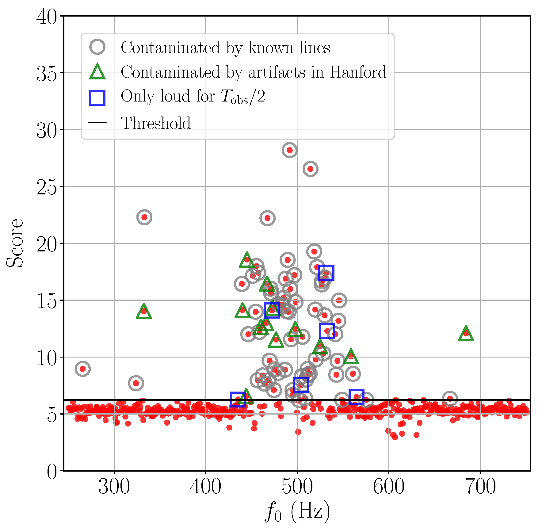
Figure 9.
A comparison of the amplitude spectral density (ASD) of the strain data at LIGO Hanford (H1) before (green) and after (blue) subtraction of broadband noise in O2. By using instrumental witnesses to known sources of noise, broadband noise between 80 and 1000 Hz was significantly reduced, as well as elimination of many narrow frequency band spectral artifacts caused by calibration lines and other instrumental factors. Figure is reproduced from [130]. © IOP Publishing. Reproduced with permission. All rights reserved.

Figure 10.
A demonstration of mitigating a glitch by modeling and subtracting the glitch with BayesWave [138,139,140]. (Left column): Spectrograms of whitened strain data from the LIGO Livingston detector before and after subtraction of the glitch. (Right column): Time series of the whitened strain before and after subtraction is plotted in blue, while the difference between the data before and after glitch subtraction is plotted in orange. After modeling and subtracting the glitch, the data are consistent with Gaussian noise. Plotted data are from [141].
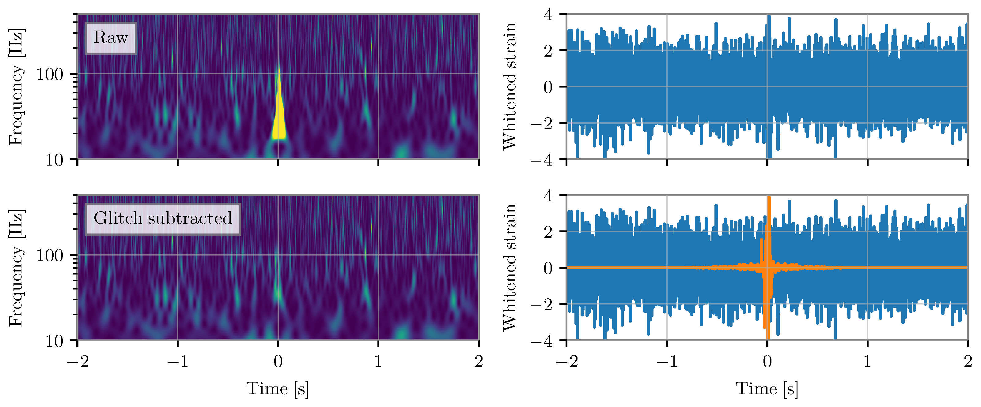
Figure 11.
A comparison of the use of gating and inpainting to mitigate a loud noise artifact in the data. Left column: Spectrograms of whitened strain data from the LIGO Livingston detector before mitigation, after mitigation with pre-whitening gating, and after mitigation with inpainting. Right column: Whitened strain time series for the same three cases. Both gating and inpainting methods mitigate the excess power from the instrumental artifact but inpainting introduces fewer artifacts and disturbs less of the time series. This improved mitigation comes at the cost of additional complexity in the method and the requirement that a specific PSD is used to analyze the data after inpainting. Plotted data are accessed from GWOSC [90].
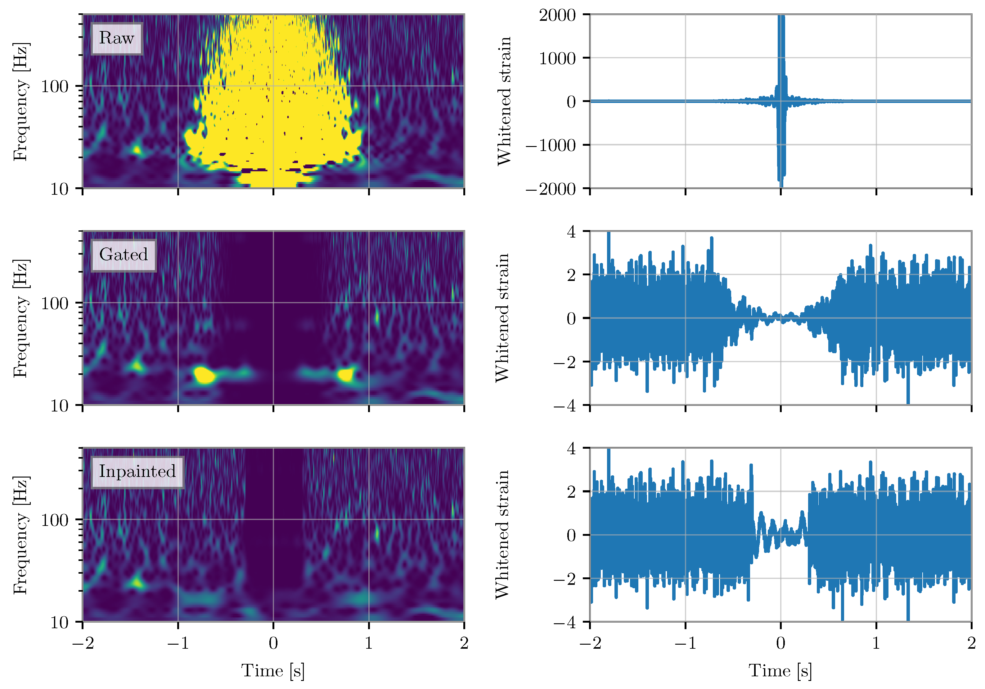
Publisher’s Note: MDPI stays neutral with regard to jurisdictional claims in published maps and institutional affiliations. |
© 2022 by the authors. Licensee MDPI, Basel, Switzerland. This article is an open access article distributed under the terms and conditions of the Creative Commons Attribution (CC BY) license (https://creativecommons.org/licenses/by/4.0/).
Share and Cite
MDPI and ACS Style
Davis, D.; Walker, M. Detector Characterization and Mitigation of Noise in Ground-Based Gravitational-Wave Interferometers. Galaxies 2022, 10, 12. https://doi.org/10.3390/galaxies10010012
AMA Style
Davis D, Walker M. Detector Characterization and Mitigation of Noise in Ground-Based Gravitational-Wave Interferometers. Galaxies. 2022; 10(1):12. https://doi.org/10.3390/galaxies10010012
Chicago/Turabian StyleDavis, Derek, and Marissa Walker. 2022. "Detector Characterization and Mitigation of Noise in Ground-Based Gravitational-Wave Interferometers" Galaxies 10, no. 1: 12. https://doi.org/10.3390/galaxies10010012
Note that from the first issue of 2016, this journal uses article numbers instead of page numbers. See further details here.