
Radiative Signatures of Parsec-Scale Magnetised Jets
by
 ,
,
Christian M. Fromm
1,2,*, 
Oliver Porth
1,
Ziri Younsi
1,
Yosuke Mizuno
1,
Mariafelica De Laurentis
1,
Hector Olivares
1 and
Luciano Rezzolla
1,3 1
Institut für Theoretische Physik, Goethe Universität, Max-von-Laue-Str. 1, D-60438 Frankfurt, Germany
2
Max-Planck-Institut für Radioastronomie, Auf dem Hügel 69, D-53121 Bonn, Germany
3
Frankfurt Institute for Advanced Studies, Ruth-Moufang-Strasse 1, 60438 Frankfurt, Germany
*
Author to whom correspondence should be addressed.
Galaxies 2017, 5(4), 73; https://doi.org/10.3390/galaxies5040073
Submission received: 18 September 2017
/
Revised: 1 November 2017
/
Accepted: 2 November 2017
/
Published: 6 November 2017
(This article belongs to the Special Issue Polarised Emission from Astrophysical Jets)
Abstract
:Relativistic jets are launched from the immediate vicinity of black holes and can reach kilo-parsec scales. During their evolution from the smallest to the largest scales, they encounter different physical conditions (e.g., ambient configurations and magnetic fields) which can modify their morphology and dynamics. Using state-of-the-art relativistic magneto-hydrodynamical simulations and ray-tracing algorithms, we model the dynamics of jets along with their radiation microphysics, investigating the impact of magnetisation on the jet dynamics and the observed emission. During the post-processing procedure we account for the properties of the observing array (sparse uv-plane) and the imaging algorithm, enabling a more direct comparison between simulations and ground-or space-based very-long-baseline interferometry (VLBI) observations. The different jet models can be distinguished from the reconstructed radio images.
1. Introduction
Relativistic jets are among the most powerful phenomena in the Universe. They are launched in the immediate vicinity of black holes and propagate as collimated flows up to kilo-parsec scales. According to our current understanding of relativistic jets, magnetic fields play a key role in their formation and propagation. However, the geometry and the magnitude of the magnetic field cannot be measured directly. Instead this information is imprinted in the observed electromagnetic emission generated from within the relativistic jet itself. Based on astronomical observations, the assumed dominant emission mechanism in relativistic jets is synchrotron radiation from relativistic particles gyrating around magnetic field lines. Very-long-baseline interferometry (VLBI) offers the unique capability of resolving the structure of relativistic jets and monitoring their temporal and spatial evolution. Due to the sparse sampling of the Fourier plane, it is challenging to investigate the underlying radiation microphysics (e.g., the number density of the relativistic particles and the magnetic field properties). By performing multi-frequency VLBI observations, estimates of the magnetic field can be extracted by computing the core-shift (i.e., the frequency-dependent position of the VLBI core—the observed apex of the jet), or by extracting the turnover frequency, , and turnover flux density, (e.g., [1,2,3]). To probe the effects of different jet configurations on the observed emission, special-relativistic magneto-hydrodynamical (SRMHD) simulations together with radiative transfer calculations can be used (e.g., [4,5,6]). The simulated radiative signatures can be employed to explain and interpret observed features in the VLBI images and single-dish spectra (see for example [7] for a case of shock–shock interaction in jets).
Throughout the paper we assume an ideal-fluid equation of state , where p is the pressure, the rest-mass density, the specific internal energy, and the adiabatic index [8]. In this work we use an adiabatic index of , which corresponds to a jet consisting of relativistic electrons and sub-relativistic protons.
2. Methods
2.1. SRMHD Simulations
For our simulations of relativistic jets we use the state-of-the-art code AMR-VAC [9,10] and solve the 1D time-dependent equations of SRMHD in cylindrical coordinates. For , the time-dependent 1D SRMHD solutions resemble the 2D steady-state structure of relativistic jets by substituting (see [11] for details). The 1D equations are evolved over 2000 time units. We use 400 cells in the radial direction with a resolution of 20 cells per jet radii. Thus, our numerical gird consists of cells, translating to a physical scale of . The setup at the jet nozzle follows the core-envelope solution of [12], and is characterised by the pressure, p, the co-moving magnetic field in azimuthal direction, , and the axial magnetic field, :
with : and : . In the above equations is the core radius, is the jet radius, and indicates the fraction of axial magnetic field in the jet sheath. The above profiles can be accompanied by any velocity and density profile. Again, we follow [11] and use for the bulk Lorentz factor:
where is the initial bulk Lorentz factor. For we obtain a constant bulk Lorentz Factor across the jet and an ambient medium at rest. The density profile is given by:
with the ambient medium density at the jet nozzle and the density ratio between the jet and the ambient medium. The pressure distribution in the ambient medium is modelled via a power law, , where the subscript 0 denotes values evaluated in the jet nozzle. In this work we investigate the influence of the magnetisation, , on the jet structure and on the non-thermal emission, selecting three different representative values for as , , and , while keeping the other model parameters fixed. Within the setup presented above, the different values for the magnetisation are realised by varying and while keeping the pressure constant. In Table 1 we list the initial parameters used for the simulations. Note that the approach presented above is only valid for v ~ c and leads to steady-state solutions which are comparable to the steady-state solutions of 2D SRMHD simulations.
2.2. Radiative Transfer Calculations and Synthetic Imaging
In order to compute the synchrotron emission from the SRMHD simulations we must reconstruct a non-thermal particle distribution. We follow the work of [5] and provide the basic expressions for the emission calculations below. We assume a power law distribution of relativistic particles:
with normalisation coefficient , spectral index s, and lower/upper electron Lorentz factor . The normalisation coefficient can be written as:
where is the thermal to non-thermal energy density, and the lower and upper electron Lorentz factor is given by:
In the equation above, is the thermal to non-thermal number density ratio and corresponds to the ratio between the electron Lorentz factors. Given the expressions for , , and , the coefficients for emission, , and absorption, , may be written as1:
where is the characteristic frequency, is the angle between the direction to the observer and the direction of the magnetic field, and , where is the electron charge. The value of depends on the orientation of the magnetic field (see [5] for details), and the total intensity along a ray with path length in the observer’s frame is obtained by solving the transport equation using the co-moving emission and absorption coefficients:
with Doppler factor , is the velocity of the jet and is the viewing angle. Finally the observed flux density, taking cosmological corrections into account, is given by:
In the above equation, z corresponds to the redshift, to the luminosity distance, and and to the resolution of the detector frame. In Table 2 we list the emission and scaling parameters (required for the conversion from code units to physical units) used for calculation of the non-thermal radiation. The ray-tracing is performed on a 3D Cartesian grid (x, y, z) created by a Delaunay triangulation of the 2D cylindrical (r, z) SRMHD simulation. A typical 3D grid consists of cells. In the post-processing of the ray-traced images we assume a typical Very Long Baseline Array (VLBA) experiment (i.e., only a fraction of the total observation time—here 10 min per scan—is spent on the source). For the VLBA antennas we apply a system temperature of between 55 K and 65 K, a diameter of 25 m, and a system efficiency of between 50% and 70%. The ray-traced image is Fourier-transformed and sampled with the uv-coordinates of the antennas given their location and the time of the observations. For each antenna, thermal noise (depending on the system temperature) is taken into account. The obtained visibilities are read into DIFMAP [13] and imaged via the CLEAN algorithm [14].
3. Results
The results of the SRMHD simulations using the values listed in Table 1 are presented in Figure 1, showing the 2D distribution of the pressure for three different initial magnetisations (left panel) and the 2D distribution of the magnetisation for different initial values (right panel). In each panel, the initial magnetisation increases from left to right from to and the solid black lines indicate the jet boundary, with the thin black lines corresponding to stream lines along the jet. Independent of the magnetisation all jet models show oscillations of the jet boundary, i.e., an expansion and collimation of the jet which can be explained by the adjustment of the jet to the decreasing pressure ambient medium (e.g., [15]). However, with increasing magnetisation the wavelength of the oscillation is decreasing and recollimation shocks become weaker (see the left panel in Figure 1). At the same time, the regions of highest magnetisation along the jet are moving towards the jet axis with increased initial magnetisation (see the right panel in Figure 1).
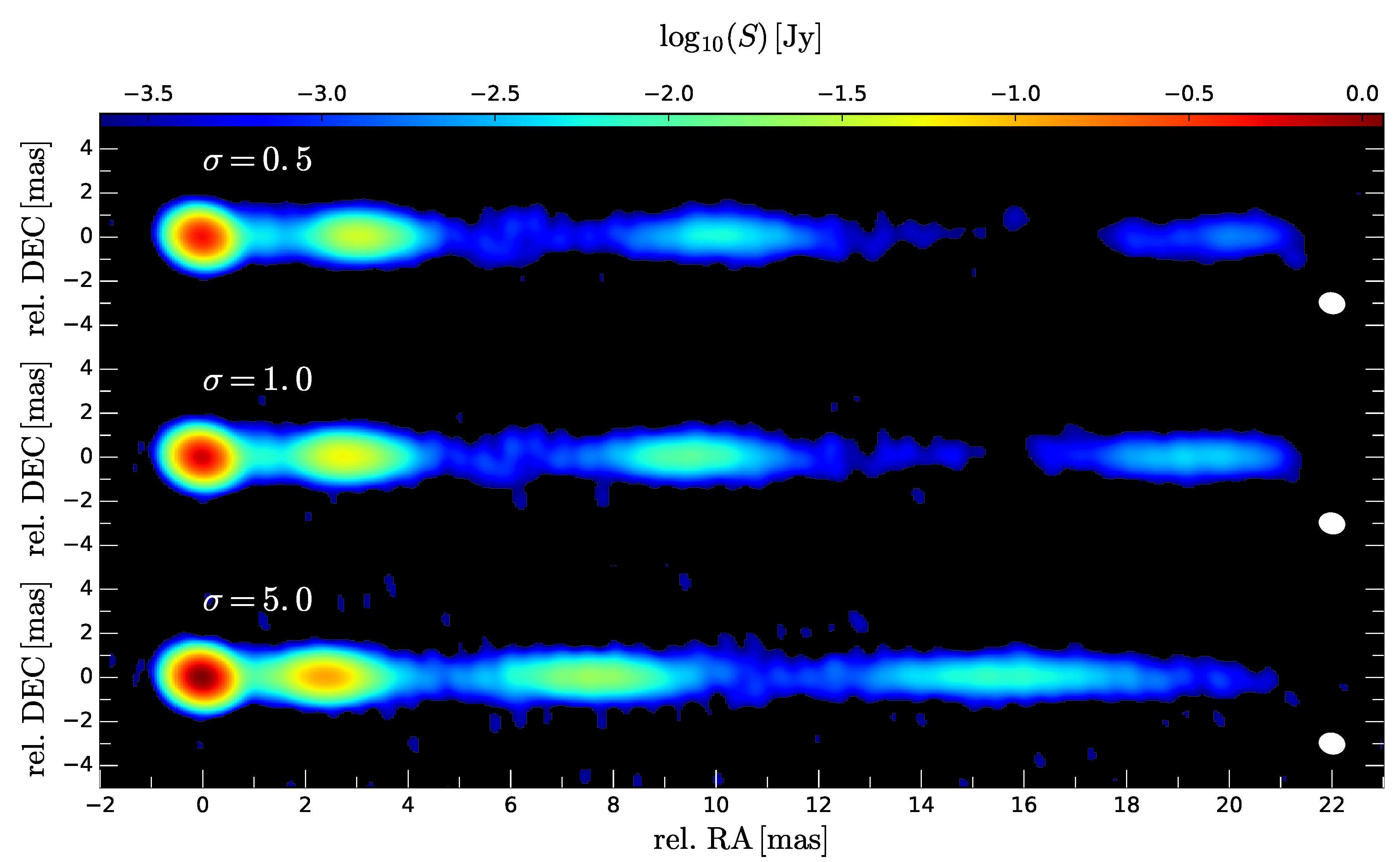
In Figure 2 we present the results of our radiative transfer calculations and synthetic imaging. From top to bottom we show the 15 GHz VLBA radio maps for , , and . The convolving beam for the observations is plotted in the lower right corner of each image. The bright region at is the jet nozzle, and the additional regions of enhanced and reduced emission correspond to the oscillation of the jet boundary. Depending on the magnetisation, the regions of increased emission appear closer (high magnetisation) or further downstream (low magnetisation) from the jet nozzle. Furthermore, the emission along the jet is decreasing faster in the low magnetisation case than in the high magnetisation case.
4. Discussion and Conclusions
In this work we investigated the impact of the initial magnetisation on the structure and the observed emission of relativistic jets. The results of the SRMHD simulations show that the wavelength of the jet boundary oscillation increases with magnetisation. This effect can be understood in terms of the magneto-sonic speed and the corresponding Mach number. An increase in the magnetisation leads to faster magneto-sonic waves (reduced Mach numbers), and it takes less time for the waves to cross the jet transversally. As a result, magnetised jets are more collimated and show a shorter wavelength in the oscillation of the jet boundary as compared to less magnetised jets. In addition, the increase of the magnetisation induces a higher magnetic tension and the formation of recollimation shocks is suppressed (e.g., [11,16]).
For the comparison with VLBI observations, we computed the non-thermal emission and created synthetic radio maps. The trend seen in these maps can be summarised as follows: the observed emission is increasing with increasing magnetisation. The collimation of the jet boundary leads to an amplification of the density, pressure, and magnetic field, which translates into an increase in the emission. On the other hand, in the expansion regions the thermodynamic parameters decrease, causing a reduction in the non-thermal emission. Since the jets are embedded in a decreasing-pressure atmosphere, the emission decreases with distance from the jet nozzle. Due to the sparse sampling of the uv-plane and the noise limitation of the VLBA (at 15 GHz with 10 min on-source integration time 2), some of the outermost expansion regions cannot be detected and gaps between the collimation regions appear (see the case at x ).
Within our model, strongly magnetised jets appear more collimated (no gaps between local flux density maxima) and exhibit a larger number of enhanced emission regions than weakly magnetised jets. However, a more detailed analysis of the synthetic radio maps is required to investigate the observational differences between weakly- and strongly-magnetised jets.
Acknowledgments
Support comes from the ERC Synergy Grant “BlackHoleCam—Imaging the Event Horizon of Black Holes” (Grant 610058). ZY acknowledges support from an Alexander von Humboldt Fellowship.
Author Contributions
Christian M. Fromm and Ziri Younsi: Emission calculations and synthetic imaging; Oliver Porth, Yosuke Mizuno and Hector Olivares: SRMHD simulations; Mariafelica de Laurentis and Luciano Rezzolla: Critical contributions for physical interpretation of the simulation results.
Conflicts of Interest
The authors declare no conflict of interest.
References
- Marcaide, J.M.; Shapiro, I.I. High precision astrometry via very-long-baseline radio interferometry: Estimate of the angular separation between the quasars 1038+528A and B. Astroph. J. 1983, 88, 1133–1137. [Google Scholar] [CrossRef]
- Lobanov, A.P. Ultracompact jets in active galactic nuclei. Astron. Astrophys. 1998, 330, 79–89. [Google Scholar]
- Fromm, C.M.; Ros, E.; Perucho, M.; Savolainen, T.; Mimica, P.; Kadler, M.; Lobanov, A.P.; Zensus, J.A. Catching the radio flare in CTA 102. III. Core-shift and spectral analysis. Astron. Astrophys. 2013, 557, A105. [Google Scholar] [CrossRef]
- Gómez, J.L.; Marti, J.M.A.; Marscher, A.P.; Ibanez, J.M.A.; Marcaide, J.M. Parsec-Scale Synchrotron Emission from Hydrodynamic Relativistic Jets in Active Galactic Nuclei. Astrophys. J. Lett. 1995, 449, L19. [Google Scholar] [CrossRef]
- Mimica, P.; Aloy, M.-A.; Agudo, I.; Martí, J.M.; Gómez, J.L.; Miralles, J.A. Spectral Evolution of Superluminal Components in Parsec-Scale Jets. Astrophys. J. 2009, 696, 1142–1163. [Google Scholar] [CrossRef]
- Porth, O.; Fendt, C.; Meliani, Z.; Vaidya, B. Synchrotron Radiation of Self-collimating Relativistic Magnetohydrodynamic Jets. Astrophys. J. 2011, 737, 42. [Google Scholar] [CrossRef]
- Fromm, C.M.; Perucho, M.; Mimica, P.; Ros, E. Spectral evolution of flaring blazars from numerical simulations. Astron. Astrophys. 2016, 588, A101. [Google Scholar] [CrossRef]
- Rezzolla, L.; Zanotti, O. Relativistic Hydrodynamics; Oxford University Press: Oxford, UK, 2013; ISBN-10 0198528906. [Google Scholar]
- Keppens, R.; Meliani, Z.; van Marle, A.J.; Delmont, P.; Vlasis, A.; van der Holst, B. Parallel, grid-adaptive approaches for relativistic hydro and magnetohydrodynamics. J. Comput. Phys. 2011, 231, 718–744. [Google Scholar] [CrossRef]
- Porth, O.; Xia, C.; Hendrix, T.; Moschou, S.P.; Keppens, R. MPI-AMRVAC for Solar and Astrophysics. Astrophys. J. Suppl. Ser. 2014, 214, 4. [Google Scholar] [CrossRef]
- Komissarov, S.S.; Porth, O.; Lyutikov, M. Stationary relativistic jets. Comput. Astrophys. Cosmol. 2015, 1, 9. [Google Scholar] [CrossRef]
- Komissarov, S.S. Numerical simulations of relativistic magnetized jets. Mon. Not. R. Astron. Soc. 1999, 308, 1069–1076. [Google Scholar] [CrossRef]
- Shepherd, M.C. Difmap: An Interactive Program for Synthesis Imaging. Astron. Data Anal. Softw. Syst. VI 1997, 125, 77. [Google Scholar]
- Högbom, J.A. Aperture Synthesis with a Non-Regular Distribution of Interferometer Baselines. Astron. Astrophys. Suppl. 1974, 15, 417. [Google Scholar]
- Falle, S.A.E.G. Self-similar jets. Mon. Not. R. Astron. Soc. 1991, 250, 581–596. [Google Scholar] [CrossRef]
- Mizuno, Y.; Gómez, J.L.; Nishikawa, K.-I.; Meli, A.; Hardee, P.E.; Rezzolla, L. Recollimation Shocks in Magnetized Relativistic Jets. Astrophys. J. 2015, 809, 38. [Google Scholar] [CrossRef]
| 1. | Dashed values indicate the co-moving system. |
| 2. |
Figure 1.
2D distribution of the pressure (left panel) and magnetisation (right panel) for different initial magnetisations (for details see text).
Figure 1.
2D distribution of the pressure (left panel) and magnetisation (right panel) for different initial magnetisations (for details see text).
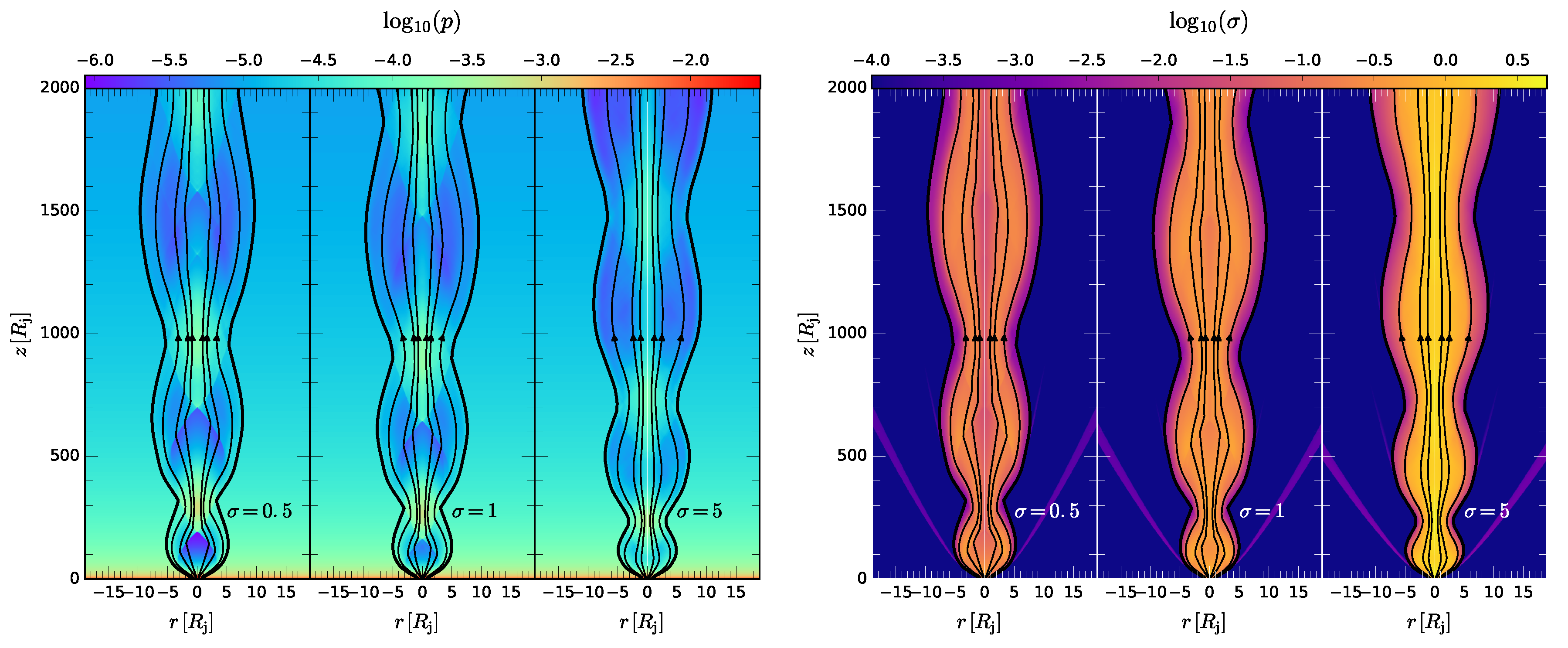
Figure 2.
Radio maps (15 GHz) using the Very Long Baseline Array (VLBA) as the observing array for different initial magnetisations (indicated in top left corner). The convolving beam of is plotted in the lower right corner.
Figure 2.
Radio maps (15 GHz) using the Very Long Baseline Array (VLBA) as the observing array for different initial magnetisations (indicated in top left corner). The convolving beam of is plotted in the lower right corner.

Table 1.
Initial parameters for the special-relativistic magneto-hydrodynamical (SRMHD) in code units (varying values in bold face).
Table 1.
Initial parameters for the special-relativistic magneto-hydrodynamical (SRMHD) in code units (varying values in bold face).
| 0.37 | 1.0 | 0.14 | 1.85 | 0.95 | 8.0 | 1.0 | 0.01 | 1.0 | 13/9 | 0.5 |
| 0.37 | 1.0 | 0.19 | 1.00 | 0.95 | 8.0 | 1.0 | 0.01 | 1.0 | 13/9 | 1.0 |
| 0.37 | 1.0 | 0.34 | 0.30 | 0.95 | 8.0 | 1.0 | 0.01 | 1.0 | 13/9 | 5.0 |
Table 2.
Emission parameters used for the calculation of the non-thermal radiation.
| s | z | ||||||
|---|---|---|---|---|---|---|---|
| 5 | 0.3 | 1.0 | 2.2 | 1.0 |
© 2017 by the authors. Licensee MDPI, Basel, Switzerland. This article is an open access article distributed under the terms and conditions of the Creative Commons Attribution (CC BY) license (http://creativecommons.org/licenses/by/4.0/).
Share and Cite
MDPI and ACS Style
Fromm, C.M.; Porth, O.; Younsi, Z.; Mizuno, Y.; De Laurentis, M.; Olivares, H.; Rezzolla, L. Radiative Signatures of Parsec-Scale Magnetised Jets. Galaxies 2017, 5, 73. https://doi.org/10.3390/galaxies5040073
AMA Style
Fromm CM, Porth O, Younsi Z, Mizuno Y, De Laurentis M, Olivares H, Rezzolla L. Radiative Signatures of Parsec-Scale Magnetised Jets. Galaxies. 2017; 5(4):73. https://doi.org/10.3390/galaxies5040073
Chicago/Turabian StyleFromm, Christian M., Oliver Porth, Ziri Younsi, Yosuke Mizuno, Mariafelica De Laurentis, Hector Olivares, and Luciano Rezzolla. 2017. "Radiative Signatures of Parsec-Scale Magnetised Jets" Galaxies 5, no. 4: 73. https://doi.org/10.3390/galaxies5040073
Note that from the first issue of 2016, this journal uses article numbers instead of page numbers. See further details here.