Characterising the Long-Term Variability of Blazars in Leptonic Models

Abstract

Most research on blazar variability focuses on individual flares to explain acceleration and radiation mechanisms and improve on current models. These short-time events (being minutes, hours, or days) might not be representative of the underlying mechanisms causing small-amplitude variability and/or continuous emission which is present most of the time. We will therefore investigate long-term (months to years) variability of blazar emission in the framework of current leptonic blazar models. For this purpose, we introduce generated time-dependent parameter variations which are based on typical Power Spectral Densities (PSDs) associated with the variability of accretion flows. The PSDs from the resulting light curves are analyzed and compared to one another, as well as the PSD of the input variation. Correlations between light curves are also investigated to aid identification of characteristic variation patterns associated with leptonic models.

1. Introduction

Blazars are a class of active galactic nuclei (AGN) in which the collimated relativistic jets are aligned close to our line of sight. Their spectral energy distributions (SED) are characterized by two distinct non-thermal peaks, the low-energy peak ranging from radio to ultraviolet (UV) or soft X-rays, and the high-energy peak ranging from X-rays to $\gamma$-rays, in some cases up to TeV energies.

There are mainly two different models that have been developed and which can successfully explain the emission of most blazars—leptonic and hadronic models. Relativistic electrons and positrons generate synchrotron radiation, which is the cause of the low-energy peak in both models. The high-energy peak, however, is the result of Inverse Compton (IC) scattering of low-energy photons in the leptonic model, while in the hadronic model it is considered to be dominated by synchrotron emission from protons and/or photopion production and subsequent electromagnetic cascades. For a more thorough review of both models, please consult [1].

Variability over the whole electromagnetic spectrum is a known characteristic of blazar emission. The time-scales of these rapid changes can be as short as a few minutes [2,3]. Most research on variability focuses on short-lived events (hours to days) such as flares, in order to constrain models (e.g., [4]). This approach does not consider long-term variability that is always present [5]. This motivates an investigation into long-term variability (months to years) to study the underlying causes of variability.

The exact causes of long-term variability are unknown, but multi-wavelength light curve Power Spectral Densities (PSDs) have shown it to be characterized by red noise [5], similar to the high-frequency variability in X-ray binary systems [6,7] which is associated with accretion.

This trend, along with our current understanding of leptonic blazar emission, is used to construct a method of simulating variability by assuming the variations to be variations of emission region parameters with predetermined stochastic PSDs. The variability patterns that follow from these variations are then analysed. This work is done numerically much like that of [8], but similar analytic work has been done by [9,10] in which the variability was investigated in Fourier space for similar causes of variability.

The leptonic model and simulation of variability is discussed in Section 2. The results for the variations of different parameters and a discussion of the differences are presented in Section 3. In Section 4, we give a summary and conclusions.

2. Model and Setup

We employed the one-zone time-dependent leptonic model developed by [11], adapted for long-term variations [12]. A representative test case that can be adequately described by the leptonic model is used.

Table 1. Baseline model parameters used in the leptonic code, similar to that of [12].

Definition	Value
Magnetic field of the emission region	3.70 G
Blob radius	$2.50\times {10}^{16}$ cm
Ratio of the acceleration to escape time-scales	1.00
Escape time-scale	$10.0R/c$
Redshift to the source	1.037
Minimum Lorentz factor for the electron injection spectrum	$1.0\times {10}^1$
Maximum Lorentz factor for the electron injection spectrum	$3.0\times {10}^3$
Bulk Lorentz factor for the blob	35.0
Observing angle relative to the axis of the black hole jet	$2.86\times {10}^{-2}$ rad
Electron injection index	2.4
Co-moving injection luminosity for the electron spectrum	$2.40\times {10}^{43}$ erg/s
Mass of the super-massive black hole	$8.5\times {10}^8{M}_{\odot }$
Eddington ratio	$3.50\times {10}^{-1}$
Initial location of the blob along jet axis	$6.50\times {10}^{17}$ cm
Radius of the broad line region (BLR)	$6.70\times {10}^{17}$ cm
Effective temperature of the BLR	$5.0\times {10}^4$ K
Effective luminosity of the BLR	$4.14\times {10}^{45}$ erg/s

provides the base parameters for this test case.

The steady-state SED with the baseline parameters of Table 1 is shown in Figure 1. It is clear that in this case, the synchrotron, accretion disc emission, and IC scattering of the broad line region (BLR) photons are the dominant components that produce the characteristic double-peaked non-thermal spectrum. The shaded areas indicate the energy ranges used to extract light curves from the model: 20 MeV–300 GeV [$\gamma$-rays], 0.2–10 keV [X-rays], optical R-band, 73 MHz–50 GHz [radio emission].

In this setup, we generate a stochastic time-dependent variation as the variation of one parameter in the emission region.

The method of [13] was used to generate the stochastic time-dependent variations by assuming a PSD spectrum. The seed PSD spectrum, $S\left(f\right)$, was chosen as a simple power law with index $\alpha$, which can often be associated with the PSD spectra of X-ray binaries; thus, $S\left(f\right)=f^{-\alpha }$.

The method calculates a periodogram (Fourier inverse of time-series) for a given PSD spectrum and involves obtaining complex numbers from normally distributed random variables that depend on the spectrum. The computation is thus:

$$P\left(f\right)=\mathcal{N}(0,\frac{1}{2}S\left(f\right))+i\mathcal{N}(0,\frac{1}{2}S\left(f\right))$$

(1)

where $P\left(f\right)$ is the periodogram, and $\mathcal{N}(\overline{x},{\sigma }^2)$ a normally distributed random variable for mean $\overline{x}$ and variance ${\sigma }^2$. The PSD is simply ${\left|P\left(f\right)\right|}^2$. The time-series (variation) is recovered by taking the Fast Fourier Transform (FFT) of $P\left(f\right)$:

$$V\left(t\right)=\mathrm{FFT}\left[P\right(f\left)\right]$$

(2)

Furthermore, the time-series is manipulated to be suitable for parameter ranges of the model by adding or multiplying with constants. This does not affect the power law index of the PSD in any way. The properties in the emission region we chose to vary were the electron injection luminosity, magnetic field strength, and electron spectral index in separate realisations of the simulation. A typical variation generated by this method for an arbitrarily sized time step is shown in Figure 2.

Light curves produced by the leptonic model for the given variation were analysed. PSDs were calculated by FFT to be compared to the input variation PSD and different variations.

Cross-correlations between light curves of different frequencies were also calculated to probe correlations and possible time lags between the variability in different energy bands.

In this work, we fixed the time-step size of the variation in the jet frame to $\Delta t=2$ h, and 4000 steps for a total duration of 8000 h. Due to Doppler boosting, the total duration was shortened to 456 h in the observer’s frame (Figure 3).

3. Results and Discussion

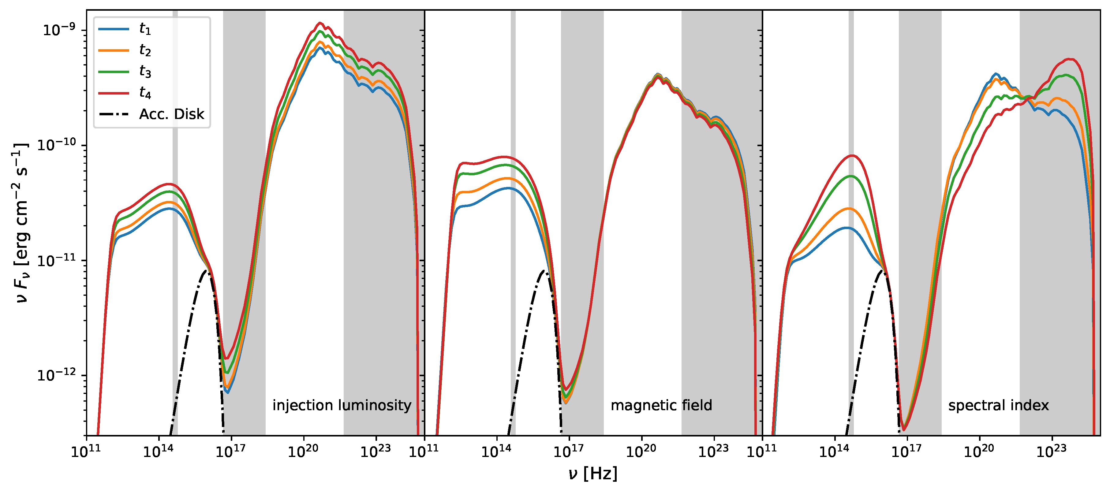
The light curves resulting from the variation shown in Figure 2 are presented in Figure 3. The evolution of the SED for the variation of the different parameters are also shown in Figure 4. Clear differences between the different varied parameters are apparent. The synchrotron emission is strongly synchrotron-self-absorbed at the chosen radio frequencies. Therefore, the radio light curves show distinctly different behaviour from all of the other wavebands.

In the case of injection luminosity variations, we see a synchronised rise and fall of flux over all wavelengths (left panel) with the average flux normalised optical and $\gamma$-ray light curves practically being identical on hour time-scales. A delay in X-rays with respect to $\gamma$-rays is also apparent.

The sensitivity of synchrotron radiation with respect to magnetic field variations is seen with the high variability of radio and optical wavelengths (middle panel). The increased cooling efficiency of stronger magnetic fields is apparent in the anti-correlation in $\gamma$-rays, which is IC-dominated. The X-rays have a weak correlation to the optical due to a significant contribution from synchrotron self-Compton (SSC) scattering.

The spectral index variation (right panel) for constant injection luminosity redistributes electrons from high to low energies and vice versa. Consequently, we expect correlated optical and $\gamma$-rays produced by high-energy electrons, and anti-correlated with X-rays produced by low-energy electrons.

3.1. Power Spectral Densities

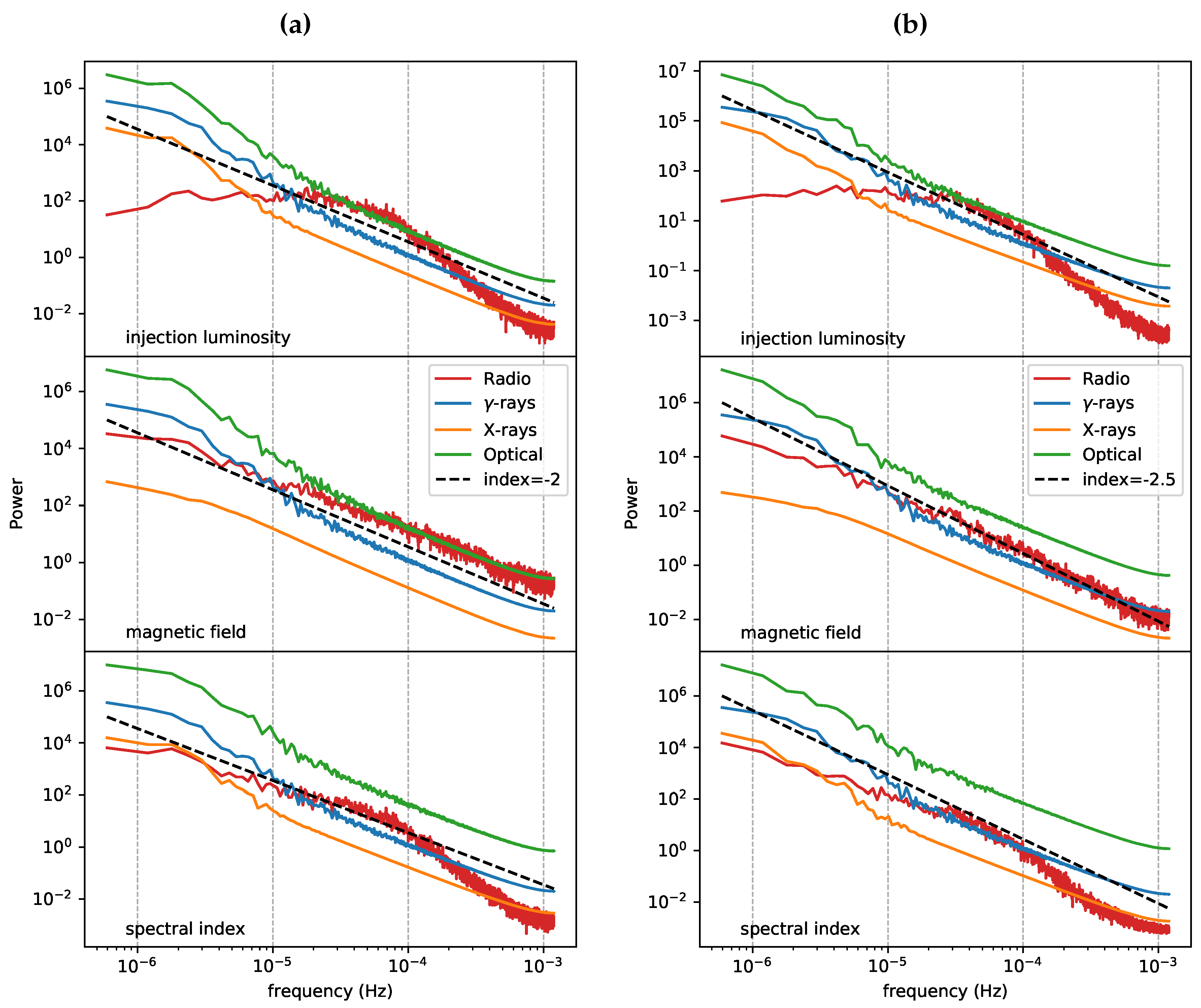
To eliminate noise, ten realisations for the same seed index $\alpha$ were used to produce average light curve PSDs. The results are presented in Figure 5 compared to the seed power law spectrum.

For $\alpha =2.0$, the PSDs follow the seed index closely for all wavelengths across all variations except for the radio where absorption effects are significant. The variability in the optical, X-ray, and $\gamma$-ray light curves is much smoother than the input variation itself, and therefore the resulting PSDs are also smoother than the input PSD. This smoothness is an effect of the finite cooling time-scales and light travel time effects demonstrated by [8].

For $\alpha =2.5$ the PSDs has a noticeable deviation from the seed index compared to the case of $\alpha =2.0$. The indices of the light curve PSDs are harder than the seed in all variations. The X-ray PSD for the magnetic variation also seems to have deviated slightly from its optical and $\gamma$-ray counterparts at low frequencies, contrary to the case of $\alpha =2.0$.

3.2. Cross-Correlations

The cross-correlations allow us to quantify correlations and possible time lags between variability in different frequency bands. Figure 6 shows the cross-correlation coefficients of the classical correlation function [14] for the different variations. We see that the $\gamma$-ray and optical wavelengths show almost perfect correlation/anti-correlation each time and the optical lagging behind the $\gamma$-rays by 3.5 min, the duration of a time step in the observer’s frame. Figure 7 illustrates this short time lag. This is an indication that these light curves are produced by electrons sharing a common energy range. Due to this small delay, further optical correlations are not shown for clarity.

The correlation functions for the injection luminosity variation light curves show almost perfect correlations, with some time lags between optical, X-rays, and $\gamma$-rays. The time lags are indicative of different cooling time-scales; that is, longer cooling time-scales for the low-energy electron population producing X-rays (lags behind $\gamma$-rays and optical) while shorter for the high-energy population producing optical and $\gamma$-rays.

The magnetic field and BLR co-moving energy densities govern the cooling rate and ratio of fluxes between the synchrotron and external IC/BLR components. This is seen in the anti-correlation between $\gamma$-rays and optical bands for magnetic field variations. Stronger magnetic fields are more efficient at cooling electrons, which reduces high-energy electrons for IC scattering. The weak anti-correlation between $\gamma$-rays and X-rays, i.e., the correlation between optical and X-rays, is especially interesting. This can be attributed to significance of the SSC and external IC/BLR components present in the X-ray range (Figure 1). The decrease in IC/BLR flux is met with an increase in SSC when magnetic fields are increased.

The strong correlation of $\gamma$-rays and optical for the spectral index variation can again be attributed to the high-energy electron population producing radiation in both these bands. The anti-correlation of X-rays with $\gamma$-rays (and therefore also optical) is due to the low-energy electrons that are responsible for producing X-rays. A spectral index softening results in a loss of high-energy electrons versus a gain in the low-energy population.

4. Summary and Conclusions

In this paper, we presented a method of modelling variability by producing a variation to be used as input to a time-dependent leptonic emission model for blazars that produce variable light curves. Evidence was presented that multi-wavelength light curve PSDs (optical, X-ray, and $\gamma$-rays) follow a steady index between temporal frequencies between ${10}^{-5}$ and ${10}^{-3}$ Hz which matches the input index in the case of $\alpha =2.0$.

Cross-correlations are an effective tool for rigorous distinction between variations of different properties of the emission region. They can also provide valuable insight into the sensitivity of models to certain changes in parameters. For well-sampled observations, one can expect that this would help with identification of the cause of variability, even if the variability progenitor is unknown.

This work has shown that investigations into long-term variability are a promising endeavour. Future prospects include expanding on parameters investigated, increasing frequency range and/or resolution, investigations with more complex seed PSDs, and comparison to observational blazar data, among others. It can be a useful tool to constrain models and identify the underlying mechanisms responsible for the characteristic variability in blazars.

References

- Boettcher, M.; Harris, D.E.; Krawczynski, H. Relativistic Jets from Active Galactic Nuclei; Wiley: Berlin, Germany, 2012. [Google Scholar]
- Aharonian, F.; Akhperjanian, A.G.; Bazer-Bachi, A.R.; Behera, B.; Beilicke, M.; Benbow, W.; Berge, D.; Bernlöhr, K.; Boisson, C.; Bolz, O.; et al. An Exceptional Very High Energy Gamma-Ray Flare of PKS 2155-304. Astrophys. J. 2007, 664, L71–L74. [Google Scholar] [CrossRef] [Green Version]
- Aharonian, F.; Akhperjanian, A.G.; Anton, G.; Barres de Almeida, U.; Bazer-Bachi, A.R.; Becherini, Y.; Behera, B.; Benbow, W.; Bernlöhr, K.; Boisson, C.; et al. Simultaneous multiwavelength observations of the second exceptional γ-ray flare of PKS 2155-304 in July 2006. Astron. Astrophys. Suppl. 2009, 502, 749–770. [Google Scholar] [CrossRef]
- Diltz, C.; Böttcher, M. Leptonic and Lepto-Hadronic Modeling of the 2010 November Flare from 3C 454.3. Astrophys. J. 2016, 826, 54. [Google Scholar] [CrossRef]
- Goyal, A.; Stawarz, Ł.; Zola, S.; Marchenko, V.; Soida, M.; Nilsson, K.; Ciprini, S.; Baran, A.; Ostrowski, M.; Wiita, P.J.; et al. Stochastic Modeling of Multiwavelength Variability of the Classical BL Lac Object OJ 287 on Timescales Ranging from Decades to Hours. Astrophys. J. 2018, 863, 175. [Google Scholar] [CrossRef]
- Van der Klis, M. Rapid aperiodic variability in X-ray binaries. In X-Ray Binaries (A 97-42726 11-90); Cambridge Astrophysics Series; Cambridge University Press: Cambridge, UK; New York, NY, USA, 1997; pp. 252–307. [Google Scholar]
- Cui, W. Temporal X-ray Properties of Galactic Black Hole Candidates: Observational Data and Theoretical Models. In High Energy Processes in Accreting Black Holes; Poutanen, J., Svensson, R., Eds.; Astronomical Society of the Pacific Conference Series; Astronomical Society of the Pacific (ASP): San Franscisco, CA, USA, 1999; Volume 161, p. 97. [Google Scholar]
- Mastichiadis, A.; Petropoulou, M.; Dimitrakoudis, S. Mrk 421 as a case study for TeV and X-ray variability in leptohadronic models. Mon. Not. R. Astron. Soc. 2013, 434, 2684–2695. [Google Scholar] [CrossRef] [Green Version]
- Finke, J.D.; Becker, P.A. Fourier Analysis of Blazar Variability. Astrophys. J. 2014, 791, 21. [Google Scholar] [CrossRef]
- Finke, J.D.; Becker, P.A. Fourier Analysis of Blazar Variability: Klein-Nishina Effects and the Jet Scattering Environment. Astrophys. J. 2015, 809, 85. [Google Scholar] [CrossRef]
- Diltz, C.; Böttcher, M. Time dependent leptonic modeling of Fermi II processes in the jets of flat spectrum radio quasars. J. High Energy Phys. 2014, 1, 63–70. [Google Scholar] [CrossRef] [Green Version]
- Zacharias, M.; Böttcher, M.; Jankowsky, F.; Lenain, J.P.; Wagner, S.J.; Wierzcholska, A. Cloud Ablation by a Relativistic Jet and the Extended Flare in CTA 102 in 2016 and 2017. Astrophys. J. 2017, 851, 72. [Google Scholar] [CrossRef] [Green Version]
- Timmer, J.; Koenig, M. On generating power law noise. Astron. Astrophys. Suppl. 1995, 300, 707. [Google Scholar]
- Oppenheim, A.V.; Schafer, R.W. Digital Signal Processing/Alan V. Oppenheim Ronald W. Schafer; Prentice-Hall: Englewood Cliffs, NJ, USA, 1975; p. xiv. 585p. [Google Scholar]