Abstract
We have used the varying physical constant approach to resolve the flatness problem in cosmology. Friedmann equations are modified to include the variability of speed of light, gravitational constant, cosmological constant, and the curvature constant. The continuity equation obtained with such modifications includes the scale factor-dependent cosmological term as well as the curvature term, along with the standard energy-momentum term. The result is that as the scale factor tends to zero (i.e., as the Big Bang is approached), the universe becomes strongly curved rather than flatter and flatter in the standard cosmology. We have used the supernovae 1a redshift versus distance modulus data to determine the curvature variation parameter of the new model, which yields a better fit to the data than the standard ΛCDM model. The universe is found to be an open type with a radius of curvature , where is the redshift, is the current speed of light, and is the Hubble constant.
PACS:
98.80.-k; 98.80.Es; 98.62.Py
1. Introduction
While the Big-Bang cosmology has been successful in explaining most observables of the universe, and has become arguably the most accepted theory since the discovery of microwave background in 1964 by Penzias and Wilson [1], the inflation phenomenon proposed by Guth in 1981 [2,3,4] as explanation for the flatness, horizon, and magnetic monopole problems remains rather contentious. Within the purview of the Big Bang, several alternatives have been suggested to explain one or more of these problems. We will mention only a few here to give a flavor of the alternatives proposed, as our intent is not to review the field, but rather to explore if the recently proposed variable constants approach [5] can resolve the flatness problem, especially since the approach was able to resolve three astrometric anomalies and fit the SNe Ia redshift data better than the standard CDM model.
An early review of the inflationary universe was written by Olive in 1990 [6], and an easy textbook description was provided in chapter 10 by Ryden in 2017 [7]. Levine and Freese in 1993 [8] attempted a possible solution to the horizon problem using the so-called MAD (massively aged and detained) approach in the massless scalar theory of gravity. Their approach is based on the time-dependent Planck mass without the dominance of dark energy that is pivotal in the inflationary cosmology. Hu, Turner, and Weinberg [9] studied the dynamical solutions to the horizon and flatness problems, and showed that in the context of scalar-tensor theories, the time-varying Planck mass cannot lead to a solution of the horizon problem. They also pointed out that there is an apparent paradox in discussing the horizon problem in the context of the Friedmann–Robertson–Walker (FRW) model, which has been developed assuming the universe to be isotropic and homogeneous. While the modeling of a generally inhomogeneous and anisotropic universe is very difficult, and any interpretation of solutions therefrom is even more difficult [10,11], an easier approach is to consider the perturbation of the FRW model and explore if the inhomogeneity created by such perturbations is contained to the level of observations. One could further question that even if the universe was causally connected, and thus homogeneous and isotropic during the inflationary epoch, what kept the inhomogeneities from developing from the time inflation ended to the time when cosmic microwave background (CMB) radiation was emitted yrs when the universe was no longer causally connected? More recently, Singal has asserted that based on theories developed using FRW metric, which a priori assume the universe to be homogeneous and isotropic, one cannot use homogeneity and flatness problems in support of inflation [12].
While the horizon problem can be stated as ‘why there is a high level of isotropy and homogeneity observed in CMB data when most of the universe could not possibly be causally connected’, the flatness problem seeks to answer: ‘Why is the energy density of the universe so close to the critical energy density (the latter, being the energy density, assuming the curvature term to be absent in the FRW model, i.e. the universe to be flat) today, meaning that the universe is almost flat today—and why it was even flatter in the past?’ [7]. This means that if we write the ratio of the energy density to its critical energy density as , then what we get in the FRW model is that if we have, say now at time , then at Planck, time , !
Barrow and Magueijo have addressed the flatness and cosmological constant () problem with an evolutionary speed of light theory in which the speed of light falls off with increasing cosmic time [13,14]. Berera, Gleiser, and Ramos presented a quantum field theory warm inflation model for solving the horizon and flatness problem wherein in the realm of the elementary dynamics of particle physics, cosmological scale factor trajectories that originate in the radiation-dominated epoch enter an inflationary epoch, and finally exit back to the radiation-dominated epoch, with significant radiation throughout the evolution [15]. Lake has shown through a complete integration of Friedmann equations that for , there exist nonflat FRW models for which throughout the entire history of the universe [16]. Fathi, Jalalzadeh, and Moniz used quantum cosmology, based on the application of the de Broglie–Bohm formulation in quantum mechanics to a spatially closed universe comprising radiation and matter perfect fluids, to show that expanding the classical universe can emerge from an oscillating quantum universe without singularity and without the horizon or flatness problems [17]. Using anisotropic scaling, which leads to a novel mechanism of generating scale-invariant cosmological perturbations and resolution of the horizon problem without inflation, Bramberger et al. proposed a possible solution of the flatness problem by assuming that the initial condition of the universe is set by a small instanton respecting the same scaling [18].
In this paper, we show that the flatness problem is easily resolved by incorporating variable physical constants in deriving the Friedmann equation from Einstein equations and the Robertson–Walker metric. The continuity equation obtained with such modifications includes the scale factor-dependent cosmological term as well as the curvature term, along with the standard energy-momentum term. The result is that as the scale factor tends to zero (i.e., as the Big Bang is approached), the universe becomes strongly curved rather than flatter and flatter in the standard cosmology. The approach used here defers from that in reference [5] as follows: (a) we do not assume the curvature term to be zero; and (b) the continuity equation is not artificially split into two continuity equations.
Section 2 develops the theoretical background of the approach used in this paper. Section 3 delineates the flatness problem. Section 4 discusses the resolution of the flatness problem using the new approach. In Section 5, the curvature parameter is estimated by fitting the SNe Ia data. Section 6 is dedicated to results and discussions, and finally Section 7 narrates the conclusions reached herein.
2. Theory
Let us start with the Robertson–Walker metric with the usual coordinates
where is the scale factor; , with determining the spatial geometry of the universe (, 0, +1 for open, flat, and closed, universe respectively), and representing the spatial curvature of the universe; and is the speed of light. The Einstein field equations may be written in terms of the Einstein tensor metric tensor , energy-momentum tensor , cosmological constant , and gravitational constant as [19]:
When solved for the Robertson–Walker metric, we get the following non-trivial equations:
Here, is the Newton’s gravitational constant, is the energy density, is the Einstein’s cosmological constant, and , with as the equation of state parameter (0 for matter, 1/3 for radiation, and −1 for ).
It is implicitly assumed in the above equations that the curvature of the universe scales as . If we relax this constraint, then could evolve differently. In addition, it is assumed that , and are constants, too. We would like to superficially relax these constancy constraints. Why superficially? This is because the constraints should ideally be relaxed in the derivation of Equation (2) from Einstein–Hilbert action. However, this is non-trivial, and no one has been able to do it to our knowledge. Therefore, our formulation here should be considered phenomenological. It would be interesting to know to what extent it differs from relativistically correct equations if and when they are developed.
Let us define two composite constants (in reference [5], symbol was used instead of for ; here, we are using for curvature parameter). and and relax the constancy constraint on them as well as on . and have no physical meaning. They are just to simplify the writing of mathematical expressions. Together, they are containing three varying constants: , and . We may now write Equation (3) as follows:
Differentiating it with respect to time , we get:
Dividing the above equation by , we may write:
Equating it with in Equation (4) and rearranging, we get:
Multiplying by , this equation becomes:
This is the new continuity equation. If we assume the time dependence of and that all constants are proportional to , we may write following Barrow [20]:
The continuity equation, Equation (9), may now be written as:
In the standard ΛCDM model, and are constants; thus, the last three terms in the above equation are zero. Thus, we get the usual continuity equation:
The solution of the equation is:
Here, is the energy density at the current time . The substitution of Equation (13) in Equation (12), and using Equation (10), we get the second continuity equation superimposed on the first:
which simplifies to (using Equation (11)):
It yields, assuming exponents of , the only time-varying parameter, which is equal to the following:
The separation of the continuity equation, Equation (12), is tantamount to no direct sharing of the energy between the components represented by Equation (13) and the components represented by Equation (15). This is not acceptable if we wish to properly take into account the effect of the variation of and on the evolution of the universe. Therefore, we rewrite Equation (12) as:
Dividing by and rearranging:
Therefore, this is the undivided continuity equation. Since , we get the following constraining condition:
From Equation (19), if we would like the term to be dominant in the past (over the radiation term), i.e., when , then , and if the curvature term is to be dominant, then . One simple solution is obtained when we consider . However, we will not be limited to such a constraint.
3. Flatness Problem
We may rewrite Equation (3), with , as:
Here, is the Hubble parameter, and is the total energy density as it includes the same due to . From the definition of critical density, i.e., the density in a spatially flat universe :
we may define the relative energy density at time as:
We may rewrite Equation (21) using Equation (22) as:
Dividing by and rearranging, we get (recall that ):
Using Equation (21) and Equation (22), we may write:
Dividing Equation (25) by Equation (26) and rearranging, then using Equation (27), we have:
It may also be written in terms of the relative energy densities , :
As a check, it can be seen by referring to Equation (27) that the denominator on the right-hand side of the above equation reduces to 1 at because and .
When none of the constants are varying, so , and (from Equations (11) and (14)), Equation (29) becomes:
As , we have in the matter-dominated universe, i.e., , and in radiation-dominated universe. In both the cases, is becoming smaller and smaller as we approach the Big Bang, i.e., the universe is becoming flatter and flatter linearly with the decreasing scale factor in the matter-dominated universe and quadratically in the radiation-dominated universe. This indeed is the flatness problem.
4. Resolution of Flatness Problem
Let us focus on Equation (29). If we have and , then the denominator reduces to 1 and thus, irrespective of the value of , . If and , then the denominator keeps decreasing in absolute value with the decreasing scale factor (assuming all relative densities have the same sign). Ultimately, at , the first two terms in the denominator on the right-hand side vanish, and ; i.e., the universe become strongly curved as the scale factor approaches zero. However, if or , then the denominator keep increasing with the decreasing scale factor, and the flatness problem remains. Thus, the flatness problem is resolved provided that and . It should be noted that the flatness problem is resolved even if .
One may ask if it is possible to determine the parameters , and . If we take (Equation (14)), based on the split continuity equation, and [5], we get (a) for radiation-dominated epochs (i.e., , and ; and (b) for matter-dominated epochs, (i.e., , and .
Now, , if we wish to keep the undivided continuity equation, i.e., Equation (19). However, if we assume (Einstein–de Sitter type model) and consider the curvature term to be observationally very small at present and thus ignore it, we get from Equation (20), rather than obtained from the split continuity equation. This yields for radiation-dominated epochs and for matter-dominated epochs. Since the term is absent, we don’t need to worry about . Nevertheless, the limiting flatness conclusions remain unchanged.
The above reasoning only gives the high limits of under various scenarios, and does not give the actual value of the parameter. Let us see if can be determined from the supernovae 1a redshift versus the distance modulus observational data [21] for 1048 extragalactic sources up to .
5. Estimation of the Curvature Parameter
Equation (27) may be written:
, or using Peebles convention [22]:
Now, the proper distance of a galaxy emitting the light is given by [7]:
Since , , and [5], we may write Equation (33) as:
The luminosity distance and the distance modulus when distance is expressed in Mpc, i.e.:
If we assume that the cosmological constant is an artifact that compensates the inadequacy of a model, then we can try to fit data assuming . In addition, we know that . Therefore, we may write:
Substituting this in Equation (35) and fitting the SNe Ia data, we can obtain and .
Several attempts have been made to solve Equation (35) analytically (e.g., Baes et al. [23] and Zaninetti [24]) in a limited range of the redshift . However, we have used the numerical integration function ‘integral’ built in the MATLAB software to determine using Equation (35).
6. Results and Discussion
We have used the gold standard data of redshift versus distance modulus: the so-called Pantheon sample comprising 1048 supernovae 1a in the range of , which was compiled by Scolnic et al. [21]. The data is in terms of the apparent magnitude, and we added 19.35 to it to obtain normal luminosity distance numbers, as suggested by Scolnic [25].
The MATLAB curve fitting tool was used to fit the data by minimizing , and the latter was used for determining the corresponding probability [26] . Here, is the weighted summed square of residual of
where is the number of data points, is the weight of the th data point determined from the measurement error in the observed distance modulus using the relation , and is the model-calculated distance modulus dependent on parameters and all the other model-dependent parameters etc. As an example, for the CDM models considered here, , and there is no other unknown parameter.
Then, we quantified the goodness-of-fit of a model by calculating the probability for a model whose has been determined by fitting the observed data with the known measurement error, as above. This probability for a distribution with degrees of freedom (DOF), the latter being the number of data points less the number of fitted parameters, is given by:
where is the well-known gamma function—that is, the generalization of the factorial function to complex and non-integer numbers. The lower the value of the better the fit, but the real test of the goodness-of-fit is the probability ; the higher the value of for a model, the better the model’s fit to the data. We used an online calculator to determine from the input of and DOF [27].
Our primary findings are presented in Table 1. The unit of the Hubble constant H0 is km s−1 Mpc−1. The table includes the data fit results for the standard CDM model for comparison with the varying constant model, the latter being identified as the VcGU model (varying and model). The table shows that the goodness of fit is slightly in favor of the varying constant model. The results are also compared graphically in Figure 1.

Table 1.
Model parameters and goodness-of-fit parameters for the CDM model the varying c, G, and U (VcGU) model. The unit of H0 is km s−1 Mpc−1. P% is the χ2 probability in percent that is used to assess the better fit model; the higher the χ2 probability the better the model fits to the data. R2 is the square of the correlation between the response values and the predicted response values. RMSE is the root mean square error. DOF: degrees of freedom.
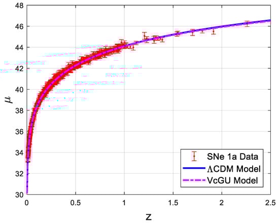
Figure 1.
Supernovae Ia redshift vs. distance modulus data fit with the ΛCDM model and the fit with the new model using the varying speed of light varying gravitational constant , and variable curvature constant (VcGU) model.
It should be mentioned that we are not trying to determine which model fits the SNe 1a data best, as this has already been done in an earlier paper [28] Our attempt is to determine the parameter of the curvature by fitting the data.
We get from the table. Therefore, we may rewrite Equation (29) in the VcGU model as:
in the matter-dominated universe, and in the radiation-dominated universe, as:
If we constrain in th VcGU model (against constraining in the ΛCDM model), we get , and Thus, both the models now have two parameters, with the VcGU model still having a slight edge over the ΛCDM model.
As , both the above expressions, Equations (39) and (40), tend to unity, i.e., the universe was strongly curved in the past. By taking from Table 1 for Equation (39), and from Table 5.2 in reference [7], we get radiation density equal to matter density at , which is determined by the relation:
However, we can easily calculate from Equation (39), and see from Figure 2 displaying the plot of against , that was almost unity within three decimal places at , i.e., well below the redshift when radiation density equaled matter density. The flatness of the universe problem is thus resolved: the universe is curved now and was strongly curved in the past.
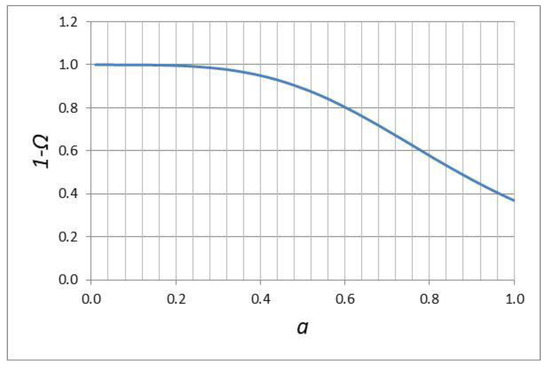
Figure 2.
plotted against using Equation (39).
We can also determine using Equation (26):
This expression shows that must be negative () in order for to be real, i.e., the universe is open with .
We will now determine how the radius of curvature in Equations (3) and (4), which is embedded in the parameter , varies with the scale factor . Now, , and , and . Therefore, This is presented in Figure 3.
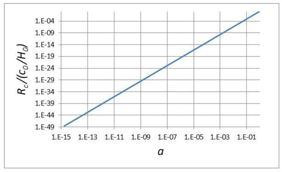
Figure 3.
Curvature in units of plotted against .
Einstein introduced his most undesirable cosmological constant to prevent the universe from collapsing [29]. Currently, it represents the elusive dark energy in most cosmological models that is needed to explain observables. The inflation theories require to be 107 orders of magnitude larger during inflation than in the current epoch. Additionally, it has to be turned on and off at appropriate times: inflation started at and lasted for a period of about [7]. The variable physical constants model, and its extension by relaxing the usual constraint on the curvature of the universe to evolve exactly as the scale factor, makes it possible to refrain from using the cosmological constant in cosmological modeling.
One major objection to the current model is that the Einstein equations represented by Equation (2) are not valid for the varying physical constants, especially the varying speed of light, and thus Equations (3) and (4)—which are derived from it—are incorrect. Nevertheless, if we give Equations (3) and (4) an identity independent of Equation (2), i.e., forget that they are derived from Equation (2), we may then relax the constraint on any of the parameters in Equations (3) and (4), and consider them empirical rather than theoretical. This then poses a challenge to theoreticians to show why these equations fit the observables so well and avoid issues such as the flatness problem. Perhaps the Einstein equations remain valid for variable speed of light except for the space-time regions that are strongly curved due to extremely high energy density such as that in the black holes.
Another concern one would have is that many cosmological observations require for their interpretation the constancy of the speed of light. It is not clear how the observations would modify if is allowed to vary. Nevertheless, we believe the redshift measurements used in this paper, as well as the distance modulus derived from the luminosity measurements, are independent of the speed of light.
7. Conclusions
The following are the conclusions:
- The variable physical constant approach can naturally eliminate the flatness problem that has been pervasive in most cosmological models.
- The universe is open type, was strongly curved in the past, and is substantially curved at present with a curvature .
- The scaling of the curvature can be reliably determined by fitting the most recently available supernovae 1a data; the new model fits the data better than the standard CDM model.
- The radius of curvature of the universe evolves differently than assumed in the standard model; it evolves proportional to the .
- The cosmological constant, and consequently the dark energy, is no longer required to save the cosmos from collapsing.
Funding
This research received no external funding.
Acknowledgments
The author is grateful to Dan Scolnic for providing the SNe Ia Pantheon Sample data used in this work. He expresses his special thanks to the three anonymous reviewers of the paper for their very constructive critical comments which helped to improve the quality of this paper.
Conflicts of Interest
The author declares no conflict of interest.
References
- Penzias, A.A.; Wilson, R.W. A Measurement of Excess Antenna Temperature at 4080 Mc/s. Astrophys. J. 1965, 142, 419–421. [Google Scholar] [CrossRef]
- Guth, A.H. Inflationary universe: A possible solution for the horizon and flatness problem. Phys. Rev. D 1981, 23, 347–356. [Google Scholar] [CrossRef]
- Albrecht, A.; Steinhardt, P.J. Cosmology for Grand Unified Theories with Radiatively Induced Symmetry Breaking. Phys. Rev. Lett. 1982, 48, 1220–1223. [Google Scholar] [CrossRef]
- Linde, A. A new inflationary universe scenario: A possible solution of the horizon, flatness, homogeneity, isotropy and primordial monopole problems. Phys. Lett. B 1982, 108, 389–393. [Google Scholar] [CrossRef]
- Gupta, R.P. Varying physical constants, astrometric anomalies, redshift and Hubble units. Galaxies 2019, 7, 55. [Google Scholar] [CrossRef]
- Olive, K.A. Inflation. Phys. Rep. 1990, 190, 307–403. [Google Scholar] [CrossRef]
- Ryden, B. Introduction to Cosmology; Cambridge University Press: Cambridge, UK, 2017. [Google Scholar]
- Levine, J.; Freese, K. Possible solution to the horizon problem: Modified aging in massive scalar theories of gravity. Phys. Rev. D 1993, 47, 4282–4291. [Google Scholar] [CrossRef] [PubMed]
- Hu, Y.; Turner, M.S.; Weinberg, E.J. Dynamical solutions to the horizon and flatness problems. Phys. Rev. D 1994, 49, 3830–3836. [Google Scholar] [CrossRef]
- Barrow, J.D.; Tipler, F. Analysis of the generic singularity studies by Belinskii, Khalatnikov, and Lifschitz. Phys. Rep. 1979, 56, 371–402. [Google Scholar] [CrossRef]
- Belinski, V.A.; Khalatnikov, I.M.; Lifshitz, E.M. A general solution of the Einstein equations with a time singularity. Adv. Phys. 1982, 31, 639–667. [Google Scholar] [CrossRef]
- Singal, A.K. Horizon, homogeneity and flatness problems – do their resolutions really depend upon inflation? arXiv 2016, arXiv:1603.01539. [Google Scholar]
- Barrow, J.D.; Magueijo, J. Solution to the quasi-flatness and quasi-lambda problems. Phys. Lett. B 1999, 447, 246–250. [Google Scholar] [CrossRef]
- Barrow, J.D.; Magueijo, J. Solving the flatness and quasi-flatness problems in Brans-Dicke cosmologies with varying light speed. Class. Quantum Grav. 1999, 16, 1435–1454. [Google Scholar] [CrossRef]
- Berera, A.; Gleiser, M.; Ramos, R.O. A first principle warm inflation model that solves cosmological horizon and flatness problems. Phys. Rev. Lett. 1999, 83, 264–267. [Google Scholar] [CrossRef]
- Lake, K. The flatness problem and Λ. Phys. Rev. Lett. 2005, 94, 201102. [Google Scholar] [CrossRef] [PubMed]
- Fathi, M.; Jalalzadeh, S.; Moniz, P.V. Classical universe emerging from quantum cosmology without horizon and flatness problems. Eur. Phys. J. C 2016, 76, 527. [Google Scholar] [CrossRef]
- Bramberger, S.F.; Coates, A.; Magueijo, J.; Mukohyama, S.; Namba, R.; Watanabe, Y. Solving the flatness problem with an anisotropic instanton in Horava-Lifshitz gravity. Phys. Rev. D 2018, 97, 043512. [Google Scholar] [CrossRef]
- Narlikar, J.V. An Introduction to Cosmology, 3rd ed.; Cambridge University Press: Cambridge, UK, 2002. [Google Scholar]
- Barrow, J.D. Cosmologies with varying light speed. Phys. Rev. D 1999, 59, 043515. [Google Scholar] [CrossRef]
- Scolnic, D.M.; Jones, D.O.; Rest, A.; Pan, Y.C.; Chornock, R.; Foley, R.J.; Huber, M.E.; Kessler, R.; Narayan, G.; Riess, A.G.; et al. The Complete Light-curve Sample of Spectroscopically Confirmed SNe Ia from Pan-STARRS1 and Cosmological Constraints from the Combined Pantheon Sample. Astrophys. J. 2018, 859, 101. Available online: https://archive.stsci.edu/hlsps/ps1cosmo/scolnic/https://github.com/dscolnic/Pantheon (accessed on 10 May 2019). [CrossRef]
- Peebles, P.J.E. Principles of Physical Cosmology; Princeton University Press: Princeton, NJ, USA, 1993. [Google Scholar]
- Baes, M.; Camps, P.; Van De Putte, D. Analytical expression and numerical evaluation of the luminosity distance in a flat cosmology. Mon. Not. R. Astron. Soc. 2017, 468, 927–930. [Google Scholar] [CrossRef]
- Zaninetti, L. A new analytical solution for the distance modulus in flat cosmology. Int. J. Astron. Astrophys. 2019, 9, 51–62. [Google Scholar] [CrossRef][Green Version]
- Scolnic, D.M.; (University of Chicago). Personal Email communication, 22 November 2018.
- Press, W.H.; Teukolsky, S.A.; Vetterling, W.T.; Flannery, B.P. Numerical Recipes in C—The Art of Scientific Computing, 2nd ed.; Cambridge University Press: Cambridge, UK, 1992. [Google Scholar]
- Walker, J. Chi-Square Calculator. Available online: https://www.fourmilab.ch.rpkp/experim-ents/analysis/chiCalc.html (accessed on 3 August 2019).
- Gupta, R.P. Weighing cosmological models with SNe 1a and gamma ray burst redshift data. Universe 2019, 5, 102. [Google Scholar] [CrossRef]
- Einstein, A. Kosmologische Betrachtungen zur allgemeinen Relativitatstheorie, Sitzungsberichte der Preussischen Akad. d. Wissenschaften 1917, 142–152. [Google Scholar]
© 2019 by the author. Licensee MDPI, Basel, Switzerland. This article is an open access article distributed under the terms and conditions of the Creative Commons Attribution (CC BY) license (http://creativecommons.org/licenses/by/4.0/).