Article

Investigation of Couple Stress Fluid and Surface Roughness Effects in the Elastohydrodynamic Lubrication Problems using Wavelet-Based Decoupled Method

by
Siddu C. Shiralashetti
* and
Mounesha H. Kantli
Department of Mathematics, Karnatak University, Dharwad-580003, India
*
Author to whom correspondence should be addressed.
Lubricants 2016, 4(1), 9; https://doi.org/10.3390/lubricants4010009
Submission received: 13 December 2015 / Revised: 13 February 2016 / Accepted: 11 March 2016 / Published: 21 March 2016

Abstract

:
The standard decoupled method with Newton-generalized minimum residual procedure performs poorly or may break down when used to solve certain elastohydrodynamic lubrication problems. The authors Zargari et al., 2007 presented decoupled and coupled methods in which the limitations of the decoupled method for some set of physical parameters and slight variation in these values (physical parameters) give a non-convergence solution. To overcome this aspect the wavelet-based preconditioners technique is used in this paper to solve the elastohydrodynamic lubrication problem. The effect of coupled stress fluids on elastohydrodynamic lubrication behavior in smooth, as well as rough, contact is investigated using the proposed method, numerically, in a low-speed-high load condition. The elastohydrodynamic lubrication characteristics computed for couple stress fluids are found to have strong dependence on the couple stress parameter, which shows the versatility and applicability of the proposed method.

1. Introduction

The elastohydrodynamic lubrication (EHL) problem is modeled by two main groups of equations, the first concerned with the physical model of the lubricant and the second one governing the lubrication problem, itself. The lubricant model specifies the dependence of the fluid viscosity ( η ) and density ( ρ ) on the pressur ( P ) . These are empirical relations and are highly nonlinear, since most lubricants are non-Newtonian fluids [1,2]. The governing equations consist of the following: the Reynolds equation, the film thickness equation, and the force balance equation. The system of equations is derived from a dimensionless, thin-film approximation of the Stokes equation, coupled with a linear elastic model of the contacting surfaces. The inlet boundary and the free cavitation point boundary define the region where the Reynolds equation is valid. The main objective of the present work is to detect the location of the cavitation point using the proposed wavelet-based decoupled method. Subsequently, the present study addresses the compressible EHL problem involving the effect of couple stress fluid in smooth as well as rough line contacts. The constitutive relationship for couple stress fluids is presented by Stokes [3] in the analysis to derive the modified Reynolds equation in terms of a dimensionless couple stress parameter which represents the molecular length of the additives. The surface roughness is assumed to be single-sided, transverse, and sinusoidal [4,5,6,7].
The ill-conditioned matrices in the system of non-linear algebraic equations arising in EHL confine the application of even more powerful schemes of the Krylov subspace method. The suitable remedy is the preconditioning for such matrices. Classical preconditioners are incomplete LU decomposition (ILU), the approximate inverse preconditioner, etc. [8,9,10]. However, there are large classes of matrices occurring in the modeling of problems which are not amenable to these latest non-stationary iterative schemes with classical preconditioners for their solutions. Zargari et al. [11] used versatile MatLab code from KINSOL in analyzing EHL line contact problems. They observed that the decoupled scheme does not give a convergent solution for some set of physical parameters. Wavelet-based preconditioners provide some remedy in such challenging cases. Chen [12] highlighted the construction and implementation of various wavelet-based preconditioners for the solution of large classes of ill-conditioned systems very effectively. In EHL, an appeal to such schemes has resulted in the construction of suitable wavelet-based preconditioners [13]. The dense and diagonal singular structure of the Jacobian demands more sophisticated iteration schemes from Krylov subspaces. The linear system is A x = b , if A is a symmetric and positive definite then the conjugate gradient (CG) method works well, whereas for non-symmetric and other systems, the generalized minimum residual method (GMRES) can be used [14,15,16]. As the Jacobian matrix is full in EHL problems, the convergence of the iteration is not guaranteed and takes a large number of iterations to converge. It is essential to find effective preconditioners. The Jacobian matrices in EHL are dense with a non-smooth diagonal and smooth away from the diagonal band. This smoothness of the matrix transforms into smallness in the wavelet transform and facilitates in the design or construction of efficient preconditioners using discrete wavelet transform (DWT). DWT with permutation (DWTPer) are designed and implemented by [12,13]. In this paper, we developed the wavelet-based decoupled method for the investigation of surface roughness effects in EHL line contact problems using a couple stress fluid.
This paper is arranged as follows: Section 2 contains the discrete wavelet transform. The wavelet-based decoupled method of the solution is discussed in Section 3. Section 4 presents the method of implementation and numerical findings. In Section 5, results and discussions are given. Finally, the conclusion of the proposed work is discussed in Section 6.

2. Discrete Wavelet Transform (DWT)

A major problem in the growth of wavelets during the 1980s was the search for a multiresolution analysis where the scaling function was compactly supported and continuous. As we already know, the Haar multiresolution analysis is generated by a compactly-supported scaling function, but it is not continuous. The B-splines are continuous and compactly supported but fail to form an orthonormal basis. A family of multiresolution analyses was generated by scaling functions, which are both compactly supported and continuous. These multiresolution analyses were first constructed by Daubechies [17,18], which created great eagerness among mathematicians and scientists conducting research in the area of wavelets.

2.1. Multiresolution Analysis

Wavelets are functions generated from one single function called the mother wavelet by the simple operations of dilation and translation. A mother wavelet gives rise to a decomposition of the Hilbert space L 2 ( R ) , into a direct sum of closed subspaces W j ,    j Z [17].
Let ψ j ,    k ( x ) = 2 j / 2 ψ ( 2 j x k ) and:
W j = c los L 2 ( ) [ ψ j ,    k : k Z ]
Then every f L 2 ( R ) has a unique decomposition:
f ( x ) =    .     .     .     + s 1 + s 0 + s 1 +     .     .     .
where s j W j for all j Z , it is:
L 2 ( R ) = j W j =     .     .     .     W 1 W 0 W 1     .     .     .
Using this decomposition of L 2 ( R ) , a nested sequence of closed subspaces V j ,    j Z of L 2 ( R ) can be obtained, defined by:
V j =     .     .     .     W j 2 W j 1
These closed subspaces { V j ,    j Z } of L 2 ( R ) , form a “multiresolution analysis” with the following properties:
(i)
.      .      .     V 1 V 0 V 1     .      .      .
(ii)
clos L 2 ( V j ) = L 2 ( R )
(iii)
V j = { 0 }
(iv)
V j + 1 = V j W j
(v)
f ( x ) V j f ( 2 x ) V j + 1 ,    j Z
Let ϕ V 0 , the so-called “scaling function” that generates the multiresolution analysis { V j } j Z of L 2 ( R ) . Then:
{ ϕ ( k ) : k Z }
is a basis of V 0 , and by setting:
ϕ j , k ( x ) = 2 j / 2 ϕ ( 2 j x k )
it follows that, for each j Z , the family:
{ ϕ j , k : k Z }
is also a basis of V j .
Then, since ϕ V 0 is in V 1 and since { ϕ 1 , k : k Z } is a basis of V 1 , there exists a unique sequence a k that describes the following “two-scale relation”:
ϕ ( x ) = k = a k ϕ ( 2 x k )
of the scaling function ϕ [19].

2.2. Daubechies’s Wavelets

Different choices for ϕ may yield different multiresolution analyses and the most useful scaling functions are those that have compact support. As an example of multiresolution analysis, a family of orthogonal Daubechies wavelets with compact support has been constructed by Daubechies [18].
A wavelet basis is orthonormal if any two translated or dilated wavelets satisfy the condition:
ψ n , k ( x ) ψ m , l ( x ) d x = δ n , m δ k , l
where δ is the Kronecker Delta function.
Each wavelet family is governed by a set of 2 J (an even integer) coefficients, a k : k =    0 ,    1 ,     .     .     .     ,    2 J 1 through the two-scale relation:
ϕ 2 J ( x ) = k = 0 2 J 1 a k ϕ 2 J ( 2 x k )
Based on the scaling function ϕ 2 J ( x ) , the mother wavelet can be written as:
ψ 2 J ( x ) = k = 2 2 J 1 b k ϕ 2 J ( 2 x k )
Since the wavelets are orthonormal to the scaling basis, the coefficients of the scaling function and the mother wavelet for the two-scale equation are related by:
b k = ( 1 ) k a 2 J 1 k
Daubechies [17] found and exploited the link between vanishing moments of the wavelet ψ and regularity of the wavelet and scaling functions, ψ and ϕ . The wavelet function ψ has K vanishing moments if:
x k ψ ( x ) d x = 0 for 0 k K
and a necessary and sufficient condition for this to hold is that the integer translates of the scaling function ϕ exactly interpolate polynomials of degree up to K. That is, for each k, there exists constants c l such that:
x k = l c l k ϕ l ( x )
Daubechies introduced scaling functions satisfying this property and distinguished by having the shortest possible support. The scaling function ϕ 2 J has suppor [ 0 ,    2 J 1 ] , while the corresponding wavelet function ψ 2 J has support in the interval [ 1 2 J / 2 ,    2 J / 2 ] and has ( 2 J / 2 1 ) vanishing wavelet moments. Thus, according to Equation (8) Daubechies scaling functions of order 2 J can exactly represent any polynomial of order up to, but not greater than 2 J / 2 1 [18]. For example, Daubechies family of wavelets when N = 4 , we have low-pass filter coefficients [19], h 0 = 1 + 3 4 2 , h 1 = 3 + 3 4 2 , h 2 = 3 3 4 2 , and h 3 = 1 3 4 2 , and g 0 = 1 3 4 2 , g 1 = 3 3 4 2 , g 2 = 3 + 3 4 2 , and g 3 = 1 + 3 4 2 are the high-pass filter coefficients.

2.3. Discrete Wavelet Transform Matrix

A DWT matrix is a linear transformation that transforms vectors from the standard basis to a wavelet basis. Certain classes of linear operators that correspond to dense matrices in the standard basis can be approximated by sparse matrices in a suitably-chosen wavelet basis. We use this property to design preconditioners for linear systems based on representing the system in a wavelet basis and forming a sparse approximation to the transformed matrix [20]. The process of applying a DWT matrix to a dense matrix in order to obtain a sparse approximation is known as wavelet compression. The DWT of a n     ×     n matrix, we form the orthogonal matrices ( W 1 , W 2 ,    .    .    .    ,    W k ) are as follows:
W 1 = [ h 0     h 1     h 2     h 3     0      0       .      .       .        0 0      0      h 0     h 1     h 2     h 3    0      .     .     .     0 .                                                                 . .                                                                 . .                                                                 . h 2      h 3     0        .       .       .       0       h 0       h 1 g 0      g 1    g 2      g 3      0       0     .      .      .     0 0        0     g 0      g 1      g 2     g 3    0    .    .    .    0 .                                                                . .                                                                . .                                                                . g 2      g 3     0        .       .       .       0      g 0      g 1 ] n × n , W 2 = [ h 0     h 1     h 2     h 3     0      0      .      .      .       0 0      0      h 0     h 1      h 2    h 3    0     .     .     .     0 .                                                                 . .                                                                 . .                                                                 . h 2     h 3     0      0    .       .       .       0      h 0      h 1 g 0     g 1    g 2    g 3      0       0      .      .       .     0 0        0      g 0    g 1     g 2     g 3    0    .     .     .    0 .                                                                . .                                                                . .                                                                . g 2      g 3     0        .       .       .       0      g 0     g 1 ] n 2 × n 2 , , W k = [ h 2     h 3 g 2    g 3 ] 2 × 2

2.4. Discrete Wavelet Transform with Permutation (DWTPer) Matrix

The standard DWT is not adapted to compressing matrices with non-smooth (NS) diagonal bands for preconditioning purposes because the pattern of non-zero elements in the compressed matrix tends to lead to a large amount of fill-in during LU factorization. One way of avoiding this problem is to use NS-forms, which we consider briefly here. We then present the non-standard DWT with permutation (DWTPer) and look in detail at its effect on dense matrices with non-smooth features both on and off the diagonal. Ford [21] proposed the DWTPer as an alternative way of avoiding the creation of finger pattern matrices. This is implemented by performing a standard DWT followed by a permutation of the rows and columns of the matrix to center the fingers about the leading diagonal. The DWTPer matrices ( W 1 , W 2 ,    .    .    .    , W k ) are as follows:
W 1 = [ h 0      Φ      h 1     Φ     h 2     Φ     h 3     Φ     .      .      .     Φ Φ       I      Φ      Φ      Φ     Φ      Φ      Φ     .      .       .     Φ g 0     Φ      g 1     Φ      g 2    Φ      g 3    Φ     .      .       .     Φ Φ      Φ      Φ      I       Φ     Φ      Φ      Φ     .      .       .     Φ .                                                                               . .                                                                               . .                                                                               . h 2     Φ     h 3     Φ      .     .      .      Φ      h 0     Φ     h 1     Φ Φ     Φ      Φ      Φ      .      .      .       Φ      Φ      I     Φ     Φ g 2    Φ      g 3     Φ      .      .      .       Φ      g 0    Φ     g 1    Φ Φ     Φ      Φ      Φ      .      .      .       Φ      Φ      Φ     Φ      I ] n × n , W 2 = [ h 0     Φ     h 1     Φ     h 2     Φ     h 3     Φ     .      .      .     Φ Φ      I      Φ     Φ      Φ      Φ     Φ      Φ     .      .       .     Φ g 0    Φ      g 1    Φ      g 2     Φ     g 3     Φ     .      .       .     Φ Φ     Φ      Φ      I      Φ      Φ     Φ      Φ     .      .       .     Φ .                                                                               . .                                                                               . .                                                                               . h 2     Φ     h 3     Φ     .      .      .      Φ      h 0     Φ     h 1     Φ Φ     Φ      Φ      Φ      .      .      .      Φ      Φ      I     Φ      Φ g 2    Φ      g 3     Φ      .      .      .      Φ      g 0     Φ     g 1    Φ Φ     Φ      Φ      Φ      .      .      .      Φ      Φ      Φ     Φ      I ] n 2 × n 2 , , W k = [ h 3      0 0         1 ] 2 × 2
Here, each I is an identity matrix of dimension 2 J 1 1 and the Φ ’s are block zero matrices of the appropriate sizes. For J = 1, both I and Φ are of dimension 0.

3. Wavelet-Based Decoupled Method for the Numerical Solution of EHL Problem

The multigrid method is commonly used to solve the Reynolds equation efficiently [22,23]. Since EHL problems are nonlinear, the wavelet-based decoupled method is appropriate. (i) We begin with an initial guess for P, H 0 , and the cavitation point X c ; (ii) evaluate H from the film thickness equation; (iii) solve the Reynolds equation for P; (iv) update H 0 using the force balance equation; (v) move the cavitation point based upon the value of d P d X at the cavitation point; (vi) while not converged, go to (ii); (vii) the overall method is such that the cavitation point is only updated on the finest grid and H 0 is only updated on the coarsest level so as to ensure smooth convergence of the whole method; and (viii) numerical under-relaxation parameters C 1 and C 2 are used for pressure and film thickness equations, respectively, at (iii) and (iv).
A detailed method of solution of the proposed method is as follows.
To initiate the wavelet-based decoupled method for the solution of EHL problem with line contacts using couple stress fluid and surface roughness effects, an initial guess is made for pressure ( P ) distribution and the offset film thickness H 0 [24]. These values use the calculation of film thicknes ( H ) , density ( ρ ) [25], and viscosity ( η ) [26], respectively. The Reynolds equation is discretized over a uniform mesh of different mesh sizes using finite difference approximation and solved along with the film thickness equation and force balance equation using the wavelet-based decoupled method as follows,
Consider the Reynolds equation of the form:
d 2 P d X 2 = F ( X ,     P ,      d P d X , H , η , ρ , X c )
with:
P ( X i n ) = P ( X o u t ) = d P ( X c ) d X = 0
Taking the initial values of Hertzian pressure P ( x ) = { 1 x 2     i f     | x | < 1        0           otherwise , X c = 0 and H 0 = 1 4 1 2 log 2 [24], then evaluates H from the film thickness equation.
Finite difference discretization of Equation (15) gives the system of nonlinear algebraic equations:
F j ( P 1 ,    P 2 ,    .    .    .    ,    P n , H 1 , H 2 , ...... H n ) = 0 ,      1 j n
where n = 2 J , n is the number of grid points and J is the level of resolution.
The nonlinear systems of Equation (17) can be solved using Newton’s method as follows:
P n + 1 = P n C 1 F ( P n ) F ( P n ) P n + 1 = P n C 1 S n
where C 1 = 0.4    ( 0 < C 1 < 1 ) is the under-relaxation parameter:
Let,
S n = F ( P n ) F ( P n )
Equation (19) reduces to the linear system of equations:
B x = f
where B = [ F ( P n ) ] n × n ,    x = [ S n ] n × 1 , f = [ F ( P n ) ] n × 1 .
Applying the DWT-based decoupled method (DWT-DM) or DWTPer-based decoupled method (DWTPer-DM) up to Jth level to Equation (20) as follows:
First level: Equation (20) reduced to:
[ W 1 ] n    ×    n [ B ] n    ×    n [ W 1 T ] n    ×    n     [ x ] n    ×    1 = [ W 1 ] n    ×    n [ f ] n    ×    1 B 1 x 1 = f 1
Second level: Equation (21) becomes:
[ [ W 2 ] n 2 × n 2     [ Φ ] n 2 × n 2 [ Φ ] n 2 × n 2        [ I ] n 2 × n 2 ] n    × n [ B 1 ] n    × n [ [ W 2 T ] n 2 × n 2     [ Φ ] n 2 × n 2 [ Φ ] n 2 × n 2           [ I ] n 2 × n 2 ] n    × n     [ x 1 ] n    × 1 = [ [ W 2 ] n 2 × n 2     [ Φ ] n 2 × n 2 [ Φ ] n 2 × n 2       [ I ] n 2 × n 2 ] n    ×    n [ f 1 ] n    × 1 B 2 x 2 = f 2
Jth level: At the coarsest level we have:
[ [ W J ] 2 × 2     [ Φ ] 2 × n 2 [ Φ ] n 2 × 2 [ I ] n 2 × n 2 ] n × n [ B J 1 ] n × n [ [ W J T ] 2 × 2     [ Φ ] 2 × n 2 [ Φ ] n 2 × 2 [ I ] n 2 × n 2 ] n × n [ x J 1 ] n × 1 = [ [ W J ] 2 × 2     [ Φ ] 2 × n 2 [ Φ ] n 2 × 2 [ I ] n 2 × n 2 ] n × n [ f J 1 ] n × 1 B J x J = f J
Consider the transformed linear system at the Jth level (coarsest level) in Equation (23), from which we can write B J as B J = D J + C J [7] based on operator (matrix) splitting. Then, we need to choose an efficient preconditioner matrix M = D J . Multiplying M 1 on both sides of Equation (23), we get:
M 1 B J    x J    =    M 1 f J
Solving Equation (24) iteratively, we obtain x J . Now applying successively the inverse discrete wavelet transform-based decoupled method (IDWT-DM) or the inverse discrete wavelet transform with permutation-based decoupled method (IDWTPer-DM) to x J at the level J, which reduces to x J 1 = [ [ W J T ] 2 × 2    [ Φ ] 2 × n 2 [ Φ ] n 2 × 2       [ I ] n 2 × n 2 ] n × n [ x J ] n × 1 . Again, applying IDWT-DM or IDWTPer-DM to x J 1 , at the level J − 1, we get x J 2 = [ [ W J 1 T ] 4 × 4     [ Φ ] 4 × n 4 [ Φ ] n 4 × 4      [ I ] n 4 × n 4 ] n × n [ x J 1 ] n × 1 , and so on up to finer levels, IDWT-DM or IDWTPer-DM to x 1 , which finally gives x = [ W 1 T ] n × n [ x 1 ] n × 1 .
Substitute x    ( = S n ) in Equation (18) we get the required pressure P.
Fix the cavitation point X c using d P d X = 0   at  X = X c , which we can write as P i P i + 1 Δ x = 0    at   X = X c . If the pressure gradient is zero at the initial guess X c is fine. Otherwise, move X c one interval to the left or right depending on whether ( P i P i + 1 Δ x ) X c > 0 or ( P i P i + 1 Δ x ) X c < 0 , respectively. Approximate a new cavitation point X c and solve the EHL problem. If the pressure gradient is zero at X c then we get a converged solution; otherwise check for the condition whether:
( P i P i + 1 Δ x ) X c × ( P i P i + 1 Δ x ) X c < Tol ( = 1 E - 06 )
We obtain the residual (Res) from the following force balance Equation (26):
Res = Δ x j = 0 n 1 ( P j + P j + 1 2 ) π 2 = 0
and then update H 0 in the following Equation (26):
H 0 = H 0 + Res  C 2
where C 2 = 0.03    ( 0 < C 2 < 1 ) is the under-relaxation parameter for pressure.
If condition Equation (25) is not met, repeat the procedure.

4. Numerical Experiment

Consider the governing modified Reynolds equation [4,27] in its dimensionless form:
X ( ρ ¯ H 3 η ¯ ξ P X ) k X ( ρ ¯ H ) = 0
where, k = 3 U π 2 4 W 2 , ξ = [ 1 12 Ω 2 + 24 Ω 3 tanh ( Ω 2 ) ] 1 and Ω = 8 W H π  Lm with the boundary conditions, inlet boundary P = 0 at X = X i n , and outlet boundary P = P X = 0 at X = X o u t . The film thickness equation incorporating the sinusoidal roughness term in dimensionless form is given as:
H ( X ) = H 0 + X 2 2 + ν ¯ + A sin ( 2 π X λ )
where ν ¯ = ν R b 2 is the dimensionless surface displacement given by:
ν ¯ = 1 2 π X i n X o u t P log ( X S ) 2 d S
The dimensionless force balance equation is given by:
X i n X o u t P d X = π 2
The dimensionless form of viscosity η ¯ ( P ) [25] and density ρ ¯ ( P ) [26], are given by:
η ¯ = exp [ ( log η 0 + 9.67 ) × { 1 + ( 1 + 5.1 E - 09 P p h ) z } ]
and:
ρ ¯ = ( 1 + 0.6 E - 09 P p h 1 + 1.7 E - 09 P p h )
where z = 0.6 , η 0 = 1.98 E + 08 and p h = 1.84 E + 09 . The three non-dimensional physical parameters that characterize the line contact problem are velocity (U), load force (W), and elasticity (G) [11]. The spatial domain X [ X i n , X o u t ] is discretized with a uniform grid of n points X i ( 1 i n ) . Consider the cavitation point X c to be located at an unknown internal poin X j ( 2 j n 1 ) . The Equations (28), (29), and (31) are discretized using second-order finite differences with uniform grid points x i ,    1 i n , and the domain of interest is [ X i n , X o u t ] = [ 2 , 1.5 ] , X c is the cavitation point to be determined in the solution process. The discretized form of modified Reynolds equation [27]:
( ε i + ε i + 1 2 ) ( P i + 1 P i Δ x ) ( ε i + ε i 1 2 ) ( P i P i 1 Δ x ) Δ x k ( ρ i H i ρ i 1 H i 1 Δ x ) = 0
where ε i = ρ ¯ i H i 3 η i ξ .
The film thickness equation approximated at x i on the regular grid is given by:
H ( x i ) = H 0 + x i 2 2 1 2 π j = 1 n K i j P ( x j ) + A sin ( 2 π x j λ )
where:
K i j = ( x i x j + Δ x 2 ) ( log | x i x j + Δ x 2 | 1 ) ( x i x j Δ x 2 ) ( log | x i x j Δ x 2 | 1 )
for i = 0 , 1 , 2 ,    .    .    .    , n and j = 0 , 1 , 2 ,    .    .    .    , n , and the force balance equation in discrete from is:
Δ x j = 0 n 1 ( P j + P j + 1 2 ) π 2 = 0
Use boundary conditions in Equations (34), (35), and (37) by taking the initial values of P , X c , and H 0 , then solving Equation (35), we get H. Next, we take Equation (34) in the form of F ( P i ) = 0 to solve this system using procedure explained in Section 3. The numerical results are presented in figures and tables, which are shown in next section.

5. Results and Discussion

The EHL characteristics are presented for one set of physical parameters, i.e., low speed-high load ( U = 2 E - 11 ,    W = 4 E - 04 ) , maximum Hertzian pressure ( p h = 5.8 E + 08 ) . The results are obtained using the values of input parameters given in Table 1. The method in [11] is not converged for some set of physical parameters, whereas the proposed method overcomes the above limitations, which shown in Table 2 and Figure 1, Figure 2 and Figure 3 for different grid points. Figure 4a,b presents the numerical solutions of pressure profile and film shapes respectively, using wavelet-based decoupled method for pure base oil ( Lm = 0 ) with three values of couple stress parameter Lm = 1 E - 05 ,    2 E - 05 ,    5 E - 05 for a low speed-high load ( U = 2 E - 11 ,    W = 4 E - 04 ) condition. It is clear from Figure 4a,b that, couple stress fluids cause negligible change in the pressure profile and film thickness, respectively. Figure 5a,b represents the detailed solution presented in Figure 4a,b. On closer examination, it is observed that pressure increases marginally with an increase in Lm from 0 to 1 E - 05 , whereas a marginal decrease in pressure as Lm is increased further to 5 E - 05 . Therefore, it implies that the initial rise in pressure due to increased lubricant viscosity is compensated by the pressure reduction caused by fluid film thickening. Figure 6a,b compares the pressure and film thickness solutions, respectively, for the case of rough surface ( A = 0.2 ,    λ = 0.12 ) obtained using pure base oil ( Lm = 0 ) with couple stress fluid at Lm = 1 E - 05 ,    2 E - 05 and 5 E - 05 for low speed-high load ( U = 2 E - 11 ,    W = 4 E - 04 ) condition. It can be seen from Figure 6a that the local pressure peaks at asperity tips for the case of couple stress fluids are marginally lower than those for Newtonian fluid. This is attributed to a reduction in the flow resistance offered by surface roughness due to fluid film thickening, as apparent from Figure 6b, in the case of couple stress fluids. Similarly, Figure 7a,b shows the detailed observations presented in Figure 6a,b.

6. Conclusions

The new decoupled method presented in this paper, called the wavelet-based decoupled method has been shown to be effective and versatile. The standard and other decoupled methods fail to converge for EHL problems discussed in [11]. The wavelet-based decoupled method does ensure such convergence. The properties of wavelets should permit the wavelet-based decoupled method to be efficiently applied in many cases through use of compression. The results shown in this paper have demonstrated that, it is worthwhile to further explore the usefulness of this new decoupled method. The pressure distribution solution varies only marginally when couple stress fluid is employed instead of a Newtonian fluid at low speed-high load. The maximum value of the couple stress parameter used in the analysis. Additionally, the reduction in minimum film thickness due to surface roughness may be compensated by film thickening caused by couple stress fluid and the desired film thickness is obtained by selecting an appropriate value of the couple stress parameter.

Acknowledgments

We are thankful to the anonymous reviewers for their valuable suggestions.

Author Contributions

Siddu C. Shiralashetti: Defining the model of the problem and writing the paper. Mounesha H. Kantli: Implementing the defined problem and writing the paper.

Conflicts of Interest

The authors declare no conflict of interest.

Nomenclature

b half width of the Hertzian contact, b = 8 w R / π E
R reduced radius of curvature,
E reduced modulus of elasticity,
U dimensionless speed parameter, U = ( η 0 u s ) / ( 2 E R )
u velocity component
u s sum velocity, u s = u 1 + u 2
W non-dimensional load parameter, w / ( E R )
w external load per unit width
G dimensionless materials parameter, α E
z pressure viscosity parameter
η Newtonian viscosity
η 0 viscosity at ambient pressure
η ¯ dimensionless viscosity, η / η 0
X c dimensionless location of pressure spike
n number of nodes on grid
Lm Couple stress parameter
ρ Density
ρ 0 density at ambient pressure
ρ ¯ dimensionless density, ρ / ρ 0
H dimensionless film thickness, h R / b 2
h film thickness
h ¯ dimensionless film thickness, h / R ( 2 U ) 1 / 2
H 0 dimensionless constant
K i j discrete approximation of K -logarithmic kernel
P dimensionless pressure, p / P h
p Pressure
p h maximum Hertzian pressure, p h = ( 2 w ) / ( π b )
Δ x mesh size
X dimensionless coordinate x / b , x coordinate
A dimensionless amplitude
λ dimensionless wavelength

References

  1. Dowson, D.; Higginson, G.R. Elasto-Hydrodynamic Lubrication: The Fundamentals of Roller and Gear Lubrication; Pergaman Press: Oxford, UK, 1966. [Google Scholar]
  2. Rao, P.S.; Agarwal, S. Effect of surface roughness on the hydrodynamic lubrication of porous inclined slider bearing considering slip velocity and squeeze velocity with couple stress fluids. Int. J. Eng. Sci. Technol. 2014, 6, 45–64. [Google Scholar] [CrossRef]
  3. Stokes, V.K. Couple stresses in fluids. Phys. Fluids 1966, 9, 1709–1715. [Google Scholar] [CrossRef]
  4. Keshavan, S.; Santhana, K.N. Surface roughnss effects on squeeze film behaviour in porous transversely triangular plates with couple stress fluid. Int. J. Mech. Eng. Technol. 2012, 3, 1–12. [Google Scholar]
  5. Li-Ming, C.; Jaw-Ren, L.; Hsiang-Chen, H.; Yuh-Ping, C. Effects of surface roughness and flow rheology on the EHL of circular contacts with power-law fluid. J. Marine Sci. Technol. 2013, 21, 175–181. [Google Scholar]
  6. Lin, J.R.; Chu, L.M.; Liang, L.J. Effects of viscosity pressure dependency on the non-Newtonian squeeze film of parallel circular plate. Lubr. Sci. 2013, 25, 1–9. [Google Scholar] [CrossRef]
  7. Naduvinamani, N.B.; Apparao, S.; Hiremath, A.G. Effect of Surface Roughness and Viscosity-Pressure Dependency on the Couple Stress Squeeze Film Characteristics of Parallel Circular Plates. Adv. Tribol. 2014. [Google Scholar] [CrossRef]
  8. Bujurke, N.M.; Salimath, C.S.; Kudenatti, R.B.; Shiralashetti, S.C. A fast wavelet-multigrid method to solve elliptic partial differential equations. Appl. Math. Comp. 2007, 185, 667–680. [Google Scholar] [CrossRef]
  9. Bujurke, N.M.; Salimath, C.S.; Kudenatti, R.B.; Shiralashetti, S.C. Wavelet-multigrid analysis of squeeze film characteristics of poroelastic bearings. J. Comp. Appl. Math. 2007, 203, 237–248. [Google Scholar] [CrossRef]
  10. Bujurke, N.M.; Salimath, C.S.; Kudenatti, R.B.; Shiralashetti, S.C. Analysis of modified Reynolds equation using the wavelet-multigrid scheme. Num. Methods Part. Differ. Eqn. 2006, 23, 692–705. [Google Scholar] [CrossRef]
  11. Zargari, E.A.; Jimack, P.K.; Walkley, M.A. An investigation of the film thickness calculation for elastohydrodynamic lubrication problems. Int. J. Numer. Math. Fluids 2007, 1–6. [Google Scholar]
  12. Chen, K. Matrix Preconditioning Techniques and Applications; Cambridge University Press: Cambridge, UK, 2005. [Google Scholar]
  13. Ford, J.M. Wavelet-Based Preconditioning of Dense Linear Systems. Ph.D. Thesis, University of Liverpool, Liverpool, UK, 2001. [Google Scholar]
  14. Saad, Y. Iterative Methods for Sparse Linear Systems; PWS Publishing Company: Boston, MA, USA, 1996. [Google Scholar]
  15. Saad, Y.; Schultz, M.H. GMRES: A generalized minimal residual algorithm for solving non-symetric linear systems. SIAM J. Sci. Stat. Comput. 1986, 7, 856–869. [Google Scholar] [CrossRef]
  16. Kelley, C.T. Iterative Methods for Linear and Nonlinear Equations; SIAM: Philadelphia, PA, USA, 1995. [Google Scholar]
  17. Daubechies, I. Ten Lectures on Wavelets; SIAM: Philadelphia, PA, USA, 1992. [Google Scholar]
  18. Daubechies, I. Orthonormal bases of compactly supported wavelets. Commun. Pure Appl. Math. 1988, 41, 909–996. [Google Scholar] [CrossRef]
  19. Lilliam, A.D.; Maria, T.M.; Victoria, V. Daubechies wavelet beam and plate finite elements. Finite Elements Anal. Design 2009, 45, 200–209. [Google Scholar]
  20. Chen, K. Discrete wavelet transforms accelerated sparse preconditioners for dense boundary element systems. Elec. Trans. Numer. Anal. 1999, 8, 138–153. [Google Scholar]
  21. Ford, J.M. An improved discrete wavelet transeforms based preconditioner for dense matrix problems. SIAM J. Matrix Anal. Appl. 2003, 25, 642–661. [Google Scholar] [CrossRef]
  22. Venner, C.H.; Lubrecht, A.A. Multilevel methods in Lubrication; Elsevier: New York, NY, USA, 2000. [Google Scholar]
  23. Brigges, W.L. A Multigrid Tutorial, 2nd ed.; SIAM: Philadelphia, PA, USA, 2000. [Google Scholar]
  24. Venner, C.H. Multilevel Solution of the EHL Line and Point Contact Problems. Ph.D. Thesis, University of Twente, Byrness Hurd, The Netherlands, 1991. [Google Scholar]
  25. Dowson, D.; Whitaker, A.V. A numerical procedure for the solution of the elastohydrodynamic lubrication problem of rolling and sliding contacts lubricated by a Newtonian fluid. Proc. Inst. Mech. Eng. 1965, 180, 57–71. [Google Scholar]
  26. Roelands, C.J.A.; Vluger, J.C.; Waterman, H.I. The viscosity-temperature-pressure relationship for lubricating oils and its correlation with the chemical construction. ASME J. Basic Eng. 1963, 85, 601–610. [Google Scholar] [CrossRef]
  27. Saini, P.K.; Kumar, P.; Tandon, P. Surface roughness effects in elastohydrodynamic lubrication line contacts using couple stress fluid. Technical Note Proc. IMechE. Part J J. Eng. Trib. 2008, 222, 151–155. [Google Scholar] [CrossRef]
Figure 1. Convergence of the EHL problem using different schemes with couple stress (Lm=1E−05) and surface roughness parameters ( A = 0.2 ,    λ = 0.12 ,     n = 64 ,    U = 2 E - 11 and W = 4 E - 05 ) .
Lubricants 04 00009 g001
Figure 2. Convergence of the EHL problem using different schemes with couple stress (Lm=1E−05) and surface roughness parameters ( A = 0.2 ,    λ = 0.12 ,     n = 128 ,    U = 2 E - 11 and W = 4 E - 05 ) .
Lubricants 04 00009 g002
Figure 3. Convergence of the EHL problem using different schemes with couple stress (Lm=1E−05) and surface roughness parameters ( A = 0.2 ,    λ = 0.12 ,     n = 256 ,    U = 2 E - 11 and W = 4 E - 05 ) .
Lubricants 04 00009 g003
Figure 4. Numerical solution of the EHL problem with couple stress using wavelet-based decoupled method (DWTPer-DM) ( n = 256 ,    U = 2 E - 11 , W = 4 E - 05   and   G = 5 E + 03 ) . (a) Pressure solution; and (b) film thickness solution.
Lubricants 04 00009 g004
Figure 5. Detailed numerical solution of the EHL problem with couple stress around the Petrusevich spike using wavelet-based decoupled method ( n = 256 ,    U = 2 E - 11 , W = 4 E - 05   and   G = 5 E + 03 ) . (a) Pressure solution; and (b) film thickness solution.
Lubricants 04 00009 g005
Figure 6. Numerical solution of the EHL problem using wavelet based decoupled method (DWTPer-DM) with couple stress and surface roughness parameters ( n = 256 ,    U = 2 E - 11 , W = 4 E - 05   and   G = 5 E + 03 ) . (a) Pressure solution; and (b) film thickness solution.
Lubricants 04 00009 g006
Figure 7. Detailed numerical solution of the EHL problem with couple stress and surface roughness around the Petrusevich spike using wavelet based decoupled method ( n = 256 ,    U = 2 E - 11 , W = 4 E - 05   and   G = 5 E + 03 ) . (a) Pressure solution; and (b) film thickness solution.
Lubricants 04 00009 g007
Table 1. Input parameters for EHL analysis.
ParameterValue
Pressure viscosity coefficient, α2.16E−8 P a 1
Equivalent radius of the disks, R0.02 m
Equivalent elastic modulus, E 2.2E+11 Pa
Inlet viscosity, η 0 1.98E+8 P a 1
Table 2. The sensitivity of convergence of three schemes to the physical parameters with couple stress ( Lm = 1 E - 05 ) and surface roughness effects ( A = 0.2 ,    λ = 0.12 ) .
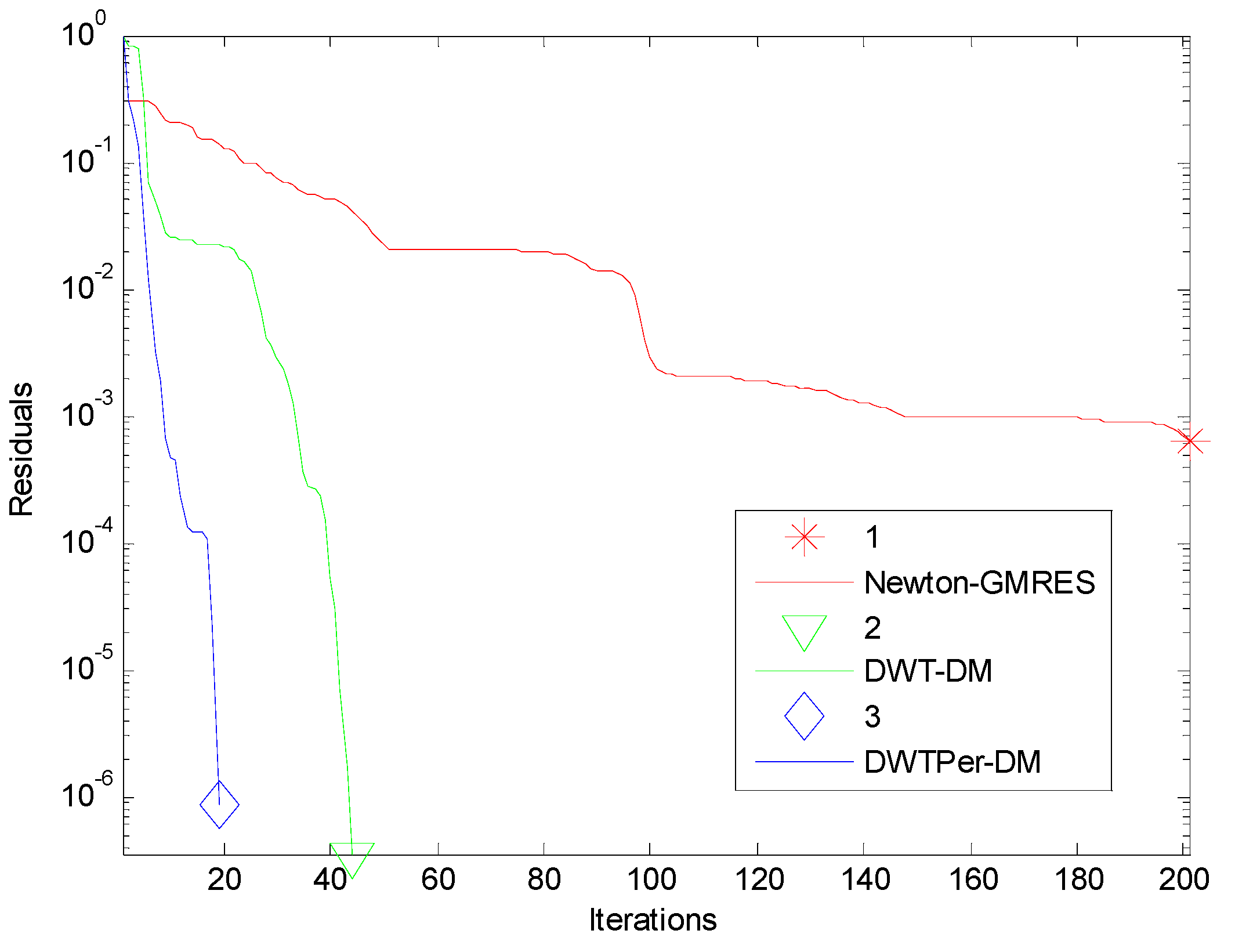
Converged to the Desired Accuracy (Tol=−1E−6)? (Number of Iterations)
n U W G Newton-GMRES [11]DWT-DMDWTPer-DM
2E−114E−55E+3Yes (201)Yes (41)Yes (18)
642E−104E−55E+3NoYes (43)Yes (19)
2E−114E−45E+3Yes (201)Yes (44)Yes (19)
2E−114E−55E+3NoYes (134)Yes (30)
1282E−104E−55E+3NoYes (145)Yes (32)
2E−114E−45E+3NoYes (147)Yes (35)
2E−114E−55E+3NoYes (100)Yes (39)
2562E−104E−55E+3NoYes (108)Yes (41)
2E−114E−45E+3NoYes (109)Yes (45)

