1. Introduction
The flow of thin lubricant films in journal and thrust bearings is most often described by the Reynolds equation of lubrication coupled with the energy transport equation. The numerical solution of these two coupled equations is a problem that has been solved for many decades [
1]. However, it requires a computational effort that can render transient analyses very time consuming. Therefore, efficient solvers and adequate coupling strategies are of major importance to perform complex analyses in a reasonable amount of time.
If film rupture and reformation (traditionally designated as “cavitation”) are absent, and if the flow regime is laminar and isothermal, then the Reynolds equation is an elliptic linear differential equation. A direct solver can be used after its discretization in the thin film plane.
The energy equation contains convective transport terms, conductive transport terms across the thin film, and dissipative source terms arising from its coupling with the Reynolds equation. Its character is therefore not entirely elliptic, and its solver is different from the one used for the Reynolds equation. Moreover, the energy equation must also be discretized across the thin fluid film, and the number of discretization points in this direction must be large enough to capture temperature gradients near the walls. Therefore, the energy equation requires a substantially higher computational effort compared to the Reynolds equation. Developing an accurate and efficient solver for the energy equation is then an important step toward solving non-isothermal lubrication problems. The task is not simple because there is no analytical solution of the complete energy equation to be used for validations. For example, if the analytical solution of the laminar and isothermal thin film flow in a one dimensional (1D) slider can be used to validate the solver of the Reynolds equation, no similar solution exists for the energy equation. For validation, a numerical solver for the energy equation will have to be tested with different wall boundary conditions, and the numerical results must be checked for various grid densities. Such results are absent from the literature.
As mentioned above, the energy equation must also be discretized over the film thickness. The normal practice is to increase the number of discretization cells across the thin film until a grid independent numerical solution is reached, and this renders its solution time consuming. In the natural discretization methods (NDMs), such as the finite difference or finite volumes methods, the variation of the temperature between two cells is linear. This leads to a significant number of discretization cells across the thin film. An efficient approach for solving the energy equation was introduced by Elrod and uses the Legendre polynomials to describe the temperature variation across the thin film [
2]. The coefficients of the Legendre polynomials expansion were first calculated by using a Galerkin approach. Later, Elrod used the collocation method at the Lobatto points; that is, the roots of the derivative of the highest order of the used Legendre polynomial. This method, known as the “Lobatto Points Collocation Method (LPCM)”, proved to be more efficient [
3].
Despite its efficiency, the method is barely used, likely because of its complexity. Thus, Moraru [
4] extended the LPCM to compressible films by describing the variation of the density across the thin film with Legendre polynomials. Feng and Kaneko [
5] used the LPCM to solve the energy equation in aerodynamic foil bearings. Lehne et al. [
6] presented a comprehensive review of the numerical solution strategies of the coupled Reynolds and energy equations, including the LPCM. Except for the cited references, the literature is scarce in references dealing with the LPCM.
This work presents a systematic comparison between the natural discretization method (NDM) of the energy equation and its LPCM approximation. In order to decouple the Reynolds and energy equation, the viscosity is supposed to be constant and the flow laminar. A one dimensional (1D) inclined slider is used for the numerical tests. The Reynolds equation then has an analytical solution, and the analysis is entirely focused on the energy equation. The results for the 1D slider compare both the number of points and the computational time required by the NDM and by the LPCM to obtain grid independent solutions. The results show how the NDM is excessively time consuming when high accuracy is sought, and the net economy of computational time brought by the LPCM approach.
A thermo-hydrodynamic analysis of the 1D slider with the coupled Reynolds and energy equation is then performed. The analysis highlights the same conclusions, namely the large superiority of the LPCM compared to NDM in terms of computational effort. Lastly, a two-lobe journal bearing with axial supply grooves is analyzed to demonstrate the accuracy that can be expected with simple, non-triggered boundary conditions for the energy equation.
2. The Numerical Solution of the Energy Equation Based on the Natural Discretization Method
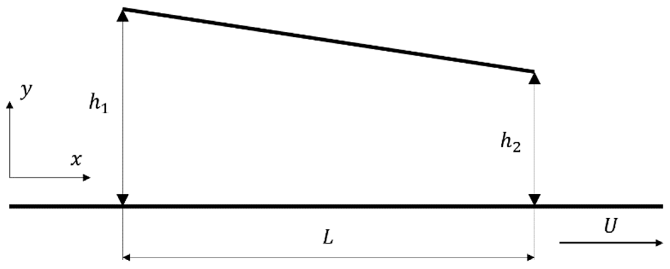
The 1D inclined slider shown in
Figure 1 is used in References [
2,
3] for the resolution of the Reynolds equation coupled with the energy equation. The current work is focused on the resolution of the energy equation decoupled from the Reynolds equation, for which an analytical solution is used. This gives an accurate numerical solution of the energy equation without the influence of the coupling with pressure and velocities affected by numerical uncertainties. The numerical data used is detailed in
Table 1.
The conservative form of the energy equation for the lubrication thin film flow of an incompressible fluid writes [
1]:
It contains the convection transport terms on its left hand side, and the temperature diffusion and dissipation terms on its right hand side. The terms on the right hand side are simplified according to the lubrication thin film assumption; that is, only derivatives across the thin film are taken into account.
The dimensionless coordinate
is introduced to take into account that the film thickness
is not constant.
Following this coordinate transformation, the energy Equation (1) for the 1D slider becomes:
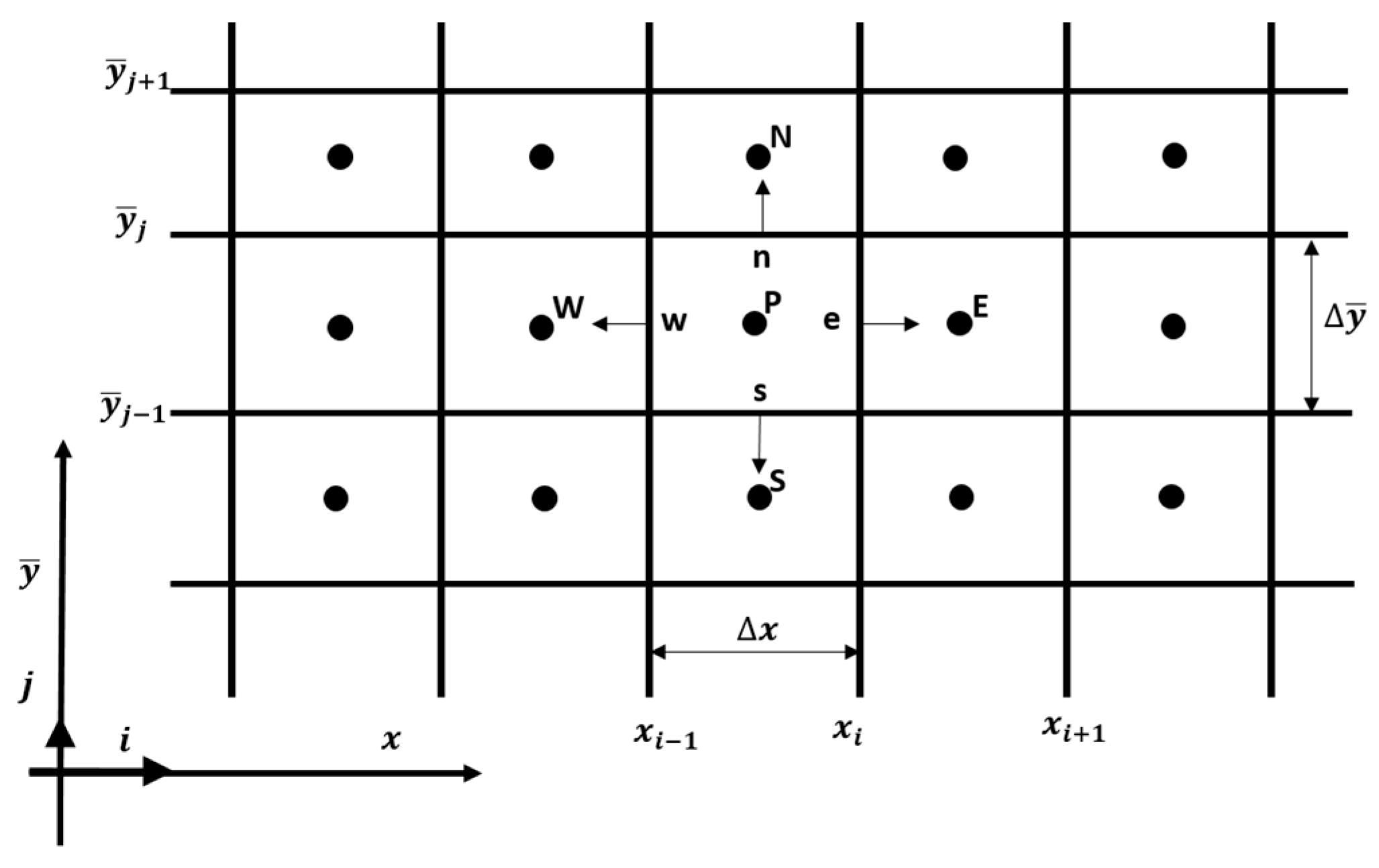
The slider is discretized with 2D computational cells as depicted in
Figure 2. Following the variable change described by Equation (2), the computational domain is rectangular and orthogonal. The computational cells have four plane faces, denoted by lower-case letters corresponding to their direction (e, w, n, and s) with respect to the central node P.
In the natural discretization numerical approach, the energy equation is solved using the finite volume method [
7]. Equation (3) is therefore integrated over the control volumes corresponding to the 2D computational cells:
For example, the convection transport terms in the
x direction can be expressed as:
An upwind discretization technique is used for the convective transport terms to avoid numerical instabilities [
7]. For example, at the east face of the control volume, the temperature
is up-winded based on the fluid flow direction. Mathematically, this can be expressed as:
This yields the discretization form of Equation (3):
where:
As stated in the introduction, the goal of the present work is to investigate the accuracy of the numerical solution of the energy equation given by the NDM and LPCM methods. Therefore, in order to avoid the uncertainties introduced by the numerical solution of the Reynolds equation, its analytic solution for the 1D slider is used.
Several other simplifying assumptions are needed for decoupling the Reynolds and the energy equations. Thus, the viscosity is considered constant and the flow regime laminar. Following the analytical solution, the pressure and the velocity in the 1D slider are [
1]:
The velocity
component across the thin film is deduced by integrating the continuity Equation (11) over the film thickness:
With the boundary conditions
and
, this yields:
It is to be underlined that in the following approach only the boundary condition at is used, while the second boundary condition at is used to check the accuracy of the numerical integration.
The discretized system given by Equation (7) is solved using any numerical procedure for a linear system with a positive definite matrix. Grids with 80 equidistant cells in the
x direction and different numbers of cells across the film thickness were used. The number of equidistant grid cells across the film thickness are
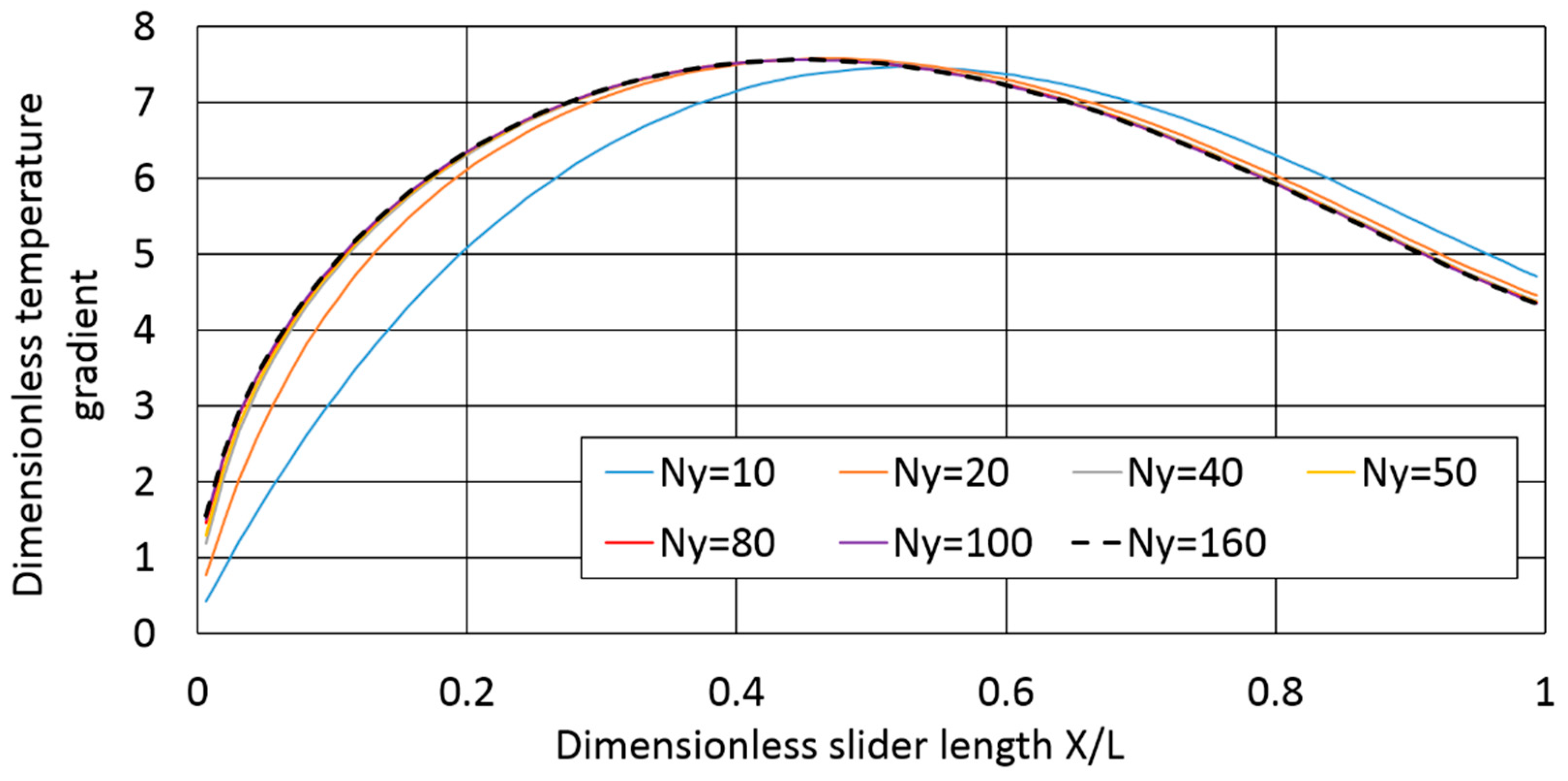
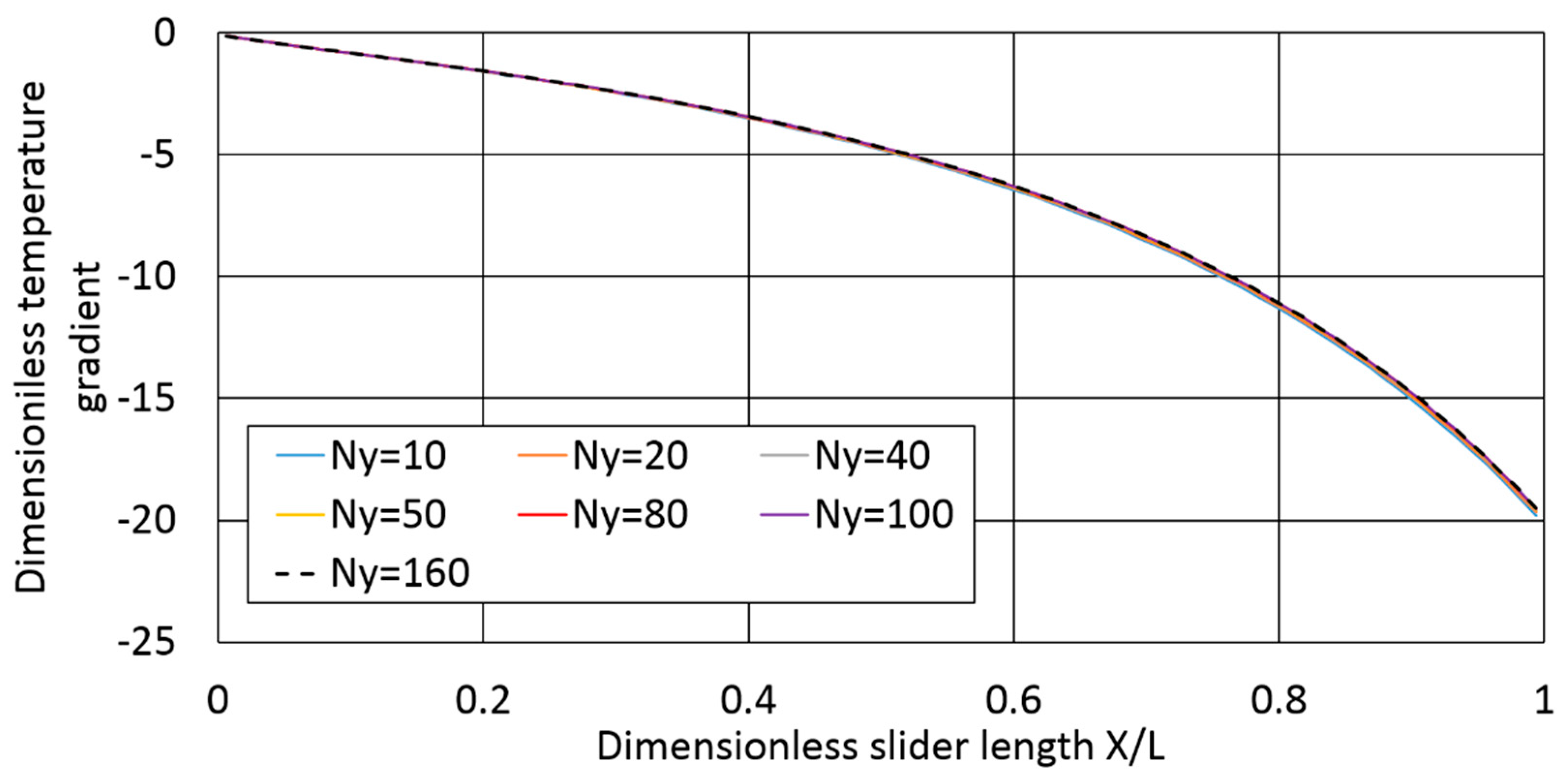
Ny = 10, 20, 40, 50, 80, 100, and 160. In a first test, the ambient temperature of 20 °C was imposed on the lower and upper walls and at the inlet. The dimensionless wall temperature gradient was monitored (This is equivalent to monitoring the wall heat fluxes). This dimensionless wall temperature gradient is defined by:
where
is a reference temperature.
The results are depicted in
Figure 3 and
Figure 4, and show that the curves become superposed starting with
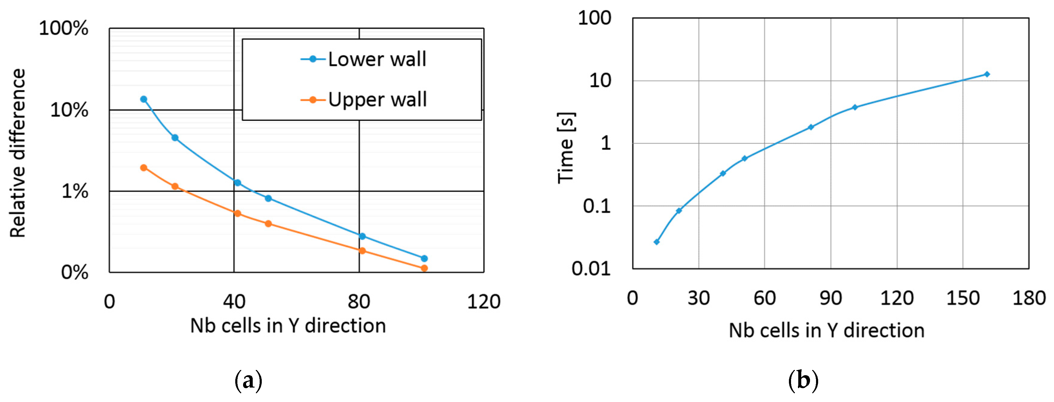
Ny = 40 cells. An estimation of the accuracy is obtained by using the relative difference of the wall temperature gradients which is defined in Equation (14):
where
is the solution obtained with the finest grid
Ny = 160.
The variation of these errors with the number of grid cells across the film thickness is depicted in
Figure 5a, and the computational time is depicted in
Figure 5b. A rapid increase in the computational time with the grid cells must be underlined. For example, the calculation case with
Ny = 80 grid cells required 1.844 s, while the computational time for the case with
Ny = 160 cells was one order of magnitude higher. However, for the purpose of accuracy, the mesh with
Ny = 160 was chosen as the reference solution in the following and its numerical values of the wall temperature gradients are given in
Table A1 in
Appendix B.
3. The Numerical Solution of the Energy Equation Based on the Lobatto Points Collocation Method
The Lobatto Point Collocation Method (LPCM) is based on the approximation of the temperature with Legendre polynomials across the film thickness. Because Legendre polynomials are defined on the interval
, the following coordinate transformation is used:
where
is the new dimensionless coordinate across the film thickness.
Following the coordinate transformation, the energy Equation (1) becomes:
For an incompressible lubricant with constant viscosity, only the variable temperature
is approximated across the film thickness:
where
is the highest order of the Legendre polynomials,
is the Legendre polynomial of degree
j, and
is the polynomial coefficients of temperature of degree
j.
This description holds for every point in the 2D computational domain. Compared to the NDM, which computes directly the temperature by solving the energy equation discretized over the film thickness, the LPCM calculates the polynomial coefficients of temperature
. Based on the work of Mahner et al. [
6], the coefficients of the Legendre polynomials expansion can be obtained using different methods, but it is accepted that the most reliable is the collocation method using the Lobatto points. The Lobatto points are the roots of the derivative of the Legendre polynomial of the highest degree (i.e., the roots of
).
For a given position in the x direction, the temperature is replaced by its approximation from Equation (17) across the fluid film, and the energy Equation (16) is enforced to hold true for each Lobatto point, . This leads to N − 1 partial differential equations with the unknown . The boundary conditions are applied at the two walls, and , which leads to the other two equations. In total, a system of N + 1 equations for the N + 1 unknown is obtained.
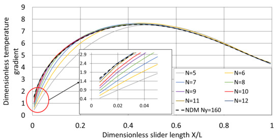
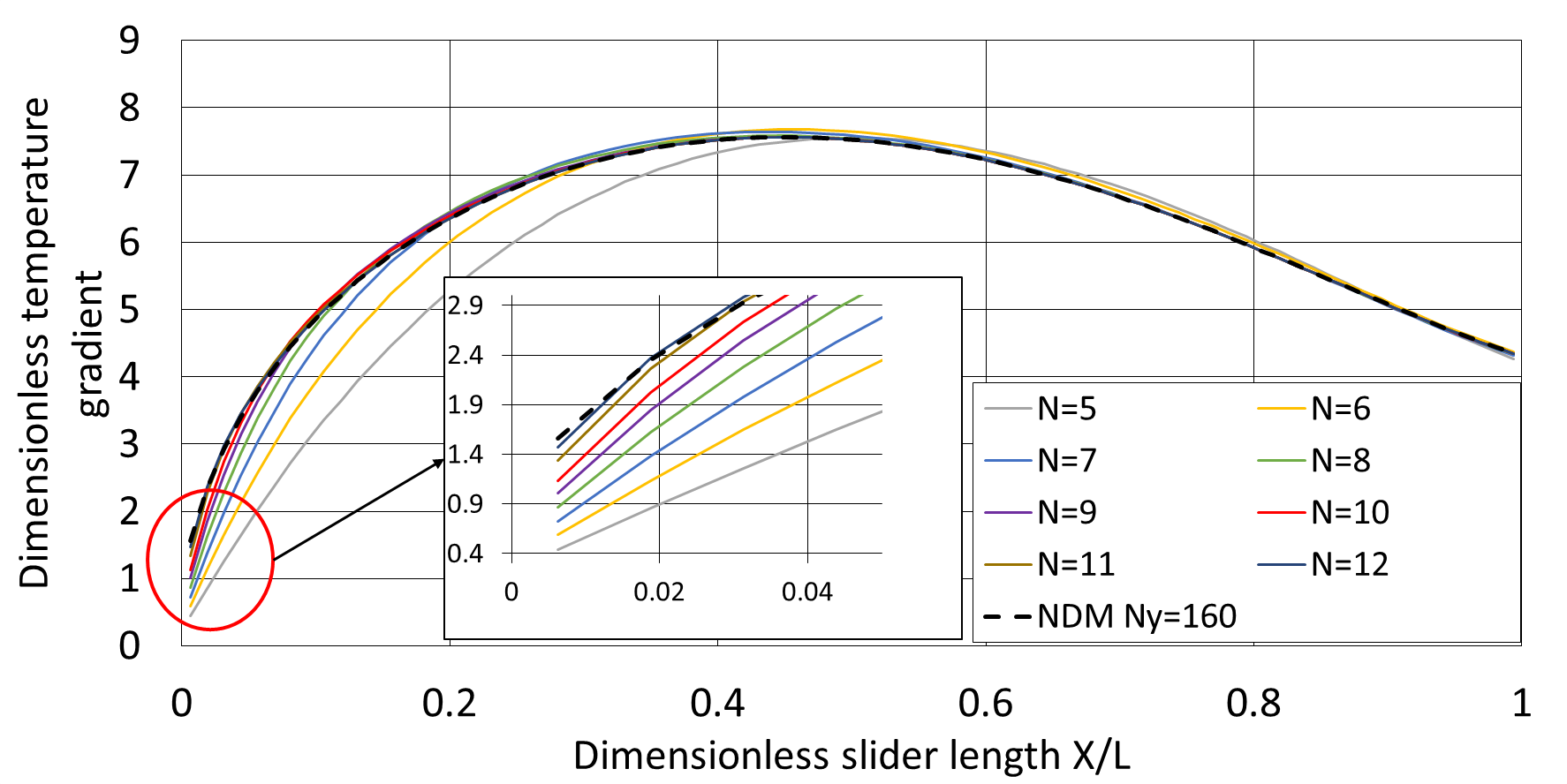
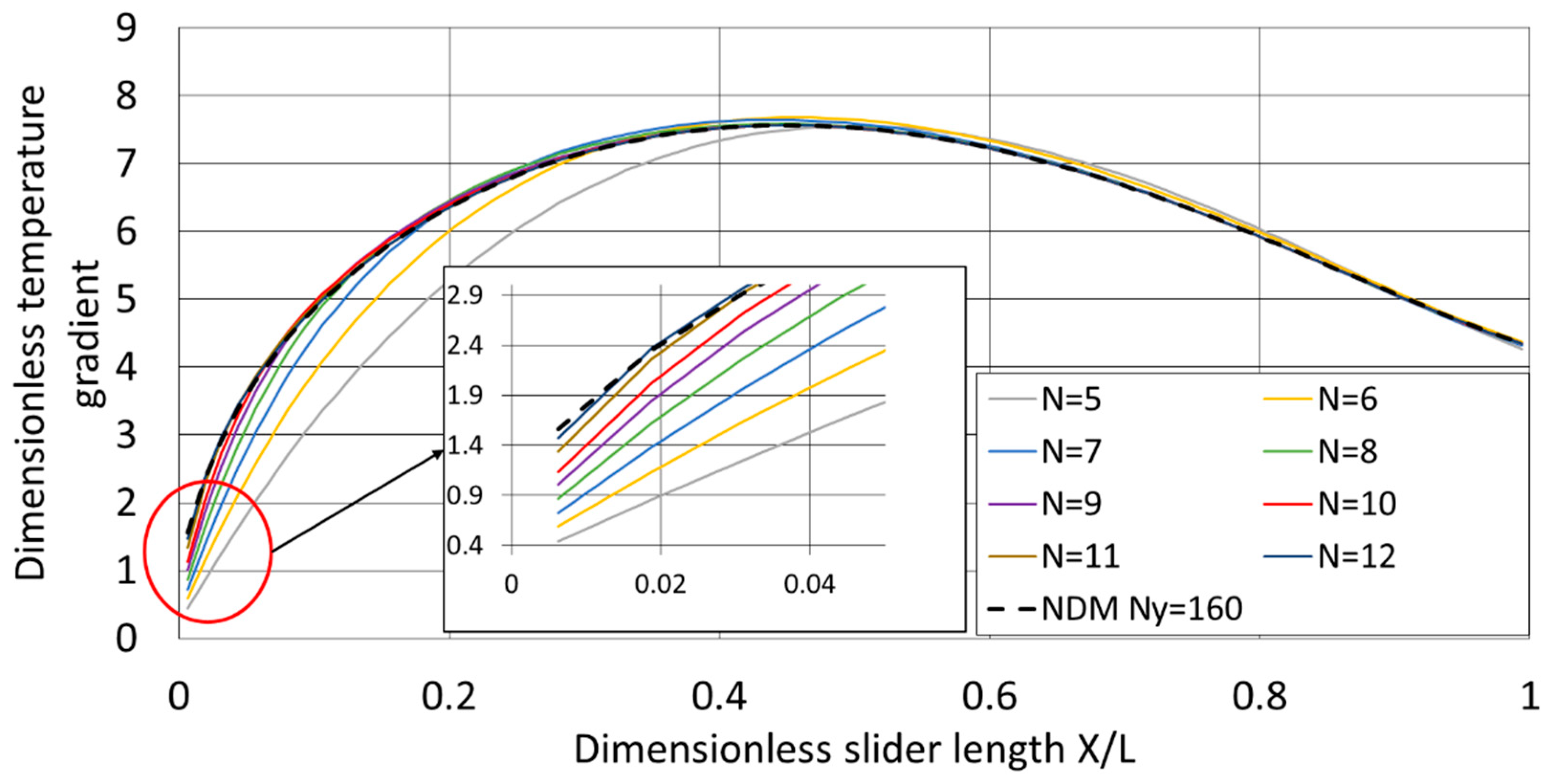
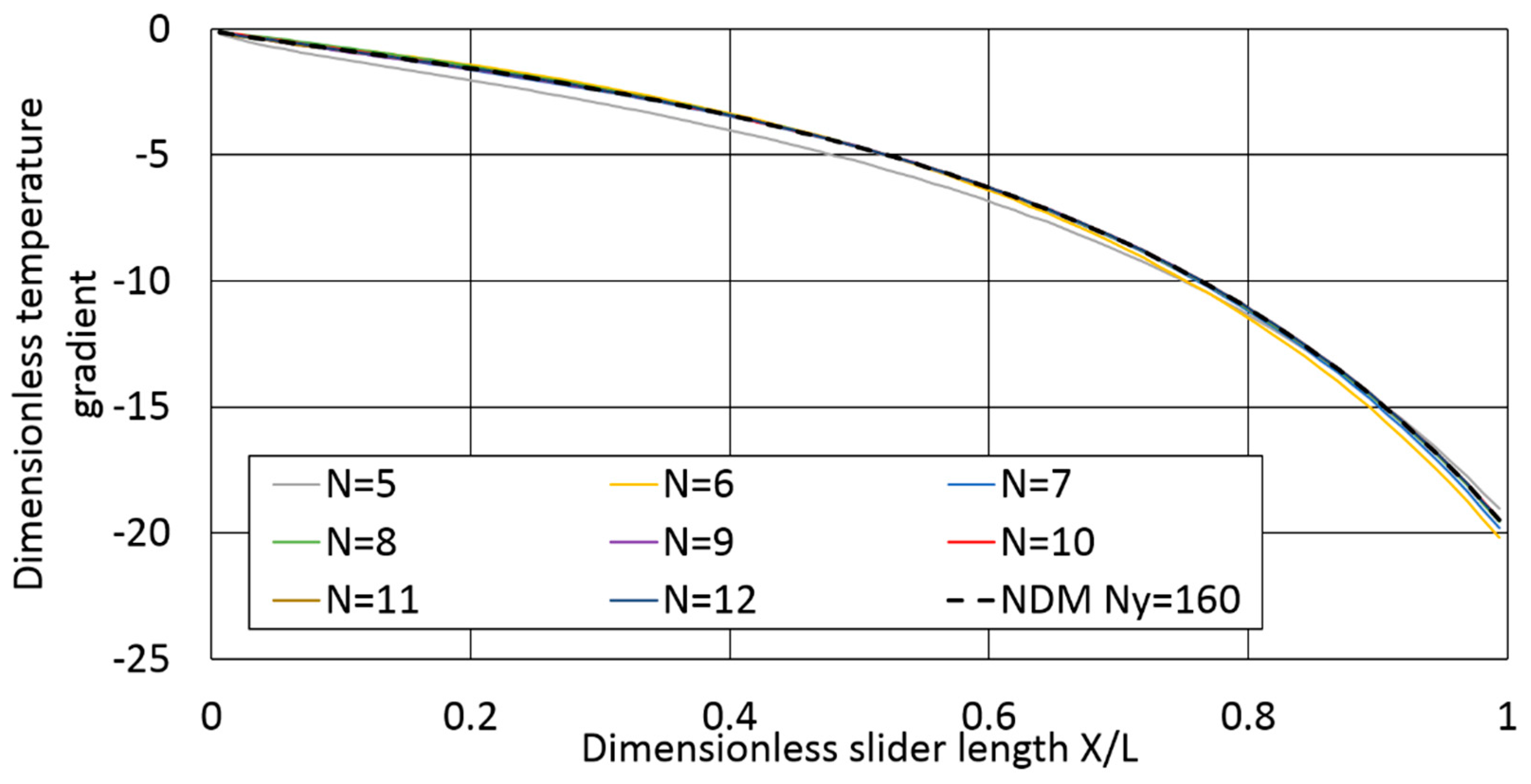
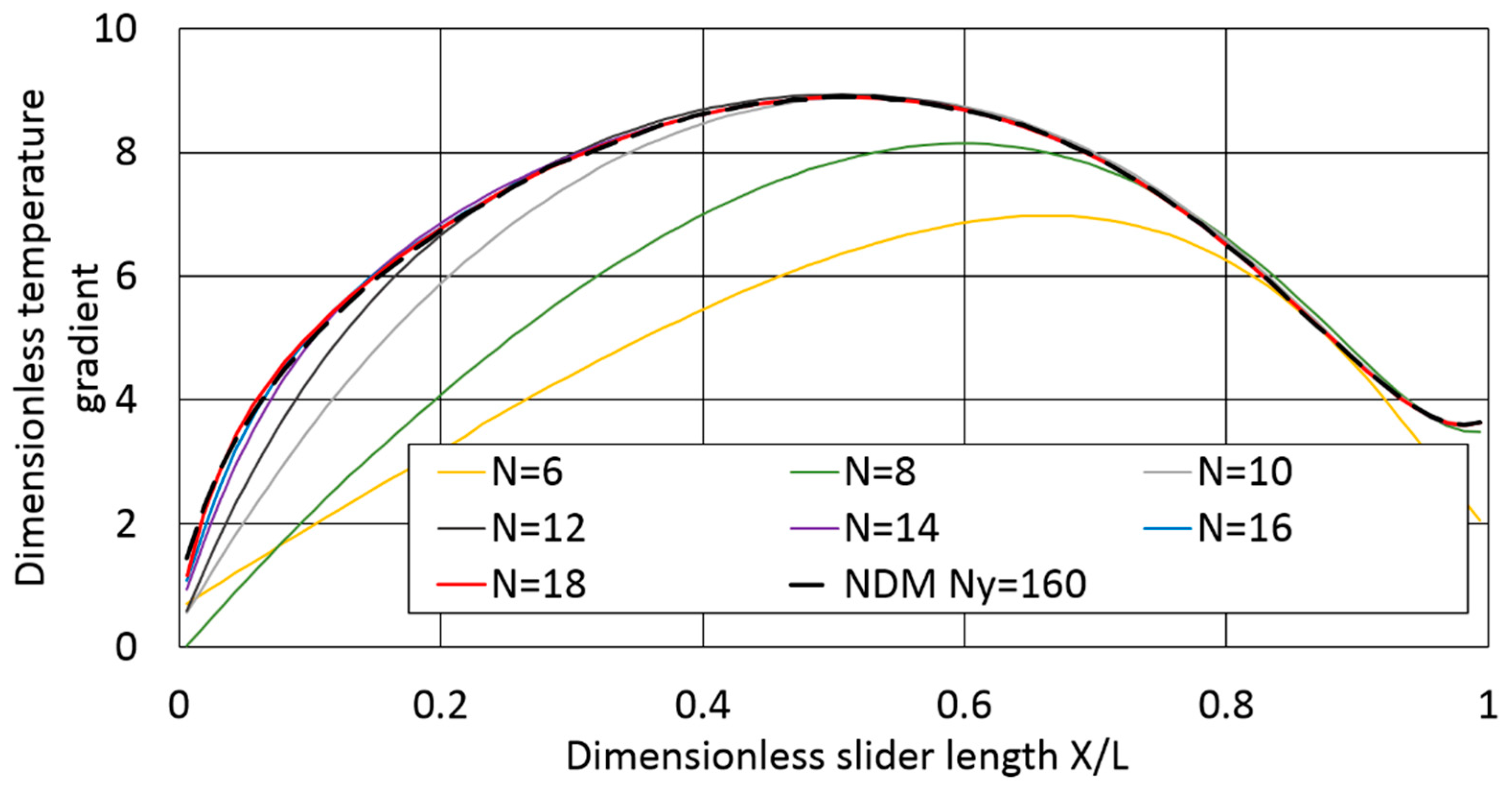
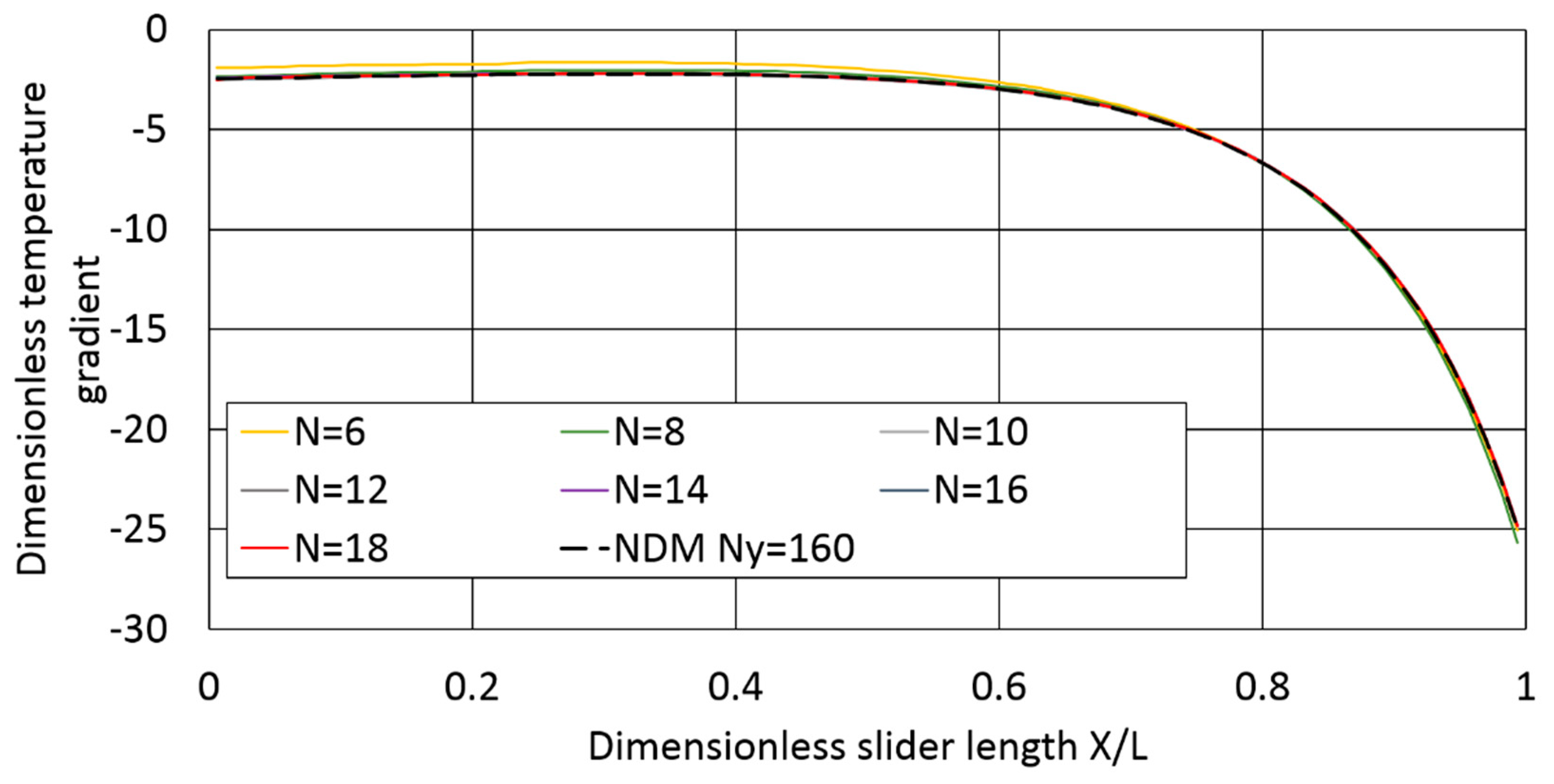
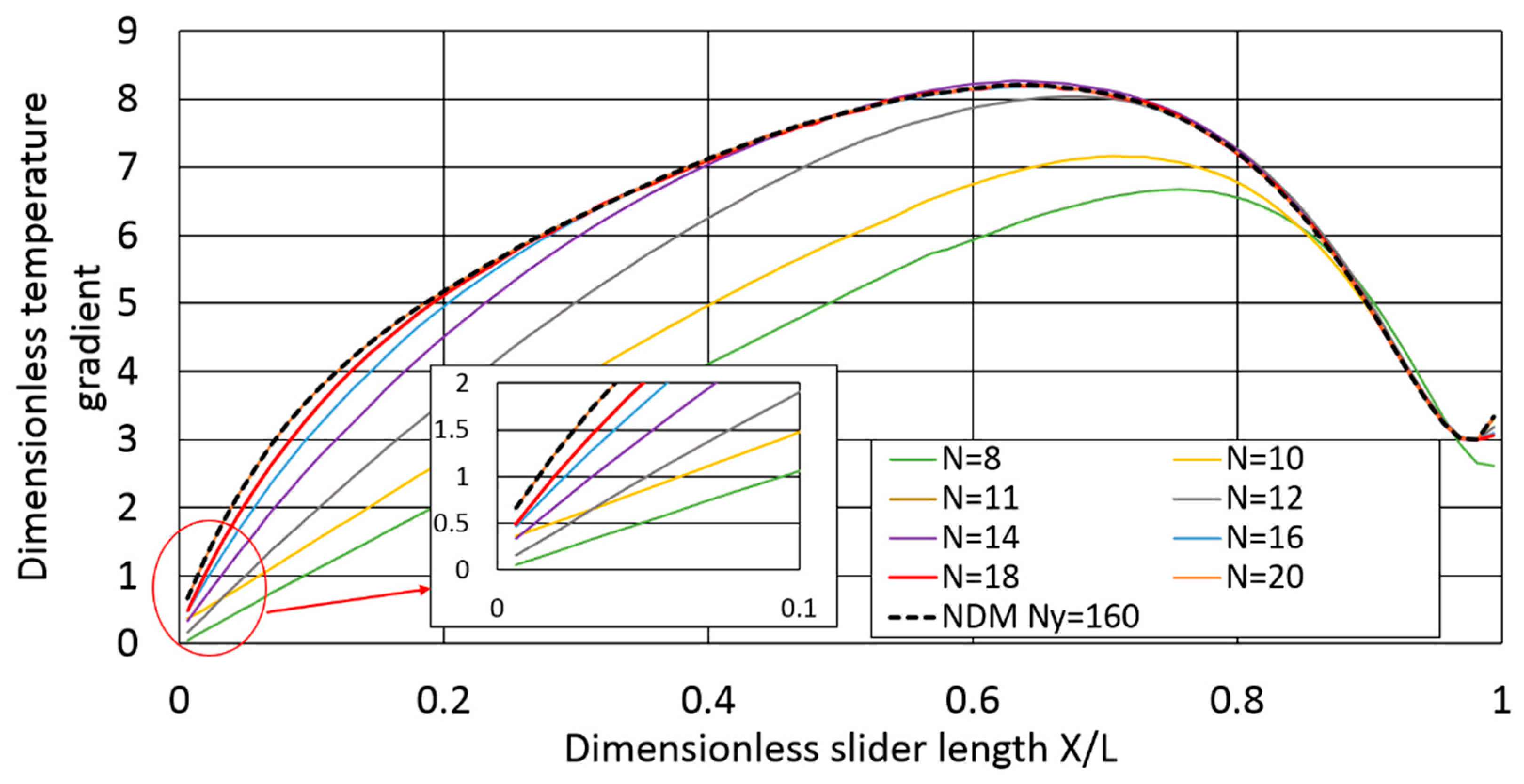
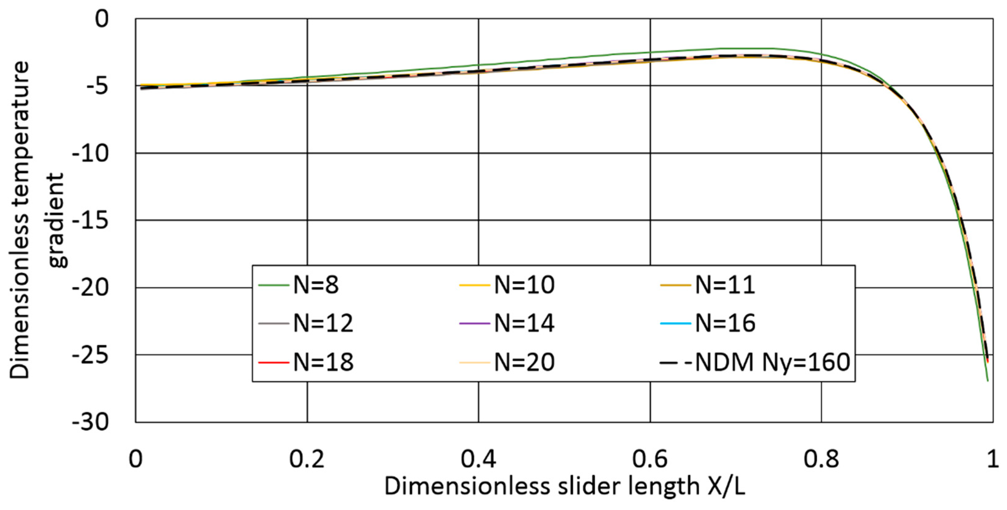
Figure 6 and
Figure 7 depict the dimensionless wall temperature gradient obtained with an increasing degree of the Legendre polynomials. The difference between the NDM solution and the LPCM solution at the lower wall (
Figure 6) in the inlet section is reduced by increasing the degree of the Legendre polynomial.
The reference results used for comparison are given by the NDM with
Ny = 160 grid cells. The relative difference between the reference results and the wall temperature gradient obtained with the LPCM is defined as:
where
or
for LPCM, and
or
for NDM.
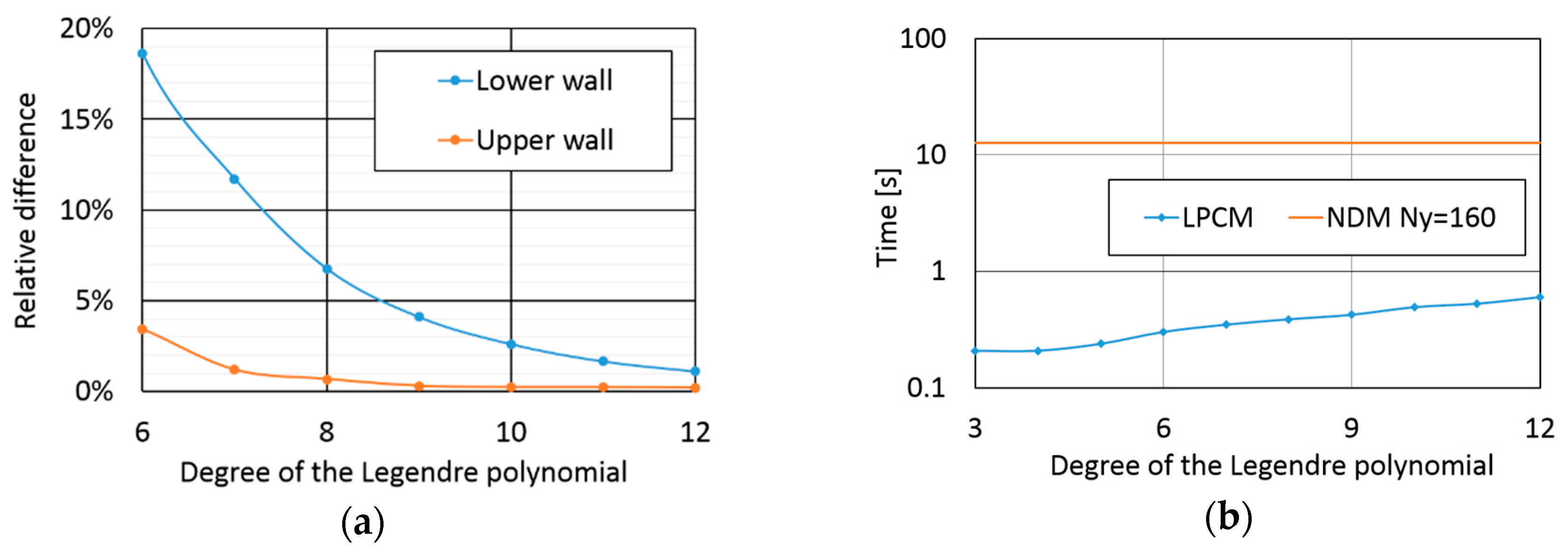
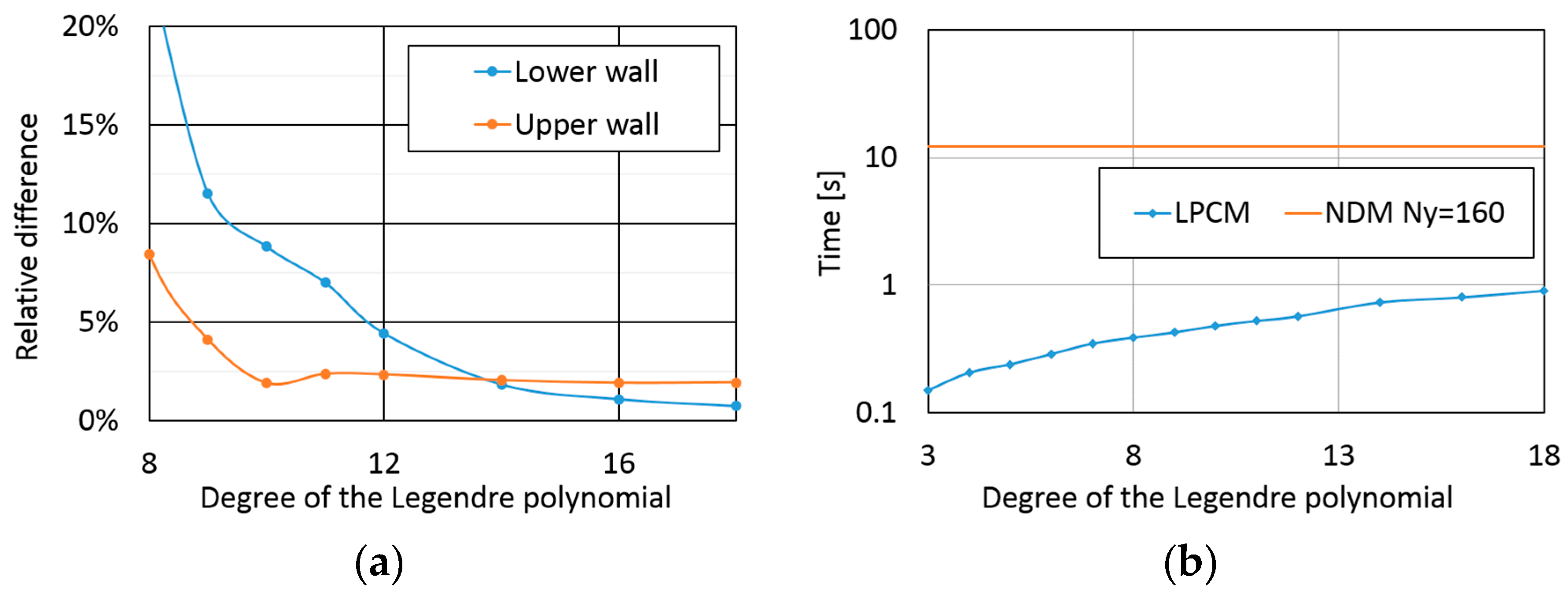
The relative difference is depicted in
Figure 8a. This relative difference decreases rapidly with the increase of the degree of the Legendre polynomial. However, the lower and upper wall results show different trends. A higher degree of the Legendre polynomial is required to reach a grid independent solution at the lower wall. This is due to the more predominant thermal effect at the driving wall; that is, the lower wall.
The computational effort is depicted in
Figure 8b. Compared with the reference solution, the computational time of the LPCM solution is divided by ten, since only a limited expansion of the Legendre polynomials is necessary to obtain grid independent results.
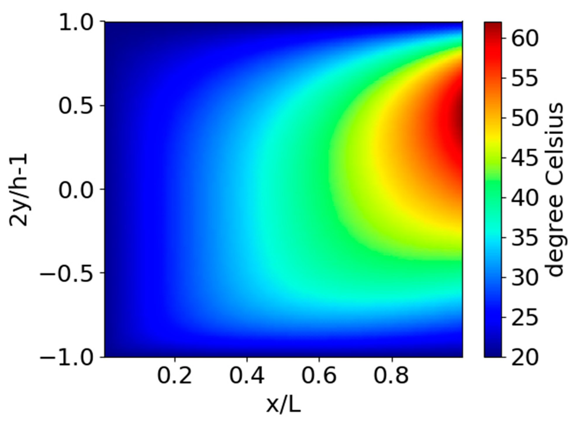
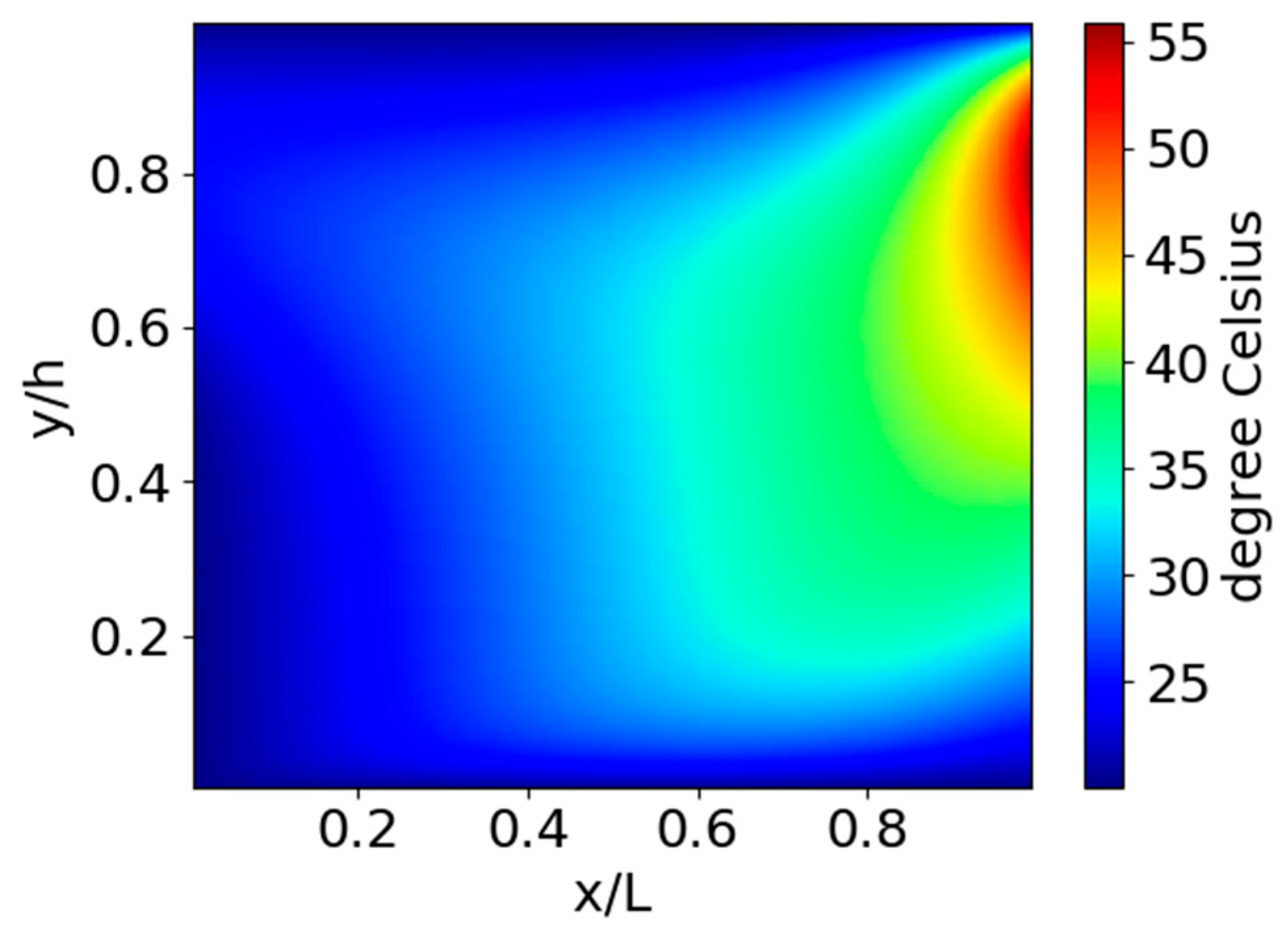
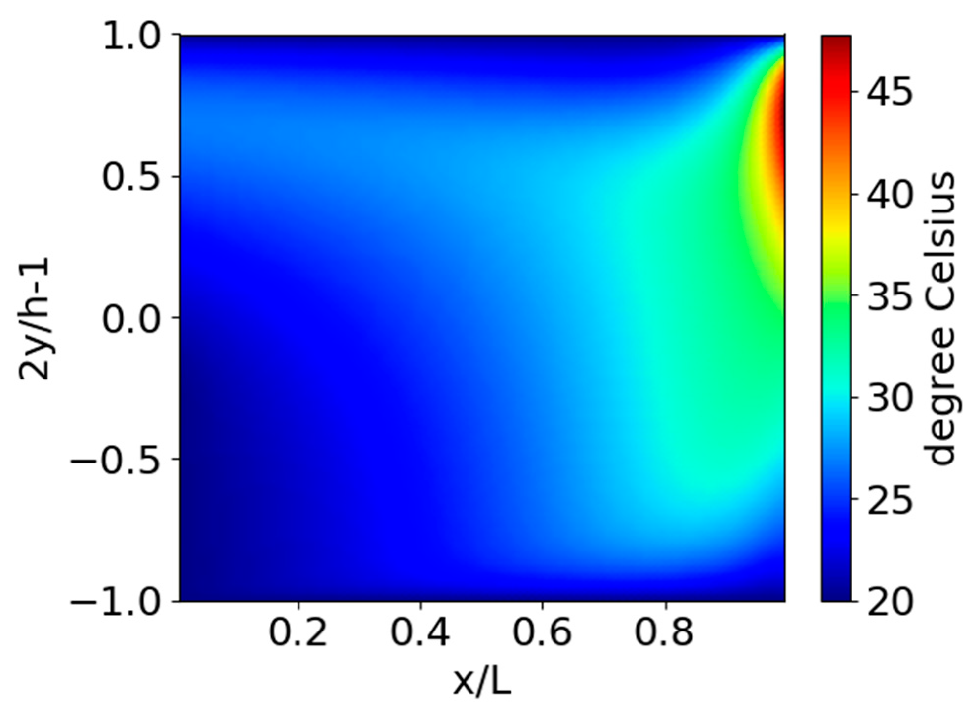
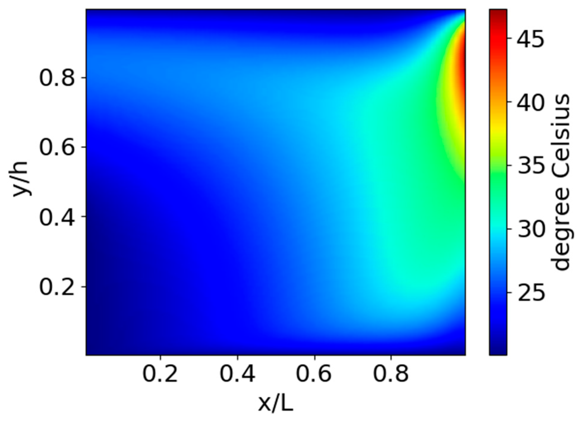
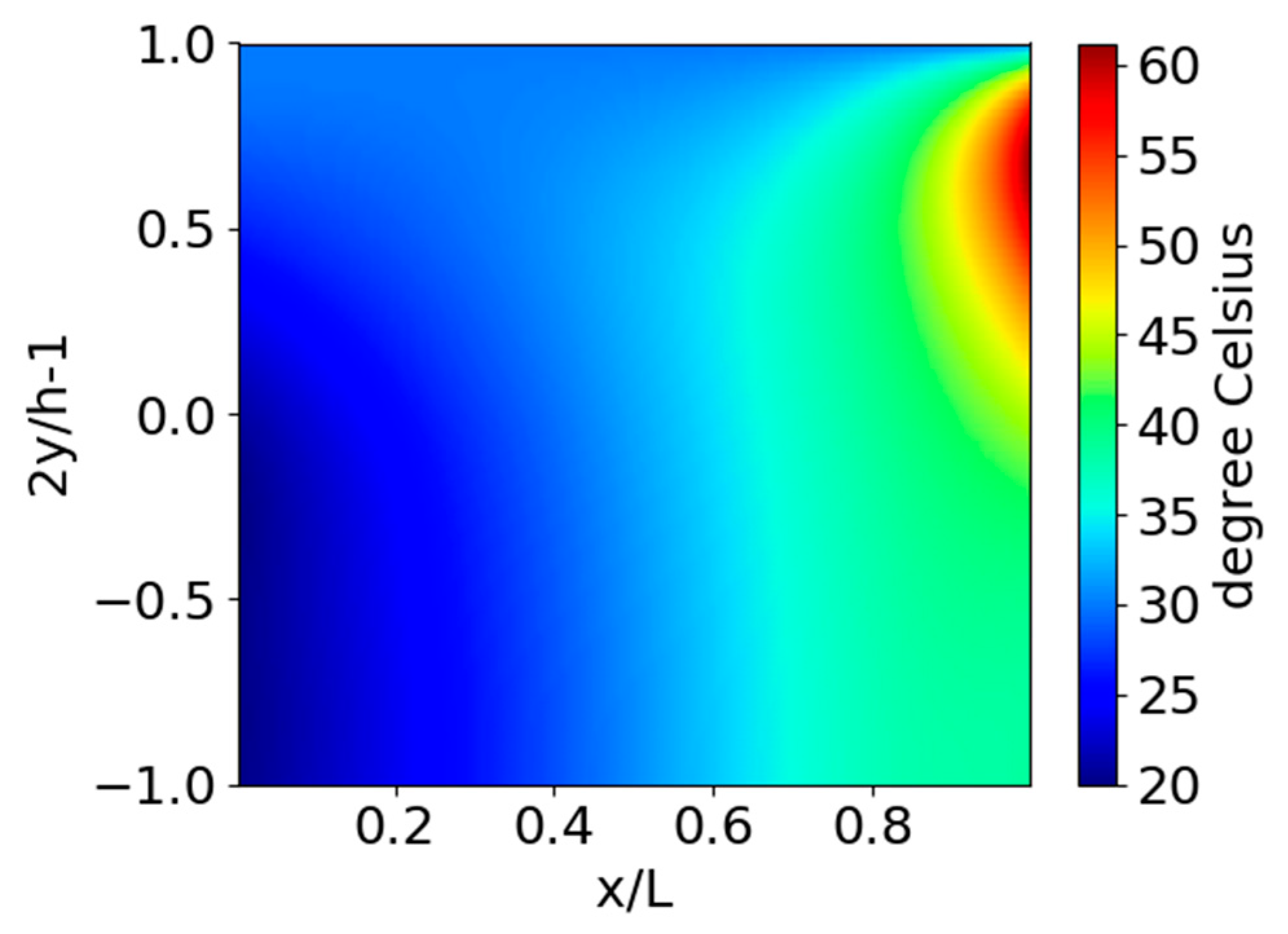
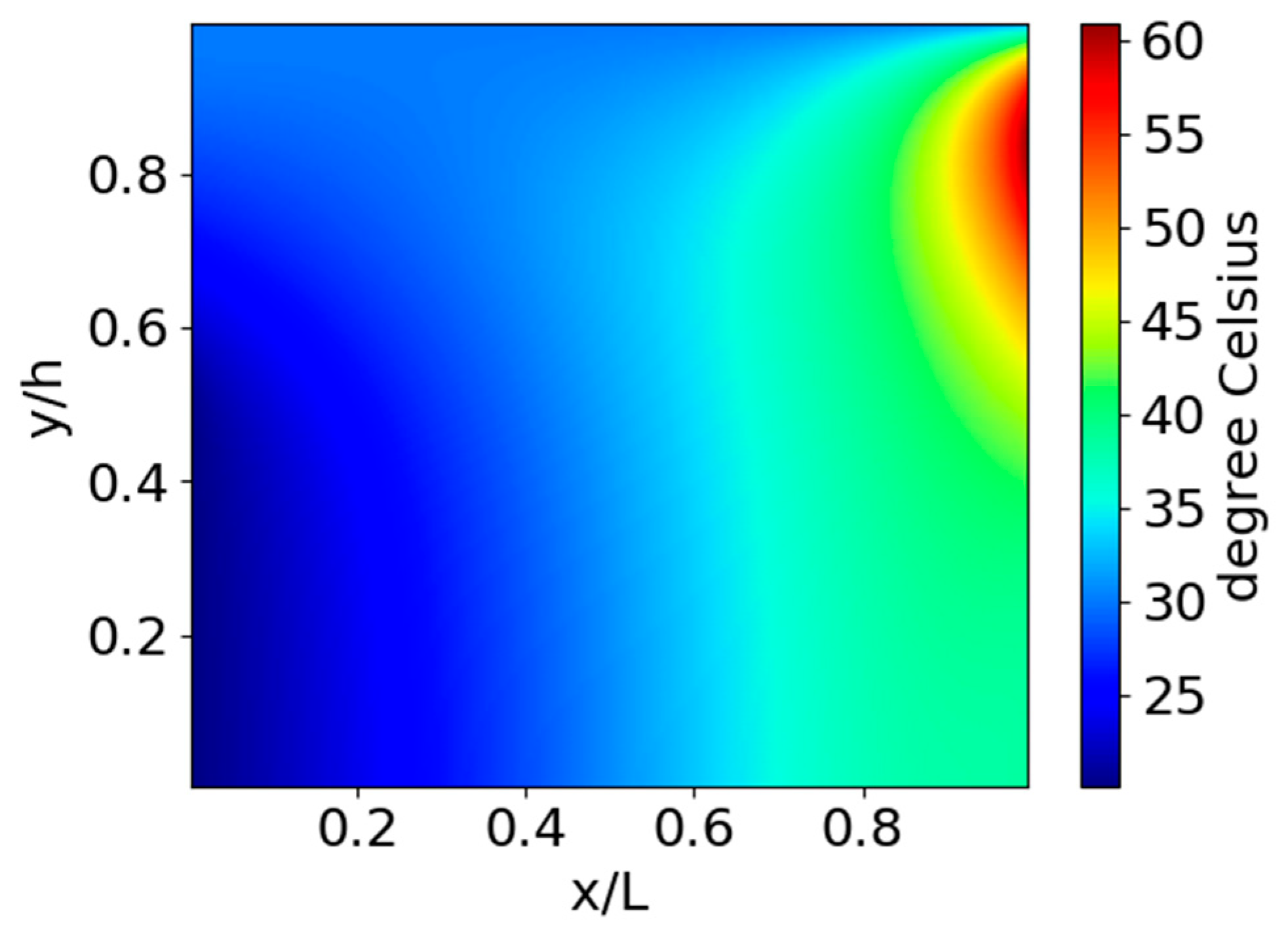
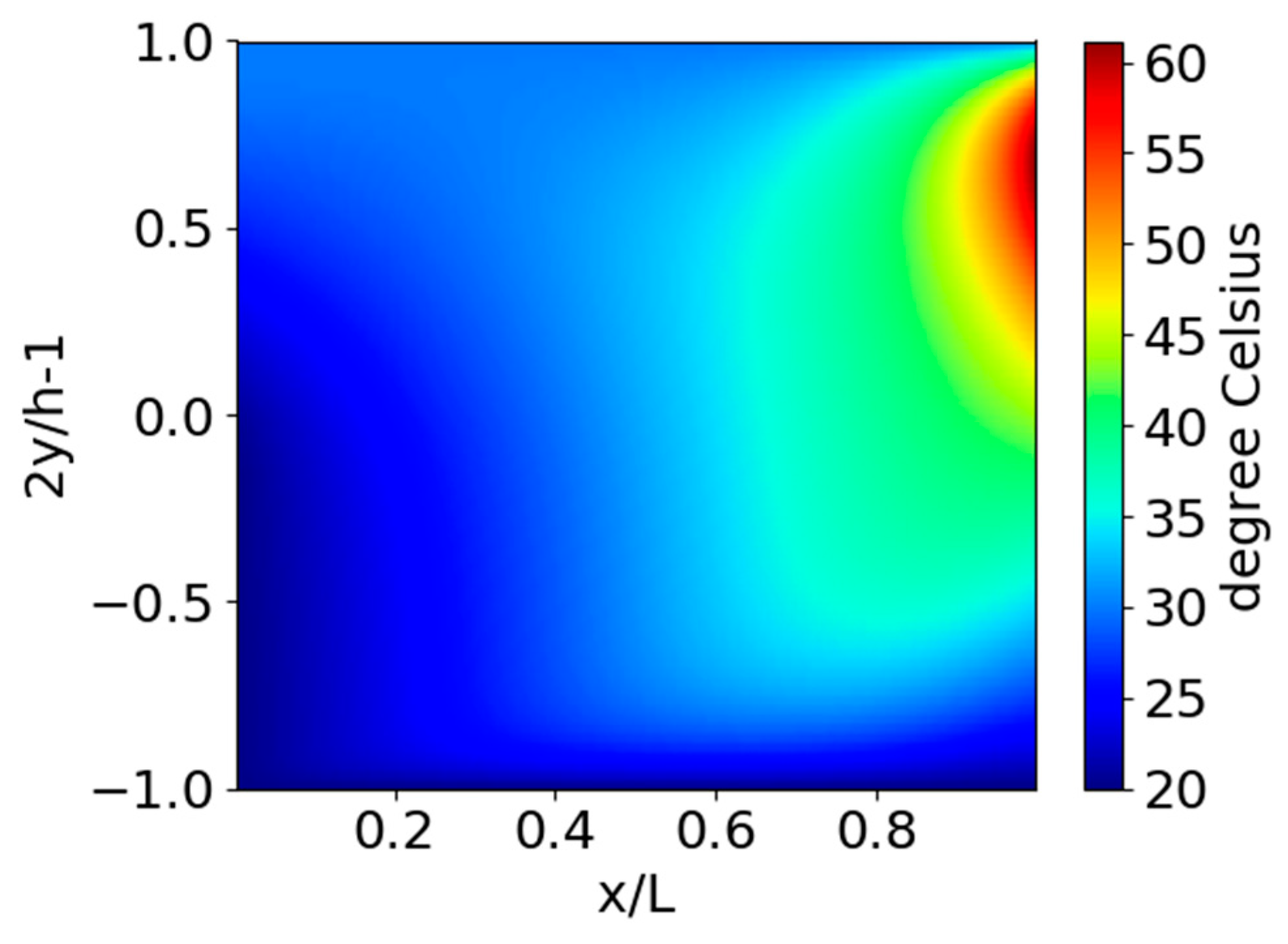
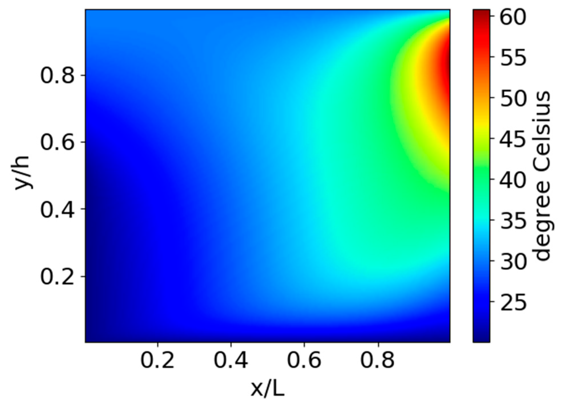
For comparison, the temperature fields obtained with the LPCM (
N = 12) and the NDM (
Ny = 160) are depicted in
Figure A1 and
Figure A2 in
Appendix A, respectively. The obtained polynomial coefficients of temperature of degree
j,
, are given in
Table A2 in
Appendix B. The present analysis indicates that the LPCM results are more accurate for the same grid density.
4. Further Comparison of Numerical Results Obtained by NDM and LPCM
The previous results were obtained for a linear converging 1D slider with an inlet/outlet film thickness ratio h1/h2 = 2, imposed wall temperatures (Dirichlet boundary condition), and completely decoupled from the Reynolds equation. Other simple cases of the converging 1D slider were also investigated and bring interesting conclusions.
4.1. Different Geometrical Configurations of the 1D Slider
Two other inlet/outlet film thickness ratios, h1/h2 = 4 and h1/h2 = 8, were investigated while keeping the same wall temperature boundary conditions and the decoupled Reynolds equation. The increased inlet/outlet film thickness ratio leads to a slower convergence of the NDM results with the y grid refinements. The best NDM solution obtained with Ny = 160 was considered as the reference results, and the number of computational cells in the x direction was kept the same (Nx = 80 cells).
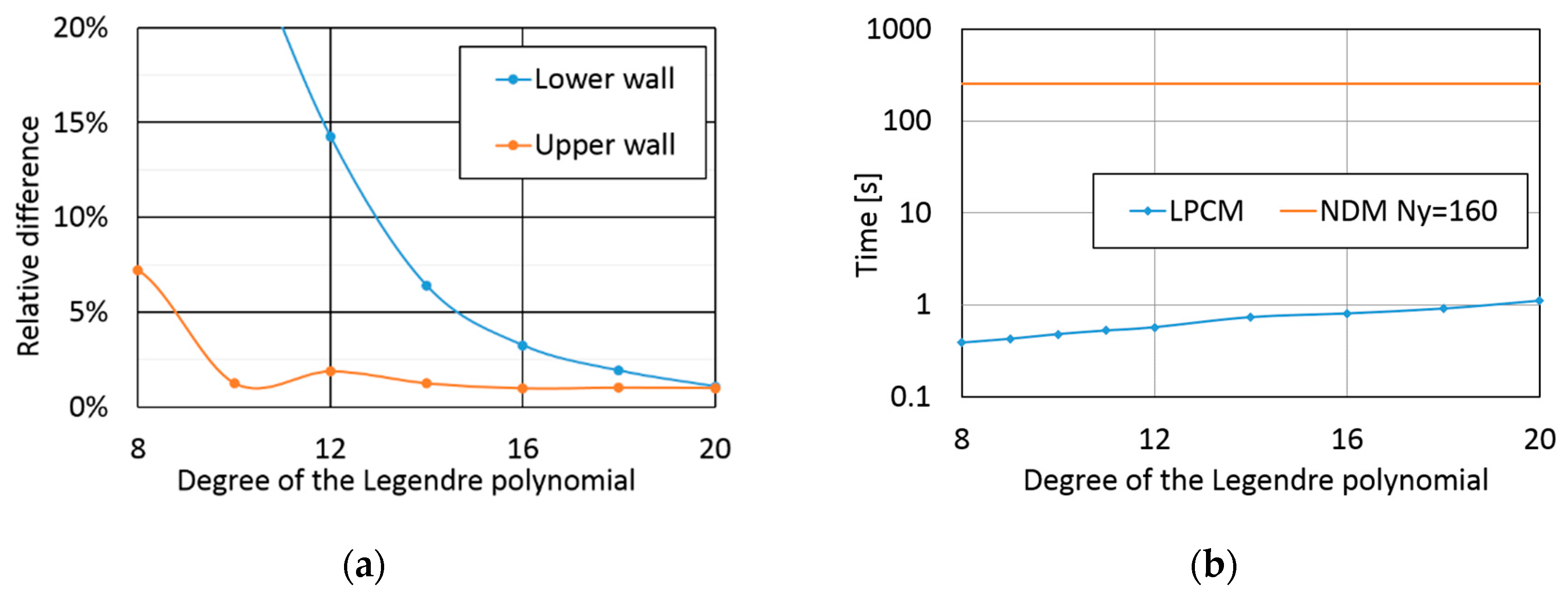
The results obtained for
h1/
h2 = 4 are depicted in
Figure 9,
Figure 10 and
Figure 11. Again, the lower and upper wall results show different trends. The upper wall temperature gradient reaches grid convergence starting with the Legendre polynomials of 11 degrees, while the resolution of the lower wall gradient needs
N = 16 Legendre polynomials. However,
Figure 11b shows that even when using a high number of Legendre polynomials, the LPCM requires one order of magnitude less computational time than the NDM for the same accuracy.
The results obtained for
h1/
h2 = 8 are depicted in
Figure 12,
Figure 13 and
Figure 14. The same remarks as for
h1/
h2 = 4 can be drawn, except for the fact that this time, a higher order of the Legendre polynomials was needed for the grid convergence solution, and this is related to the increased inlet/outlet film thickness ratio.
Figure 14b shows that the computational time of the NDM with
Ny = 160 increases for this calculation case. It can be seen from
Figure 11b and
Figure 14b that the computational effort of the NDM increases one order of magnitude with increasing the ratio
h1/
h2 from 4 to 8. This was not the case for the LPCM, which required the same computational time for these two cases, one or two orders of magnitude lower than the NDM. Therefore, LPCM remains largely superior to NDM in terms of the computational time.
4.2. Different Thermal Boundary Conditions Applied to 1D Slider
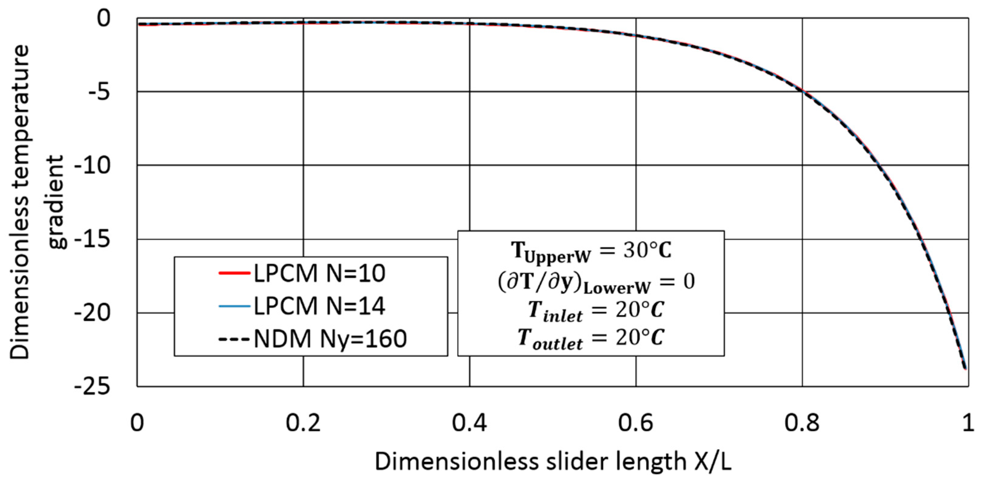
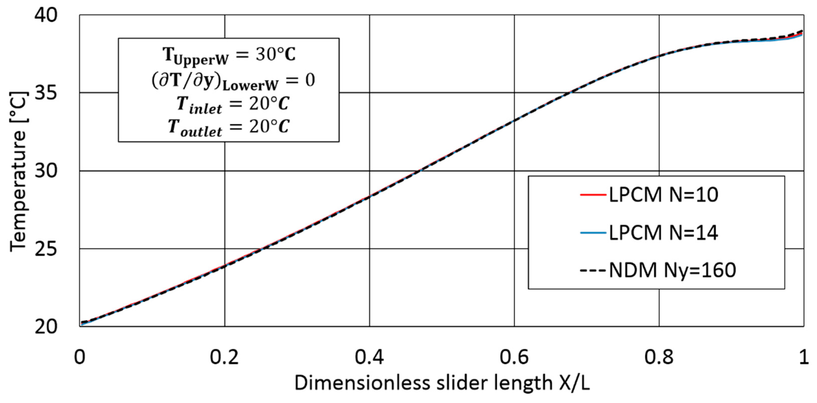
The previous cases dealt with imposed wall temperatures, while the wall temperature gradient was a calculation result. In the following test, the lower wall of the 1D slider was adiabatic; that is,
while the temperature of the upper wall is
. The film thickness ratio is
h1/
h2 = 4 and the inlet temperature
. For the LPCM, 10 and 14 Lobatto points were used and the results were compared to the NDM (
Nx = 160 cells and
Ny = 160 cells, all equidistant).
Figure 15 and
Figure 16 show the consistent resolution of the upper wall temperature gradient and of the lower wall temperature.
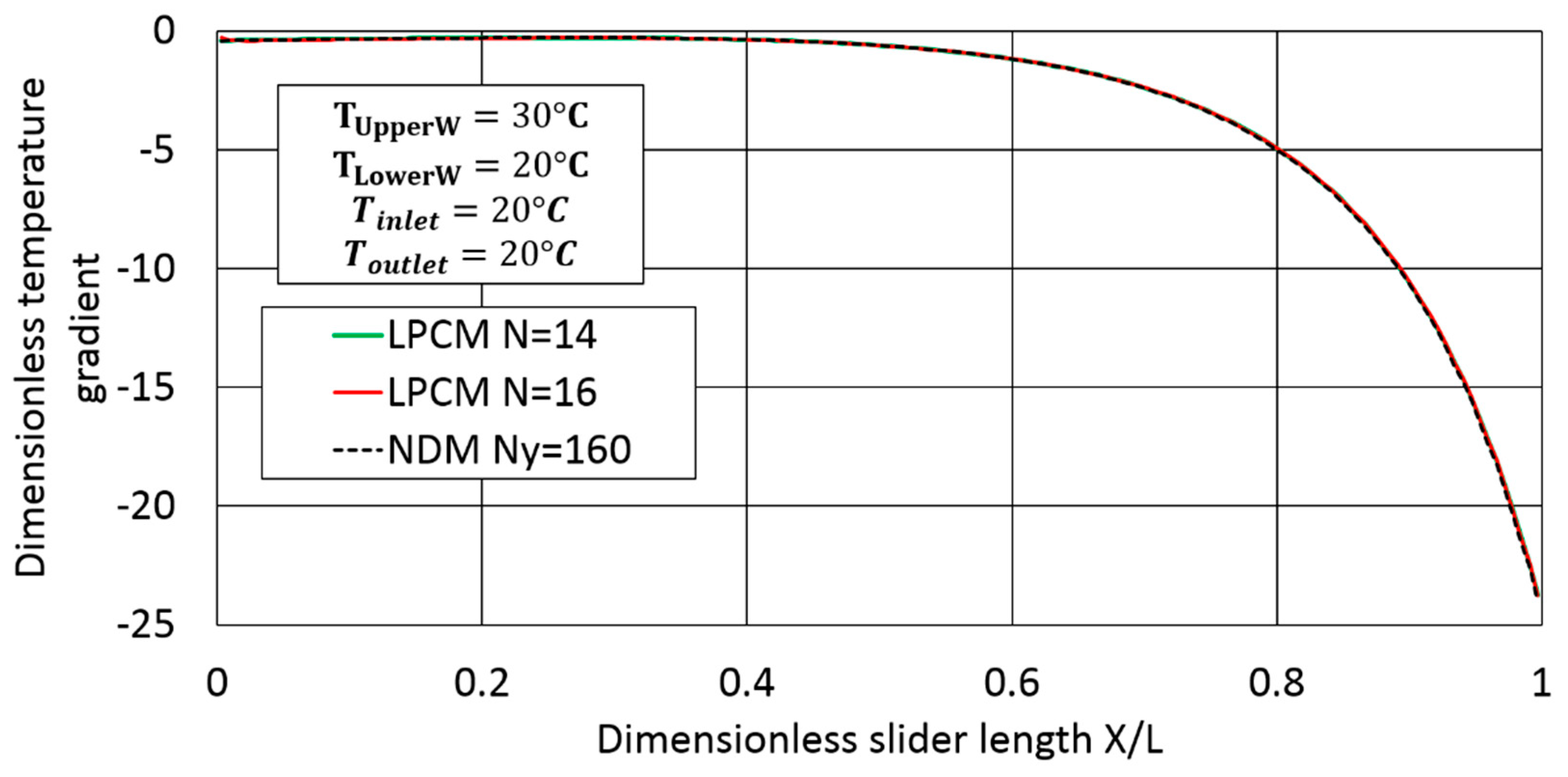
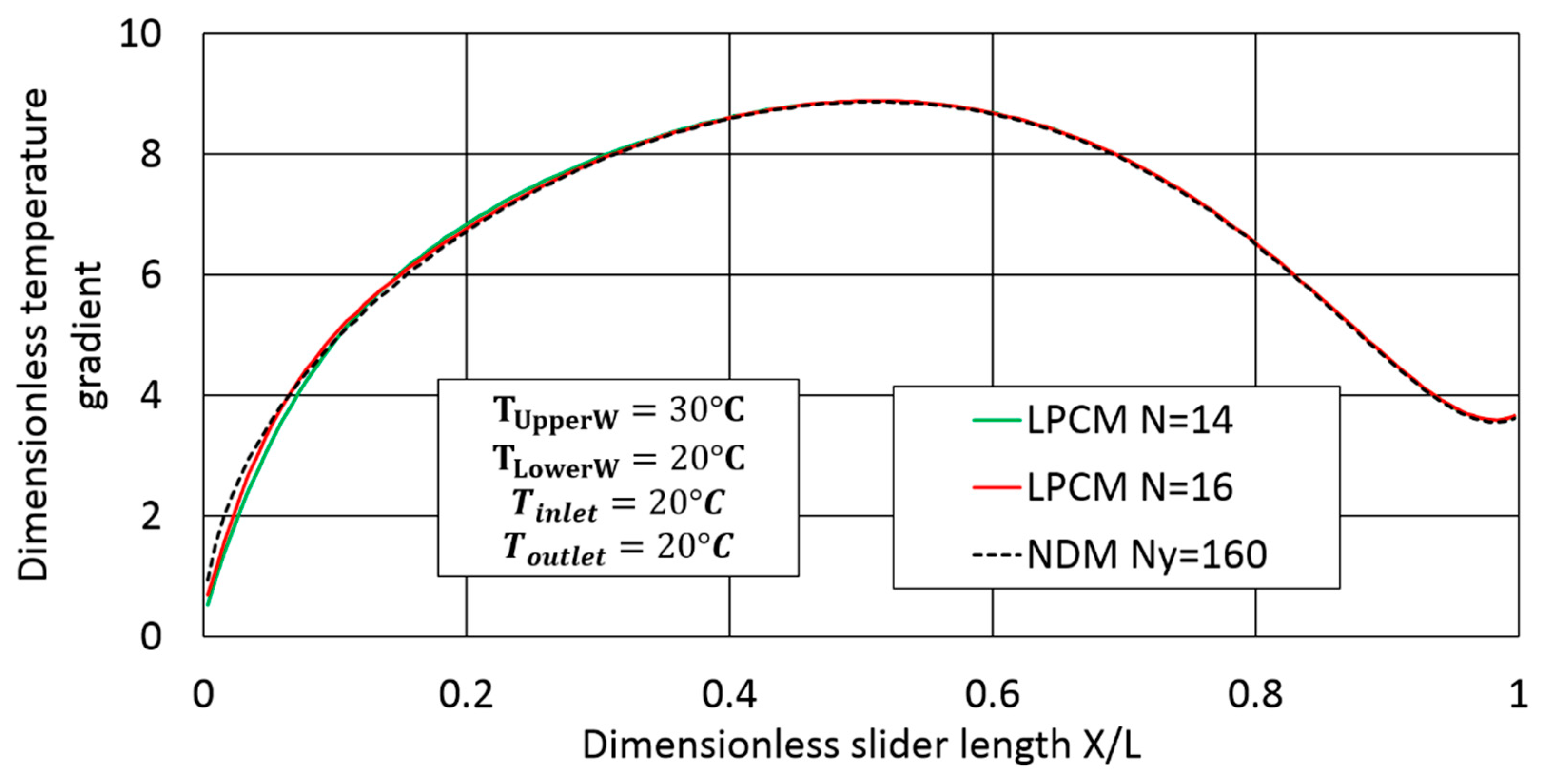
A different test case consists of imposing different wall temperatures,
,
, and
. The LPCM was performed with 10 and 14 Lobatto points, and the previous resolution was used for the NDM. The results are depicted in
Figure 17 and
Figure 18, and show that discrepancies exist between the NDM solution and the LPCM solution at the lower wall (
Figure 18) in the inlet section. Again, this difference is reduced with the increase of the degree of the Legendre polynomials. It is necessary to highlight that the LPCM method approximates the temperature gradient at the walls based on the polynomial coefficients of temperature over the film thickness, while the NDM method calculates the temperature gradient with finite differences over a limited number of boundary cells. Thus, the two methods have different approximation orders. In some extreme configurations, it is necessary to increase the degree of the Legendre polynomial in order to reach the grid independent solution.
5. Results for the Energy Equation Coupled with the Reynolds Equation
The above presented results showed the grid refinements required for obtaining accurate solutions of the energy equation when decoupled from the Reynolds equation. In reality, the viscosity of a liquid lubricant depends strongly on the temperature, and therefore decoupling is very difficult. For this reason, the data found in the literature always considered the complete thermo-hydrodynamic analysis.
This thermo-hydrodynamic (THD) coupled analysis was subsequently performed for the 1D slider case. The results of the LPCM were compared with the data from Ref. [
3]. Their grid convergence and the computational time were analyzed by comparisons with NDM results. This step completes the validation of the decoupled energy equation described in the previous sections.
A temperature dependent viscosity following an exponentially decaying law was used to replace the constant viscosity . The rest of the geometrical and physical parameters were the same as in the previous case. The inlet and wall temperatures were equal to the ambient reference temperature. As for the variations of the temperature across the thin film, the terms in the generalized Reynolds equation with variable viscosity were also discretized by Legendre polynomials, and the coefficients were obtained by collocation at the Lobatto points.
As for Ref. [
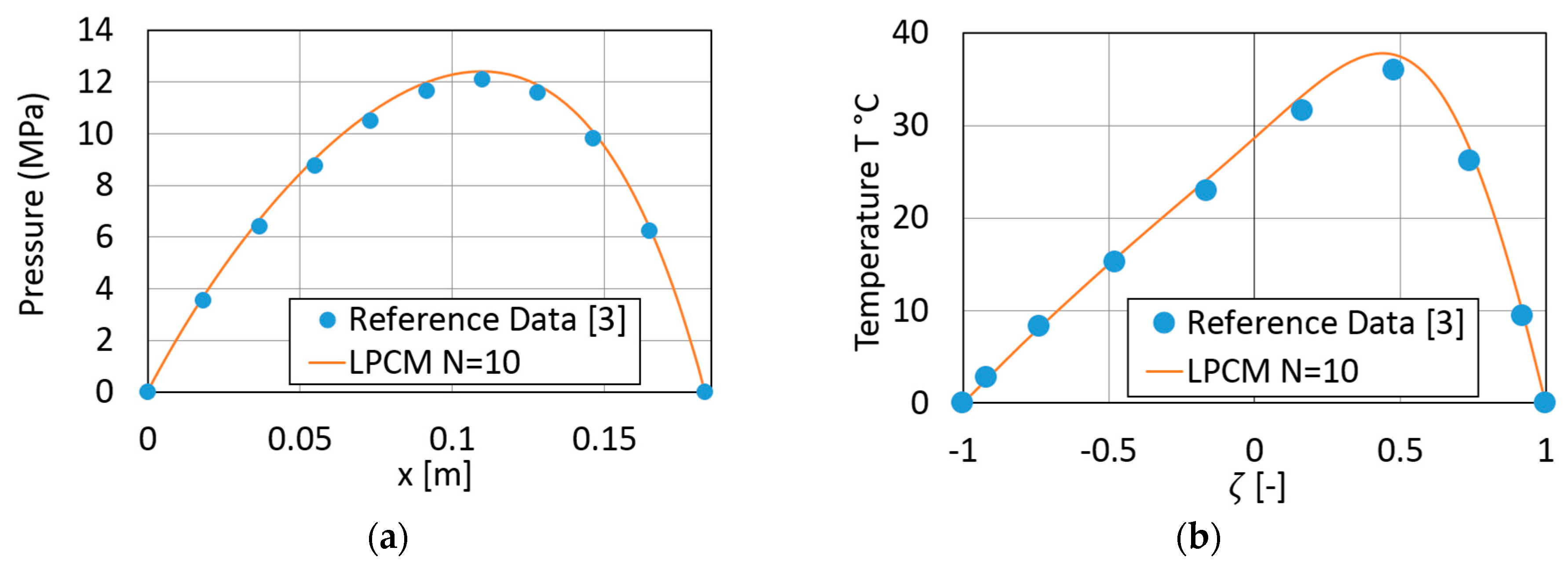
3], the computational domain of the 1D slider was discretized using
Nx = 30 equidistant cells in the main flow direction and 10 Lobatto points across the film thickness. The Reynolds and the energy equations were numerically solved following a segregated approach.
Figure 19a compares the pressure variation in the 1D slider obtained with the LPCM and the one given in Ref. [
3].
Figure 19b presents the variation of the outlet temperature difference across the film thickness. Both the pressure and the temperature variations obtained with the LPCM are in agreement with Ref. [
3].
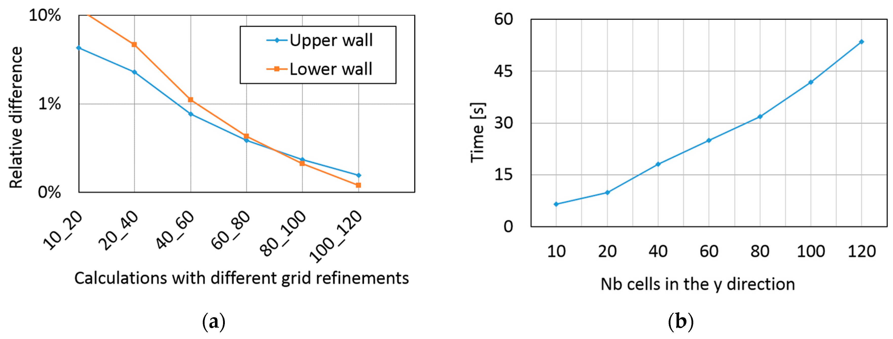
This 1D non-isothermal slider was also used to compare the efficiency of the LPCM with the NDM. Several calculations were performed with the NDM method in order to check the grid convergence and for obtaining results that could serve as a reference. These tests used seven grid refined in the
y direction (
Ny = 10, 20, 40, 60, 80, 100, and 120 equally spaced control volumes), while a constant number of 30 control volumes was used in the
direction. The relative difference
in terms of wall temperature gradients between two successive grids is defined as:
where the subscript
K indicates the grid refinement level in the
y direction.
Figure 20a shows that a minimum number of 40 cells in the
y direction is necessary to reach a satisfactory grid-independent solution. The computational time is depicted in
Figure 20b. The solution obtained by the NDM with 120 equally spaced cells over the film thickness is considered as the reference for the 1D thermo-hydrodynamic slider test case.
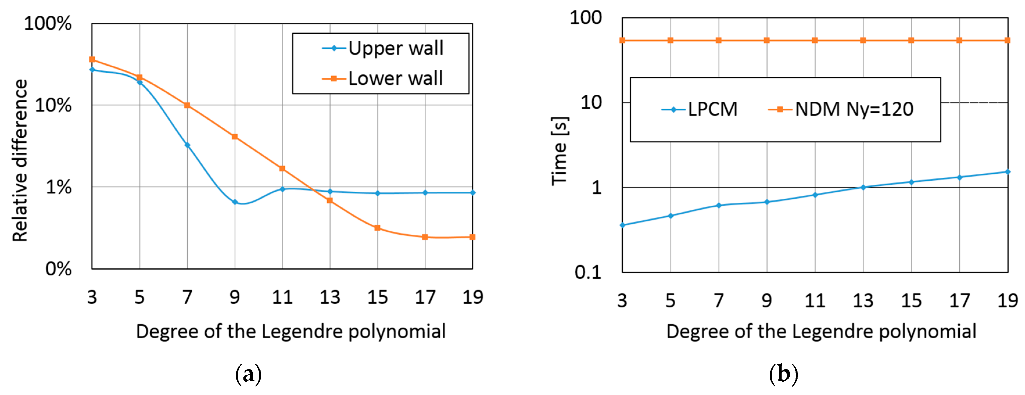
The LPCM results obtained with different numbers of Lobatto points were compared with the reference NDM solution. In
Figure 21a, the relative difference drops rapidly and remains below 1%, starting with 13 Lobatto points.
Figure 21b shows that the computational time for the LPCM does not exceed 2 s, while the reference method takes about 54 s.
6. Example of a Two-Lobe Journal Bearing
The coupled Reynolds and energy equations represent a solver for thermo-hydrodynamic problems in lubricated journal and thrust bearings. However, pure validations are more difficult in the context of lubricated bearings because of the additional effects, such as the film rupture and reformation (cavitation), which must be modeled and dealt with Ref. [
8,
9].
Not the least, several user-defined heat transfer parameters must be specified, and this is mainly done on a trial and error basis. The uncertainties in this kind of problem may therefore be quite important, and comparisons with experimental data are not exactly validations of the numerical approaches.
For the completeness of the present work, the numerical analysis of a real journal bearing is presented in the following. The recent experimental results published by Giraudeau et al. [
10] in 2016 for a two-lobe journal bearing with axial supply grooves were used for comparing numerical predictions with experimental results. The length of the tested bearing was 68.4 mm and its diameter was 100 mm. The radial assembly clearance was 68
, while the radial bearing clearance was 143
. The bearing was lubricated by an ISO VG 46 oil supplied at a constant pressure of 0.17 MPa and a temperature of 43 °C. The following oil characteristics were used for the calculations:
,
, and
. The viscosity of the oil was
at
and
at
. The variation is described by an exponentially decaying law. The angular speed was 3500 rpm and the static load was 6 kN. Only the results for the lower loaded lobe are shown here. Cavitation was dealt with by using the algorithm introduced in Ref. [
11]. This algorithm uses a free boundary formulation of the incompressible Reynolds equation. The problem was then solved with an efficient solver based on the Fischer–Burmeister form, Newton algorithm, and Shur’s complement.
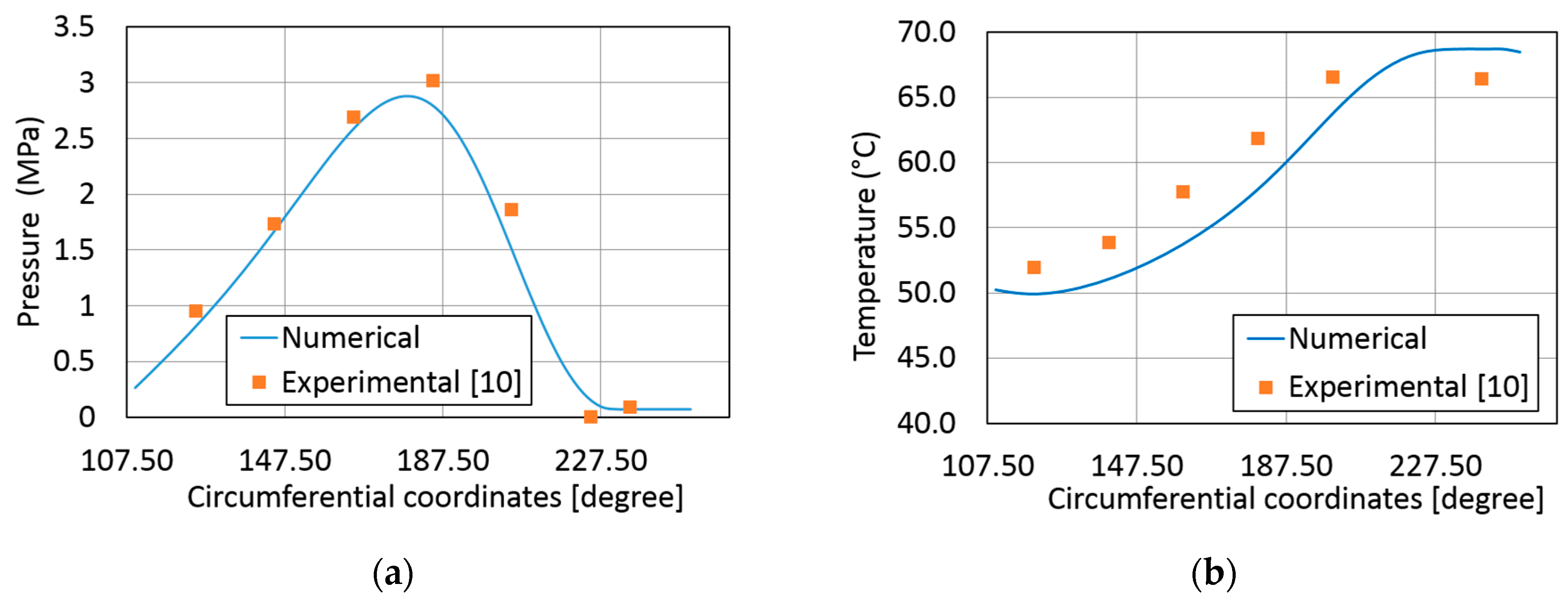
The shaft was considered to have a constant temperature estimated from experiments, while adiabatic wall conditions were imposed on the bushing. The computational domain was discretized using 32 16 cells in circumferential and axial directions, while 11 Lobatto points were used to describe the temperature variation across the fluid film.
Figure 22a,b depicts the pressure and the temperature variations in the circumferential direction of the bearing mid plane. The predicted pressures show good agreement with the measurements, while the predicted temperatures show a reasonable agreement. The quality of the prediction could be improved by including the thermal deformation of the bushing and refining the boundary conditions for the energy equation.
7. Conclusions
The present work focused on the numerical solution of the energy equation in very simple test cases as part of thin fluid films lubrication. The work was motivated by the fact that the complete energy equation has no analytical solution that can be used for comparisons in validations. Therefore, an energy equation decoupled from the Reynolds equation in the case of a 1D slider was imagined, for which the analytical solution of the velocity field was used. The reference values used in all cases presented are detailed in
Appendix B. The second concern was an efficient solver for the energy equation. Two numerical methods were compared: The NDM based on a finite volume discretization, and the LPCM based on a Legendre polynomial approximation of the temperature across the film thickness. The LPCM proved to be one or two orders of magnitude more efficient than the NDM in terms of computation time. This is not negligible if one takes into account that when coupled, the Reynolds and the energy equations are numerically solved in a segregated and iterative manner. The thermo-hydrodynamic calculation of a 1D slider (i.e., for coupled Reynolds and energy equations) confirms this conclusion.
Comparisons of the LPCM thermo-hydrodynamic analyses with the experimental results obtained in a two lobe journal bearing were also presented. However, they are not considered as real validations of the numerical model, since very simple and intuitive boundary conditions of the energy equation were used. Alternatively, the results presented for the 1D slider may be used for validating the first development steps of any solver based on the energy equation for thin film flows.


