Film Thickness and Shape Evaluation in a Cam-Follower Line Contact with Digital Image Processing


1
Dipartimento di Ingegneria Civile e Industriale, University of Pisa, Largo Lazzarino, 56122 Pisa, Italy
2
Direzione Edilizia e Telecomunicazione, University of Pisa, via Fermi 6/8, 56126 Pisa, Italy
3
Parker Hannifin–FCCE, Via Enrico Fermi 5, 20060 Gessate (MI), Italy
*
Author to whom correspondence should be addressed.
Lubricants 2019, 7(4), 29; https://doi.org/10.3390/lubricants7040029
Submission received: 29 January 2019
/
Revised: 15 March 2019
/
Accepted: 25 March 2019
/
Published: 28 March 2019
(This article belongs to the Special Issue Automotive Tribology)
Abstract
:Film thickness is the most important parameter of a lubricated contact. Its evaluation in a cam-follower contact is not easy due to the continuous variations of speed, load and geometry during the camshaft rotation. In this work, experimental apparatus with a system for film thickness and shape estimation using optical interferometry, is described. The basic principles of the interferometric techniques and the color spaces used to describe the color components of the fringes of the interference images are reported. Programs for calibration and image analysis, previously developed for point contacts, have been improved and specifically modified for line contacts. The essential steps of the calibration procedure are illustrated. Some experimental interference images obtained with both Hertzian and elastohydrodynamic lubricated cam-follower line contacts are analyzed. The results show program is capable of being used in very different conditions. The methodology developed seems to be promising for a quasi-automatic analysis of large numbers of interference images recorded during camshaft rotation.

1. Introduction
It is well known that film thickness is one of the most important quantities to be determined for a lubricated contact. Conventionally, engineering methods used for the assessment of film thickness from which a lubrication regime can be determined are often based on numerical and empirical formulations obtained by experimental tests conducted in stationary conditions. However, many practical engineering and mechanical components are characterized by continuous variations of the operating parameters. For instance, non-conformal contacts such as those occurring in gears and cams, are characterized by rapid variations of speed, load and geometry. In these cases, experimental results are difficult to obtain and steady-state numerical solutions can lead to over or underestimation of the film thickness. Although very complex numerical models of the lubricated contacts are available—considering for instance also mixed lubrication conditions, thermal effects and transient conditions—real contacts remain difficult to simulate and experimental studies are therefore important. Only through experimental measurements, in fact, it is possible to obtain a better comprehension of what really happens in the lubricated contacts, providing the possibility of validating numerical models or setting up corrective coefficients for stationary case formulas. During the last decades, the number of experimental investigations on non-steady state lubricated contacts has increased, mainly due to improvements in the experimental techniques and the more sophisticated instrumentation available. In Reference [1] a review of studies on transient conditions is presented. Sample recent studies are reported in References [2,3], in which start-up and sudden halting conditions and the transient behavior of transverse limited micro-grooves in EHL point contacts are investigated. Experimental tests on non-conformal lubricated contacts under transient working conditions are commonly performed using ball on disk test rigs. Often only one quantity is varied, usually the speed of the contacting bodies, while the geometry and the load are kept constant. Few experimental tests have been performed on test rigs for cam-follower contacts. The rapid variation of the operating conditions, typical of the cam-follower contacts, makes it difficult to record the different quantities, particularly those necessary for the evaluation of film thickness. Different methods were used for the measurement of film thickness in cam-follower contacts. A capacitance transducer [4], thin film micro transducers [5] and an electrical resistivity technique [6] were respectively used. Tests on real engines have been also performed, as for instance in Reference [7], where both friction and minimum oil film thickness were measured, the latter with a capacitance technique. However, optical interferometry has proven to be the most powerful and detailed method for measuring film thickness and it is currently a well-established experimental technique [8]. Two different kinds of light can normally be used: white and monochromatic light. Many research groups use these techniques. Some examples are briefly mentioned in the following. In Reference [9] white light interferometry was used with a digital image analysis. A spacer layer was introduced in Reference [10] to allow measurement of very thin film. White light cannot be used for thicknesses greater than about 1 μm; monochromatic light can be used in this case. Luo’s group reported a method based on the relative intensity of images obtained with monochromatic light [11]. This method was further developed by using a multi-beam interference analysis in Reference [12]. In Chen and Huang’s work [13], film thickness was evaluated using monochromatic light. The method is based on an actual intensity–thickness relation curve. Studies using dichromatic or trichromatic light were also performed that use both color and light intensity information. Dichromatic light was used, for instance in References [14,15]. An approach to achieve online measurement of film thickness in a slider-on-disc contact by using dichromatic optical interferometry was reported in the work [16]. Marklund et al. described the intensity base methods with a phase measurement approach using trichromatic light [17]. The combination of conventional chromatic interferometry with the computer image processing methods available nowadays offers good accuracy and the possibility of analyzing a great number of images in an automatic way [18,19] and can also be used to analyze images obtained in line contacts [20].
For the analysis of the large number of images recorded by a high-speed camera, a program for automatic digital image processing was developed for point contacts by the authors’ research group [21]. It was used for the analysis of interference images obtained in tests with constant load and geometry but variable speed using a ball-on-disc experimental apparatus. A test rig was successively designed and realized for a more realistic simulation of gear teeth and cam-follower contacts. The rig was tested using circular eccentric cams [22].
In this work, after a description of the experimental apparatus used, the main issues of the digital image processing of interference images obtained in the line contacts are presented and discussed. The former program, developed for point contact [21], has been improved and new versions for calibration and successive analysis of line contacts have been realized and used for a cylindrical cam in contact with a glass disc.
2. Materials and Methods
2.1. Experimental Test Rig
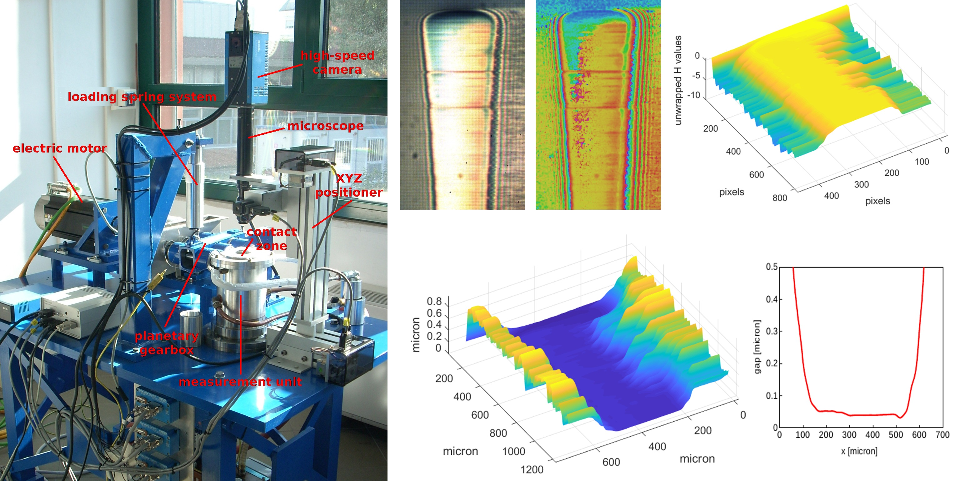
The rig used for the experimental tests, also described in Reference [23], was entirely designed and developed at the University of Pisa in order to investigate non-conformal lubricated contacts between a specimen of suitable shape (usually a cam) and a counterface (usually the flat surface of a disc, simulating a follower). The rig allows simultaneous measurements of contact force and film thickness. A picture and a schematic drawing of the apparatus are shown in Figure 1.
The camshaft is installed on a rocker arm and is driven by a planetary gearbox moved by a brushless electric motor. The rocker arm is connected to the motor by an elastic joint. An absolute encoder positioned after the elastic joint allows the direct measurement of the angular position and velocity of the cam.
The contact between the cam and the plane surface of the disc occurs in the measurement unit. This includes a system of nine annular load cells mounted in three groups, each one composed of two tangential cells and one for normal load. In this way, all components of the contact force are measured. Different configurations are possible by changing the loading system or the measurement group. In the basic version the glass disc, simulating the follower, is kept fixed while the cam axis is moving. The load is applied through an adjustable spring system. Another approach is to apply the load with weights via a lever mechanism mounted on the rocker arm on the opposite side of the spring; this configuration allows better regulation of the contact force, especially during the calibration procedure.
The lubricant is directly supplied to the contact zone by an oil system. The temperature is regulated using a thermostatic bath. Figure 2 shows the cam used for obtaining the results presented in this work mounted on the camshaft; the upper part of the measurement unit with the follower is removed in this picture to make the cam visible.
The test rig is instrumented and controlled using real-time National Instruments cRIO and LabVIEW® software. A sampling frequency of 10 kHz is normally used during tests.
Film thickness and its shape are estimated using optical interferometry. In this case, the disc used for the experiments is made of glass coated with a thin semi-reflective layer of chromium, Cr, and a layer of silicon dioxide, SiO2, to protect the surface from abrasion and to increase the range of thicknesses measurable.
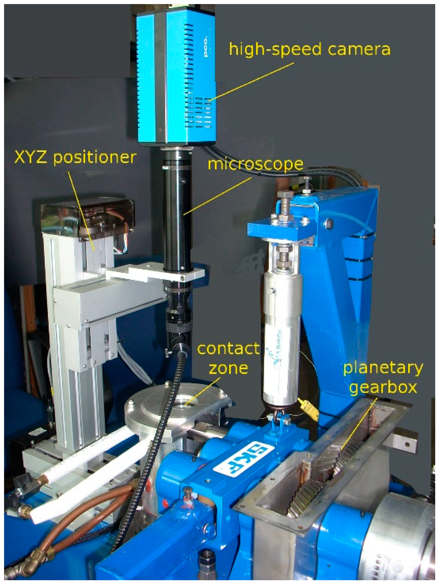
Interference images are recorded by means of a microscope connected to, and moved via, a computer controlled XYZ positioner with an independent step motor for moving each axis. Detail of the test rig with the optical system is shown in Figure 3.
A high-speed camera connected to the microscope allows the recording of interference images with a frame rate of up to 1000 images per second for film thickness measurements also under transient conditions. The images are recorded in the 4 GB camera internal memory and transferred to the computer successively.
The methodology used for obtaining the film thickness and shape is described in detail below.
2.2. Film Thickness Measurement Procedures
It is known that a peculiarity of a cam-follower system is the movement of the contact zone during the rotation of the camshaft. Even using the computer controlled XYZ positioner, depending on the rotational speed and on the cam’s shape, it is not easy to synchronize the target area of the microscope with the contact zone. This is due to the high velocities and accelerations that the contact area can reach and also due to possible vibration problems. Thus, the recording of the interference images along the contact was often achieved by repeating tests in the same working conditions, adopting different positions of the microscope. Images of the contact zone were also obtained by reducing the microscope magnification but the limitation is that the used magnification must be sufficient to distinguish the interference fringes. More details of these aspects are reported in Reference [24].
Once the interference images are recorded, film thickness and shape can be evaluated by a proper elaboration. The methodology developed and used for the elaboration of line contact images is described below. For the sake of completeness, the fundamental aspects of optical interferometry and the color spaces are reported before describing the procedure used.
2.2.1. Fundamentals of Optical Interferometry
As mentioned in the introduction, optical interferometry is a well-known powerful technique for the estimation of the shape and thickness of non-conformal lubricated contacts, developed in the 1960s [25]. This technique is particularly efficient under transient conditions, for which the use of other methods such as capacitance or electrical resistivity is not strictly suggested. Optical interferometry is typically used in ball-on-disc test rigs, but it can be applied to contacts between bodies of different shapes (as a cylindrical cam) and a transparent surface (usually the plane surface of a disc). It is generally based on the interference pattern created by the light beam reflected by a semi-reflecting chromium layer applied to the surface of the disc and the portion of the light beam passing through the fluid, if present, and reflected by the body. Sometimes the glass disc can be coated, on the side of the contact, with a further layer of silicon dioxide to protect the surface from abrasion and also to increase the measurement range towards lower thicknesses. The two beams cover different distances and a phase shift between the two light waves occurs. The interference of the two beams produces greater visibility when the intensity of the two reflected beams is similar. Since the investigation is usually limited to the contact region, the angle formed by the incoming and the reflected beams is very little and practically negligible. The resulting wave will have an amplitude ranging from zero to twice the amplitude of the original wave, that is, destructive and constructive interference, in reference to the phase difference between the two waves. Thus, the interference pattern, consisting of bright and dark fringes, will be visible when monochromatic light is used. The interference pattern results, in white light, in a graduation of colors due to the delay of the beams, which is related to the film thickness. In Figure 4 the basic principle of the optical interferometry technique for fluid film measurement is shown.
The interference light intensity I given by the interference of two beams, with intensities I1 and I2 respectively, can be approximately related to the optical film thickness hopt with the following Equation (1), taking into account the refractive indices ni of the traversed media of thickness hi and the phase difference ϕ caused by the reflection [26]:
being ca the attenuating coefficient of light intensity with the increase of the film thickness due to the low-coherent nature of light, λ0 the wavelength of the spectral light and hopt given by:
Monochromatic or white light can be used. Monochromatic light is characterized by a very narrow spectrum around the wavelength λ0 which, as seen, the measurement of the film thickness is dependent on. In this case, destructive and constructive interference of the beams produces only dark and bright fringes. With white light the changes in phase are revealed by a color transition, for example, from yellow to red or blue to green and so forth. The interferometric image obtained with white light is therefore characterized by a graduation of colored fringes, each one corresponding to a value of the film thickness. These fringes are generated by the interference of beams with different wavelengths λ and refractive index n, therefore the mathematical description of the phenomenon is more complicated if compared with that of monochromatic light. The relationship between film thickness and the colors of the fringes is typically non-linear, thus a calibration table must first be obtained. White light allows greater resolution, commonly a few nm, but it might be limited by the human capacity to distinguish each color, which depends on color vision accuracy. To this purpose, automatic algorithms have been developed. Anyhow, optical interferometry with white light also presents some disadvantages concerned with the limits of the range of measurement when only the semi-reflecting chromium layer is used: a film thickness lower than 0.1 μm leads to a dark zone tending to black (which would mean a thickness equal to zero) and values bigger than 1 μm, due to the low consistency of the light, leads to a vanishing of the fringes. The spacer layer of SiO2 on the glass disc is in fact used to reduce the lower limit (and the upper), shifting downward the range of measurement to the typical values of film thickness of EHL contacts.
For monochromatic light tests, interference filters are often used for filtering the white light to select just the desired wavelength. This leads to a reduction of intensity and so, compared to the images captured using not filtered white light, longer exposure times are needed. Although it does not represent a big issue for steady state experiments, the longer time needed to capture each image might counteract the frame rate of the camera used for transient conditions—for cams typically in the order of milliseconds. Therefore, digital processing of interferometric images obtained with white light has been performed in this work.
2.2.2. Color Spaces in Optical Interferometry
Digital image processing was historically based on RGB (Red, Green, Blue) color space. Another way to represent any chromaticity is the HSV (Hue, Saturation, Value) color space. Some details of the two color spaces and their relationships are reported in Appendix A.
Either RGB or HSV color spaces can be used to analyze interferograms for EHL film thickness measurements since they represent different ways to describe the same information. In the interferometric images obtained with white light, the changes in phase lead to a color transition between fringes of the same hue. Adopting Equation (1) for the resulting interference light along the contact region, each RGB component reveals theoretically sinusoidal behavior with different phases and frequencies. In this case, the calibration process requires particular attention since all three color components must be taken into account. In addition, it is worth remarking that, when RGB deconstruction is applied to interferograms for EHL film thickness measurements, a strong sensitivity to the method used to illuminate the contact area is revealed. In particular, if the light is not uniform, as frequently happens, the RGB components could show different values even if related to the extent that the contact region has the same nominal film thickness. In order to overcome these kinds of difficulties, HSV color space was adopted by the authors. The variation of the H component is similar to an almost periodical signal ranging from 0 to 1, which is able to describe the resulting interference light without any sensitivity in respect to saturation and brightness. It means that, in order to evaluate the film thickness, the digital process of the image can be carried out adopting only the H component of the fringes overcoming in this way all the problems related to the illumination conditions of the contact area. Besides the greater insensibility to the shade and brightness of the light and the illumination conditions, the adoption of the HSV color space also leads to a simplification of the image processing and calibration procedures since only the H component must be analyzed instead of three as is the case for RGB space. In Figure 5a,b sample theoretical distributions of RGB intensities and their correspondent HSV values as a function of optical thickness are given. They have been obtained using Equations (1) and (2) in a simple purposely developed program for the three wavelength for R, G and B and using values similar to those reported in Reference [26]. H, S and V values have been evaluated according to the conversion methods mentioned in Appendix A.
The interference images obtained experimentally do not actually produce regular trends due to some shape irregularities such as surface roughness. In Figure 6b,c an example of RGB and HSV components obtained along the x-axis indicated in the interference image of Figure 6a are shown. The interferogram refers to the line contact occurring between a glass disc and the basic circle of a steel cam having a curvature radius of 14 mm, an axial width of 8 mm and an average value of the root mean square roughness Rq of 0.02 μm. A glass disc without the SiO2 spacer layer was used, as evident from the dark zone corresponding to the Hertzian contact zone. The cam was loaded against the disc using a load of 30 N, producing a Hertzian contact width and pressure equal to 66 µm and 73 MPa respectively. The image, having a size of 350 × 350 pixels, was captured adopting a magnification leading to a pixel length of 1.32 µm. Note that the image is just a portion of the cam contact zone; even using the lower optical magnification, it was not possible to make the entire width of the cam visible in a single image.
As expected, the variation of the H component, at least in the region close to the contact area, assumes an almost periodical behavior. The values of S and V components have an irregular behavior. They do not provide useful information about the changes in film thickness and are not used for the evaluation of the distance between the two bodies in contact.
2.2.3. Elaboration of the Hue Signal
The trend of H is similar to a periodical signal often referred to as “wrapped” hue [21]. By using an algorithm that adds or subtracts an integer to all values subsequent to a discontinuity, a continuous signal—usually called “unwrapped” hue—is reconstructed. The methodology is described in detail in Reference [21] for circular point contacts. The mathematical processing of the wrapped hue values may lead to an amount of noise and uncertainty in the measurement, as shown in Figure 7 where an example of conversion from H to the unwrapped signal, uwH, referred to the processing of the interference image shown in Figure 6a, is shown.
2.2.4. The Image Processing Program
The image processing program developed in Matlab® had already demonstrated its consistency for circular point contacts [21]. In this case, the algorithm did not operate directly on the original wrapped phase map but along a sequence of radial lines at intervals of a predefined angular increment starting from the center of the contact. In this way, the unwrapping procedure is performed by a simple mono-dimensional algorithm that unwraps the signal on each line, deciding to add or subtract integer values by comparing the differences between consecutive elements to a threshold value T < 1. This pseudo-two-dimensional algorithm works properly if the threshold value is set to be no less than twice the maximum noise. Finally, the resulting unwrapped matrix is transformed back into the original coordinates.
In order to achieve the correlation between the fringes and the film thickness, the interference images are then used as input for the image process algorithm in addition to the gap values and pixel length. The program is able to convert the interference pattern in the HSV color space allowing operation on the single H component. The conversion from the wrapped to the unwrapped H signal is dependent on the threshold value T, which can be modified by the user in order to obtain, as much as possible, a monotonic progression of the unwrapped signal along the contact region. At the end of the unwrapping procedure, the user can finally choose, among the matrix of the results obtained for each patterns, which rows must be considered for the calibration and which rows have to be neglected in order to consider only the progressions with a monotonic behavior of the signal; in this way, it is possible to avoid the calibration being affected by scratches on the glass disc or spots on the optical instrumentation. The mean values of the chosen unwrapped signals are put in relation to the theoretical gap between the specimen and the disc in order to obtain the calibration curve, which allows the relation of the H components to the film thickness.
An improvement of the mathematical processing of the wrapped hue has been implemented in order to extend the automatic calibration procedure to the line contact. The same algorithm is used to operate the analysis of line contact images along a sequence of parallel lines instead of radial ones. The distance between two consecutive lines is given by the operator as a number of pixels (one single pixel can also be chosen). The operator also chooses a central zone of the contact from which the lines are swept alternatively to the right and to the left. The program has also been particularly optimized by making some procedures automatic: input data, such as working conditions, pixel length, optical magnification and refractive index can be automatically loaded allowing faster analyses of a large number of images commonly recorded during tests.
3. Results
3.1. Calibration
In order to obtain an evaluation of the film thickness starting from the interferograms, a calibration procedure must first be carried out to relate the H component to the distance between the two bodies in contact. The purpose of image calibration is to find scale and offset factors that can be used to relate the interferometric fringes with the clearance gap between the two bodies. At the end of the procedure, a calibration table containing for each intensity color the corresponding film thickness is obtained.
The calibration of the interferometric images is usually performed by comparing the clearance gap and contact area given by the interferograms analysis with the analogous known values given by theoretical models of contact mechanics. Practically, the most common way to proceed is to capture the image of a Hertzian contact and to then correlate the H value of each point of the interference image with the theoretical gap given by a formula. Different formulas are available for point and for line contacts as reported for instance in Reference [27,28]. A transparent grid is normally used to evaluate the length of each image pixel so that the number of pixels can be converted into distance.
In Figure 9 the color calibration curve obtained with the steel cam loaded against the glass disc is shown; the corresponding colors of the H values are given in the color bar.
3.2. Sample Result for a Hertzian Contact
In order to highlight the efficiency of the developed algorithm, interferometric images obtained with static contacts between the cam base circle and the disc were first analyzed. The calibration curves presented above have been used for the assessment of the distance between the two bodies.
In Figure 10, an example of the application of the procedure described above in the case of a static contact with a load of 30 N in the presence of lubricant is reported.
The interferogram of Figure 10a, with a size of 213 × 563 pixels, was captured with a microscope magnification leading to a pixel length of 1.55 μm. The related 3D unwrapped signal (Figure 10c) has been obtained using 0.1 as a threshold value. The unwrapping procedure has been performed on a sequence of lines crossing the interferometric fringes in order to obtain the gap distribution through the contact region. Figure 10d,e show the 3D representation and the contour lines of the body distance distribution obtained by a successive processing, while a comparison between theoretical and evaluated contact profile along the x-axis in Figure 10e is shown in Figure 10f.
3.3. Sample Results for EHL Contacts
In order to give an idea of the different images that can be elaborated by the program, some images recorded at some particular points during the rotation of the same cam used for the calibration, shown in Figure 11a, have been selected. A synthetic motor oil SAE 5W-40 was used as a lubricant (viscosity and pressure-viscosity coefficient 0.145 Pas and 2.2 × 10⁻⁸ Pa−1 respectively at the test temperature of 26.7 °C). The images reported in the following refer to a test with the cam rotating at 60 rpm contacting the follower with a preload of 30 N (produced by a spring when the contact occurs on the base circle). Due to the not high rotational speed, the trend of the normal force is similar to that of the lift (vertical displacement) shown in Figure 11b, with a maximum value of about 250 N in correspondence with the cam’s nose (position corresponding to 0° in the diagram; the abscissa starts from the point on the base circle opposite to the cam nose). Note that, as reported in Reference [24], the horizontal displacement of the contact point corresponds with the vertical velocity divided by the rotational speed.
The contact positions at −49°, 0° and 125° of rotation angle, indicated by the black circles in Figure 11b, have been selected in order to test the capabilities of the program in very different conditions. Also, different dimensions of the interference images have been chosen. The images were recorded with a frame rate of 500 frames/s.
The interference image shown in Figure 12a (683 × 1147 μm) was recorded at the inversion of the contact motion on rising flank (rotation angle = −49°). The oil inlet is on the left of the image. The normal load was 165 N, the entraining velocity 47 mm/s and the curvature radius 17.6 mm. The enhanced image and the related 3D unwrapped signals are also shown. The 3D representation of the film thickness and the contour lines are shown in Figure 12d,e while the film thickness along the x-axis reported in Figure 12e is shown in Figure 12f.
Note that the image refers to the zone close to the extremity of the cam where some contacts between the two bodies seem to be present. In addition, the central part of the lubricated contact is not perfectly rectangular, showing a certain tapering that can be related to an imperfect parallelism of the two surfaces. However, the typical EHL restriction at the exit appears in the diagrams of Figure 12f.
In Figure 13 the cam nose being in contact with the follower (rotation angle = 0°) is shown. The normal load was 250 N, the entraining velocity 38 mm/s and the curvature radius was 6.3 mm. The interference image of Figure 13a refers again to the zone close to the cam’s extremity. The bigger load and lower velocity together with the slope of the cam produce very low values of the film thickness captured by the elaboration, as shown in the 3D diagram of Figure 13b (note the different full scale of the vertical axis compared to that of Figure 12d).
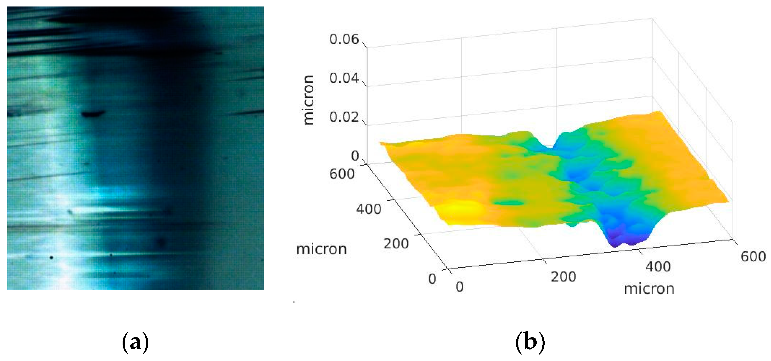
An interference image (294 × 318 pixels) recorded when the contact was on the basic circle (rotation angle = 125°) is shown in Figure 14a. The normal load was 30 N, the entraining velocity 44 mm/s and the curvature radius 14 mm. The interferogram refers to the central part of the contact with dimensions 294 × 318 μm.
4. Discussion
The results presented above show that the program developed for the line contacts between cam and follower is able to analyze very different images recorded during the revolution of the cam. However, there are some aspects related to the peculiarities of the cam-follower contacts that make the analyses difficult and can explain some irregularities in the diagrams shown in the above figures.
The presence of machining marks (see for instance Figure 12a) and surface defects as well as the presence of cavitation zones can create some difficulties for the image analysis. Shape errors and roughness can significantly influence the local values of the film thickness. These defects can also explain the differences between the theoretical and experimental Hertzian profiles shown in Figure 10f.
The not perfect parallelism between the cam and the follower can create a zone in which the film thickness is not sufficient to separate the bodies (local contacts, mixed or even boundary lubrication conditions), as shown in Figure 13. Under these conditions some wear can occur (some scratches are visible in Figure 13a). On the other hand, zones with a film thickness greater than expected can be present on the opposite part of the contact.
Contact conditions vary very quickly at certain angular positions of the cam, for instance when close to the inversion point (−49°). The contact point moves very quickly after the inversion while the entraining velocity is close to zero at −45°. The situation at this point is shown in Figure 15. Note that the film thickness is low but not zero, apart from at the border of the cam (image top), due to some inclination and squeeze effect. The contact point is also moving quickly close to the cam nose (Figure 13). In these conditions a sufficiently high frame rate is important, as it is related to the pixel definition and also to avoid blurry effects. For the present tests, the recording frame rate was limited to 500 frames/s in order to have enough time to store the images corresponding to some cam revolutions in the internal memory of the camera. However higher frame rates could be used with the drawback that a reduced number of cam revolutions would be recorded.
The definition of a single value for the minimum or for the central film thickness—the commonly investigated quantities of a lubricated contact—is not a simple matter for contacts like those investigated. These quantities can vary sometimes in a significant way along the contact (the vertical direction in the images reported in this work). Some investigations could be carried out, averaging methods of the film thickness values obtained along the y direction for each x position.
These aspects deserve specific further investigation.
5. Conclusions and Future Developments
The optical system of a test rig for investigations of cam-follower contacts allows the recording of interference images that are used for the evaluation of film thickness and shape. A description of the interferometric technique and the digital image process used to obtain the 3D profile starting from the recorded images is presented. The color space used to describe the color components of the fringes, and the methodology and procedures and the essential steps necessary to set up the numerical algorithm, are discussed. Numerical programs developed in Matlab® for the analysis of interferometric images that are able to reproduce the three-dimensional profile of line contacts are developed starting with previous versions developed for point contacts. The programs are first used for the digital image process of the wrapped color components for the calibration procedure. The fluid film thickness is assessed by means of the calibration table given adopting the unwrapping procedure.
Some presented results evidence the capabilities of the programs developed and, at the same time, some practical problems intrinsically related to the cam-follower contacts as the quick motion of the contact point, the geometrical errors and the surface defects and the not perfect parallelism of the contacting bodies. However, the methodology developed seems able to perform the analysis of very different images by catching the values of the film thickness during the camshaft rotation.
Several aspects need to be specifically addressed in future investigations. Tests with cams with different geometrical precision will provide more indications of the influence of this factor on the measurements. The possible influence of the frame rate on the images and the corresponding film thickness can be investigated, recording the images with different frame rates. Finally, investigations at different loads, rotational speeds and with different lubricants will be planned to investigate their effects on the evolution of the film shape during rotation.
Author Contributions
Conceptualization, all authors; methodology, all authors; software, G.P. and F.F.; validation, G.P.; formal analysis, all authors; investigation, G.P. and F.F.; resources, E.C.; data curation, G.P. and F.F.; writing—original draft preparation, E.C. and G.P.; writing—review and editing, all authors.
Funding
This research received no external funding.
Acknowledgments
The authors would to thank to Eng. Alessio Lazzaretti and Eng. Giacomo Bassi for their contribution to the experimental work.
Conflicts of Interest
The authors declare no conflict of interest.
Appendix A
RGB color space represents any chromaticity as the results of the components of Red, Green and Blue. In a 3D Cartesian coordinate system, it can be represented by a cube with the three color components as axes (see Figure A1). In this system any point is identified by a combination of three integer values from 0 to 255. Thus, each chromaticity will be expressed as a tern of values (e.g., [255,0,0] for red, etc.) spacing from [0,0,0] to [255,255,255] corresponding to black and white respectively. For a digital image process, 8 bits for each component are needed.
Figure A1.
Conversion RGB cube to HSV hexcone color space.
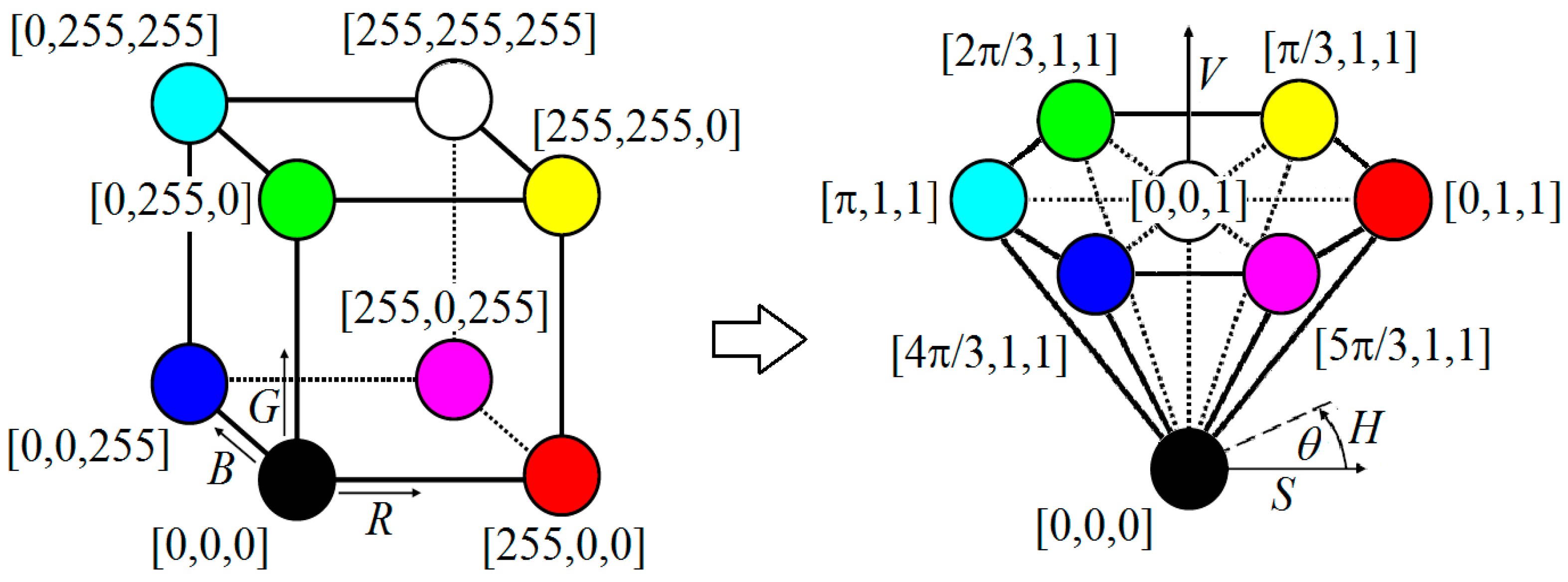
Another way to represent any chromaticity is the HSV space which describes each color (Hue) in terms of shade (Saturation) and brightness (Value). The hue of a color refers to which pure color it resembles (e.g., all tints, tones and shades of red have the same hue); it is expressed by a fraction from 0 to 2π representing the position of the corresponding pure color on the color wheel (e.g., value 0 corresponds to red; π/3 to yellow; 2π/3 to green; etc.). The saturation of a chromaticity describes how white the color is (e.g., a pure red is fully saturated, with a saturation of 1, tints of red have saturations less than 1 and white has a saturation of 0). Finally, the value is related to the brightness, which describes how dark the chromaticity is; V is expressed by a fraction from 0 to 1 corresponding to black and white, respectively. In a 3D Cartesian coordinate system, the HSV color space can be represented by a hexcone having the vertical axis corresponding to the brightness (see Figure A1). The angle around the vertical axis gives the hue with red at θ equal to 0. The saturation is given by a ratio, ranging from zero, on the vertical axis, to one on the sides of the hexcone.
The conversion between RGB and HSV color space components can be obtained through a non-linear, bijective relation which is illustrated in Figure A1 and given by the formulas reported in Reference [29]. Particularly for hue the following equation can be used:
where arctan2 is the four-quadrant inverse tangent. Unfortunately, this relation, which requires a case differentiation depending on the quadrant of the argument, might lead to some difficulties in the mathematical modeling performed by numerical programs, such as the computing language Matlab®. Thus, for the conversion from RGB to HSV the following formulation suggested in Reference [30] was chosen and efficiently tested by the authors:
being
The maximum and minimum values of H are then chosen in order to obtain the red for θ equal to 0 and 2π. For the aim of this work, the HSV components were normalized and ranged between zero and one [31].
References
- Ciulli, E. Non-steady state non-conformal contacts: Friction and film thickness studies. Meccanica 2009, 44, 409–425. [Google Scholar] [CrossRef]
- Myant, C.; Fowell, M.; Cann, P. The effect of transient motion on isoviscous-EHL films in compliant, point, contacts. Tribol. Int. 2014, 72, 98–107. [Google Scholar] [CrossRef]
- Ali, F.; Kaneta, M.; Křupka, I.; Hartl, M. Experimental and numerical investigation on the behavior of transverse limited micro-grooves in EHL point contacts. Tribol. Int. 2015, 84, 81–89. [Google Scholar] [CrossRef]
- Hamilton, G.M. The hydrodynamic of a cam follower. Tribol. Int. 1980, 13, 113–119. [Google Scholar] [CrossRef]
- van Leeuwen, H.; Meijer, H.; Schouten, M. Elastohydrodynamic film thickness and temperature measurements in dynamically loaded concentrated contacts: Eccentric cam–flat follower. In 13th Leeds–Lyon Symposium; Elsevier: Amsterdam, the Netherlands, 1987; pp. 611–625. [Google Scholar]
- Dowson, D.; Harrison, P.; Taylor, C.M.; Zhu, G. Experimental observation of lubricant film state between a cam and bucket follower using the electrical resistivity technique. In Proceedings of the Japan International Tribology Conference, Nagoya, Japan, 29 October–1 November 1990; pp. 119–124. [Google Scholar]
- Mufti, R.A. Experimental technique for evaluating valve train performance of a heavy duty diesel engine. Proc. IMECHE 2009, 223, 425–436. [Google Scholar] [CrossRef]
- Ma, L.; Luo, J.B. Thin film lubrication in the past 20 years. Friction 2016, 4, 280–302. [Google Scholar] [CrossRef] [Green Version]
- Gustafsson, L.; Höglund, E.; Marklund, O. Measuring Lubricant Film Thickness with Image Analysis. Proc. Inst. Mech. Eng. J J. Eng. Tribol. 1994, 208, 199–205. [Google Scholar] [CrossRef]
- Cann, P.M.; Spikes, H.A.; Hutchinson, J. The Development of a Spacer Layer Imaging Method (SLIM) for Mapping Elastohydrodynamic Contacts. Tribol. Trans. 1996, 39, 915–921. [Google Scholar] [CrossRef]
- Luo, J.B.; Wen, S.Z.; Huang, P. Thin film lubrication. Part I. Study on the transition between EHL and thin film lubrication using a relative optical interference intensity technique. Wear 1996, 194, 107–115. [Google Scholar] [CrossRef]
- Guo, F.; Wong, P.L. A multi-beam intensity-based approach for lubricant film measurements in non-conformal contacts. Proc. Inst. Mech. Eng. J J. Eng. Tribol. 2002, 216, 281–291. [Google Scholar] [CrossRef]
- Chen, Y.; Huang, P. An Improved Interference Method for Measuring Lubricant Film Thickness Using Monochromatic Light. Tribol. Lett. 2017, 65, 120. [Google Scholar] [CrossRef]
- Kaneta, M.; Kanada, T.; Nishikawa, H. Optical interferometric observations of the effects of a moving dent on point contact EHL. ASME J. Tribol. 1997, 32, 69–79. [Google Scholar]
- Liu, H.C.; Guo, F.; Guo, L.; Wong, P.L. A dichromatic interference intensity modulation approach to measurement of lubricating film thickness. Tribol. Lett. 2015, 58. [Google Scholar] [CrossRef]
- Bai, Q.; Guo, F.; Wong, P.L.; Jiang, P. Online Measurement of Lubricating Film Thickness in Slider-on-Disc Contact Based on Dichromatic Optical Interferometry. Tribol. Lett. 2017, 65. [Google Scholar] [CrossRef]
- Marklund, O.; Gustafsson, L. Interferometry-based measurements of oil-film thickness. Proc. Inst. Mech. Eng. J. Eng. Tribol. 2001, 215, 243–259. [Google Scholar] [CrossRef]
- Hartl, M.; Krupka, I.; Poliscuk, R.; Liska, M. An Automatic System for Real-Time Evaluation of EHD Film Thickness and Shape Based on the Colorimetric Interferometry. Tribol. Trans. 1999, 42, 303–309. [Google Scholar] [CrossRef]
- Hartl, M.; Křupka, I.; Poliščuk, R.; Liška, M.; Molimard, J.; Querry, M.; Vergne, P. Thin Film Colorimetric Interferometry. Tribol. Trans. 2001, 44, 270–276. [Google Scholar] [CrossRef]
- Křupka, I.; Šperka, P.; Hartl, M.; Xue Jin, S.; Yang, C.X. Effect of real longitudinal surface roughness on lubrication film formation within line elastohydrodynamic contact. Tribol. Int. 2010, 43, 2384–2389. [Google Scholar] [CrossRef]
- Ciulli, E.; Draexl, T.; Stadler, K. Film thickness analysis for EHL contacts under steady-state and transient conditions by automatic digital image processing. Adv. Tribol. 2008, 2008, 325187. [Google Scholar] [CrossRef]
- Ciulli, E.; Fazzolari, F.; Piccigallo, B. Experimental study on circular eccentric cam–follower pairs. Proc. Inst. Mech. Eng. J J. Eng. Tribol. 2014, 228, 1088–1098. [Google Scholar] [CrossRef]
- Fazzolari, F.; Ciulli, E.; Vela, D. A novel instrumentation for contact force measurement in cam-follower pairs. In Proceedings of the 18th International Colloquium Tribology, Industrial and Automotive Lubrication, Esslingen, Germany, 10–12 January 2012. [Google Scholar]
- Pugliese, G.; Ciulli, E.; Fazzolari, F. Experimental aspects of a cam-follower contact. In Proceedings of the Accepted for Presentation to the 15th IFToMM World Congress, Krakow, Poland, 30 June–4 July 2019. [Google Scholar]
- Cameron, A.; Gohar, R. Theoretical and experimental studies of the oil film in lubricated point contact. Proc. R. Soc. A 1966, 291, 520–535. [Google Scholar]
- Eguchi, M.; Yamamoto, T. Film thickness measurement using white light spacer interferometry and its calibration by HSV color space. In Proceedings of the 5th International Conference on Tribology, Parma, Italy, 20–22 September 2006; pp. 20–22. [Google Scholar]
- Cameron, A. The Principles of Lubrication; Wiley: New York, NY, USA, 1966. [Google Scholar]
- Johnson, K.L. Contact Mechanics; Cambridge University Press: Cambridge, UK, 1985. [Google Scholar]
- Marklund, O. Interferometric Measurements and Analysis with Applications in Elastohydrodynamic Experiments. Ph.D. Thesis, Lulea University of Technology, Luleå, Sweden, 1998. [Google Scholar]
- Gonzalez, R.C.; Woods, R.E. Digital Image Processing, 3rd ed.; Prentice Hall: Upper Saddle River, NJ, USA, 2008. [Google Scholar]
- Berns, R.S.; Billmeyer, F.W.; Saltzman, M. Billmeyer and Saltzman’s Principles of Color. Technology; Wiley: New York, NY, USA, 2000; pp. 20–32. [Google Scholar]
Figure 1.
(a) Picture of the experimental apparatus for testing cam-follower contacts; (b) Schematic drawing of the apparatus.
Figure 1.
(a) Picture of the experimental apparatus for testing cam-follower contacts; (b) Schematic drawing of the apparatus.

Figure 2.
Picture of the top part of the measurement unit with the cover removed showing the cam mounted on the camshaft and the final part of the oil supply system.
Figure 2.
Picture of the top part of the measurement unit with the cover removed showing the cam mounted on the camshaft and the final part of the oil supply system.
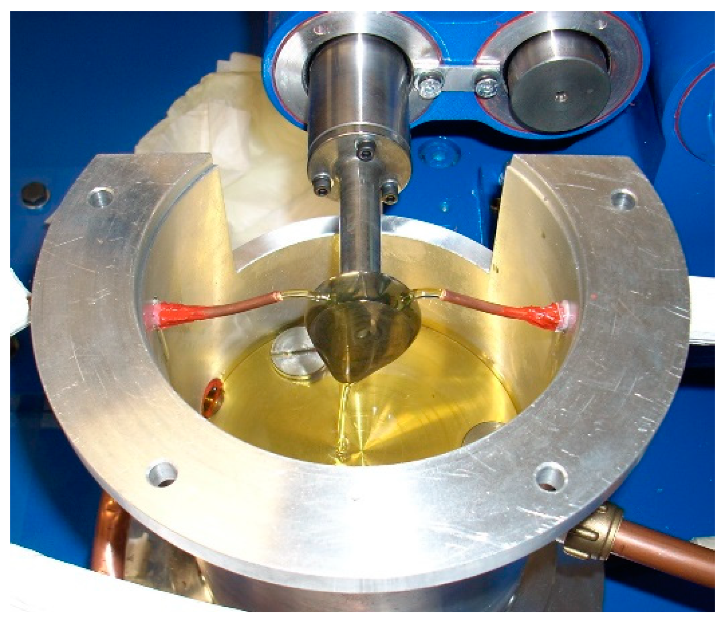
Figure 3.
Picture of the optical system.

Figure 4.
Basic principle of optical interferometry technique.
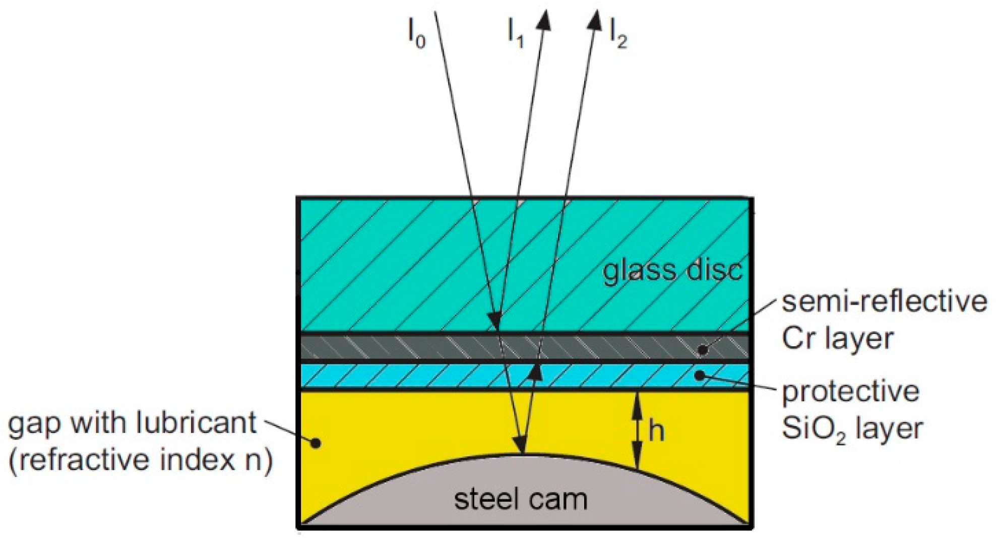
Figure 5.
(a) Theoretical distributions of RGB intensities and (b) corresponding HSV values as function of the optical thickness.
Figure 5.
(a) Theoretical distributions of RGB intensities and (b) corresponding HSV values as function of the optical thickness.

Figure 6.
(a) Interferogram; (b) corresponding RGB and (c) HSV components on x-axis.

Figure 7.
H and unwrapped signals uwH along a pixel row starting from the center of Figure 6a.
Figure 7.
H and unwrapped signals uwH along a pixel row starting from the center of Figure 6a.
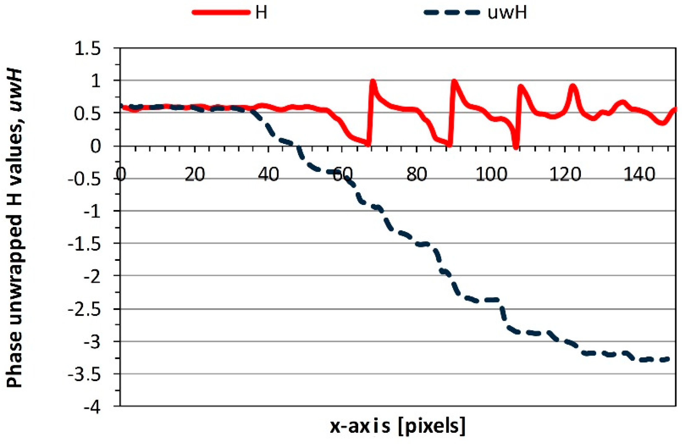
Figure 8.
Block diagram of the program for the elaboration of interference images.
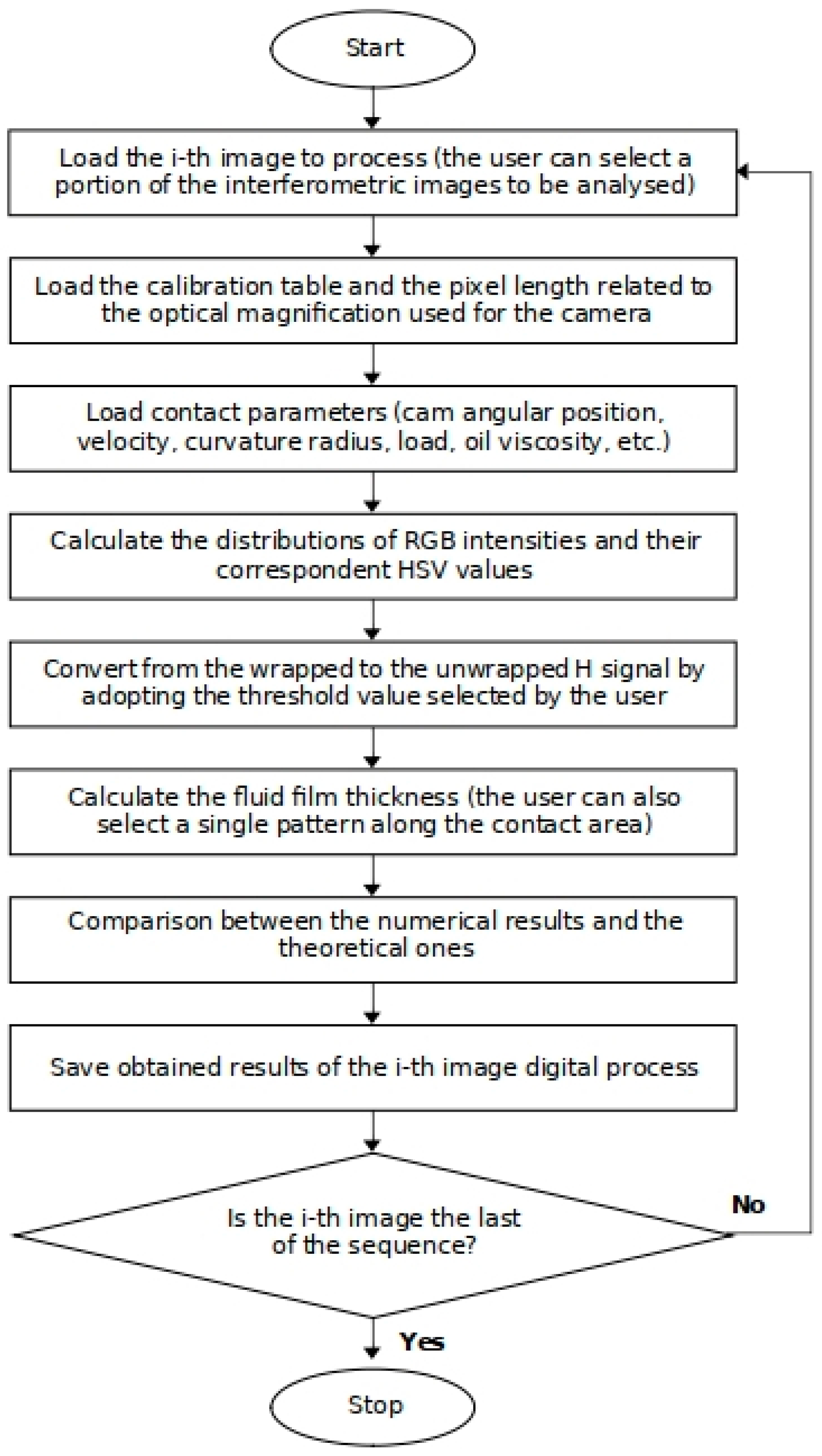
Figure 9.
Calibration table and color bar for cam on glass disc in test basic configuration.

Figure 10.
(a) Interferogram; (b) corresponding enhanced image and (c) related 3D unwrapped signals; (d) 3D representation of the gap; (e) contour lines; (f) comparison between theoretical and evaluated contact profile along the x-axis reported in subfigure (e)—static contact–load 30N.
Figure 10.
(a) Interferogram; (b) corresponding enhanced image and (c) related 3D unwrapped signals; (d) 3D representation of the gap; (e) contour lines; (f) comparison between theoretical and evaluated contact profile along the x-axis reported in subfigure (e)—static contact–load 30N.
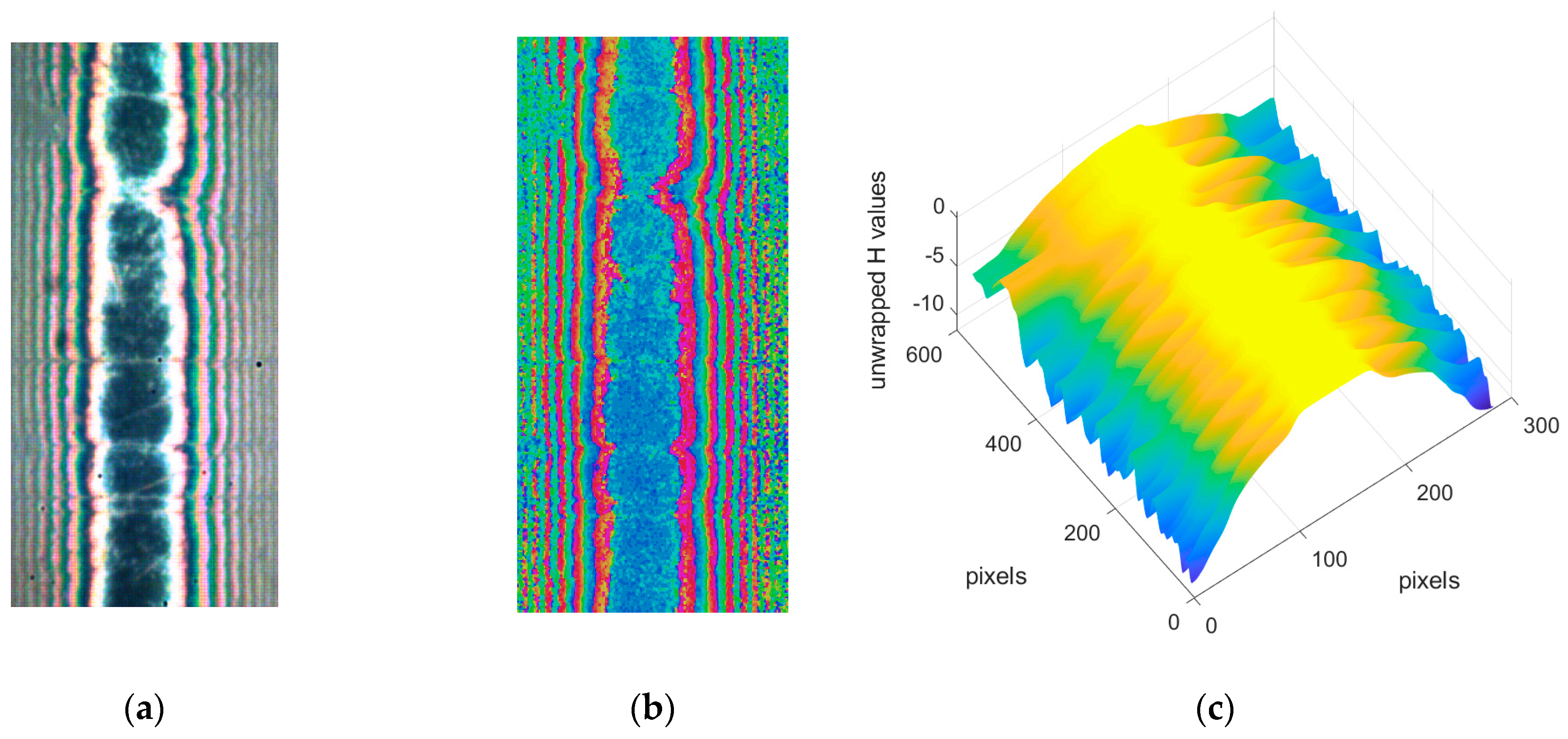
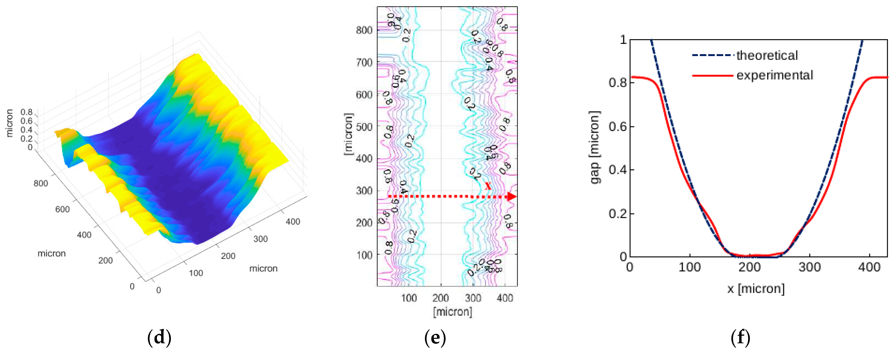
Figure 11.
(a) Cam; (b) vertical and horizontal displacement of the contact zone.

Figure 12.
(a) Interferogram at the inversion point −49°; (b) corresponding enhanced image; (c) related 3D unwrapped signals; (d) 3D representation of the gap; (e) contour lines; (f) film thickness along the x-axis reported in subfigure (e).
Figure 12.
(a) Interferogram at the inversion point −49°; (b) corresponding enhanced image; (c) related 3D unwrapped signals; (d) 3D representation of the gap; (e) contour lines; (f) film thickness along the x-axis reported in subfigure (e).
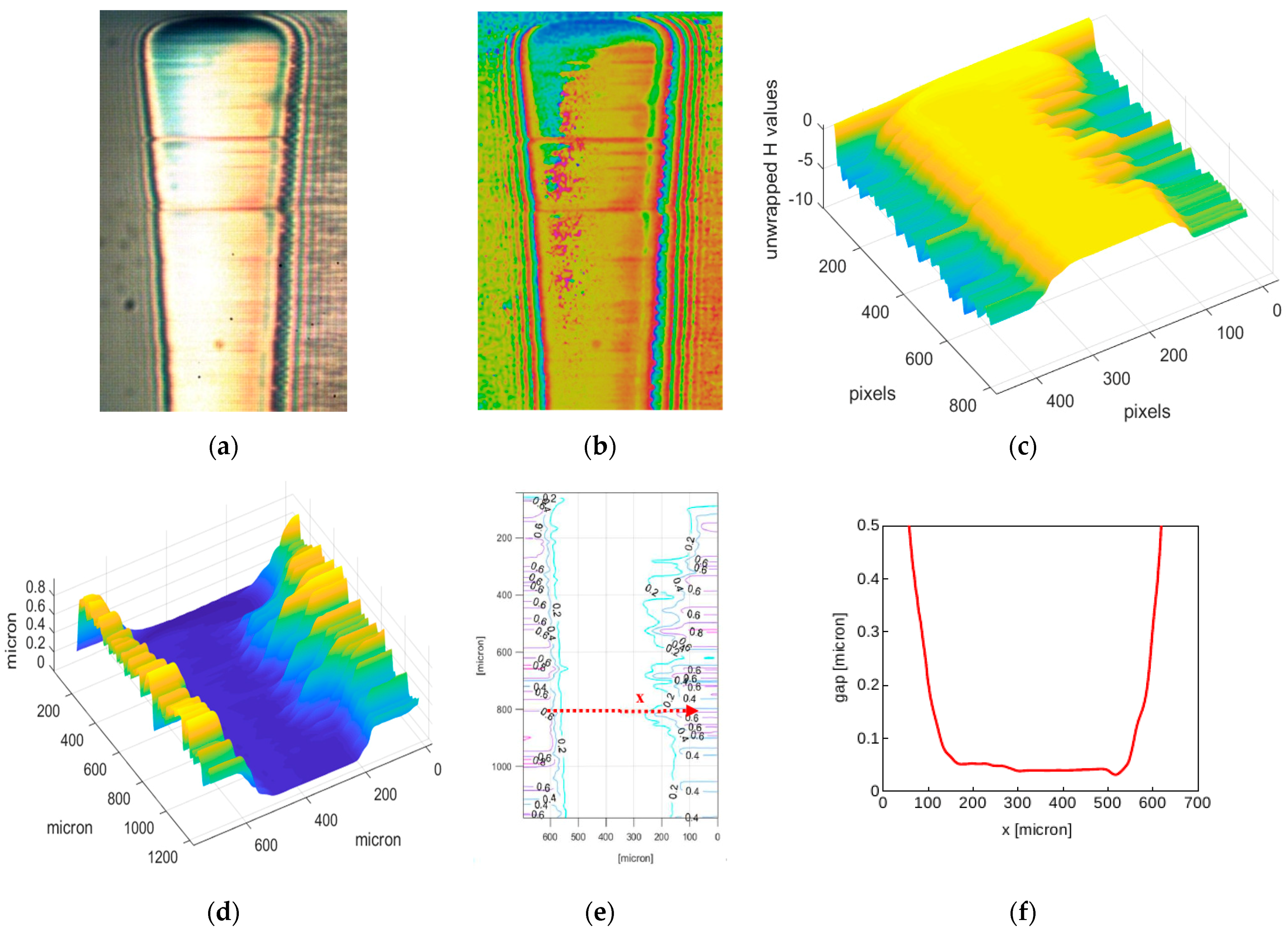
Figure 13.
(a) Interferogram at 0° (cam nose); (b) fluid film 3D representation.

Figure 14.
(a) Interferogram at 125°; (b) fluid film 3D representation; (c) film thickness along the x and y axes shown in subfigure (a).
Figure 14.
(a) Interferogram at 125°; (b) fluid film 3D representation; (c) film thickness along the x and y axes shown in subfigure (a).
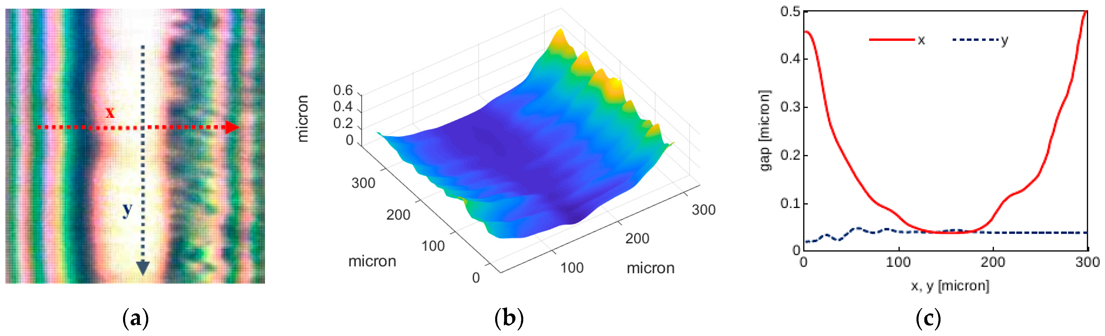
Figure 15.
(a) Interferogram at −45°; (b) fluid film 3D representation; (c) film thickness along the x and y axes shown in subfigure (a).
Figure 15.
(a) Interferogram at −45°; (b) fluid film 3D representation; (c) film thickness along the x and y axes shown in subfigure (a).

© 2019 by the authors. Licensee MDPI, Basel, Switzerland. This article is an open access article distributed under the terms and conditions of the Creative Commons Attribution (CC BY) license (http://creativecommons.org/licenses/by/4.0/).
Share and Cite
MDPI and ACS Style
Ciulli, E.; Pugliese, G.; Fazzolari, F. Film Thickness and Shape Evaluation in a Cam-Follower Line Contact with Digital Image Processing. Lubricants 2019, 7, 29. https://doi.org/10.3390/lubricants7040029
AMA Style
Ciulli E, Pugliese G, Fazzolari F. Film Thickness and Shape Evaluation in a Cam-Follower Line Contact with Digital Image Processing. Lubricants. 2019; 7(4):29. https://doi.org/10.3390/lubricants7040029
Chicago/Turabian StyleCiulli, Enrico, Giovanni Pugliese, and Francesco Fazzolari. 2019. "Film Thickness and Shape Evaluation in a Cam-Follower Line Contact with Digital Image Processing" Lubricants 7, no. 4: 29. https://doi.org/10.3390/lubricants7040029
Note that from the first issue of 2016, this journal uses article numbers instead of page numbers. See further details here.