
Flow Stress Optimization of Inconel 718 Based on a Coupled Simulation of Material-Forming Analysis and Joule Heating Analysis


1
Department of Convergence Engineering, Jungwon University, Goesan-gun 28024, Republic of Korea
2
Research Engineer/R&D Center, FMK, Changwon-si 51395, Republic of Korea
3
Aero-Mechanical Engineering, Jungwon University, Goesan-gun 28024, Republic of Korea
*
Author to whom correspondence should be addressed.
Metals 2022, 12(12), 2024; https://doi.org/10.3390/met12122024
Submission received: 8 October 2022
/
Revised: 28 October 2022
/
Accepted: 21 November 2022
/
Published: 25 November 2022
(This article belongs to the Section Metal Casting, Forming and Heat Treatment)
Abstract
:Inconel 718 is a well-known nickel-based superalloy used for high-temperature applications. The aim of the present study was to formulate a constitutive equation (CE) that can be used to account for the deformation behavior of Inconel 718. Compression tests were performed using Gleeble 3800, a thermomechanical simulator, at temperatures ranging from 900 to 1200 °C, at strain rates varying from 0.1 to 10/s. Before compression tests, each specimen was rapidly heated to the desired test temperature while the initial contact pressure was kept relatively low. Thus, compression was performed while the temperature of the entire system, including the specimen and the die, was not uniform. Before conducting an upsetting finite element analysis to determine CE parameters, the heating conditions applied in the Gleeble tests were first subjected to a Joule heating analysis, to simulate the temperature distribution in each specimen prior to the compression process. The spatial temperature distribution of the specimen and the die were determined using a Joule heating analysis, and these results were used as input data for the subsequent finite element analysis of the compression process. From this, the parameters in the obtained Hansel–Spittel equation were estimated for each temperature condition, by employing the regression optimization method, which was used to minimize the deviation between experimental and simulated load values. To validate this optimization process, the experimentally measured flow stresses with respect to the strain rate for each temperature condition were compared with the forming load, determined by the finite element analysis of the compression process using the optimized CE obtained in the present study. It was confirmed that when the optimization process was applied, there was a decrease in the root mean square error. The major findings confirmed the validity of the CE optimization method combined with Joule heating analysis for determining the CE’s parameters for high-temperature applications.
1. Introduction
Inconel 718 is a super heat-resistant nickel-based alloy designed as a cost-effective alloy, where Co is replaced by about 20% Fe. This innovative material has been widely used in various applications due to its workability and formability. It is superior to other super heat-resistant alloys and has excellent mechanical properties up to 650 °C. Currently, Inconel 718 accounts for 35% of the super heat-resistant alloys used as components in gas turbines, steam turbines, high-temperature industrial power generation equipment, disks for aircraft engines, and oil drilling tubes, which all require high corrosion resistance as well [1]. Demand for Inconel 718 has been increasing with the recent growth of industries with highly corrosive process conditions. However, this material cannot be cold-formed because its room-temperature tensile strength is as high as 1350 MPa. Accordingly, its thermal deformation behavior needs to be studied to allow for high-temperature forming, and to predict and control the occurrence of potential defects.
Materials and alloys subjected to forming processes in industrial fields end up with various temperature, strain, and strain rate histories due to the complex forming methods. Workers who design forming processes must have a clear understanding of the deformation behavior of the metals and alloys to be processed under elevated temperature conditions, to determine the optimal working conditions to ensure their formability and improve their quality.
Constitutive equations (CE) are models used to predict the flow stress of a test material under various forming conditions, including temperature, strain, and strain rate. CEs for elevated temperatures include various equations, such as Arrhenius-type models [2], Johnson–Cook models [3], Hansel–Spittel models [4], Zerilli–Armstrong models [5], and Khan–Huang models [6], and the Arrhenius-type constitutive equation has been widely used for high-temperature flow analyses. Rao et al. [7] performed high-temperature compression tests on carbon steel to determine the desired flow stress for hot forming and confirmed that the developed Arrhenius-type constitutive equation fitted the experimental results well, even though the strain rate changed during deformation. Arrhenius-type constitutive equations have also been widely applied to other materials. For example, Zou et al. [8] and Kang et al. [9] used super-duplex stainless materials 21Cr and S32760 to formulate their high-temperature flow behavior with Arrhenius-type equations. Detrois et al. [10] and Lizzi et al. [11] employed Arrhenius-type equations to predict the high-temperature properties of Inconel materials, especially with respect to their flow behavior.
Conversely, Johnson–Cook models have mainly been applied for the analysis of machining processes. The flow stress of the test material was estimated by performing tensile tests at temperatures ranging from room temperature to 900 °C [12,13,14]. Hansel–Spittel models are mainly used for high-temperature material-forming analysis. Liang et al. [15] measured the displacement–load response of HNi55-7-4-2 alloys using compression tests at elevated temperatures to formulate a Hansel–Spittel constitutive equation. Additionally, the prediction accuracy of the developed constitutive equation could be further improved by applying the friction coefficient of the die as a parameter in the equation. Wang et al. [16] employed a Hansel–Spittel constitutive equation to predict the warm and hot deformation behavior of 20Cr2Ni4A alloys and concluded that the fitness of the equation was improved when the flow stress was used as a parameter in the form of a hyperbolic function.
Recently, regression analysis has been increasingly used to determine equation parameters, as discussed above, to minimize errors between experimental and simulated results. Various attempts have been made to improve the prediction accuracy of Arrhenius-type CEs using regression analysis. For example, Peng et al. [17] and Yin et al. [18] formulated the CE parameters of TC4-DT and GC15 alloys as fifth to sixth polynomials as a function of the strain rate, respectively. It was demonstrated that the average absolute relative error (AARE) could be reduced by adjusting the Zener Holloman parameter.
Ge et al. [19] formulated the CE parameters of Ti-Al alloys as a seventh polynomial and concluded that a correlation coefficient (R) of up to 0.9961 could be achieved. Xu et al. [20] demonstrated that the scope of application of CEs for 20CrMoA alloys could be extended by segmenting the temperature range considering their phase transition behavior in both warm- and hot-forming conditions. Sekar et al. [21] reported that the force prediction in the FE analysis of Ti6Al4V titanium alloys was improved by 3–16% by optimizing the Johnson–Cook CE parameters using the Taguchi method. Niu [22] verified that the regression-optimized CE for Ti-6Al-4V alloy was more accurate in predicting the forming load than the original Hansel–Spittel CE. Chen [23] also confirmed the accuracy of the regression optimization method for X12 ferritic heat-resistant steel. The results were compared with the experimentally measured forming loads using forming tests to determine and compare the prediction accuracy of each equation.
Mirzaire et al. [24] implemented the softening phenomenon of the high-temperature flow of 0.5C-0.68Mn-0.20Si-0.28Cu steel by defining the Z-A model variable as a polynomial equation and introducing peak strain. Mahalle et al. [25] adopted the KHL model formulating the anisotropic deformation CE parameter for the flow stress through the tensile test in the Inconel 718 at the range of room temperature to 700 °C and showed that the thickness and dimensions after deep drawing could be accurately predicted. Piao et al. [26] optimized the parameters of the Lim–Huh model at ultra-high strain rates for the AISI 4340 material and showed that the extrapolated flow stresses of the dynamic hardening models can be precisely calculated.
Recently, comparative and optimization studies using CE and ANN on flow stress are being conducted. Wang [27] and Shang [28] experimentally obtained the deformation information of Ti-6Al-4V alloy and aluminum 5182-O using ABI and tensile tests, respectively, and calculated flow stress using Johnson–Cook, Khan–Huang–Liang-modified Zerilli–Armstrong, and Lim–Huh CE models and the artificial neural network (ANN) method. They concluded that the ANN method was more accurate and efficient than CE models. Li et al. [29] identified the deformation behavior of the DP800 material at the range of room temperature to 300 °C with a large difference in strain rate through iterative finite element analysis using machine learning techniques. In general, flow stress is experimentally determined by performing compression tests under various strain rates and temperature conditions, followed by numerical calculation using the obtained forming load and displacement data. This calculation is performed under the assumption that the strain rate and temperature are uniformly distributed throughout the volume of each specimen. However, Men et al. [30] reported that an increase in the temperature of the specimen used in a Gleeble simulator, which is widely used for high-temperature compression tests, can result from Joule heating and lead to a temperature difference between the specimen and the die. This demonstrated that the applied electric current and resistivity could also serve as process parameters. These results suggest that performing material-forming analysis with the assumption that the temperature of the specimen and the die are uniformly distributed may lead to a temperature difference between the experimental and simulated measurements, thereby causing errors in the determination of flow stress based on optimization simulations.
In the present study, a method for estimating high-temperature flow stress was combined with a Joule heating analysis, where the spatial temperature distribution of not only the specimen but also the die was considered, to improve the prediction accuracy of flow stress models. To this end, the present study proposed a method for estimating the heating condition. In this approach, the temperature measured at a specific point on the specimen is equivalent to that expected for the applied condition at that very point, using a Joule heating analysis of the heating process. The estimated heating condition was then used to calculate the temperature distribution of the specimen and the die prior to the compression test.
The present study examined flow stress, which is considered more effective when simulating the load conditions of compression tests. The optimization of flow stress was then performed by regression analysis of the parameters of a Hansel–Spittel equation. Subsequently, a material-forming analysis was performed based on the optimized flow stress, and the simulated load values before and after optimization were compared with the experimentally measured load values. The accuracy of the flow stress prediction in the Hansen–Spittel equation, considering temperature changes in the specimen and die, was improved by 34.8% after the optimization process.
2. Hot Compression Test
An Inconel 718 billet with a diameter of 30 mm was processed into high-temperature compression test specimens with dimensions of Φ8 × 12 mm. Hot compression tests were performed using a Gleeble 3800 (Dynamic System Inc, New York, USA). The specimens were heated to the deformation temperature (950, 1050, 1150, or 1200 °C) at a rate of 10 °C per second and then held at the temperature for three minutes to ensure a uniform temperature distribution. A thermocouple was attached to the center surface of the specimen at half of its height to measure the heating temperature. The heating cycles for each deformation temperature used in the Gleeble compression tests are presented schematically in Figure 1. A graphite lubricant was applied to the contact surface of each compression test specimen to reduce friction on both sides. The strain rate was set to 0.1/s, 1/s, and 10/s, and all tests were conducted at least twice for each condition.
Load–displacement curves of the compression tests were obtained for the deformation temperature and the applied strain rate, as shown in Figure 2. Assuming that the deformation was uniformly distributed, the true strain and true stress can be calculated based on the experimental load–displacement data using Equations (1) and (2). The relationship between the calculated effective strain and flow stress was plotted with respect to the deformation temperature and strain rate, as shown in Figure 3.
where, ε is the true strain, σ is the true stress or flow stress, is the force, is the surface, and and are the specimen height before and after deformation, respectively.
At strain rates of 0.1/s and 1/s, the true stress remained almost the same as when the true strain was 0.1 or higher. However, when the strain rate was 10/s, the true stress peaked and then started to decrease.
3. Electrical Heating Simulation of Inconel 718
The flow stress calculation using compression test results is normally performed under the assumption that the temperatures of the specimen and die are uniformly distributed. However, in this study, to consider the precise temperature condition of the specimen and die just before upsetting, Joule heating finite element analysis was performed so that the spatial temperature distribution of the specimen and the die could be determined.
The specimen heating process involved Joule heating from the electrical contact resistivity between the specimen and the die and was also accompanied by heat transfer via conduction between the specimen and die, as well as convection with the environment. The governing equation for the Joule heating analysis in the present study was obtained from a previous study on the relationship between electrical and Joule heating [31]. This governing equation can be expressed in a derivative form, as shown in Equation (3). Here, J is the current density (A/m2), and E is the intensity of the electric field. For a material with a conductivity of σ, the relationship: J = σE, holds.
where is the power, is the volume, and is the resistivity. Accordingly, the applied current and the resistivity of the material are input values for the resistive heating analysis. Forge NxT, a software package used in the present study, did not allow the temperature to be controlled by adjusting the resistive heating speed (°C/s). Thus, it was necessary to determine input conditions using the applied current and resistivity to implement the heating cycles described in Figure 3.
The thermal properties of Inconel 718 used for the finite element analysis of heat transfer, including the specific heat capacity, thermal conductivity, density, and electrical resistivity, were used as input data for the analysis of the heating process. These data were from Fan [32] and Jmatpro results. The thermal properties of HD1888 tungsten alloys such as thermal expansion coefficient, thermal conductivity, etc., were referenced from the database of Forge NxT for Joule heating analysis.
Other boundary conditions related to the heat transfer analysis were set: ambient temperature was set to 20 °C, the convection heat transfer coefficient between the material/die and the air was set to 5 W/m2/°C, and the electrical contact resistivity between the material and the die was fixed at Ωm2. By fixing the values of these parameters, Joule heating was controlled using only the electric current in the heat transfer analysis.
To measure the temperature, a thermocouple was attached to the center surface of the specimen at half of its height (1/2H point). To achieve a rate of increase of 10 °C/s, as shown in Figure 3, the applied current had to be appropriately controlled with respect to the heating time and temperature. The amount of current equivalent to that of the applied heating cycle was estimated using iterations and subroutines.
The amount of current required to achieve a heating rate of 10 °C/s was calculated by setting the incremental step of heating duration to one second. The amount of input current in relation to the heating duration, calculated using the subroutines of Forge NxT, is presented in Figure 4. Figure 5 shows the corresponding temperature simulation results.
The simulation results from the Joule heating analysis showed that the temperature approached the target value at the 1/2H point used for the temperature measurement. However, the temperature became lower closer to the interface between the specimen and the die. This meant that accurately estimating the flow stress using regression analysis required analysis of not only the compression process, but also the heating process.
4. Optimization of Parameters in the Hansel–Spittel Equation
The Hansel–Spittel model provided by Forge NxT was used as the CE to optimize the flow stress parameters by upsetting analysis. The relationship between the flow stress, σ, strain rate, , strain, ε, and deformation temperature, T, can be expressed as Equation (4):
By taking the logarithm of both sides of Equation (4), the relationship can be expressed as a polynomial, as shown in Equation (5):
For parameters of the polynomial, only those related to the deformation temperature, strain, and strain rate, i.e., m1, m2, m3, and m4, were retained. The m5 and m8, which were affected by two of the above factors at the same time, and m7 and m9, which were redundant, were excluded. This is to reduce the number of repeated finite element analyses for flow stress optimization.
The modified Hansel–Spittel equation used is presented in Equation (6). In a logarithmic scale, the equation can be expressed as Equation (7):
4.1. Comparison of Experimental and Analysis Results before Flow Stress Optimization
This study aimed to optimize the flow stress of Inconel 718 to reduce errors between the experimental and analysis results. Thus, A, m1, m2, m3, and m4, the parameters that constitute the Hansel–Spittel equation, were optimized, and the high-temperature Gleeble compression test results were compared with the corresponding simulation results.
In an attempt to confirm the validity of this optimization process, the flow stress data obtained from high-temperature Gleeble compression tests, presented in the true stress–true strain curves in Figure 2, were used without optimization in the simulation of the high-temperature Gleeble compression process.
Not only the applied current but also the temperature distribution of the used material and jig, parameters necessary for the simulation of Gleeble compression tests, were calculated using the electrical heating simulation. Finite element analysis of the compression process was performed using the experimentally measured flow stress data points in Figure 2 as input data. The boundary conditions for finite element analysis of Joule heating and upsetting processes used are summarized in Figure 6.
The temperature distribution determined in the finite element analysis of Joule heating was compared with that achieved after upsetting when the deformation temperature was 950 °C and the strain rate was 10/s, as shown in Figure 7. Furthermore, the simulated force determined by analysis of the strain rate with respect to the deformation temperature was compared with the experimentally measured force, as shown in Figure 8.
4.2. Comparison of Experimental and Analysis Results after Flow Stress Optimization
The flow stress of Inconel 718 was calculated by optimizing A, m1, m2, m3, and m4, the five parameters of the modified Hansel–Spittel equation (Equation (6)), using the optimization module provided by Forge NxT 3.2. In this optimization module, the simulation stage for parameter optimization is called a generation. An individual refers to the computation of a given parameter as a specific parameter. Thus, the number of individuals is determined by the number of computations performed. Forge NxT 3.2’s optimization module selects at least two individuals from each generation to perform an analysis based on the design of experiment (DOE) technique.
The displacement–load data obtained from the Gleeble compression tests were used as reference data for the evaluation of optimization results. The calculation results for multiple individuals were then evaluated using the cost function presented in Equation (8), and a new generation (next generation) was accordingly created based on a genetic algorithm:
Parameter optimization was performed using Forge NxT 3.2′s optimization module. For each temperature condition, three strain rates (0.1/s, 1/s, and 10/s), five parameters (A, m1, m2, m3, and m4), and the required time and number of optimization simulations were considered. The number of generations was set to 10, and the number of computations was set to 2. The required number of optimization simulations for each temperature condition was estimated to be 300. Overall, a total of 1200 optimization simulations were performed for the 4 temperature conditions.
Figure 9 shows changes of each parameter as a function of the number of optimization simulations performed. Figure 9a presents changes in the cost function, while Figure 9b–f show changes in each parameter during the optimization simulations. As the cost function decreased, each parameter tended to converge to a certain value. The values of each parameter from the optimization simulations are listed in Table 1. These parameter values were then substituted into the Hansel–Spittel equation to calculate the flow stress, as shown in Figure 10. The flow stress achieved at each temperature was lower than that calculated based on the corresponding experimental data. This was attributed to the non-uniform temperature distribution in the Gleeble specimen, as previously shown in Figure 7. The temperature near the interface with the die was over 70 °C lower than that measured at the point where the thermocouple was attached, which led to an increase in the average flow stress. This phenomenon became more distinct as the deformation temperature increased, as shown in Figure 10a–d, which show the difference between the calculated flow stress based on the experimental data, and the optimized flow stress.
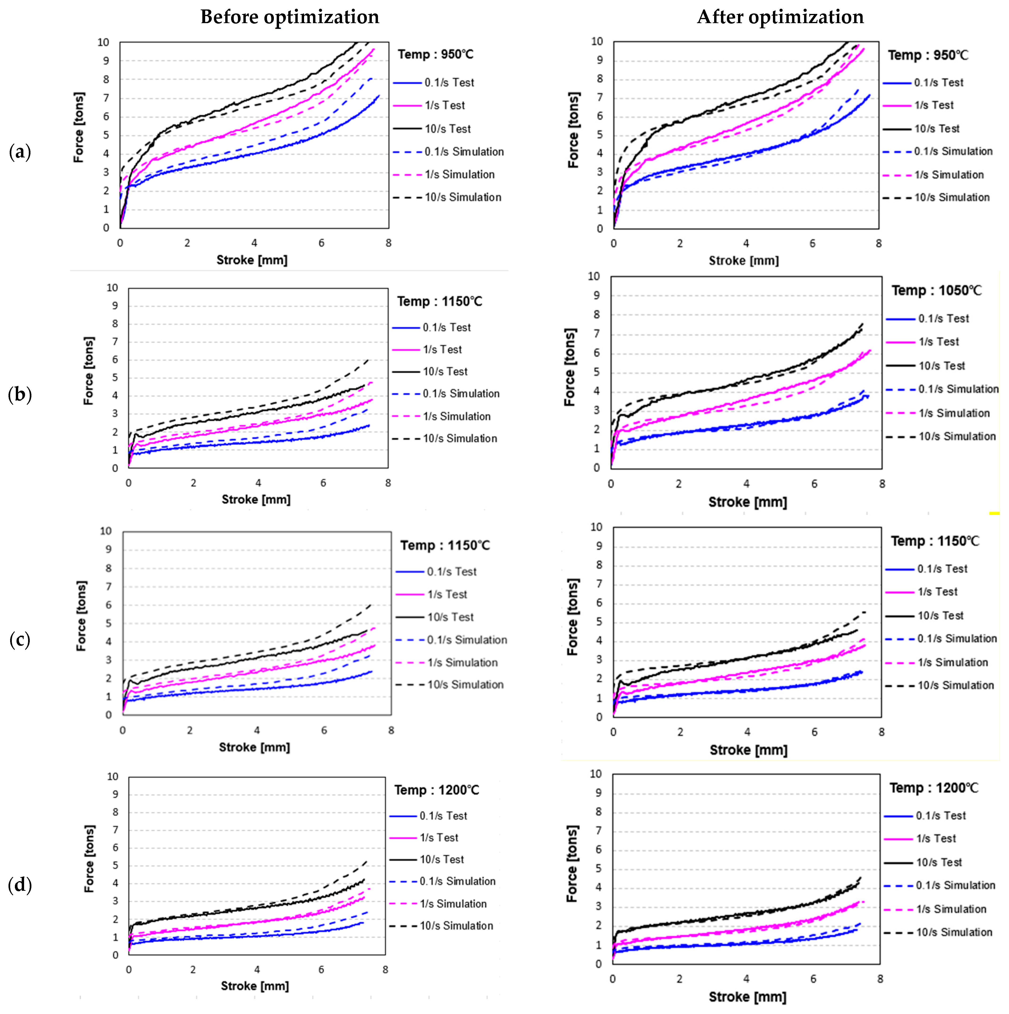
The validity of the flow stress was determined for each temperature condition using the Hansel–Spittel model by minimizing the value of the cost function and evaluating using the same method described in Section 4.1. Here, the optimized flow stress was applied to the Joule heating simulation and compression processes. Figure 11 compares the displacement–load data obtained from the high-temperature Gleeble compression tests with the corresponding simulation results before and after optimization. The simulation results before optimization were calculated using the estimated flow stress based on the Gleeble test results. The simulation results after optimization were obtained using the flow stress optimized for each temperature using the Hansel–Spittel equation. The root mean square error (RMSE) was calculated to quantify both the error of the simulation results before and after optimization and the difference between the experimental and simulated displacement–load curves, as shown in Table 2. The results confirmed that the simulated results were closer to the experimental data after optimization, except for conditions of 10/s at 950 °C and 1/s at 1050 °C. After optimization, the error was reduced by 8.2% to 78.4%, depending on the condition. Overall, the average improvement rate was 34.8%. The RMSE can be expressed as in Equation (9):
5. Conclusions
In this study, the high-temperature flow stress of Inconel 718 was calculated while considering the spatial temperature distribution of the specimen and die, to examine its high-temperature flow behavior. A Joule heating analysis was performed to derive the temperature distribution of the specimen and die. The flow stress was simulated using the Hansel–Spittel model while assuming that the temperature was not uniformly distributed throughout the volume of the specimen prior to compression. The simulated flow stress was then optimized for each temperature condition using the optimization module. The major findings were as follows.
- (1)
- The electrical Joule heating results showed that there was a significant temperature difference between the temperature measurement point and the interface between the specimen and the die. When the deformation temperature was 950 °C, the temperature difference was as large as 70 °C. This means that accurately estimating the flow stress requires analysis of the heating process as well, in addition to the subsequent upsetting analysis.
- (2)
- The optimized flow stress was lower than the calculated value based on the experimental data, and the difference became larger as the deformation temperature increased. This was attributed to the larger difference in temperature between the temperature measurement point and the interface between the specimen and the die at higher deformation temperatures, resulting from Joule heating. This led to a larger deviation from the average temperature of the entire volume of the specimen.
- (3)
- The root mean square error (RMSE) was calculated to quantify the error of the simulation results before and after optimization. Overall, despite the exception under the conditions of 950 °C 10/s and 1050 °C 1/s where the RMSE increased inversely, the RMSE improved by 34.8% on average after optimization, confirming the validity of the optimization process based on Joule heating analysis proposed in the present study.
Author Contributions
Methodology and supervision, J.-H.K.; experiments, H.-C.L.; FE simulation, S.-W.K.; writing, J.-S.P. All authors have read and agreed to the published version of the manuscript.
Funding
This work was supported by the Korea Institute of Energy Technology Evaluation and Planning (KETEP) and the Ministry of Trade, Industry and Energy (MOTIE) of the Republic of Korea (No. 20203010020040).
Institutional Review Board Statement
Not applicable.
Informed Consent Statement
Not applicable.
Data Availability Statement
Not applicable.
Conflicts of Interest
The authors declare no conflict of interest.
References
- Iturbe, A.; Giraud, E.; Hormaetxe, E.; Garay, A.; Germain, G.; Ostolaza, K.; Arrazola, P.J. Mechanical characterization and modelling of Inconel 718 material behavior for machining process assessment. Mater. Sci. Eng. A 2017, 682, 441–453. [Google Scholar] [CrossRef] [Green Version]
- Jonas, J.J.; Sellars, C.M.; Tegart, W.J.M. Strength and structure under hot-working conditions. Metall. Rev. 1969, 14, 1–24. [Google Scholar] [CrossRef]
- Johnson, G.R.; Cook, W.H. Fracture Characteristics of Three Metals Subjected to Various Strains, Strain rates, Temperatures and Pressures. Eng. Frac. Mech. 1985, 21, 31–48. [Google Scholar] [CrossRef]
- Hensel, A.; Spittel, T. Kraft-Und Arbeitsbedarf Bildsamer Formgebungsverfahren, 1st ed.; VEB Deutscher Verlag Für Grundstoffindustrie: Leipzig, Germany, 1978. [Google Scholar]
- Zerille, F.J.; Armstrong, R.W. Dislocation-mechanics-based constitutive relations for material dynamics calculations. J. Appl. Phys. 1987, 61, 1816–1825. [Google Scholar] [CrossRef] [Green Version]
- Khan, A.S.; Liang, R. Behaviors of three BCC metal over a wide range of strain rates and temperatures: Experiments and modeling. Int. J. Plast. 1999, 15, 1089–1109. [Google Scholar] [CrossRef]
- Rao, K.P.; Prasad, Y.K.D.V.; Hawbolt, E.B. Hot deformation studies on a low-carbon steel: Part 1—Flow curves and the constitutive relationship. J. Mater Process Technol. 1996, 56, 897–907. [Google Scholar] [CrossRef]
- Zou, D.N.; Wu, K.; Han, Y.; Zhang, W.; Cheng, B.; Qiao, G.J. Deformation characteristic and prediction of flow stress for as-cast 21Cr economical duplex stainless steel under hot compression. Mater. Des. 2013, 51, 975–982. [Google Scholar] [CrossRef]
- Kang, J.h.; Heo, S.j.; Yoo, J.; Kwon, Y.C. Hot working characteristics of S32760 super duplex stainless steel. J. Mech. Sci. Technol. 2019, 33, 2633–2640. [Google Scholar] [CrossRef]
- Detrois, M.; Antonov, S.; Tin, S.; Jablonski, P.D.; Hawk, J.A. Hot deformation behavior and flow stress modeling of a Ni-based superalloy. Mater. Charact. 2019, 157, 109915. [Google Scholar] [CrossRef]
- Lizzi, F.; Pradeep, K.; Stanojevic, A.; Sommadossi, S.; Poletti, M.C. Hot Deformation Behavior of a Ni-Based Superalloy with Suppressed Precipitation. Metals 2021, 11, 605. [Google Scholar] [CrossRef]
- Grzesik, W.; Nieslony, P.; Laskowski, P. Determination of Material Constitutive Laws for Inconel 718 Superalloy Under Different Strain Rates and Working Temperatures. J. Mater. Eng. Perform. 2017, 26, 5705–5714. [Google Scholar] [CrossRef] [Green Version]
- Park, K.B.; Cho, Y.T.; Jung, Y.G. Determination of Johnson-Cook constitutive equation for Inconel 601. J. Mech. Sci. Technol. 2018, 32, 1569–1574. [Google Scholar] [CrossRef]
- Storchak, M.; Rupp, P.; Moehring, H.C.; Stehle, T. Determination of Johnson–Cook Constitutive Parameters for Cutting Simulations. Metals 2019, 9, 473. [Google Scholar] [CrossRef] [Green Version]
- Liang, Q.; Liu, X.; Li, P.; Ding, P.; Zhang, X. Development and Application of High-Temperature Constitutive Model of HNi55-7-4-2 Alloy. Metals 2020, 10, 1250. [Google Scholar] [CrossRef]
- Wang, H.; Wang, W.; Zhai, R.; Ma, R.; Zhao, J.; Mu, Z. Constitutive Equations for Describing the Warm and Hot Deformation Behavior of 20Cr2Ni4A Alloy Steel. Metals 2020, 10, 1169. [Google Scholar] [CrossRef]
- Peng, X.; Guo, H.; Shi, J.; Qin, C.; Zhao, Z. Constitutive equations for high temperature flow stress of TC4-DT alloy incorporating strain, strain rate and temperature. Mater. Des. 2013, 50, 198–206. [Google Scholar] [CrossRef]
- Yin, F.; Hua, L.; Mao, H.; Han, X. Constitutive modeling for flow behavior of GCr15 steel under hot compression experiments. Matcer. Des. 2013, 43, 393–401. [Google Scholar] [CrossRef]
- Ge, G.; Zhang, L.; Xin, J.; Lin, J.; Aindow, M.; Zhang, L. Constitutive modeling of high temperature flow behavior in a Ti-45Al-8Nb-2Cr-2Mn-0.2Y alloy. Sci. Report. 2018, 8, 1–9. [Google Scholar] [CrossRef] [Green Version]
- Xu, S.; Shu, X.; Li, S.; Chen, J. Flow Stress Curve Modification and Constitutive Model of 20CrMoA Steel during Warm Deformation. Metals 2020, 10, 1602. [Google Scholar] [CrossRef]
- Sekar, K.S.; Kumar, M.P. Optimising Flow Stress Input for Machining Simulations Using Taguchi Methodology. Int. J. Simul. Model. 2012, 11, 17–28. [Google Scholar] [CrossRef]
- Niu, L.; Zhang, Q.; Wang, B.; Han, B.; Li, H.; Mei, T. A modified Hansel-Spittel constitutive equation of Ti-6Al-4V during cogging process. J. Alloys Compd. 2022, 894, 162387. [Google Scholar] [CrossRef]
- Chen, X.; Du, Y.; Du, K.; Lian, T.; Liu, B.; Li, Z.; Zhou, X. Identification of the Constitutive Model Parameters by Inverse Optimization Method and Characterization of Hot Deformation Behavior for Ultra-Supercritical Rotor Steel. Materials 2021, 14, 1958. [Google Scholar] [CrossRef]
- Mirzaie, T.; Mirzadeh, H.; Cabrera, J.M. A simple Zerilli–Armstrong constitutive equation for modeling and prediction of hot deformation flow stress of steels. Mech. Mater. 2016, 94, 38–45. [Google Scholar] [CrossRef] [Green Version]
- Mahalle1, G.; Salunke1, O.; Kotkunde1, N.; Gupta1, A.K.; Singh, S.K. Study of Khan-Huang-Liang (KHL) Anisotropic Deformation Model for Deep Drawing Behaviour of Inconel 718 Alloy. IOP Conf. Ser. Mater. Sci. Eng. 2020, 967, 012054. [Google Scholar] [CrossRef]
- Piao, M.; Huh, H.; Lee, I.; Ahn, K.; Kim, H.; Park, L. Characterization of flow stress at ultra-high strain rates by proper extrapolation with Taylor impact tests. Int. J. Impact Eng. 2016, 91, 142–157. [Google Scholar] [CrossRef]
- Wang, F.; Zhao, J.; Zhu, N. Constitutive Equations and ANN Approach to Predict the Flow Stress of Ti-6Al-4V Alloy Based on ABI Tests. J. Mater. Eng. Perform. 2016, 25, 4875–4884. [Google Scholar] [CrossRef]
- Shang, H.; Wu, P.; Lou, Y.; Wang, J.; Chen, Q. Machine learning-based modeling of the coupling effect of strain rate and temperature on strain hardening for 5182-O aluminum alloy. J. Mater. Proc. Tech. 2022, 302, 117501. [Google Scholar] [CrossRef]
- Li, X.; Roth, C.C.; Mohr, D. Machine-learning based temperature- and rate-dependent plasticity model: Application to analysis of fracture experiments on DP steel. Int. J. Plast. 2019, 118, 320–344. [Google Scholar] [CrossRef]
- Men, Z.; Wang, M.; Ma, Y.; Yue, T.; Liu, R. Application of Direct Resistance Heating in Hot Forging and Analysis of Processing Parameters based on Thermo-electro-mechanical Coupling FEM. High Temp. Mater. Process. 2018, 37, 531–538. [Google Scholar]
- Thangaraju, S.K.; Munisamy, K.M. Electrical and Joule heating relationship investigation using Finite Element Method. IOP Conf. Ser. Mater. Sci. Eng. 2015, 88, 012036. [Google Scholar] [CrossRef] [Green Version]
- Fan, Y.H.; Wang, T.; Hao, Z.P.; Liu, X.Y.; Gao, S.; Li, R.L. Surface residual stress in high speed cutting of superalloy Inconel718based on multiscale simulation. J. Manuf. Proc. 2018, 31, 480–493. [Google Scholar] [CrossRef]
Figure 1.
Heating cycles used for hot compression tests.

Figure 2.
Load and displacement data obtained from compression tests.

Figure 3.
True stress–true strain curves of Inconel 718 from compression tests.

Figure 4.
Input current for heating calculated by heat transfer analysis.

Figure 5.
Temperature simulation results of the material and dies based on Joule heating analysis.

Figure 6.
Conditions related to deformable dies for the Joule heating, heat transfer, and deformation analyses.
Figure 6.
Conditions related to deformable dies for the Joule heating, heat transfer, and deformation analyses.

Figure 7.
Temperature distributions determined by the finite element analysis of Joule heating and the upsetting processes.
Figure 7.
Temperature distributions determined by the finite element analysis of Joule heating and the upsetting processes.
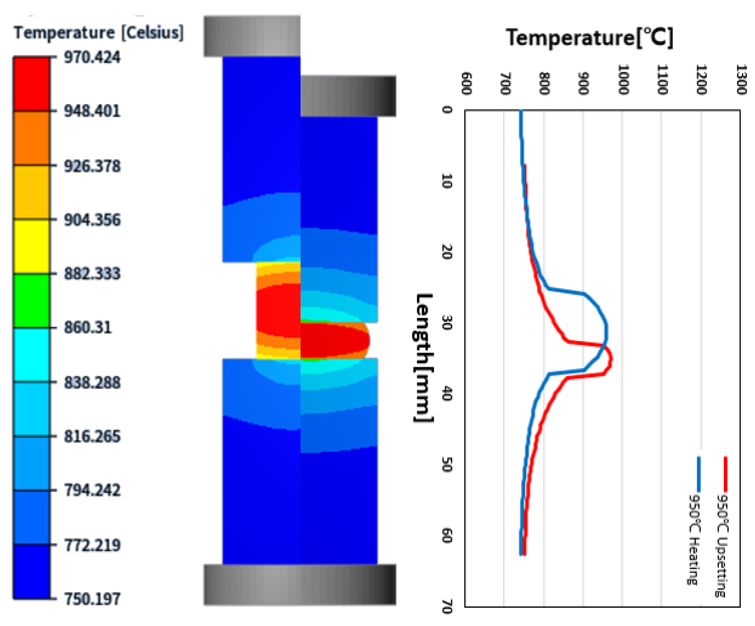
Figure 8.
Comparison of experimental and simulated stroke–force curves without optimization: (a) 950 °C, (b) 1050 °C, (c) 1150 °C, (d) 1200 °C.
Figure 8.
Comparison of experimental and simulated stroke–force curves without optimization: (a) 950 °C, (b) 1050 °C, (c) 1150 °C, (d) 1200 °C.
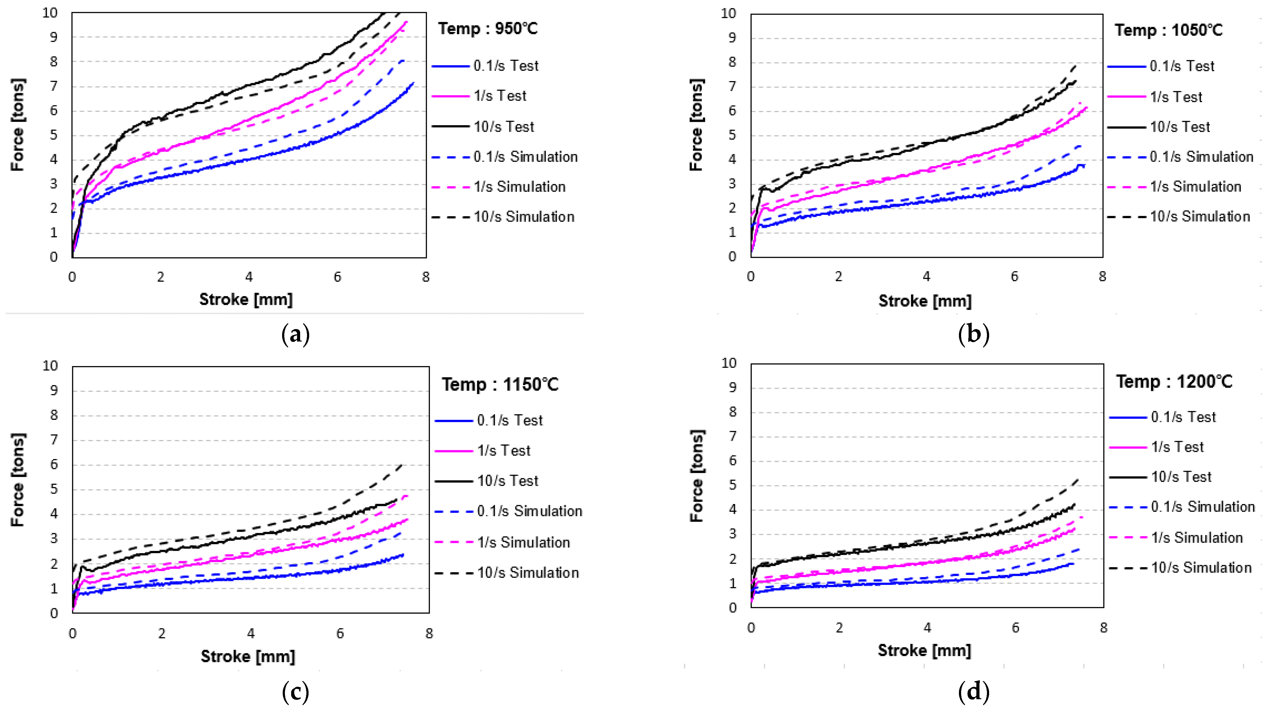
Figure 9.
Changes in cost function and parameters during optimization: (a) cost function, (b) A, (c) m1, (d) m2, (e) m3, and (f) m4.
Figure 9.
Changes in cost function and parameters during optimization: (a) cost function, (b) A, (c) m1, (d) m2, (e) m3, and (f) m4.

Figure 10.
Comparison of flow stress before and after optimization: (a) 950 °C, (b) 1050 °C, (c) 1150 °C, and (d) 1200 °C.
Figure 10.
Comparison of flow stress before and after optimization: (a) 950 °C, (b) 1050 °C, (c) 1150 °C, and (d) 1200 °C.

Figure 11.
Comparison of experimental and analysis results before and after optimization: (a) 950 °C, (b) 1050 °C, (c) 1150 °C, and (d) 1200 °C.
Figure 11.
Comparison of experimental and analysis results before and after optimization: (a) 950 °C, (b) 1050 °C, (c) 1150 °C, and (d) 1200 °C.

Table 1.
Values of A, m1, m2, m3, and m4 parameters after optimization.
| Parameter | Min. | Max. | 950 °C | 1050 °C | 1150 °C | 1200 °C |
|---|---|---|---|---|---|---|
| A | 2000 | 3000 | 2640.9 | 1746.9 | 1458.2 | 1390.0 |
| m1 | −0.02 | −0.001 | −0.00196 | −0.00193 | −0.00197 | −0.00197 |
| m2 | −0.2 | −0.001 | −0.1036 | −0.1378 | −0.1711 | −0.1382 |
| m3 | 0.15 | 0.25 | 0.15 | 0.1692 | 0.1788 | 0.1567 |
| m4 | −0.05 | −0.005 | −0.023 | −0.0197 | −0.0161 | −0.0150 |
Table 2.
Comparison of error of RMSE results before and after optimization.
| Temp. (°C) | Strain Rate (/s) | RMS of Error (MPa) | Difference (MPa) | Improvement Rate (%) | |
|---|---|---|---|---|---|
| Not Optimized | Optimized | ||||
| 950 | 0.1 | 0.5481 | 0.2388 | 0.3093 | 56.4 |
| 1 | 0.3189 | 0.2927 | 0.0262 | 8.2 | |
| 10 | 0.4961 | 0.5132 | −0.0171 | −7.8 | |
| 1050 | 0.1 | 0.3380 | 0.1167 | 0.2213 | 65.5 |
| 1 | 0.2035 | 0.2520 | −0.0485 | −23.8 | |
| 10 | 0.4033 | 0.3672 | 0.0361 | 8.9 | |
| 1150 | 0.1 | 0.3470 | 0.0749 | 0.2721 | 78.4 |
| 1 | 0.2702 | 0.1728 | 0.0974 | 36.0 | |
| 10 | 0.4312 | 0.2390 | 0.1922 | 44.6 | |
| 1200 | 0.1 | 0.2201 | 0.1304 | 0.0897 | 40.8 |
| 1 | 0.1252 | 0.0990 | 0.0262 | 20.9 | |
| 10 | 0.5546 | 0.2786 | 0.2760 | 49.8 | |
| Summary | 4.2562 | 2.7753 | 1.4809 | 34.8 | |
Publisher’s Note: MDPI stays neutral with regard to jurisdictional claims in published maps and institutional affiliations. |
© 2022 by the authors. Licensee MDPI, Basel, Switzerland. This article is an open access article distributed under the terms and conditions of the Creative Commons Attribution (CC BY) license (https://creativecommons.org/licenses/by/4.0/).
Share and Cite
MDPI and ACS Style
Park, J.-S.; Kim, S.-W.; Lim, H.-C.; Kang, J.-H. Flow Stress Optimization of Inconel 718 Based on a Coupled Simulation of Material-Forming Analysis and Joule Heating Analysis. Metals 2022, 12, 2024. https://doi.org/10.3390/met12122024
AMA Style
Park J-S, Kim S-W, Lim H-C, Kang J-H. Flow Stress Optimization of Inconel 718 Based on a Coupled Simulation of Material-Forming Analysis and Joule Heating Analysis. Metals. 2022; 12(12):2024. https://doi.org/10.3390/met12122024
Chicago/Turabian StylePark, Jong-Soo, Seung-Woo Kim, Hyung-Cheol Lim, and Jong-Hun Kang. 2022. "Flow Stress Optimization of Inconel 718 Based on a Coupled Simulation of Material-Forming Analysis and Joule Heating Analysis" Metals 12, no. 12: 2024. https://doi.org/10.3390/met12122024
Note that from the first issue of 2016, this journal uses article numbers instead of page numbers. See further details here.