
Effect of EMBr on Flow in Slab Continuous Casting Mold and Industrial Experiment of Nail Dipping Measurement

1
Hebei Provincial High-Quality Steel Continuous-Casting Engineering Technology Research Center, Tangshan 063000, China
2
College of Metallurgy and Energy, North China University of Science and Technology, Tangshan 063009, China
3
School of Science and Engineering, Hebei University of Science and Technology, Shijiazhuang 050018, China
*
Authors to whom correspondence should be addressed.
Metals 2023, 13(1), 167; https://doi.org/10.3390/met13010167
Submission received: 1 December 2022
/
Revised: 10 January 2023
/
Accepted: 11 January 2023
/
Published: 13 January 2023
Abstract
:In this study, a funnel mold (FM) model of a multi-mode electromagnetic braking (EMBr) device was developed, and the magnetic flux density at different currents was obtained by MAXWELL software. By using the magnetohydrodynamics (MHD) module of FLUENT software, the volume of fluid binomial flow turbulence model and the EMBr mathematical model of the steel/slag flow field were coupled, and the characteristics of the molten steel flow and the liquid-level fluctuation in the 1520 mm × 90 mm FM with the casting speed of 6 m/min were calculated under the effect of the electromagnetic field. The FM liquid-level characteristic information under production conditions was obtained in a nail board industrial experiment and compared with the magnetic-fluid coupling model. The results show that the EMBr can significantly change the flow behavior of molten steel. When the magnetic pole current is not less than 800-600 A, the maximum liquid-level fluctuation height decreases from 18 mm without EMBr to less than 5 mm, and the liquid-level cannot easily entrap slag. Considering the EMBr effect and production cost, the reasonable magnetic pole current should be 800-600 A. The reliability of numerical simulation was also verified by the industrial test results of the nail board.
1. Introduction
In the continuous-casting process, the flow state of molten steel in the mold has a great influence on the quality of the billet. Especially in the casting of a thin-slab with high casting speed, the velocity of molten steel from the outlet is large, the steel/slag interface fluctuates violently, and the molten steel flowing down at high speed easily leads to bubbles and non-metallic inclusions into a deeper position in the mold, which are trapped by the solidified shell and cause defects such as cracks, sliver defects and remelting [1,2,3]. To avoid slag entrapment on the liquid-level and control steel/slag interface fluctuation, the surface velocity of molten steel should be controlled in a reasonable range. Equipment which controls fluid flow in the mold through the application of static magnetic fields is referred to as an electromagnetic braking (EMBr) device under the condition of high casting speed. EMBr can effectively restrain the scouring of the narrow face (NF) of the mold by the submerged entry nozzle (SEN) outlet flow and then stabilize the liquid-level fluctuation of molten steel [4,5,6].
To date, EMBr has been developed into three common types: Local EMBr, Ruler-EMBr and flow control mold (FC-Mold) EMBr [7,8,9,10]. In Local EMBr, two separate magnets are located near the SEN ports, mainly to suppress molten steel velocity from the nozzle and prevent mold flux entrapment. Ruler-EMBr utilizes one pair of magnets, which covers the entire wide faces of the mold, with the aim to stabilize the surface velocity and prevent slag entrapment [11,12]. To better control liquid-level fluctuations and molten steel flow behavior in the mold, a third-generation electromagnetic braking (FC-Mold EMBr) device was proposed. The FC-Mold EMBr device consists of two pairs of magnets across each wide face. One is located on the liquid-level of the FM, and the other is located below the SEN port. Compared with Local EMBr and Rule-EMBr, FC-Mold EMBr can better control surface velocity and liquid-level fluctuation. However, due to its large installation space, complex equipment and difficult maintenance, it is not suitable for thin-slab continuous casting [13]. However, with the increasing casting speed of the thin-slab continuous caster, the above EMBr device has some shortcomings. For example, the braking effects of Ruler-EMBr on the surface velocity and level fluctuation are not significant, and Ruler-EMBr is usually unable to suppress mold slag entrapment effectively [14]. Therefore, a multi-mode EMBr device has been rapidly developed according to the different shapes of the SEN outlet and liquid steel flow-field pattern in an attempt to control the local flow-field pattern and flexible installation of its magnetic pole position. An example is the vertical electromagnetic brake (in which two pairs of magnetic poles are installed vertically on the mold wide sides close to the NF) [15].
In the actual production process, the thickness of the liquid-slag layer, the profile of the liquid-level and the flow direction of the molten steel have important reference value for the production operation, so it is very important to obtain the information of the liquid- level [16,17]. The fluid flow pattern in the mold is difficult to measure, owing to the harsh molten steel/slag environment and electrical interference, such as from electromagnetic flow control systems [18]. Therefore, the application of the nail board is very important because, due to its adaptability, it can easily and quickly obtain the mold liquid-level information. This method is widely used in major steel mills.
In this study, a finite element model based on MAXWELL software was used for the calculation of electromagnetic fields in order to calculate the magnetic field distribution. In addition, a three-dimensional (3D) mathematical model of fluid flow was developed based on FLUENT software using the finite volume method. A magnetohydrodynamics (MHD) module included in FLUENT software was used to import magnetic field data, which were then coupled to the flow fields to determine the effect of electromagnetic braking (EMBr) on fluid flow in a flexible thin-slab caster (FTSC) funnel mold (FM). The production data of the FM liquid-level were obtained through the industrial test of the nail board, and the numerical simulation results were verified.
2. Mathematical Model
2.1. Basic Assumptions
- (1)
- The molten steel flow in the FM is viscous and incompressible.
- (2)
- The molten steel is considered to be homogeneous, with constant thermophysical properties.
- (3)
- The influence of factors such as FM vibration on the flow field is not considered.
- (4)
- The density difference after solidification of the slab is ignored, and the molten steel in the FM is treated as a homogeneous medium.
- (5)
- The electromagnetic characteristics of liquid steel are uniform and isotropic, and the secondary magnetic field generated in the molten steel is ignored.
2.2. Electromagnetic Force Equation
Multi-mode EMBr technology has gradually developed in recent years. Therefore, in this study, a multi-mode EMBr device was suitably designed for a FTSC FM, which was realized through five constant magnetic fields distributed on an entire wide face. The EMBr device consists of five pairs of stable N-S poles wound by a certain number of coils to which a direct current is applied. The geometric model of the EMBr device of the FTSC FM and magnetic pole names are shown in Figure 1. Figure 2 shows that the upper part of the FM has two pairs of magnetic poles, distributed on both sides of SEN. There are three pairs of magnetic poles at the lower part of the SEN, two pairs of magnetic poles are installed under the SEN outlet side and one pair of magnetic poles is installed at the outlet directly below the SEN. The static magnetic field formed by the magnetic poles on both sides of the SEN can comprehensively control the downward and upward tributaries formed by the outlet at the SEN side, and the static magnetic field generated by the magnetic pole directly below can control the flow velocity of the outlet directly below SEN.
It is of great importance to solve for the induced current density when studying the interaction between the movement of conducting molten steel and an applied magnetic field. Here, the electrical potential method was adopted to calculate the induced current density and electromagnetic force based on Ohm’s law and MAXWELL’s equations. The induced current density is given by Ohm’s law [21]:
where B is the magnetic flux density with the unit of T, j is the induced current density in A/m2, E is the electric field intensity in V/m, m is the fluid velocity with the unit of m/s and is the electrical conductivity with the unit of S/m.
In general, the influence of a secondary magnetic field is ignored for the calculation of the static magnetic field. By introducing the electrical potential , the electric field intensity [22,23,24,25] can be expressed as:
According to charge conservation:
Hence, the potential equation can be expressed as:
The electromagnetic force F is obtained with the following equation:
2.3. Flow-Field Governing Equation
The 3D geometric models of the FM and SEN were developed using SOLIDWORKS software, as shown in Figure 3a,b. Molten steel in the FM is a 3D incompressible fluid, and its flow control equations include the continuity equation, momentum equation and turbulence model equation. The turbulence model used in this study is the standard k-ε equation, and the specific equations are described in Equations (6)–(10) [26,27,28,29].
(1). Continuity equation:
where is the density of molten steel in kg/m3 and is the fluid velocity in the direction with the unit of m/s.
(2). N-S equation:
where p is the pressure with the unit of Pa and is the effective viscosity coefficient with the unit of Pa·s, is an additional force in N.
(3). k–ε turbulence model:
Turbulent kinetic energy equation:
Dissipation rate of turbulent kinetic energy:
The effective viscosity is expressed as:
where , = 1.44, = 1.92, = 0.09, = 1.0 and = 1.3.
In the simulation of the FM steel/slag interface, the volume of fluid (VOF) method was used to track the steel/slag interface, define the fluid volume fraction in the space grid of the moving interface, construct the development equation of the fluid volume fraction, track the changes of the interface, determine the position and shape of the steel/slag interface and thus construct the steel/slag interface [30].
(1). Continuity equation:
where is time in s, is the density of molten steel in kg/m3 and is the fluid velocity in the direction with the unit of m/s.
(2). N-S equation:
where p is the pressure with the unit of Pa, and is the gravitational force vector in m/s2.
The VOF model was employed to solve the multiphase steel/slag system. This scheme performs the calculation of the interface between the phases ( and q) present at each cell, based on their fraction as follows [31,32,33]:
where is the volume fraction, and q are phases in a multiphase flow, is the volume source phase, 1/s. and are the volume change phases caused by mass transfer between phase to phase and phase to phase per unit time per unit volume, respectively, 1/s.
The constraint condition of the mathematical equation in the VOF model is that the sum of each relative volume fraction is 1, and the expression of the constraint equation is as follows:
where, is the volume fraction of each phase.
2.4. Boundary Conditions and Numerical Calculation
The static electromagnetic field was solved by MAXWELL software. The boundary conditions for the magnetic field calculation are simple, and only the parallel magnetic flux condition at the air interface needs to be set.
The FM flow field was solved by FLUENT software. To reduce the calculation time, according to the symmetry of the flow in the FM, the calculation area was taken as 1/4 of the FM flow area for simulation calculation. To avoid the influence of reflux on the calculation accuracy, the length of the calculating FM domain was determined to be 2200 mm by trial calculation. The MESH module of ANSYS software was used to divide the model. Tetrahedral unstructured cells and hexahedral cells were used, and the FM liquid-level domain was encrypted. The mesh-independent verification of the calculation results was carried out, and the number of cells of the SEN FM model was determined to be about 1.2 million; see Figure 4.
The boundary conditions of the FM flow field are as follows: (1). The SEN inlet is defined as the velocity inlet. The velocity as determined by the casting speed is obtained according to the flow rate balance of molten steel.
Determination of turbulent kinetic energy K and turbulent kinetic energy dissipation rate [34] is turbulence intensity I [35]. I is expressed by:
The turbulent kinetic energy and corresponding dissipation rate are expressed by:
Re is the Reynolds number, the hydraulic diameter of DH is 80 mm and v is the kinematic viscosity of molten steel.
(2). Symmetry faces: The velocity and current density components perpendicular to the symmetry faces and the normal gradient of the other variables are set to zero.
(3). Top surface: The top surface is defined as the free surface with a free slip. The slag layer is 30 mm.
(4). Outlet of FM: The exit of the FM is defined as the pressure outlet with a gage pressure of zero. The backflow values of other variables are considered to be constant.
(5). Walls: Both walls of the FM and the SEN are considered to be non-slip standard walls with normal velocity and current density components of zero. Normal components of other variables are also taken as zero.
The electromagnetic field boundary conditions were set in FLUENT software as follows:
Meniscus and FM walls are considered as insulated walls as follows:
At the symmetry plane and boundary at the end of casting direction, electrical potential was set to 0, and the electromagnetic force was obtained by the Equation (5). The governing Equation (4) was discretized using the finite element method. Equations (6)–(9) were discretized using the finite volume approach. The SIMPLE algorithm based on pressure-velocity coupling was employed to solve these equations. The residual value used for judging whether the solution is convergent was set to 105. On the basis of the above analysis, the method of solution is summarized as follows [19,36,37,38,39].
(1). The magnetic field distribution in the FM was calculated using the finite element MAXWELL software.
(2). Magnetic field data were imported to the activated MHD module to couple the magnetic field with the flow fields.
(3). The SIMPLE algorithm was adopted to solve the algebraic equations to obtain the coupling to pressure and velocity.
(4). Calculations were iterated until a residual value of less than 105 was achieved.
Parameters used in physical and numerical simulations are presented in Table 1.
2.5. Validation of Models
To verify the accuracy of the numerical simulation of the electromagnetic field, the magnetic flux density in the air domain of the FM (width × thickness × height: 1520 mm × 90 mm × 1200 mm) was actually measured under the condition of field shutdown for maintenance. The magnitude of current through the EMBr device was measured as shown in Table 2.
The measurement method is to carry out equal-spaced 9 × 9 meshing points in each section width and height direction from the area 230 mm away from the upper end of the FM and 200 mm away from the lower end of the FM on both sides of the 1/4 section and the middle section along the width direction of the FM and measure one by one. Due to the symmetry of the magnetic field of the FM, the average value of the symmetrical value is processed after the measurement, and the singularity caused by the measurement error is omitted.
The measuring process and measuring points are shown in Figure 5a,b.
To make the numerical simulation results of the electromagnetic field consistent with the actual measurement results, the MAXWELL software was used to perform numerical simulation of the electromagnetic field for the current combinations numbered as groups 1 to 3. After continuous improvement of the mathematical model of the electromagnetic field, the simulation results of the mathematical model were in good agreement with the field measurement results. Taking the current combination under the condition of group 2 as an example, this article describes in detail the checking method of the numerical simulation and actual measurement results. That is, the magnetic flux density data of feature lines 1 and 2 on the middle section of the cloud image were extracted and compared with the magnetic flux density values of the same position measured in the field. The solved FM static magnetic field vector diagram and cloud diagram are shown in Figure 6 and Figure 7. Figure 8 shows that the numerical simulation results are in good agreement with the measured results.
3. Results and Discussion
The magnetic flux density is generally only related to the magnitude of current and the number of coil turns and has no obvious relationship with the height [42]. With other parameters unchanged, this work only solved the magnetic flux density of the FM under different current parameter conditions and then applied the magnetic flux density to the molten steel flow field of the FM to study the influence of magnetic flux density on the molten steel flow field. The numerical simulations in the present work involve the coupling of the magnetic field and the flow field, which should provide a useful reference in actual production environments.
3.1. Electromagnetic Field Calculations
The distribution of magnetic flux density in the FM can be obtained by numerical simulation of the direct current static electromagnetic field. Figure 9 shows the distribution of magnetic flux density at five pairs of magnetic poles at the center section of the width face of the FM under different current parameter conditions.
As can be seen from Figure 9, the magnetic flux density of the two A/C poles are the same, and the magnetic flux density is the largest because the current through the coil of the two magnetic poles is the largest, and the magnetic yoke area is the largest. According to the Faraday law of electromagnetic induction, it can be seen that the A/C poles generate the strongest magnetic flux density. The magnetic flux density of the two poles of D/E are also the same, but the magnetic induction value is the lowest, and the magnetic induction value of F magnetic pole is in the middle. The reason why the magnetic flux density of the D/E poles are smaller than that of the F pole is that in the three magnetic poles of D/E/F, the magnetic flux of the two magnetic poles of D/E gathers at the F pole in the process of forming a loop, which strengthens the magnetic flux density of the F pole [43]. Since the current direction of A/C poles is opposite to that of D/E/F poles, in the form of a magnetic flux loop, at the lower part of the A/C poles and the junction of the upper part of the D/E/F poles, part of the magnetic flux offset, in the FM longitudinal direction, the formation of a shape similar to the inverted “Ω” of the geometric magnetic field distribution occurs, in line with the SEN molten steel flow electromagnetic field distribution.
As shown in Figure 10, the magnetic flux density of each magnetic pole increases with the increase in the current, and the magnetic flux density gradually decreases from the center area of the magnetic yoke to the periphery. Under the condition of 300-200 A, the magnetic flux density value in the central region of the magnetic yoke is about 70 mT. When the current is 1100-800 A, the magnetic flux density value in the central region of the magnetic yoke is about 200 mT. It can be seen that the magnetic flux density increases significantly with the increase in current.
3.2. The Influence of EMBr on Flow Pattern of Molten Steel
Figure 11 shows the influence of different magnetic flux density on the molten steel flow field in the FM with different magnitudes of current at the submergence depth of 160 mm and the casting speed of 6 m/min. As shown in Figure 11, with the increase in the current, the red flow strands at the outlet of the SEN gradually shorten, and the velocity of the molten steel jet decreases gradually. As a result, after the SEN jet impacts the NF of the FM, the velocity of the upper and lower strands formed by the nozzle jet decreases; thus, the surface velocity decreases.
Compared with the molten steel flow field without EMBr, when the current is 300-200 A, due to the effect of EMBr, the kinetic energy of the SEN jet decreases, and the upper and lower strands start to form at the jet terminal far away from the NF of the FM, which reduces the impact of the jet on the NF. When the current is 800-600 A, the EMBr effect is enhanced, and the kinetic energy of the SEN jet decreases obviously. However, it can still flow through the following pair of magnetic poles, and the jet terminal moves down obviously. When the current is 1100-800 A, due to the enhanced EMBr effect of the upper and lower magnetic stages, the jet slows down significantly when passing through the lower magnetic pole, forming upper and lower strands at the upper part of the jet terminal at 800-600 A. However, compared with other molten steel flow fields without EMBr and 300-200 A, the jet terminal still drops further.
In addition, it can be seen from the cloud images that compared with the molten steel flow field without EMBr, after EMBr is applied, the flow-field area of the molten steel jet path velocity at the nozzle in the FM expands. However, compared with the molten steel main jet without EMBr, the velocity gradient is significantly reduced, which can reduce the turbulence of molten steel in the FM and make the flow-field distribution of molten steel in the FM more uniform and reasonable.
Figure 12 shows the velocity cloud image and vector image of the FM at the submergence depth of 160 mm and the casting speed of 6 m/min. Figure 12 shows that under the condition that no EMBr is applied, the main position of the SEN jet impinges on the NF of the FM in the lower part of the FM, while the velocity in the upper part is low, and the maximum velocity of the NF is about 0.46 m/s. When the EMBr is applied, with the increase in magnetic flux density, the velocity in the lower part of the FM NF decreases gradually compared with the result without EMBr. However, when the EMBr is applied at the beginning (the current is 300-200 A), the magnetic flux density is strengthened, and the velocity of the main jet in the lower region begins to weaken, but it cannot sufficiently reduce the kinetic energy of the main jet, which leads to the partial kinetic energy of the main jet being transferred to the up-moving tributaries, and then the velocity on the NF is strengthened. With the increase in the current, the magnetic flux density is further strengthened, and the velocity of the NF and the lower region begin to gradually weaken. However, when the current is 800-600 A, the velocity of the NF is higher than that of the lower region. When the current is 1100-800 A, the face is the strongest, and the NF velocity is the lowest, and its maximum value is about 0.21 m/s. It can be seen from the NF velocity cloud image and vector image that the NF velocity is greatly reduced after EMBr is applied, effectively reducing the impact of the jet on the solidified shell of the slab along with the probability of the solidified shell remelting, cracks and other quality defects [44].
Figure 13 shows that when the submergence depth is 160 mm and the casting speed is 6 m/min, with the increase in current, the surface velocity of FM liquid-level gradually decreases in the central region, the area near the NF and the SEN region. Figure 14 shows that the maximum surface velocity decreases from 0.49 m/s without EMBr to 0.32 m/s when the EMBr current is 1100-800 A. It can be seen that the application of EMBr can effectively restrain the excessive surface velocity of molten steel.
3.3. Influence of Magnetic Flux Density on Liquid-Level Shape of Steel/Slag
Figure 15 and Figure 16 show the maximum liquid-level fluctuation at different times and the liquid-level slag entrapment diagram with a steel/slag volume fraction of 0.5. As shown in Figure 15, in the case of no EMBr, when the SEN submergence depth is 160 mm and the casting speed is 6 m/min, within 0–30 s, the fluctuation of the whole liquid-level is extremely unstable, and the fluctuation value of the liquid-level at multiple time points reaches more than 10 mm and the maximum value even reaches 17.4 mm. In this case, the liquid-level is prone to slag entrapment. Moreover, the slag entrapment area has a large range; see Figure 16a. When the EMBr is applied, the effect of EMBr is enhanced with the increase in current, and the fluctuation of liquid-level decreases gradually. However, when the current is 300-200 A, the maximum fluctuation of the liquid-level can still reach about 14 mm, and there are multiple, serious occurrences of slag entrapment on the liquid -level. When the current is 800-600 A, the whole liquid-level becomes relatively stable, the liquid-level fluctuation value is basically less than 5 mm and the probability of slag entrapment is very small. Even if slag entrapment occurs, the slag entrapment area is small. When the current reaches 1100-800 A, the fluctuation value of the liquid-level is about 2 mm, the liquid-level is extremely stable and there is basically no slag entrapment at the liquid-level. However, the braking effect of EMBr is too strong, the upper stream cannot reach the liquid-level or the distance from the liquid-level is too large, the liquid-level is too calm, which has a serious impact on the heat supply of molten steel at the liquid-level, affecting the melting of the slag and having a series of adverse effects on the production [45,46].
3.4. Industrial Test
3.4.1. Nail Dipping Measurement
The nail board test is a fast and efficient method to obtain the information of the liquid-level.
To keep the nails horizontal and stable in the dipping tests, one end of the nails used is inserted into the wood board. Each stainless nail has a length of 150 mm and a diameter of 5 mm, spaced 70 mm apart and attached to the wood board, together with 3 mm diameter aluminum nails. This is shown in Figure 17a, and the dipping position is shown in Figure 17b.
The SEN side and NF side were marked before measurement; see Figure 18a. Based on the data of computational modeling by Rietow and Thomas [47], during dipping tests, the molten steel solidifies on the nail surface after staying for about 2–3 s and lifting vertically. As molten steel flows around the nails, it is pushed up on the windward side, and down on the leeward side, so an angled lump solidifies around each nail. As shown in Figure 18b, after taking out the nails from the molten steel pool, these solidified steel lumps are used to reveal the liquid-level profile and the velocity across the top of the FM. Surface velocity vs at the nail is estimated from the measured lump height difference h, and lump diameter d, as shown in Figure 18b, using the empirical Equation (19) developed by Liu et al. [48,49].
where vs is the surface velocity in m/s, d is lump diameter in mm and h is the lump height difference with the unit of mm.
By measuring the distance Hsteel between the highest point and the end of solidified steel lump, the height of the liquid-level at different times and positions in the FM can be obtained. The liquid-level profiles at different times can be obtained by connecting the liquid-level heights of each point. The flow direction of the molten steel is the direction from the top end of the solidification lump to the lowest point [50]. In addition, since the melting point of aluminum is 660 °C, which is lower than the liquid-slag layer temperature, the inserted aluminum nail melts in the liquid-slag layer. Liquid-slag layer thickness (Hslag) can be obtained according to the height difference between steel nails and aluminum nails; see Figure 18b.
The low carbon steel was used as the experimental steel grade, its size is 1520 mm × 90 mm (width × thickness), the casting speed is 6 m/min, the SEN submergence depth is 160 mm and the current conditions are no EMBr, 300-200, 800-600 and 1100-800 A. The nail board test was carried out at the liquid-level of the FM. During the measurement, at the same position of the liquid-level of the FM, three consecutive measurements were made, each at intervals of 3 min, and the average value was taken. The furnace times measured by the nail board do not include the pouring or stopping processes.
3.4.2. Test Results of Molten Steel Flow at Liquid-Level
As shown in Figure 19, on the FM wide face, the surface velocity presents a parabolic shape, and the maximum surface velocity appears at the distance of 0.3–0.5 m from the SEN. Without the EMBr applied, the maximum surface velocity is about 0.46 m/s, and the maximum value is about 0.4 m away from the SEN. After the use of the EMBr device, the position of the maximum surface velocity changes. The larger the current, the closer the maximum surface velocity position is to the NF of the FM, and the maximum surface velocity value decreases with the increase in the current. The reason is that when the SEN jet passes through the magnetic field between the upper magnetic poles for the first time, the kinetic energy of the jet decreases. When the upper and lower tributaries are formed, the upward tributaries pass through the magnetic field between the upper magnetic poles for the second time, and the kinetic energy of the tributaries decreases again. The greater the current, the more obvious the kinetic energy decreases, and the shorter the upward flow of the tributary. When the magnetic pole current increases to 1100-800 A, the maximum surface velocity decreases from about 0.46 m/s without EMBr to about 0.25 m/s, a decrease of about 46%. The results show that the numerical simulation is in good agreement with the industrial test.
Figure 20 is a vector diagram of molten steel flow at the FM liquid-level. The arrow direction represents the flow direction, and the arrow length represents the velocity of the molten steel. The Figure shows that the main flow direction of molten steel is from the NF to the SEN. As shown in Figure 20, when there is no EMBr and the current is 300-200 A, the arrow is longer, indicating the surface velocity is larger. The arrows are disordered, and the direction of the molten steel flow at the surface is disordered. In the area about 300 mm away from the SEN, the arrow points from the SEN to the NF direction, which indicates that the direction of molten steel flow is opposite to that of the mainstream flow. Therefore, it can be inferred that there is turbulence pulsation in part of the liquid-level, a vortex is generated in this position when the nail is inserted and the nail is on the rotating side of the vortex pointing from the SEN to the NF. At this time, slag entrapment very easily occurs at the liquid-level. As the current of the EMBr device increases, the arrows gradually become orderly and stable, and the arrows become shorter and shorter. The results show that the liquid-level velocity decreases, the turbulence weakens, and the liquid-level flow field is stable. When the current reaches 800-600 A, the liquid-level is very stable. When the current reaches 1100-800 A, the liquid-level is more stable, but with excessive current, the liquid-level activity decreases, which is not conducive to the melting of slag. The vector diagram shows that EMBr can not only reduce the liquid-level surface velocity but also make the flow field more regular.
3.4.3. Test Results of Liquid-Level Profile
The instantaneous Hsteel value of the average height of the nail was measured three times under different magnetic current conditions. Figure 21 shows the liquid-level waveform on the centerline of the wide face obtained by connecting the Hsteel values of each point.
Figure 22 is the instantaneous distribution of the thickness of the liquid-slag layer measured on the center line of the wide face.
As shown in Figure 21, the liquid-level at the SEN of the FM is relatively low, while the liquid-level near the NF is relatively high. The average height of the overall liquid-level is about 60 mm. However, with the increase in the current, the difference of the liquid level between the SEN side and the NF becomes smaller and smaller. The height difference decreases from 31 mm without EMBr to 23.5 mm at 300-200 A, 7.2 mm at 800-600 A and 6.1 mm at 1100-800 A. The results show that after EMBr is applied, the effect of EMBr is continuously strengthened with the increase in current, the kinetic energy of the upflowing strand impacting the liquid-level becomes smaller and smaller and the liquid level becomes increasingly stable. Compared with the numerical simulation results, the liquid-level waveform is also very similar on the whole. That is, the SEN side is low, and the NF is high. The greater the current, the more stable the entire liquid-level height difference.
The liquid-slag layer image is opposite to the waveform image, that is, the higher the liquid-level waveform, the thinner the liquid-slag layer. The reason is that the higher the liquid-level waveform, the stronger the shear action on the liquid-slag layer, resulting in the liquid-slag layer thinning [51,52]. However, if the effect of EMBr is too strong, the liquid-level molten steel is not active enough to supplement the slag heat. For example, although the thickness of liquid-slag layer in Figure 22d is more uniform than that in Figure 22c, it is not as thick as that in Figure 22c. Therefore, it is very important to determine the magnitude of current reasonably to obtain the appropriate liquid-slag layer thickness [53].
4. Conclusions
In this work, the relationship between the magnetic flux density of the FM multi-mode EMBr device and the magnetic pole current was simulated and studied. The different magnetic flux density data were coupled with the FM flowfield model through the MHD module of the FLUNET software, the influence of the magnetic pole current on the molten steel flow field in the FM was studied and a magnetic-fluid coupling model was verified by industrial testing of the nail board. The conclusions were drawn as follows:
(1) The magnetic flux density of the FM increases with the increase in magnetic pole current. When the magnetic current reaches 1100-800 A, the magnetic flux density in the FM reaches about 200 mT.
(2) EMBr can significantly change the flow behavior of molten steel in the FM. With the increase in magnetic flux density in the FM, the surface velocity decreases gradually. The maximum surface velocity decreases from 0.49 m/s without EMBr to 0.32 m/s when the EMBr current is 1100-800 A. The application of EMBr can effectively restrain the excessive surface velocity of molten steel.
(3) After the EMBr is applied, the impact of the molten steel flow strand on the NF of the FM is reduced from about 0.46 m/s without EMBr to 0.17 m/s when the current is 1100-800 A, and the probability of continuous-casting leakage is reduced.
(4) When the magnetic pole current is not less than 800-600 A, the maximum liquid-level fluctuation height decreases from 18 mm without EMBr to less than 5 mm, and flow-field distribution is more reasonable. Considering the EMBr effect and production cost, the reasonable magnetic pole current should be 800-600 A.
(5) According to the industrial test of the nail plate, the liquid-level of the FM becomes stable and orderly after the EMBr equipment is included, and the test results are in good agreement with the simulation results.
(6) To achieve high efficiency and stable operation of continuous-casting production, it is recommended to use the EMBr device to control the flow of molten steel in the 1520 mm × 90 mm FM with the casting speed of 6 m/min. The magnetic current should be controlled between 800-600 and 1100-800 A. This can achieve the ideal braking effect and consume less electric energy at the same time. The result can provide a certain theoretical reference for the actual production.
Author Contributions
L.Z. (Limin Zhang): Writing—original draft, writing—review and editing, conduct experiment, data, graphics; P.X.: Contact with the plant; Y.W.: Funding, review; C.Z.: Contact with the plant, formal analysis; L.Z. (Liguang Zhu): Project administration, methodology, review, funding, goals and aims. All authors have read and agreed to the published version of the manuscript.
Funding
This work was funded by the National Natural Science Foundation of China—Regional Innovation and Development Joint Fund key project (Grant No. U21A20114), the Nature Science Foundations of Hebei (Grant No. CXZZBS2020130, No. E2020209005, No.2021209037, No. E2019209543), the National Natural Science Foundation of China (Grant No. 51904107, No. 52004094, No. 51974133), Tangshan Talent Subsidy project (Grant No. A202010004), the Science and Technology Research Project of Colleges and Universities of Hebei Province (Grant No. BJ2019041) and the Hebei Province “Three Three Three Talent Project” (Grant No. A202010004).
Institutional Review Board Statement
Not applicable.
Informed Consent Statement
Not applicable.
Data Availability Statement
Not applicable.
Conflicts of Interest
The authors declare no conflict of interest.
Abbreviations
| Acronyms | Words |
| FM | funnel mold |
| EMBr | electromagnetic braking |
| MHD | magnetohydrodynamics |
| NF | narrow face |
| SEN | submerged entry nozzle |
| FC-Mold | flow control mold |
| 3D | three-dimensional |
| FTSC | flexible thin-slab caster |
| VOF | volume of fluid |
References
- Thomas, B.G. Modeling of Continuous Casting Defects Related to Mold Fluid Flow. Iron Steel Technol. 2006, 3, 128–143. [Google Scholar]
- Zhang, L.M.; Zhu, L.G.; Tian, P.; Xiao, P.C.; Liu, Z.X.; Zhang, C.J. Analysis and control of peeling defects of 65Mn steel in cold rolling. Steelmaking 2020, 36, 63–69. [Google Scholar]
- Zheng, S.G.; Zhu, M.Y. Study on mechanism of mold powder entrapment in funnel type mould of flexible thin slab casting machine. Ironmak. Steelmak. 2014, 41, 507–513. [Google Scholar] [CrossRef]
- Yavuz, M.M. The Effects of Electromagnetic Brake on Liquid Steel Flow in Thin Slab Caster. Steel Res. Int. 2011, 82, 809–818. [Google Scholar] [CrossRef]
- Zhu, L.G.; Zhang, L.M.; Wang, X.J.; Zhang, C.J.; Han, Y.H.; Sun, L.G. Physical experiment and numerical simulation of flow field on funnel mold surface. Contin. Cast. 2021, 6, 2–8. [Google Scholar]
- Hibbeler, L.C.; Thomas, B.G. Mold Slag Entrainment Mechanisms in Continuous Casting Molds. Iron Steel Technol. 2013, 10, 121–134. [Google Scholar]
- Cho, S.M.; Kim, S.H.; Thomas, B.G. Transient Fluid Flow during Steady Continuous Casting of Steel Slabs: Part I. Measurements and Modeling of Two-phase Flow. ISIJ Int. 2014, 54, 845–854. [Google Scholar] [CrossRef] [Green Version]
- Qian, Z.D.; Wu, Y.L. Large Eddy Simulation of Turbulent Flow with the Effects of DC Magnetic Field and Vortex Brake Application in Continuous Casting. ISIJ Int. 2004, 44, 10–107. [Google Scholar] [CrossRef]
- Cho, S.M.; Thomas, B.G. Electromagnetic Forces in Continuous Casting of Steel Slabs. Metals 2019, 9, 741. [Google Scholar] [CrossRef] [Green Version]
- Liu, H.; Zhang, J.; Tao, H.; Zhang, H. Numerical analysis of local heat flux and thin slab solidification in a CSP funnel-type mold with electromagnetic braking. Metall. Res. Technol. 2020, 117, 602–605. [Google Scholar] [CrossRef]
- Weng, Y.M.; Han, Y.S.; Liu, Q. Optimization of multi-fields coupled molten steel behavior in bloom continuous casting. Iron Steel 2018, 53, 53–60. [Google Scholar]
- Chaudhary, R.; Thomas, B.; Vanka, S. Effect of Electromagnetic Ruler Braking (EMBr) on Transient Turbulent Flow in Continuous Slab Casting using Large Eddy Simulations. Metall. Mater. Trans. B 2012, 43, 532–553. [Google Scholar] [CrossRef]
- Xu, M.G.; Liu, H.P.; Xiang, L.; Qiu, S.T. Numerical simulation of transient fluid flow during casting start period in the CSP funnel-type mold with electromagnetic brake. Iron Steel 2014, 49, 28–33. [Google Scholar]
- Zhu, L.G.; Zhang, L.M.; Xiao, P.C.; Zheng, Y.H.; Jiang, Z.Y.; Zhao, J.P. Analysis and control of slag inclusion defects of low carbon steel slab. Contin. Cast. 2020, 45, 36–40. [Google Scholar]
- Xu, L.; Wang, E. Numerical Simulation of the Effects of Horizontal and Vertical EMBr on Jet Flow and Mold Level Fluctuation in Continuous Casting. Metall. Mater. Trans. B 2018, 49, 2779–2993. [Google Scholar] [CrossRef]
- Shibata, H.; Itoyama, S.; Kishimoto, Y.; Takeuchi, S.; Sekiguchi, H. Prediction of Equiaxed Crystal Ratio in Continuously Cast Steel Slab by Simplified Columnar-to-Equiaxed Transition Model. ISIJ Int. 2006, 46, 921–930. [Google Scholar] [CrossRef] [Green Version]
- Thomas, B.G. Review on Modeling and Simulation of Continuous Casting. Steel Res. Int. 2018, 89, 1700312. [Google Scholar] [CrossRef]
- Li, Z.; Xu, Y.; Wang, E.G. Numerical study on behavior of steel/slag interface and fluid flow in electromagnetic continuous casting mold of slab. Contin. Cast. 2016, 41, 1–8. [Google Scholar]
- Zhang, L.S.; Zhang, X.F.; Wang, B.; Liu, Q.; Hu, Z.G. Numerical Analysis of the Influences of Operational Parameters on the Braking Effect of EMBr in a CSP Funnel-Type Mold. Metall. Mater. Trans. B 2014, 45, 295–305. [Google Scholar] [CrossRef]
- Jin, K.; Vanka, S.P.; Thomas, B.G. Large Eddy Simulations of the Effects of EMBr and SEN Submergence Depth on Turbulent Flow in the Mold Region of a Steel Caster. Metall. Mater. Trans. B 2017, 48B, 162–178. [Google Scholar] [CrossRef]
- Tani, M.; Zeze, M.; Toh, T.; Tsunenari, K.; Umetsu, K.; Hayashi, K.; Tanaka, K.; Fukunaga, S. Electromagnetic Casting Technique for Slab Casting. Nippon. Steel Tech. Rep. 2013, 104, 62–68. [Google Scholar] [CrossRef]
- Kubo, N.; Ishii, T.; Kubota, J.; Ikagawa, T. Numerical Simulation of Molten Steel Flow under a Magnetic Field with Argon Gas Bubbling in a Continuous Casting Mold. ISIJ Int. 2004, 44, 556–564. [Google Scholar] [CrossRef] [Green Version]
- Kunstreich, S. Electromagnetic stirring for continuous casting-Part 2. Rev. Met. Paris 2003, 100, 1043–1061. [Google Scholar] [CrossRef]
- Thomas, B.G.; Singh, R.; Vanka, S.P.; Timmel, K.; Eckert, S.; Gerbeth, G. Effect of Single-Ruler Electromagnetic Braking (EMBr) Location on Transient Flow in Continuous Casting. J. Manuf. Sci. Prod. 2015, 15, 93–104. [Google Scholar] [CrossRef]
- Zhang, L.M.; Zhu, L.G.; Zhang, L.J.; Xiao, P.C.; Liu, Z.X. Optimization and application fo steel ladle insulation layer. China Metall. 2020, 30, 11–16. [Google Scholar]
- Yang, J.; Shi, P.Z.; Xu, L.J. Optimization of submerged entry nozzle structure for 250 mm thick slab mold. Contin. Cast. 2019, 44, 19–25. [Google Scholar]
- Xu, P.; Zhou, Y.Z.; Chen, D.F.; Long, M.J.; Duan, H.M. Optimization of submerged entry nozzle parameters for ultra-high casting speed continuous casting mold of billet. J. Iron Steel Res. Int. 2022, 29, 44–52. [Google Scholar] [CrossRef]
- Jin, X. Study on Fluid Flow Behavior of Molten Steel and Simulation Method in Slab Continuous Casting Mold. Ph.D. Thesis, Chongqing University, Chongqing, China, 2011. [Google Scholar]
- Wang, W.; Zhu, L.G.; Zhang, C.J.; Zheng, Q. Water flow field model and numerical simulation of 180 mm × 610 mm slab continuous casting mold. China Metall. 2020, 30, 46–53. [Google Scholar]
- Chen, W.; Zhang, L.; Ren, Q.; Ren, Y.; Yang, W. Large eddy simulation on four-phase flow and slag entrapment in the slab continuous casting mold. Metall. Mater. Trans. B 2022, 53, 1446–1461. [Google Scholar] [CrossRef]
- Zhang, L.; Li, Y.; Wang, Q.; Yan, C. Prediction model for steel/slag interfacial instability in continuous casting process. Ironmak. Steelmak. 2015, 42, 705–713. [Google Scholar] [CrossRef]
- Jin, K.; Thomas, B.G.; Ruan, X. Modeling and Measurements of Multiphase Flow and Bubble Entrapment in Steel Continuous Casting. Metall. Mater. Trans. B 2016, 47B, 548–565. [Google Scholar] [CrossRef]
- Hwang, Y.S.; Cha, P.R.; Nam, H.S.; Moon, K.H.; Yoon, J.K. Numerical Analysis of the Influences of Operational Parameters on the Fluid Flow and Meniscus Shape in Slab Caster with EMBR. ISIJ Int. 2007, 37, 659–667. [Google Scholar] [CrossRef]
- Garcia-Hernandez, S.; Morales, R.D.; Barreto, J.; Morales-higa, K. Numerical optimization of nozzle ports to improve the fluidynamics by controlling backflow in a continuous casting slab mold. ISIJ Int. 2013, 53, 1794–1802. [Google Scholar] [CrossRef] [Green Version]
- Zhang, Q.Y.; Wang, X.H. Numerical simulation of influence of casting speed variation on surface fluctuation of molten steel in mold. J. Iron Steel Res. 2010, 234, 15–18. [Google Scholar] [CrossRef]
- Harada, H.; Takeuchi, E.; Zeze, M.; Tanaka, H. MHD analysis in hydromagnetic casting process of clad steel slabs. Appl. Math. Modell. 1998, 22, 873–882. [Google Scholar] [CrossRef]
- Wang, Y.D.; Zhang, L.F.; Yang, W.; Ren, Y. Effect of nozzle type on fluid flow, solidification, and solute transport in mold with mold electromagnetic stirring. J. Iron Steel Res. Int. 2022, 29, 237–246. [Google Scholar] [CrossRef]
- Zhang, L.M.; Zhu, L.G.; Zhang, C.J.; Wang, Z.Q.; Xiao, P.C.; Liu, Z.X. Physical Experiment and Numerical Simulation on Thermal Effect of Aerogel Material for Steel Ladle Insulation Layer. Coatings 2021, 11, 1205. [Google Scholar] [CrossRef]
- Liu, R.; Sengupta, J.; Crosbie, D.; Chuang, S.; Trinh, M.; Thomas, B.G. Measurement of Molten Steel Surface Velocity with SVC and Nail Dipping during Continuous Casting Process; John Wiley & Sons, Ltd.: New York, NY, USA, 2011. [Google Scholar]
- Vakhrushev, A.; Kharicha, A.; Liu, Z.; Wu, M.; Ludwig, A.; Nitzl, G.; Tang, Y.; Hackl, G.; Watzinger, J. Electric current distribution during electromagnetic braking in continuous casting. Metall. Mater. Trans. B 2020, 51, 2811–2828. [Google Scholar] [CrossRef]
- Zhang, L.M.; Zhang, C.J.; Xiao, P.C.; Wang, Y.; Liu, Z.X.; Zhu, L.G. Heat transfer behaviour of funnel mould copper plates with high casting speed during different water supply processes. Ironmak. Steelmak. 2022, 49, 741–748. [Google Scholar] [CrossRef]
- Singh, R.; Thomas, B.G.; Vanka, S.P. Effects of a Magnetic Field on Turbulent Flow in the Mold Region of a Steel Caster. Metall. Mater. Trans. B 2013, 44B, 1201–1221. [Google Scholar] [CrossRef]
- Kunstreich, S.; Dauby, P.H. Effect of liquid steel flow pattern on slab quality and the need for dynamic electromagnetic control in the mold. Ironmak. Steelmak. 2005, 32, 80–86. [Google Scholar] [CrossRef]
- Ramirez-Lopez, P.E.; Lee, P.D.; Mills, K.C. Explicit modelling of slag infiltration and shell formation during mould oscillation in continuous casting. ISIJ Int. 2010, 50, 426–430. [Google Scholar] [CrossRef] [Green Version]
- Wu, X.; Wang, M.L.; Zhang, Y.L.; Zhang, H.; Zhang, K.F. Simulation study on influence factors of flow field in high-speed slab mold. Steelmaking 2020, 36, 27–33+49. [Google Scholar]
- Cho, S.M.; Thomas, B.G.; Lee, H.J.; Kim, S.H. Effect of Nozzle Port Angle on Mold Surface Flow in Steel Slab Casting. Iron Steel Technol. 2017, 14, 76–84. [Google Scholar]
- Rietow, B.; Thomas, B.G. Using Nail Board Experiments to Quantify Surface Velocity in the CC Mold. In Proceedings of the AISTech 2008, Pittsburgh, PA, USA, 5–8 May 2018. [Google Scholar]
- Liu, R.; Thomas, B.G.; Sengupta, J.; Chung, S.D.; Trinh, M. Measurements of Molten Steel Surface Velocity and Effect of Stopper-rod Movement on Transient Multiphase Fluid Flow in Continuous Casting. ISIJ Int. 2014, 54, 2314–2323. [Google Scholar] [CrossRef] [Green Version]
- Zhang, L.M.; Zhu, L.G.; Zhang, C.J.; Xiao, P.C.; Wang, X.J. Influence of submerged entry nozzle on funnel mold surface velocity. High Temp. Mater. Process. 2022, 41, 1–18. [Google Scholar]
- Ren, L.; Zhang, L.F.; Wang, Q.Q. Nail board experiments to investigate level characteristic in slab continuous casting mold. Iron Steel. 2016, 51, 49–54. [Google Scholar]
- Vakhrushev, A.; Kharicha, A.; Wu, M.; Ludwig, A.; Nitzl, G.; Tang, Y.; Hackl, G.; Josef Watzinger, J.; Rodrigues, C.M.G. Norton-hoff model for deformation of growing solid shell of thin slab casting in funnel-shape mold. J. Iron Steel Res. Int. 2022, 29, 88–102. [Google Scholar] [CrossRef]
- Zhang, L.M.; Zhu, L.G.; Zhang, C.J.; Xiao, P.C.; Liu, Z.X. Analysis and control of high carbon steel 50-2 stamping toe cap cracking. China Metall. 2021, 31, 44–49. [Google Scholar]
- Wang, Y.; Yang, S.; Wang, F.; Li, J. Optimization on reducing slag entrapment in 150 × 1270 mm slab continuous casting mold. Materials 2019, 12, 1774. [Google Scholar] [CrossRef]
Figure 1.
3D geometric model of FTSC funnel mold with EMBr device and magnetic pole names.

Figure 2.
Two-dimensional model size diagram of FTSC funnel mold with EBMr device. (a) Front view and (b) top view.
Figure 2.
Two-dimensional model size diagram of FTSC funnel mold with EBMr device. (a) Front view and (b) top view.
Figure 3.
Three-dimensional geometric model and dimensional description. (a) Funnel mold and (b) submerged entry nozzle.
Figure 3.
Three-dimensional geometric model and dimensional description. (a) Funnel mold and (b) submerged entry nozzle.
Figure 4.
Mesh and boundary conditions for three-dimensional geometric models in fluid domains.
Figure 5.
Measurement of internal magnetic flux density in funnel mold. (a) Field measurement and (b) measuring method.
Figure 5.
Measurement of internal magnetic flux density in funnel mold. (a) Field measurement and (b) measuring method.

Figure 6.
Funnel mold electromagnetic field vector diagram.

Figure 7.
Location diagram of regional characteristic line of magnetic flux intensity.
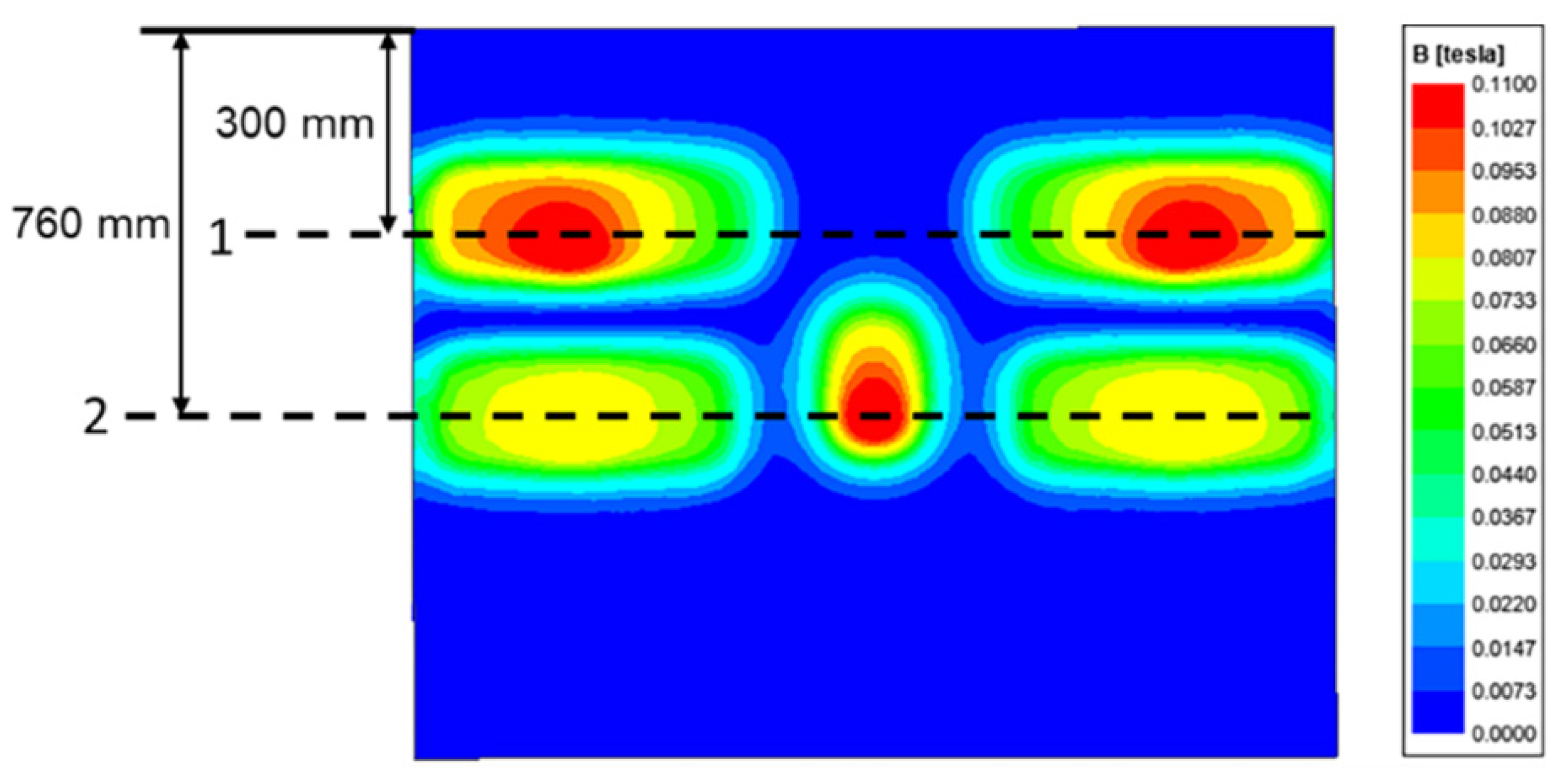
Figure 8.
Feature line values compared with measured data. (a) Feature line 1 and (b) feature line 2.
Figure 8.
Feature line values compared with measured data. (a) Feature line 1 and (b) feature line 2.

Figure 9.
Funnel mold electromagnetic field cloud map. (a) 300-200, (b) 800-600 and (c) 1100-800 A.
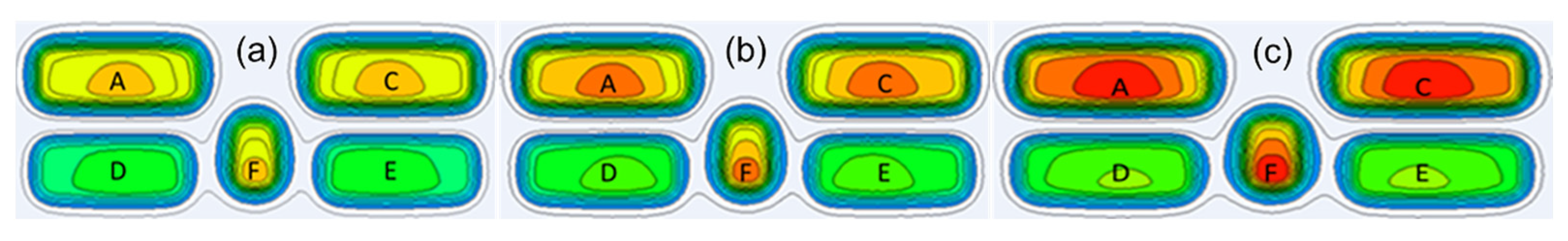
Figure 10.
Numerical simulation results of different currents. (a) Feature line 1 and (b) feature line 2.
Figure 10.
Numerical simulation results of different currents. (a) Feature line 1 and (b) feature line 2.
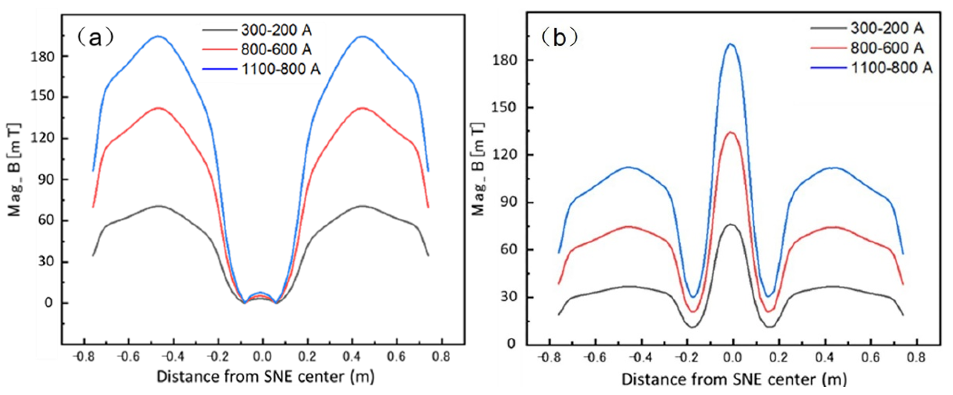
Figure 11.
Distribution of velocity and velocity vector on the centrally symmetric plane at different currents. (a) No EMBr, (b) 300-200, (c) 800-600 and (d) 1100-800 A.
Figure 11.
Distribution of velocity and velocity vector on the centrally symmetric plane at different currents. (a) No EMBr, (b) 300-200, (c) 800-600 and (d) 1100-800 A.
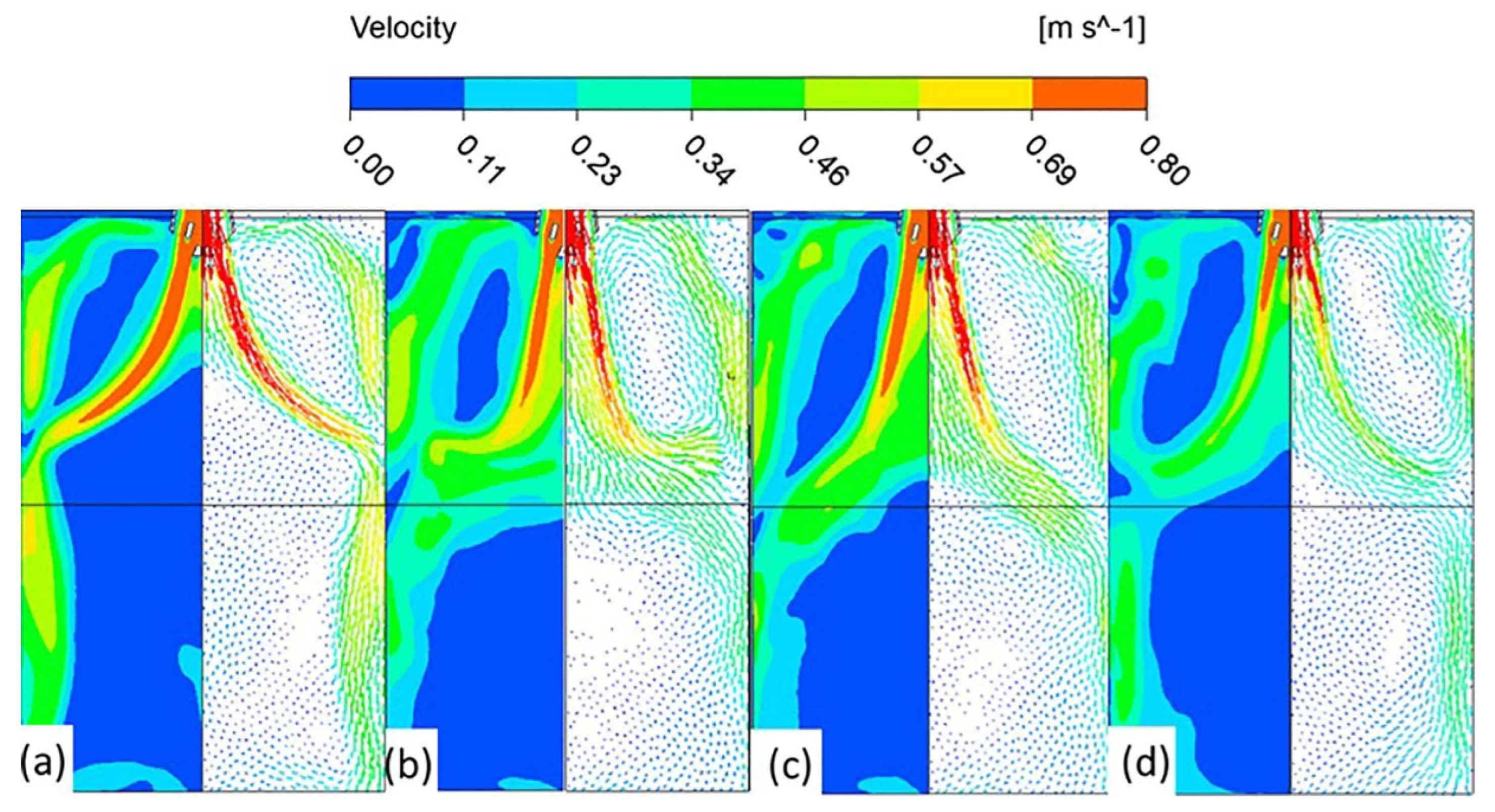
Figure 12.
Funnel mold narrow face velocity distribution and vector diagram. (a) No EMBr, (b) 300-200, (c) 800-600 and (d) 1100-800 A.
Figure 12.
Funnel mold narrow face velocity distribution and vector diagram. (a) No EMBr, (b) 300-200, (c) 800-600 and (d) 1100-800 A.

Figure 13.
Funnel mold surface velocity distribution.
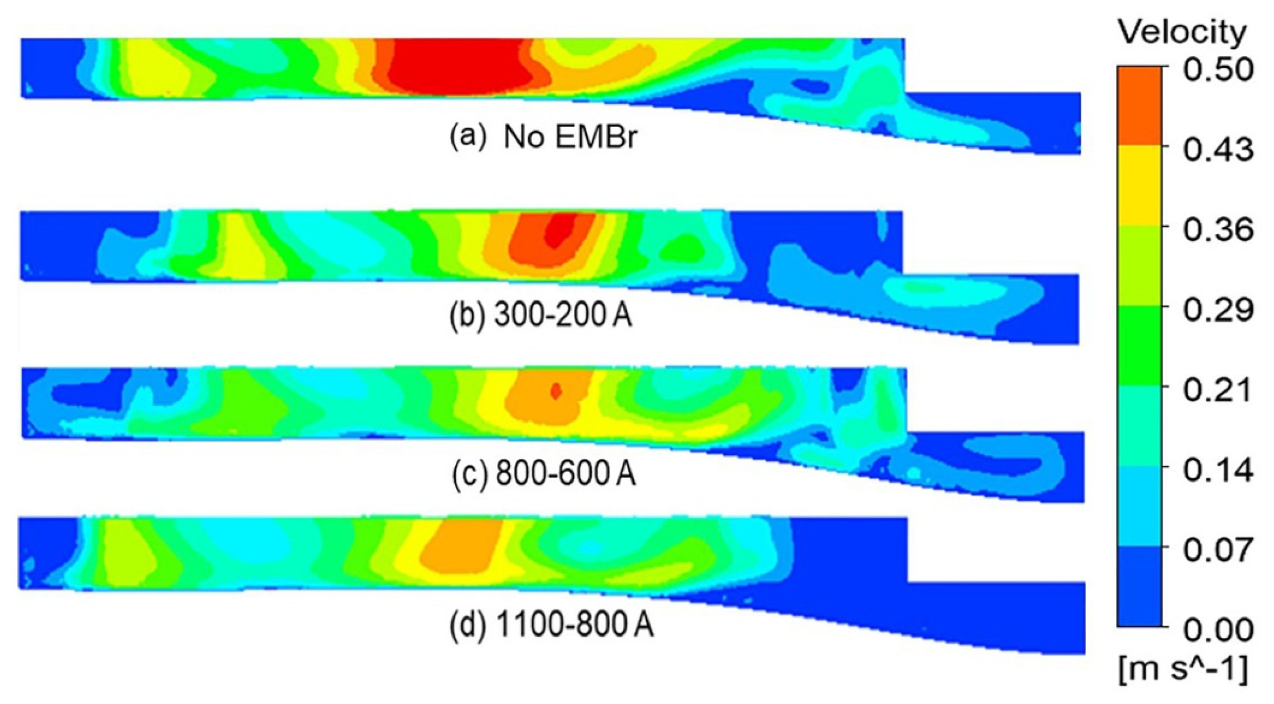
Figure 14.
Funnel mold surface velocity.
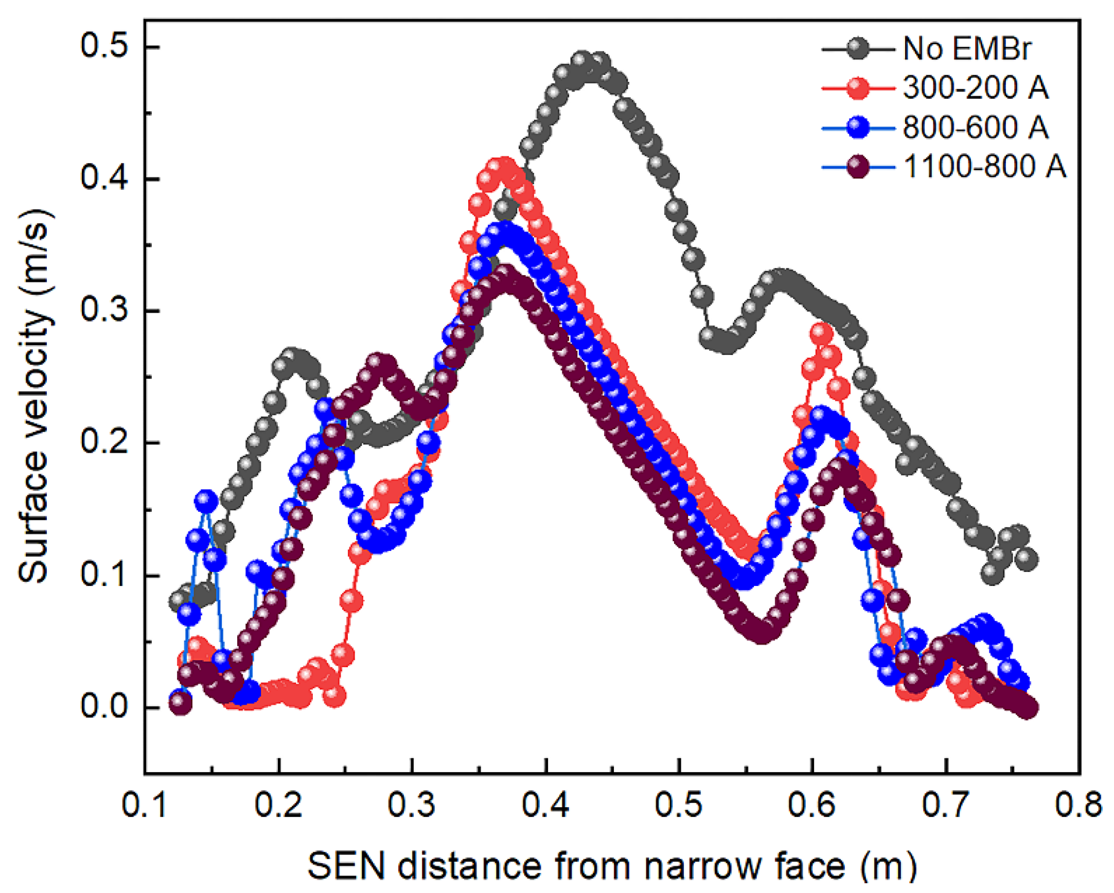
Figure 15.
The maximum value (absolute value) of liquid-level wave height at different times.
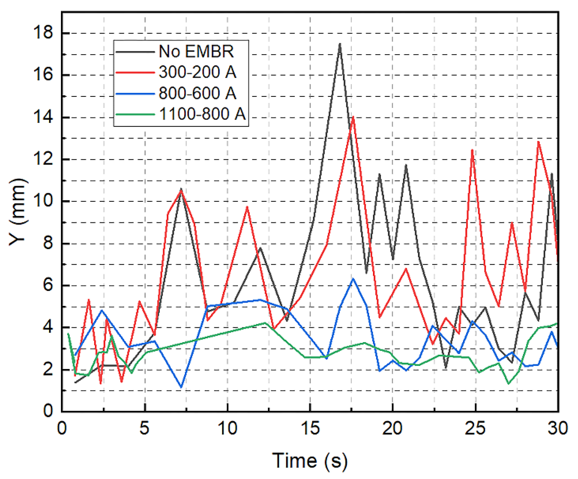
Figure 16.
Slag entrapment situation at liquid-level. (a) No EMBr, (b) 300-200, (c) 800-600 and (d) 1100-800 A.
Figure 16.
Slag entrapment situation at liquid-level. (a) No EMBr, (b) 300-200, (c) 800-600 and (d) 1100-800 A.

Figure 17.
Description of the nail board and position for dipping tests. (a) Nail board and (b) position for dipping tests.
Figure 17.
Description of the nail board and position for dipping tests. (a) Nail board and (b) position for dipping tests.
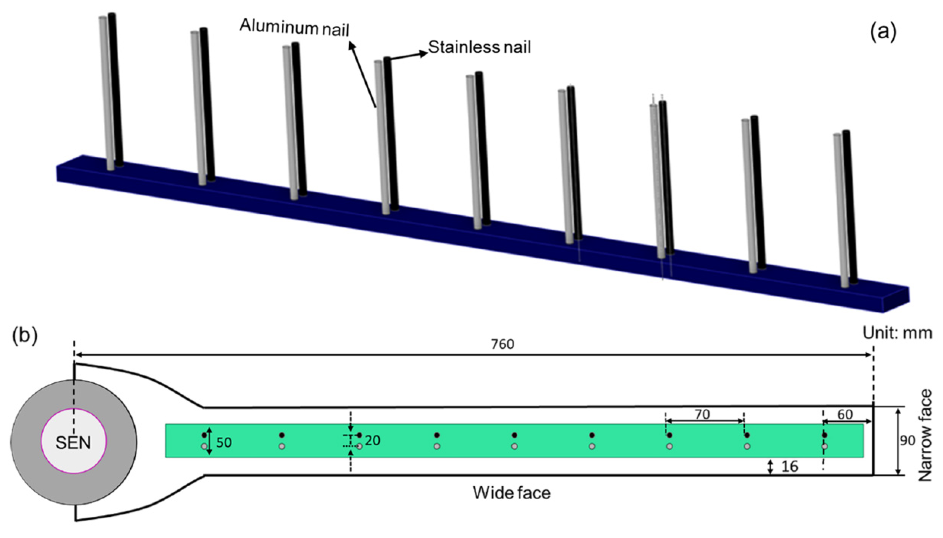
Figure 18.
Dipping tests. (a) Morphology of nails after dipping tests and (b) characteristic parameters of solidified steel lumps.
Figure 18.
Dipping tests. (a) Morphology of nails after dipping tests and (b) characteristic parameters of solidified steel lumps.

Figure 19.
Funnel mold surface velocity.

Figure 20.
Vector diagram of surface velocity on the meniscus.
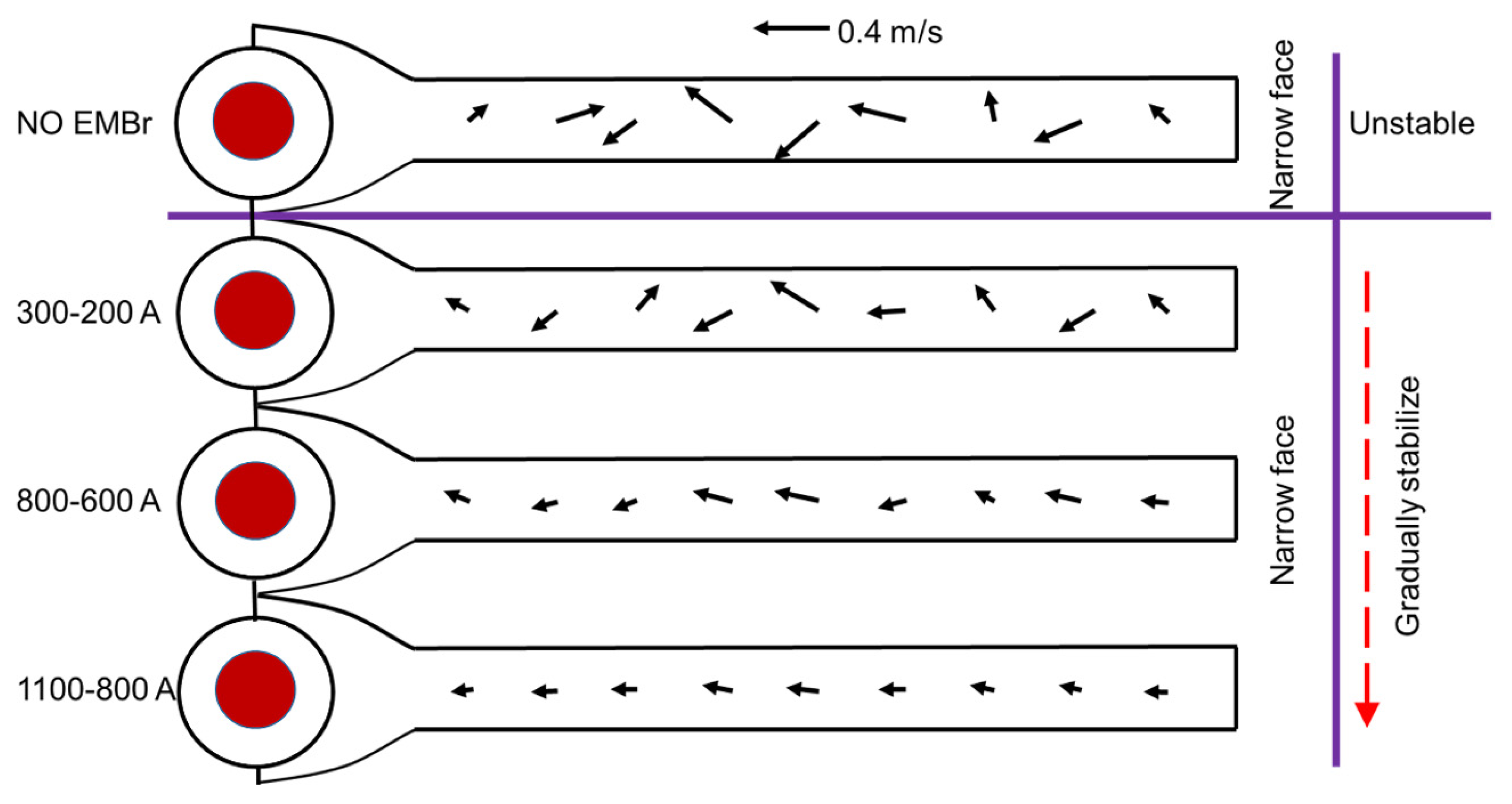
Figure 21.
Liquid-level waveform on the centerline of the wide face.
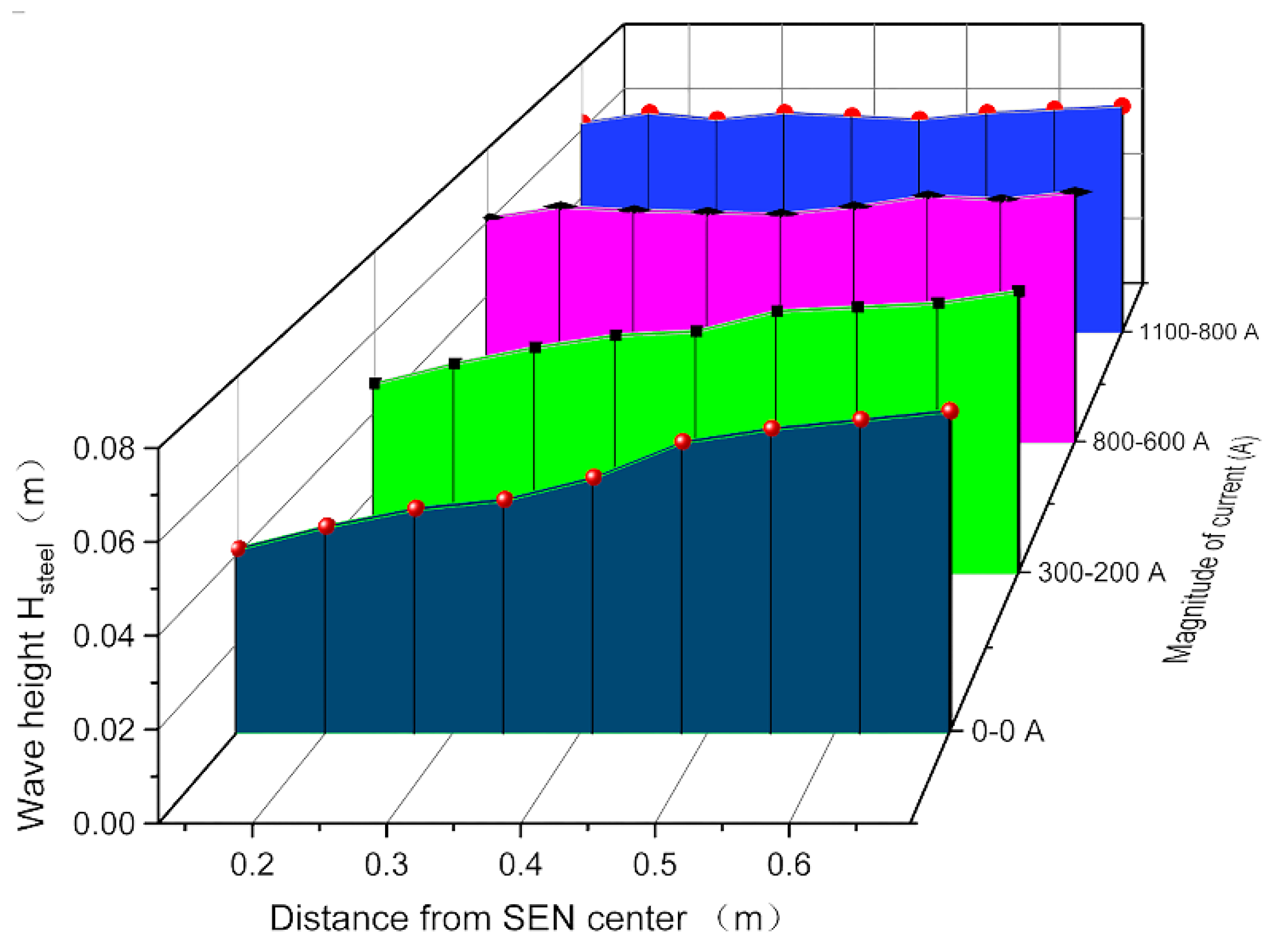
Figure 22.
The thickness of the liquid-slag layer. (a) No EMBr, (b) 300-200, (c) 800-600 and (d) 1100-800 A.
Figure 22.
The thickness of the liquid-slag layer. (a) No EMBr, (b) 300-200, (c) 800-600 and (d) 1100-800 A.


| Item | Value |
|---|---|
| FM width (mm) | 1520 |
| FM thickness (mm) | 90 |
| FM height (mm) | 1200 |
| SEN inlet diameter (mm) | 80 |
| SEN submergence depth (mm) | 160 |
| Casting speed (m/min) | 6 |
| Molten steel density (kg/m3) | 7020 |
| Molten steel viscosity (Pa·s) | 0.0064 |
| Slag/molten steel surface tension (N/m) | 1.3 |
| Liquid-slag density (kg/m3) | 2700 |
| Liquid-slag viscosity (Pa·s) | 0.18 |
| Core relative permeability | 4000 |
| Electrical conductivity of core (S/m) | 1.12 × 10⁷ |
| Distance from core to FM domain (mm) | 50 |
| Thickness of copper coil (mm) | 65 |
| Copper coil relative permeability | 1 |
| Electrical conductivity of molten steel (S/m) | 7.14 × 10⁵ |
| Air relative permeability | 1 |
| Electrical conductivity of air (S/m) | 1.0 × 10⁻⁵ |
Table 2.
Details of the current of each magnetic pole.
| Number | Magnetic Pole (A/C) Coil Current | Magnetic Pole (F/D/E) Coil Current |
|---|---|---|
| 1 | 300 A | 200 A |
| 2 | 800 A | 600 A |
| 3 | 1100 A | 800 A |
Disclaimer/Publisher’s Note: The statements, opinions and data contained in all publications are solely those of the individual author(s) and contributor(s) and not of MDPI and/or the editor(s). MDPI and/or the editor(s) disclaim responsibility for any injury to people or property resulting from any ideas, methods, instructions or products referred to in the content. |
© 2023 by the authors. Licensee MDPI, Basel, Switzerland. This article is an open access article distributed under the terms and conditions of the Creative Commons Attribution (CC BY) license (https://creativecommons.org/licenses/by/4.0/).
Share and Cite
MDPI and ACS Style
Zhang, L.; Xiao, P.; Wang, Y.; Zhang, C.; Zhu, L. Effect of EMBr on Flow in Slab Continuous Casting Mold and Industrial Experiment of Nail Dipping Measurement. Metals 2023, 13, 167. https://doi.org/10.3390/met13010167
AMA Style
Zhang L, Xiao P, Wang Y, Zhang C, Zhu L. Effect of EMBr on Flow in Slab Continuous Casting Mold and Industrial Experiment of Nail Dipping Measurement. Metals. 2023; 13(1):167. https://doi.org/10.3390/met13010167
Chicago/Turabian StyleZhang, Limin, Pengcheng Xiao, Yan Wang, Caijun Zhang, and Liguang Zhu. 2023. "Effect of EMBr on Flow in Slab Continuous Casting Mold and Industrial Experiment of Nail Dipping Measurement" Metals 13, no. 1: 167. https://doi.org/10.3390/met13010167
Note that from the first issue of 2016, this journal uses article numbers instead of page numbers. See further details here.