
Modeling the Evolution of Grain Texture during Solidification of Laser-Based Powder Bed Fusion Manufactured Alloy 625 Using a Cellular Automata Finite Element Model

Abstract
:1. Introduction
2. Materials and Methods
2.1. Finite Element Model
2.2. 2D Cellular Automata Model
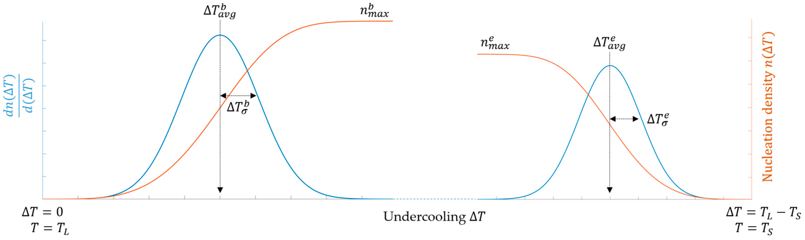
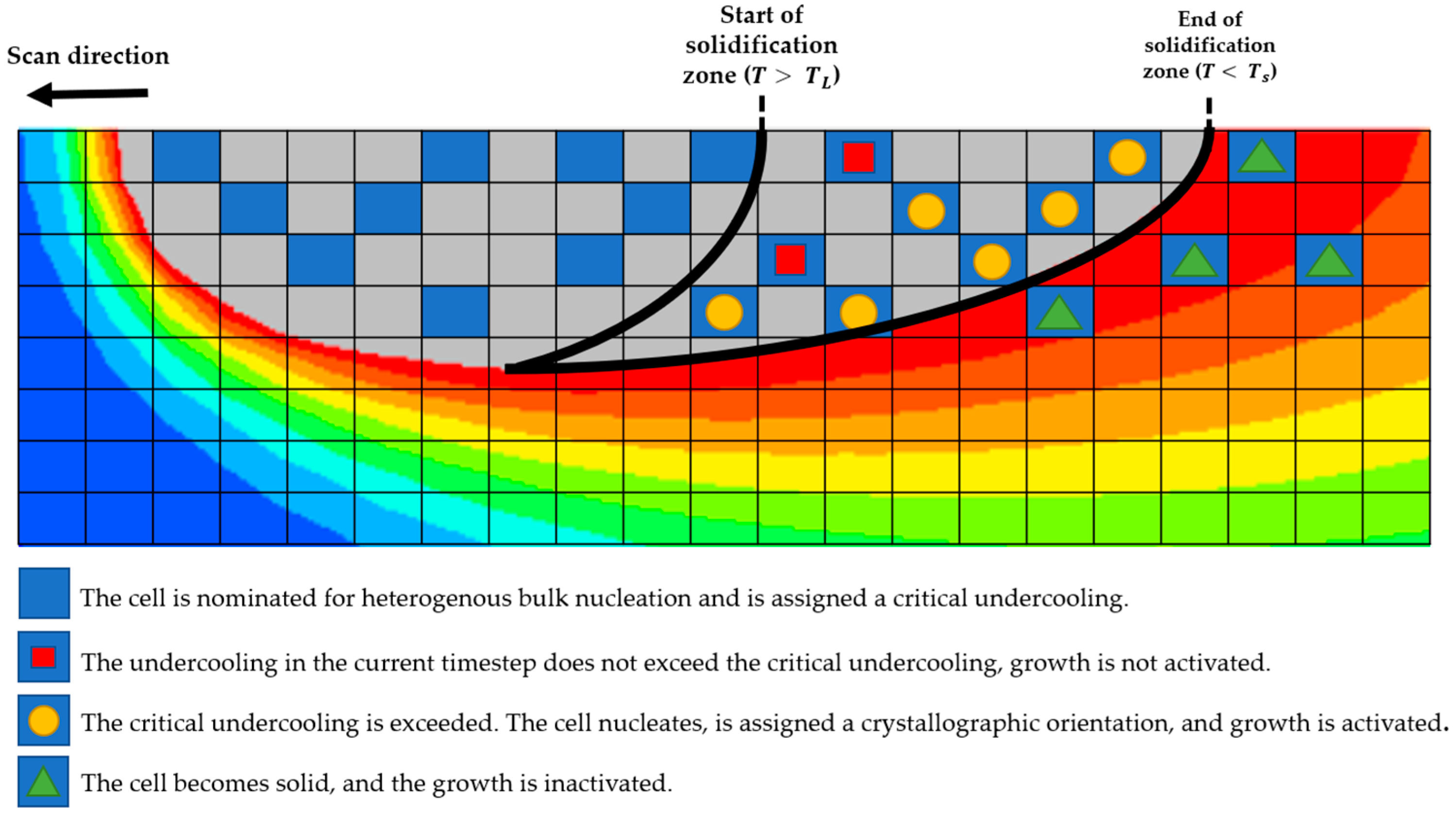
2.2.1. Nucleation
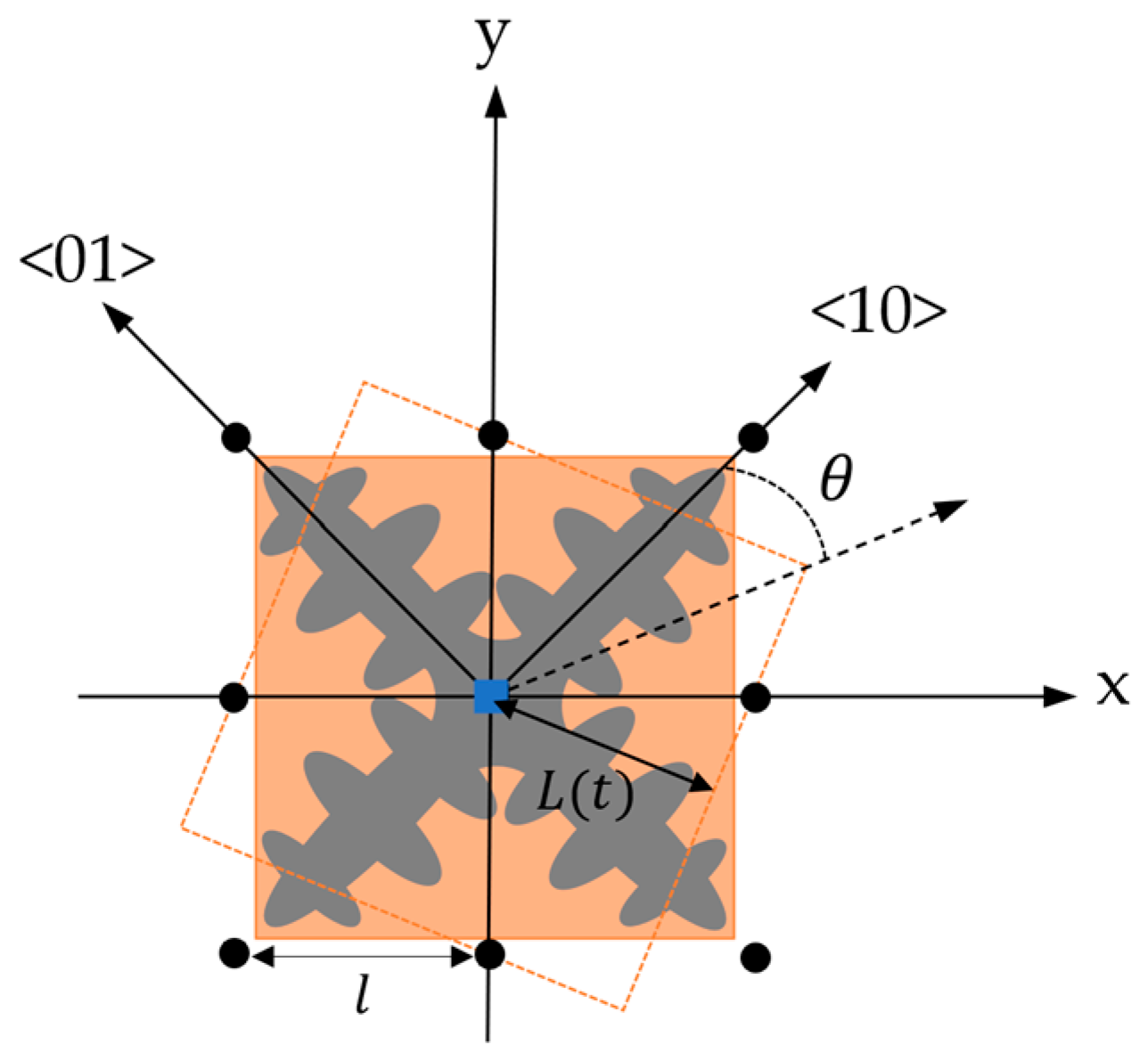
2.2.2. Grain Growth
3. Results and Discussion
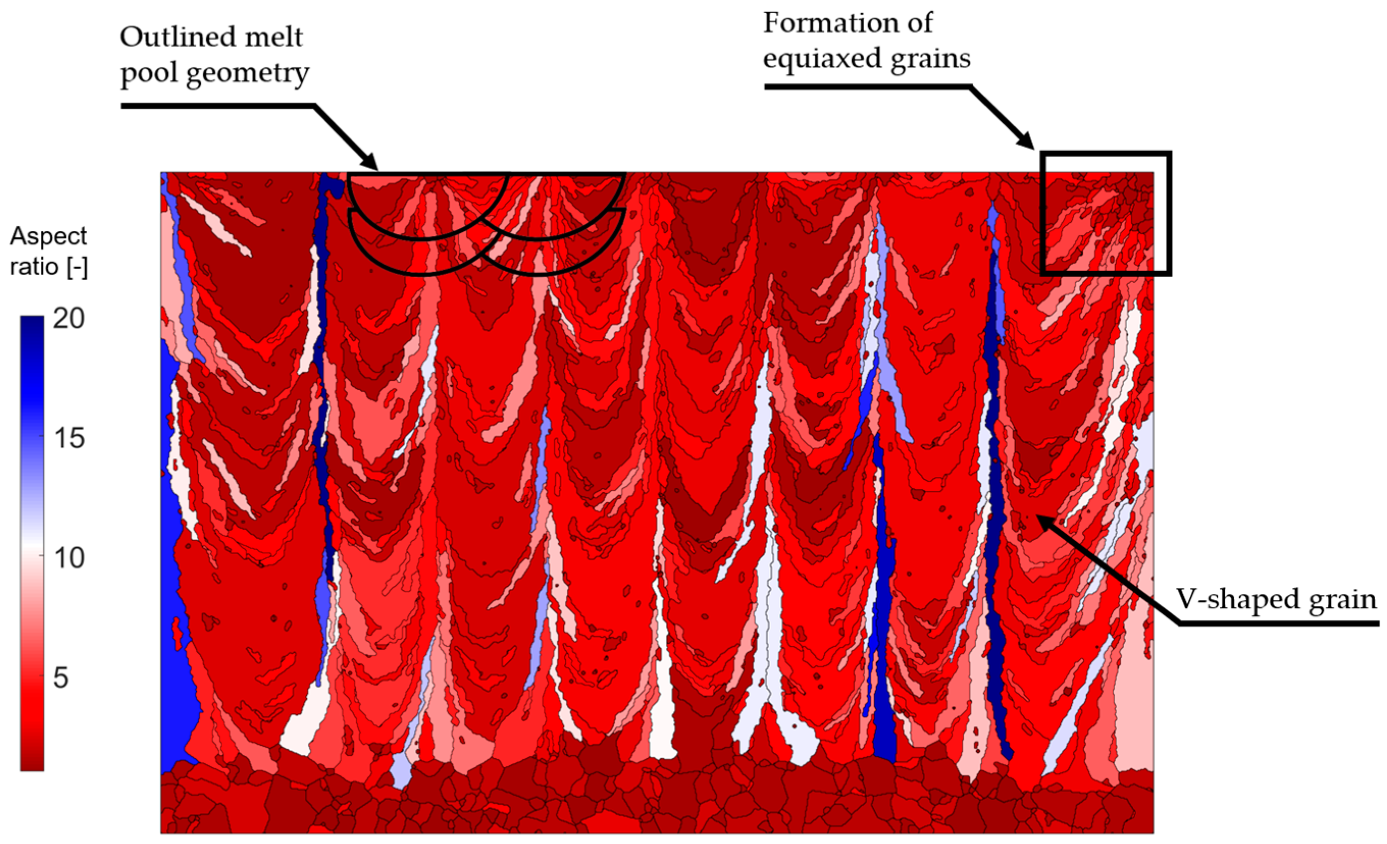
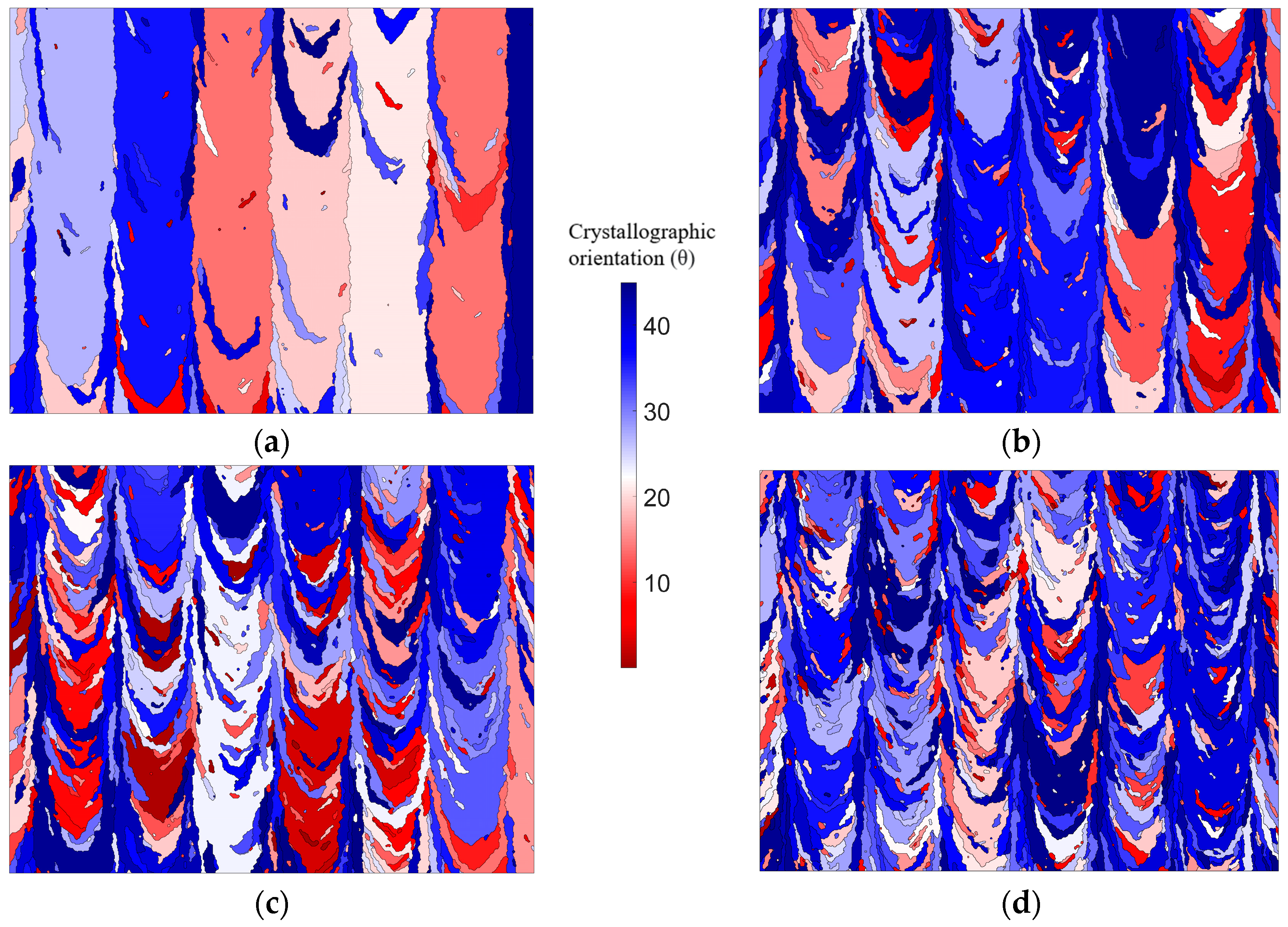
3.1. Characteristics of the As-Solidified Grain Texture
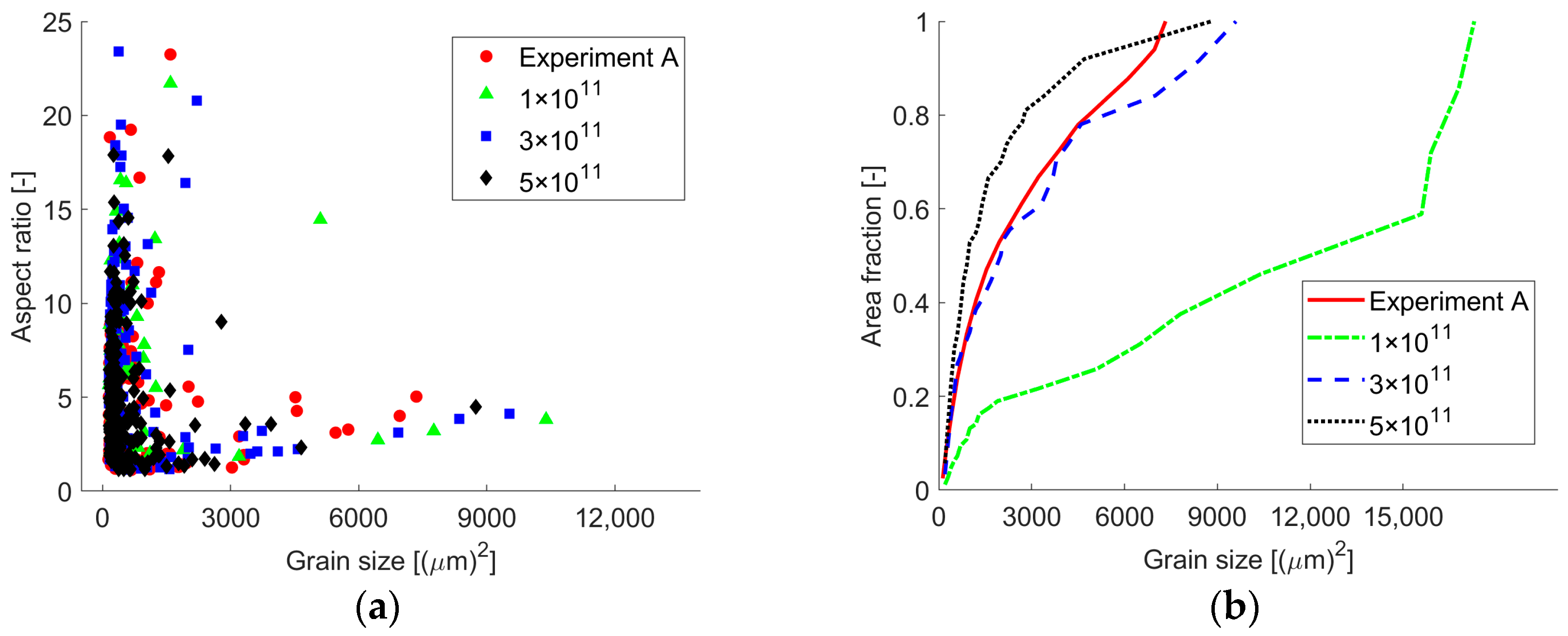
3.2. Influence on Grain Texture by Nucleation Density
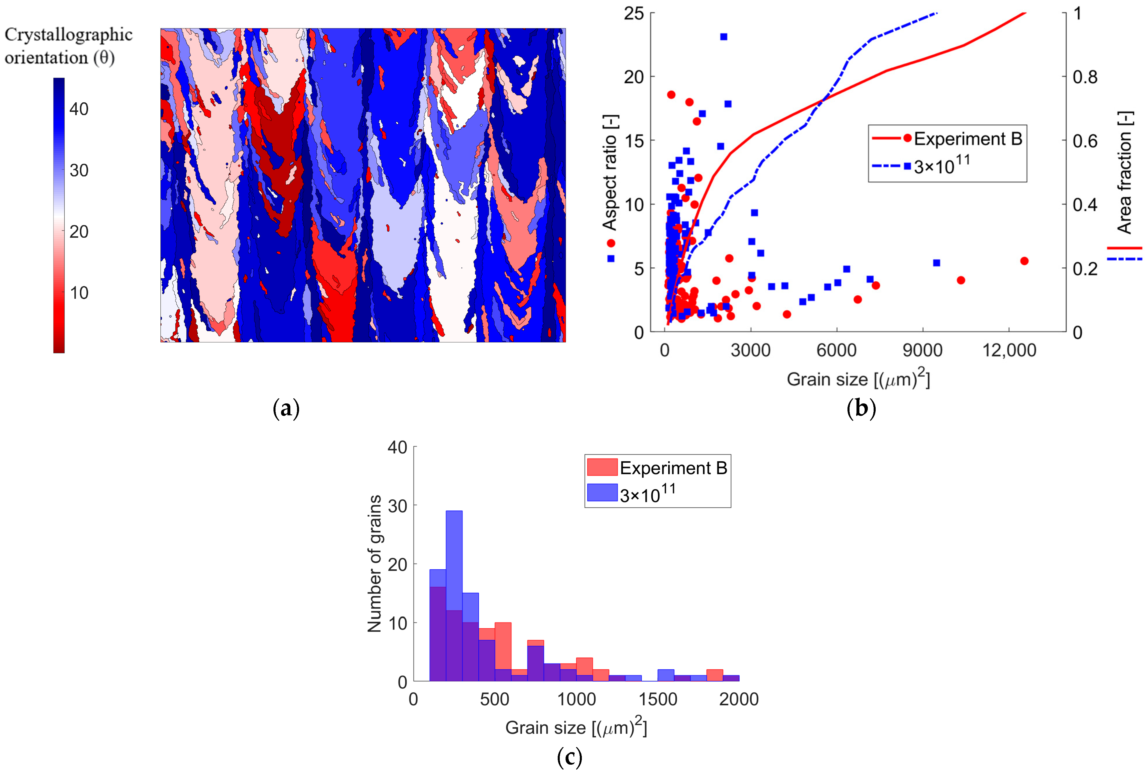
3.3. Influence on Grain Texture by Changed Process Parameters
4. Conclusions
Author Contributions
Funding
Data Availability Statement
Conflicts of Interest
References
- Ford, S.; Despeisse, M. Additive Manufacturing and Sustainability: An Exploratory Study of the Advantages and Challenges. J. Clean. Prod. 2016, 137, 1573–1587. [Google Scholar] [CrossRef]
- Petrovic, V.; Gonzalez, J.V.H.; Ferrando, O.J.; Delgado Gordillo, J.; Puchades, J.R.B.; Griñan, L.P. Additive Layered Manufacturing: Sectors of Industrial Application Shown through Case Studies. Int. J. Prod. Res. 2011, 49, 1061–1079. [Google Scholar] [CrossRef]
- Volpato, G.M.; Tetzlaff, U.; Fredel, M.C. A Comprehensive Literature Review on Laser Powder Bed Fusion of Inconel Superalloys. Addit. Manuf. 2022, 55, 102871. [Google Scholar] [CrossRef]
- Dinda, G.P.; Dasgupta, A.K.; Mazumder, J. Laser Aided Direct Metal Deposition of Inconel 625 Superalloy: Microstructural Evolution and Thermal Stability. Mater. Sci. Eng. A 2009, 509, 98–104. [Google Scholar] [CrossRef]
- Shankar, V.; Bhanu Sankara Rao, K.; Mannan, S.L. Microstructure and Mechanical Properties of Inconel 625 Superalloy. J. Nucl. Mater. 2001, 288, 222–232. [Google Scholar] [CrossRef]
- Yan, X.; Gao, S.; Chang, C.; Huang, J.; Khanlari, K.; Dong, D.; Ma, W.; Fenineche, N.; Liao, H.; Liu, M. Effect of Building Directions on the Surface Roughness, Microstructure, and Tribological Properties of Selective Laser Melted Inconel 625. J. Mater. Process. Technol. 2021, 288, 116878. [Google Scholar] [CrossRef]
- Li, C.; White, R.; Fang, X.Y.; Weaver, M.; Guo, Y.B. Microstructure Evolution Characteristics of Inconel 625 Alloy from Selective Laser Melting to Heat Treatment. Mater. Sci. Eng. A 2017, 705, 20–31. [Google Scholar] [CrossRef]
- Malmelöv, A.; Hassila, C.J.; Fisk, M.; Wiklund, U.; Lundbäck, A. Numerical Modeling and Synchrotron Diffraction Measurements of Residual Stresses in Laser Powder Bed Fusion Manufactured Alloy 625. Mater. Des. 2022, 216, 110548. [Google Scholar] [CrossRef]
- Kou, S. Welding Metallurgy; Wiley: Hoboken, NJ, USA, 2002. [Google Scholar]
- Andreau, O.; Koutiri, I.; Peyre, P.; Penot, J.D.; Saintier, N.; Pessard, E.; De Terris, T.; Dupuy, C.; Baudin, T. Texture Control of 316L Parts by Modulation of the Melt Pool Morphology in Selective Laser Melting. J. Mater. Process. Technol. 2019, 264, 21–31. [Google Scholar] [CrossRef]
- Flood, S.C.; Hunt, J.D. Columnar and Equiaxed Growth: II. Equiaxed Growth Ahead of a Columnar Front. J. Cryst. Growth 1987, 82, 552–560. [Google Scholar] [CrossRef]
- Rappaz, M.; Gandin, C.A. Probabilistic Modelling of Microstructure Formation in Solidification Processes. Acta Metall. Mater. 1993, 41, 345–360. [Google Scholar] [CrossRef]
- Körner, C.; Markl, M.; Koepf, J.A. Modeling and Simulation of Microstructure Evolution for Additive Manufacturing of Metals: A Critical Review. Metall. Mater. Trans. A 2020, 51, 4970–4983. [Google Scholar] [CrossRef]
- Kurz, W.; Rappaz, M.; Trivedi, R. Progress in Modelling Solidification Microstructures in Metals and Alloys. Part II: Dendrites from 2001 to 2018. Int. Mater. Rev. 2020, 66, 30–76. [Google Scholar] [CrossRef]
- Gong, X.; Chou, K. Phase-Field Modeling of Microstructure Evolution in Electron Beam Additive Manufacturing. JOM 2015, 67, 1176–1182. [Google Scholar] [CrossRef]
- Rodgers, T.M.; Madison, J.D.; Tikare, V. Simulation of Metal Additive Manufacturing Microstructures Using Kinetic Monte Carlo. Comput. Mater. Sci. 2017, 135, 78–89. [Google Scholar] [CrossRef]
- Gandin, C.A.; Rappaz, M. A 3D Cellular Automaton Algorithm for the Prediction of Dendritic Grain Growth. Acta Mater. 1997, 45, 2187–2195. [Google Scholar] [CrossRef]
- Gandin, C.A.; Rappaz, M. A Coupled Finite Element-Cellular Automaton Model for the Prediction of Dendritic Grain Structures in Solidification Processes. Acta Metall. Mater. 1994, 42, 2233–2246. [Google Scholar] [CrossRef]
- Dezfoli, A.R.A.; Lo, Y.L.; Raza, M.M. Prediction of Epitaxial Grain Growth in Single-Track Laser Melting of IN718 Using Integrated Finite Element and Cellular Automaton Approach. Materials 2021, 14, 5202. [Google Scholar] [CrossRef]
- Rai, A.; Markl, M.; Körner, C. A Coupled Cellular Automaton–Lattice Boltzmann Model for Grain Structure Simulation during Additive Manufacturing. Comput. Mater. Sci. 2016, 124, 37–48. [Google Scholar] [CrossRef]
- Koepf, J.A.; Soldner, D.; Ramsperger, M.; Mergheim, J.; Markl, M.; Körner, C. Numerical Microstructure Prediction by a Coupled Finite Element Cellular Automaton Model for Selective Electron Beam Melting. Comput. Mater. Sci. 2019, 162, 148–155. [Google Scholar] [CrossRef]
- Teferra, K.; Rowenhorst, D.J. Optimizing the Cellular Automata Finite Element Model for Additive Manufacturing to Simulate Large Microstructures. Acta Mater. 2021, 213, 116930. [Google Scholar] [CrossRef]
- Isoltermics, Nicrofer6020 HMo—Alloy 625. Available online: https://www.isolthermics.com.au/metals/pdfs/common-tech/Alloy%20625%206020hMo.pdf (accessed on 18 August 2023).
- Special Metals, Inconel Alloy 625. Available online: https://www.specialmetals.com/documents/technical-bulletins/inconel/inconel-alloy-625.pdf (accessed on 18 August 2023).
- Denlinger, E.R.; Michaleris, P. Effect of Stress Relaxation on Distortion in Additive Manufacturing Process Modeling. Addit. Manuf. 2016, 12, 51–59. [Google Scholar] [CrossRef]
- Wei, L.C.; Ehrlich, L.E.; Powell-Palm, M.J.; Montgomery, C.; Beuth, J.; Malen, J.A. Thermal Conductivity of Metal Powders for Powder Bed Additive Manufacturing. Addit. Manuf. 2018, 21, 201–208. [Google Scholar] [CrossRef]
- Tinoco, J.; Fredriksson, H. Solidification of a Modified Inconel 625 Alloy under Different Cooling Rates. High Temp. Mater. Process. 2004, 23, 13–24. [Google Scholar] [CrossRef]
- Goldak, J.; Chakravarti, A.; Bibby, M. A New Finite Element Model for Welding Heat Sources. Metall. Trans. B 1984, 15, 299–305. [Google Scholar] [CrossRef]
- Lindgren, L.-E. Computational Welding Mechanics: Thermomechanical and Microstructural Simulations; Woodhead Publishing Ltd.: Cambridge, UK, 2007; ISBN 9781845692216. [Google Scholar]
- Mohebbi, M.S.; Ploshikhin, V. Implementation of Nucleation in Cellular Automaton Simulation of Microstructural Evolution during Additive Manufacturing of Al Alloys. Addit. Manuf. 2020, 36, 101726. [Google Scholar] [CrossRef]
- Lipton, J.; Glicksman, M.E.; Kurz, W. Dendritic Growth into Undercooled Alloy Metals. Mater. Sci. Eng. 1984, 65, 57–63. [Google Scholar] [CrossRef]
- Kurz, W.; Giovanola, B.; Trivedi, R. Theory of Microstructural Development during Rapid Solidification. Acta Metall. 1986, 34, 823–830. [Google Scholar] [CrossRef]
- Zinoviev, A.; Zinovieva, O.; Ploshikhin, V.; Romanova, V.; Balokhonov, R. Evolution of Grain Structure during Laser Additive Manufacturing. Simulation by a Cellular Automata Method. Mater. Des. 2016, 106, 321–329. [Google Scholar] [CrossRef]
- Tsai, D.C.; Hwang, W.S. A Three Dimensional Cellular Automaton Model for the Prediction of Solidification Morphologies of Brass Alloy by Horizontal Continuous Casting and Its Experimental Verification. Mater. Trans. 2011, 52, 787–794. [Google Scholar] [CrossRef]
- Wang, W.; Lee, P.D.; McLean, M. A Model of Solidification Microstructures in Nickel-Based Superalloys: Predicting Primary Dendrite Spacing Selection. Acta Mater. 2003, 51, 2971–2987. [Google Scholar] [CrossRef]
- Yang, M.; Wang, L.; Yan, W. Phase-Field Modeling of Grain Evolutions in Additive Manufacturing from Nucleation, Growth, to Coarsening. NPJ Comput. Mater. 2021, 7, 56. [Google Scholar] [CrossRef]
- Wang, L.Y.; Wang, Y.C.; Zhou, Z.J.; Wan, H.Y.; Li, C.P.; Chen, G.F.; Zhang, G.P. Small Punch Creep Performance of Heterogeneous Microstructure Dominated Inconel 718 Fabricated by Selective Laser Melting. Mater. Des. 2020, 195, 109042. [Google Scholar] [CrossRef]


| Property | Value | Unit |
|---|---|---|
| [8] | 100 | W |
| [8] | 1200 | mm/s |
| [8] | 160 | W |
| [8] | 1400 | mm/s |
| 0.34 | - | |
| e | 35 | |
| 20 | ||
| 15 | ||
| 25 | ||
| 500 | ||
| Density [24] | kg/m3 |
| Property | Value | Unit |
|---|---|---|
| [35] | m2/s | |
| [35] | −10.9 | K/wt% |
| [35] | 0.48 | - |
| [35] | m | |
| [35] | 4.85 | wt% |
| - | ||
| - | ||
| - |
| Cell State | Condition | Effect in CA Model |
|---|---|---|
| Liquid | . | that must be exceeded for a nucleus to form. |
| Nucleated | . | . |
| Growing | . | to captured cells |
| Solid | . | , does not grow, and cannot be captured by other cells. |
Disclaimer/Publisher’s Note: The statements, opinions and data contained in all publications are solely those of the individual author(s) and contributor(s) and not of MDPI and/or the editor(s). MDPI and/or the editor(s) disclaim responsibility for any injury to people or property resulting from any ideas, methods, instructions or products referred to in the content. |
© 2023 by the authors. Licensee MDPI, Basel, Switzerland. This article is an open access article distributed under the terms and conditions of the Creative Commons Attribution (CC BY) license (https://creativecommons.org/licenses/by/4.0/).
Share and Cite
Andersson, C.; Lundbäck, A. Modeling the Evolution of Grain Texture during Solidification of Laser-Based Powder Bed Fusion Manufactured Alloy 625 Using a Cellular Automata Finite Element Model. Metals 2023, 13, 1846. https://doi.org/10.3390/met13111846
Andersson C, Lundbäck A. Modeling the Evolution of Grain Texture during Solidification of Laser-Based Powder Bed Fusion Manufactured Alloy 625 Using a Cellular Automata Finite Element Model. Metals. 2023; 13(11):1846. https://doi.org/10.3390/met13111846
Chicago/Turabian StyleAndersson, Carl, and Andreas Lundbäck. 2023. "Modeling the Evolution of Grain Texture during Solidification of Laser-Based Powder Bed Fusion Manufactured Alloy 625 Using a Cellular Automata Finite Element Model" Metals 13, no. 11: 1846. https://doi.org/10.3390/met13111846