
Parent Grain Reconstruction in an Additive Manufactured Titanium Alloy

Gatan + EDAX, Pleasanton, 94588 CA, USA
*
Author to whom correspondence should be addressed.
Metals 2024, 14(1), 51; https://doi.org/10.3390/met14010051
Submission received: 30 October 2023
/
Revised: 15 December 2023
/
Accepted: 18 December 2023
/
Published: 30 December 2023
(This article belongs to the Section Additive Manufacturing)
Abstract
:Electron backscatter diffraction (EBSD) is an excellent tool for characterizing the crystallographic orientation aspects of the microstructure of polycrystalline material. In some additively manufactured materials, the material may undergo a phase transformation during the forming process. Although EBSD can only characterize the final microstructure, neighbor information from orientation mapping allows the microstructure before the phase transformation to be reconstructed, provided that the parent–child orientation relationship is known. An investigation of the effectiveness of the reconstruction algorithms for capturing the grain size as well as orientation gradients is undertaken with a focus on additively manufactured Ti-alloy. The EBSD results, coupled with reconstruction algorithms, reveal information on the prior grain size as well as the plastic flow of the material.
1. Introduction
Electron backscatter diffraction (EBSD) in the scanning electron microscope (SEM) is a widely used microstructural characterization tool. Although EBSD can only determine the microstructure present at the time of characterization, neighbor information from mapping enables the reconstruction of a pre-transformation phase if the parent–child orientation relationship is known. Several researchers have developed algorithms for reconstructing the microstructure prior to the phase transformation [1,2,3,4,5,6,7]. The algorithms have been developed for EBSD acquired using regular square grids. We have implemented the probabilistic reconstruction approach outlined by Ranger et al. [4] for data collected on a hexagonal grid into the EDAX OIM Analysis™ post-processing software package. This paper reports, first, on the effectiveness of the implemented algorithm for parent grain reconstruction and, second, on the effect of parameters that can be varied in applying the algorithm. The experiments reported will focus primarily on EBSD results obtained from a Ti alloy (Ti6Al4V) formed by powder bed additive manufacturing (AM).
2. Materials and Methods
2.1. EBSD Measurements
EBSD measurements were acquired from two samples. First, an additively manufactured sample of Ti6Al4V and second, from a sample of cobalt. All EBSD scans were performed using standard Hough transform-based indexing [8]. All samples examined in this study were mechanically polished with a final polish of colloidal silica in conjunction with a vibratory polisher.
The Ti6Al4V sample is for medical implant material formed by powder bed AM. After the AM process, the material underwent hot isostatic pressing (HIP). EBSD measurements were collected using an EDAX (Mahwah, NJ, USA) Hikari Super EBSD detector on a FEI (Hillsboro, OR, USA) XL-30 FEG-SEM at an accelerating voltage of 20 kV. The sample was tilted to 78.7° from horizontal, and the working distance was 12.5 mm. EBSD orientation mapping scans were performed at two different magnifications. The first, using a step size of 0.2 μm on a 225 μm wide × 179 μm tall hexagonal grid (1.16 million points), and the second, using a 0.6 μm step size on a 900 μm × 716 μm hexagonal grid (2.07 million points). The phase distribution for the lower magnification scan was 97.3% transformed α and 2.6% prior β. The higher magnification sample was measured to be 96.9% α and 3.1% β. The slightly larger fraction of β in the higher magnification sample is likely due to the smaller step size. The retained β grains were relatively small and thus could be missed by the larger step size in the lower magnification scan. This is reflected in the observation that the number of data points per β grain in the lower magnification scan was 1.6, versus 3.7 in the higher magnification scan.
Energy dispersive spectroscopy (EDS) data were also collected simultaneously with the EBSD measurements, allowing the spatial distribution of the chemical composition to be correlated with each phase, as determined by EBSD. The EDS and EBSD maps showed some correlation, with higher aluminum and vanadium content in the β phase. This was confirmed by simple averaging of the EDS counts in each phase, as shown in Table 1.
The cobalt measurements were obtained using an EDAX (Mahwah, NJ, Utah) Hikari EBSD detector on a FEI (Hillsboro) XL-30 FEG-SEM equipped with a TSL Solutions (Sagamihara, Japan) KK in-situ heating stage at an accelerating voltage of 20 kV. The sample was tilted to 70° from horizontal, and the working distance was 15 mm. All the scans in the in-situ experiment reported here were collected on 90 μm × 87 μm hexagonal grids with 0.5 μm spacing, resulting in 36.4 thousand-point scans. The same area was repeatedly scanned at temperatures ranging from room temperature to 500 °C, as measured at the specimen surface, and back to room temperature [9].
With the exception of the low magnification scan on the AM Ti sample, the scan areas presented are relatively small in area and not intended to provide a representative picture of the microstructure but to allow the details of the reconstruction to be examined. Larger scan areas were performed on the cobalt in-situ measurements, and the same trends were found in these measurements as in the detailed scans presented.
No cleanup procedures were applied to any of the EBSD data used in this study. The orientation maps presented show the crystal direction aligned with a specified sample direction. Such maps are generally called inverse pole figure (IPF) maps. The sample direction for the IPF maps is the sample normal, unless specified otherwise. The sample normal IPFs are denoted by IPF||ND for brevity. The color scheme used for all IPF maps is given in Figure 1a.
2.2. Reconstruction Methodology
The parent microstructure algorithm implementation applied to the EBSD measurements was that provided in version 9 of EDAX OIM Analysis™. This implementation follows the probabilistic reconstruction approach outlined by Ranger et al. [4], expanded to provide reconstruction of EBSD data collected on both square and hexagonal grids.
As noted in the Introduction, several methods of parent microstructure reconstruction have been reported in the literature. These can be broken down into two groups: (1) those using a variant grouping method [1,2,3,4,5], and (2) those using an adaptation of the computer vision graph-cut algorithm [6,7]. As the method used in this study is part of group (1), we provide a short summary of the technique. The reader is referred to the individual papers for more detail. A list of candidate parents can be constructed for each child variant based on crystallographically symmetric equivalents of a specified orientation relationship (OR). The OR may be specified or extracted from the EBSD data directly. The most probable parent is found by comparing the lists of candidate parents between neighboring variants and searching for common candidate–parent orientations. In some cases, there may be some ambiguity, and the different algorithms resolve the ambiguity in different manners. The orientation within the variants may also vary slightly, and handling this orientation variation differs between the different algorithms. This can be handled through refinement of the OR in different ways or at different stages in the process. Huang et al. [5] refine the OR prior to the variant grouping, Miyamoto et al. [2] refine the OR as part of the assignment process using a sliding window. For the method used in this study, the OR is refined after reconstruction (see Section 3.3). Germain et al. [3] add an additional topological refinement, resulting in less jagged grain boundaries. Several of these algorithms have been applied to an EBSD dataset obtained from a low-alloy steel rolled-sheet sample with fully transformed ferrite (body-centered cubic—bcc) microstructure to obtain a reconstructed parent austenite (face-centered cubic—fcc) microstructure. The EBSD dataset is the same as that used by Ranger et al. [4] and was obtained on a transverse section of the rolled sheet. The specified OR used in the reconstructions is the Nishiyama–Wasserman OR:
The results show good agreement in the parent grain orientations and shapes, with some variation in the smaller grains, particularly in the immediate vicinity of the grain boundaries. It is assumed that additional adjustments to the different parameters used in these reconstruction algorithms by experts in their use could bring them to closer agreement.
3. Results and Discussion
3.1. Reconstruction Fidelity
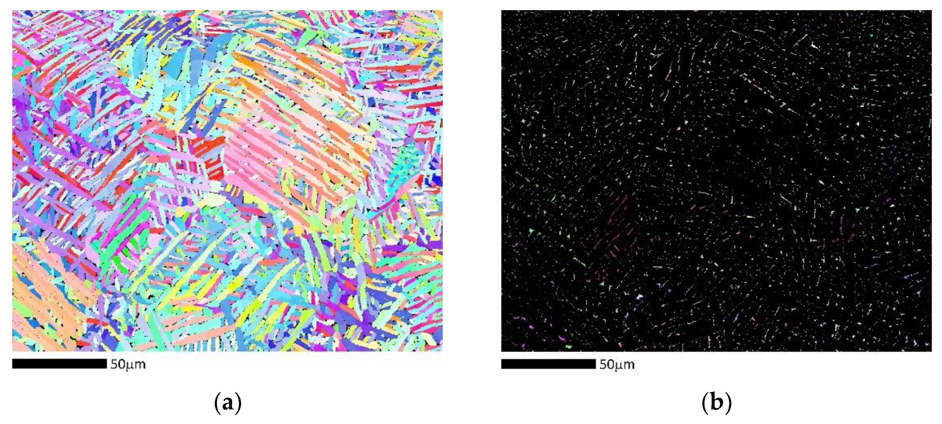
The EBSD results obtained from the Ti alloy showed the microstructure after AM to be composed primarily of the hexagonal α phase. Figure 2a shows an orientation map (i.e., the inverse pole figure or IPF map, which shows the crystal direction aligned with the normal sample via the color scheme shown in the accompanying color triangles) with a microstructure characteristic of a material having undergone a phase transformation where grains in the parent phase (body-centered cubic β phase) have transformed into different crystallographic variants of the child phase (hexagonal α) forming a lamellar, or Widmanstätten, structure. Approximately 3% of the retained β phase was detected in the EBSD measurements, and their orientations are shown in Figure 2b. A visual inspection of Figure 2b provides a rough approximation of the grains in the prior β structure.
The dilation approach [10], typically used to connect misindexed and non-indexed points to well-indexed points, can be applied to the retained β phase to provide a coarse reconstruction of the parent microstructure. Pixels of the α phase are essentially set to non-indexed pixels. Then, grains of the retained β phase are dilated iteratively until they meet other dilating retained β grains, and the scan area is completely filled with β grains. Results are shown in Figure 3a. Similarly, a Delaunay triangulation of the retained β grains [11,12] can also provide a coarse estimate of the parent β phase microstructure, as shown in Figure 3b. Both methods were performed with points indexed as β with a confidence index (CI) [13] greater than 0.2. Figure 3c is the prior β phase microstructure, as predicted by the implemented reconstruction algorithm. The reconstruction in Figure 3c assumes the following orientation relationship (OR) between the parent β phase and the child α phase.
A comparison of the figures confirms, at a rudimentary level, that the reconstruction algorithm captures the prior β microstructure.
To ensure that the reconstruction results were not unduly governed by the retained β phase in the EBSD measurements, the same reconstruction was performed after setting each of the retained β phase measurements to non-indexed points. A comparison of the results shown in Figure 3c (reconstructed, including the retained β points) and Figure 4 (reconstructed, excluding the retained β points) shows only subtle differences between the reconstructions performed with and without the retained β phase. This confirms that nearly the same reconstructed microstructure is obtained with or without any pre-transformation phase in the as-measured microstructure.
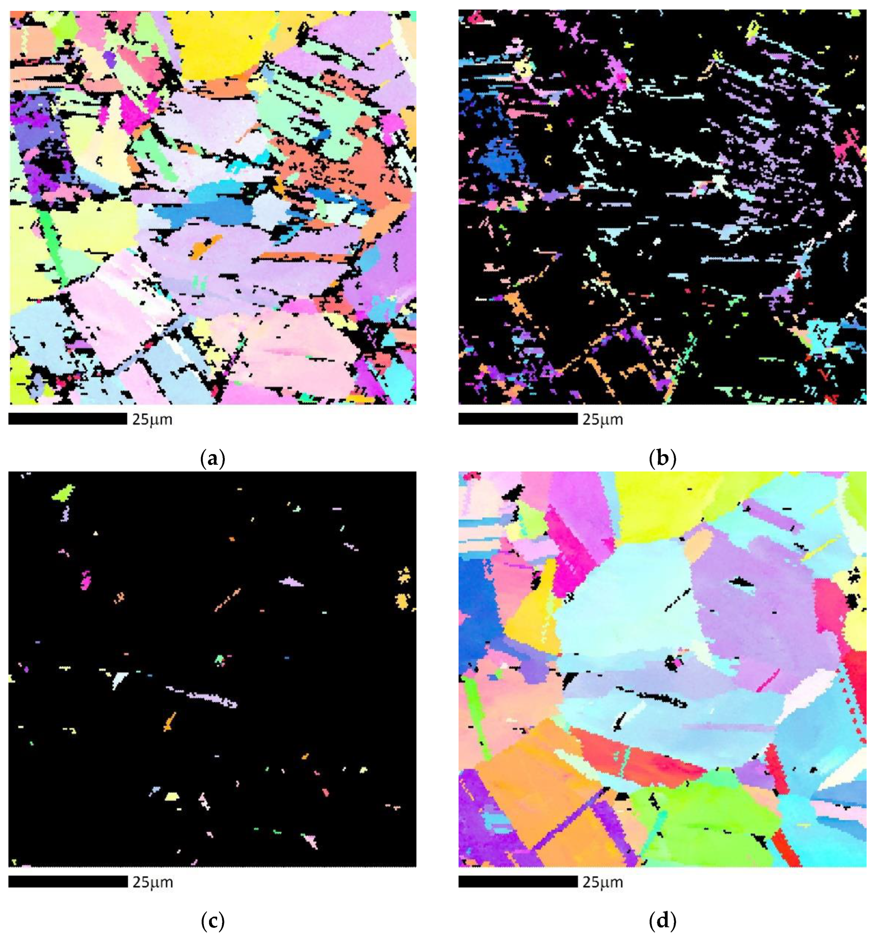
Physical methods used to directly confirm the validity of the reconstruction include etchants which decorate the prior parent phase grains [14] as well as in-situ experiments. We turn to in-situ EBSD measurements of cobalt to gain additional confirmation of the implemented algorithm. Cobalt has a transition temperature of 422 °C between the high-temperature face-centered cubic β phase and the low-temperature hexagonal α phase. Figure 5 shows the orientation maps for measurements made at room temperature and at 500 °C. It should be noted that room-temperature EBSD maps obtained before and after heating were nearly identical, even after several cycles.
The orientation relationship used in the cobalt prior parent reconstruction was:
The orientation relationship was confirmed from individual EBSD patterns captured at neighboring points in the partially transformed sample, as shown in Figure 6. Note that the (0001) basal plane highlighted in the EBSD pattern for the low-temperature hexagonal α phase aligns with the (111) normal plane highlighted in the EBSD pattern for the high-temperature cubic β phase.
Figure 7 shows the high-temperature microstructure reconstructed from the low-temperature EBSD measurements.
Although the sampling area is small, several statistical comparison metrics were checked to see how well the reconstructed microstructure matched the room-temperature result. The area fraction grain size distribution exhibited an average difference of 1.5%, an average difference of 0.6% in the disorientation angle distribution (20 bins ranging from 5° to 65°), and a difference of 0.36 times random in the respective orientation distribution functions (ODFs), with maxima of 34 and 36 times random. The ODFs were calculated using generalized spherical harmonics to a series expansion order of 16 on a 5° × 5° × 5° grid in Euler angle space.
3.2. Sampling Resolution
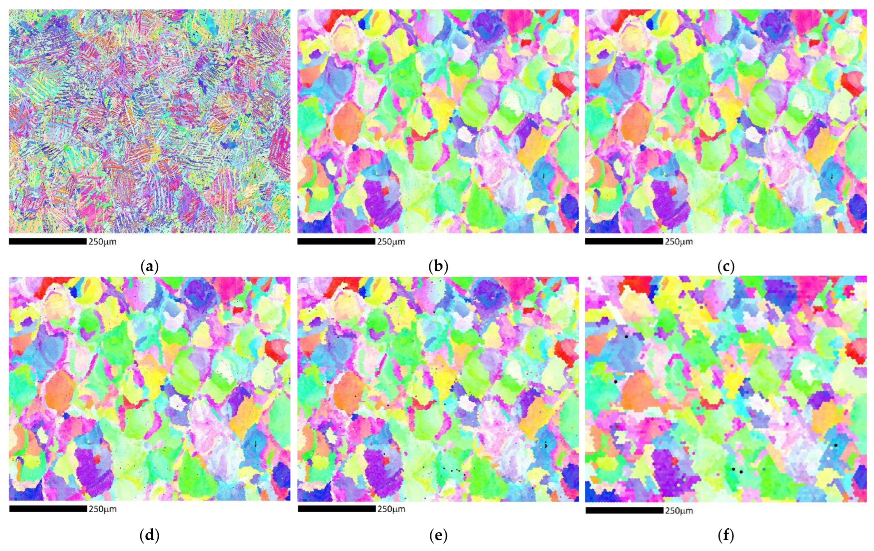
The examples shown have all had a good density of orientation measurements relative to the sampling area. However, the reconstruction does well, even with sparser sampling. A lower-magnification dataset from the AM Ti alloy was used to quantify this. The dataset contained just over two million EBSD measurements. To explore the effects of sampling, the dataset was coarsened by removing every other row in the scan and then every other point in the remaining rows. This results in a reduction of the number of datapoints by a factor of four. Coarsening was repeated five times, resulting in datasets coarsened by a factor of 4, 16, 64, and 256, and the reconstruction of these coarsened datasets is shown in Figure 8.
Point-to-point disorientations were calculated between each coarsened and reconstructed dataset and the reconstruction of the original dataset, followed by coarsening to provide a more quantified comparison. The fraction of points that are within 5° of each other between the coarsened/reconstructed and reconstructed/coarsened datasets was then tracked with the coarsening factor. The results are shown in Figure 9.
Figure 9 also shows the average number of measurement points in each variant after coarsening. This provides a guideline for configuring the collection of the EBSD data. Figure 9 suggests that five measurement points per variant is a good target for accurate reconstruction of the parent microstructure.
3.3. Assigning Reconstructed Orientations
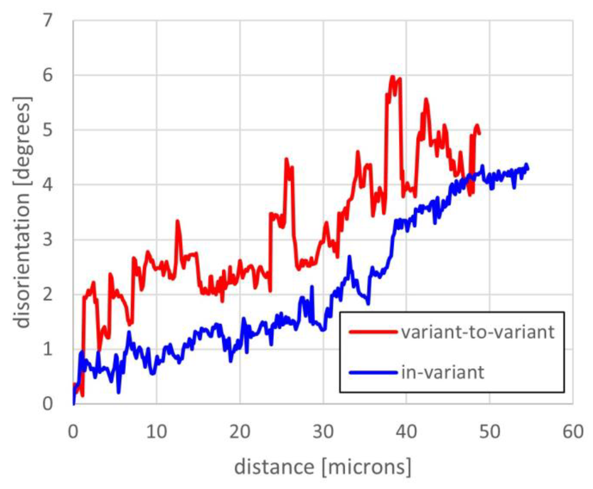
Orientation gradients were observed within individual variants and between similarly oriented variants from the same parent grain, as shown in Figure 10 for the AM Ti sample.
The implemented reconstruction algorithm assumes the orientation is constant within individual variants. The orientation associated with each variant is the average orientation over all the points within the variant [15].
After assigning each variant to a reconstructed parent grain, there are three ways to assign an orientation to each pixel within a variant. To explain these three orientation assignment methods, let ORV denote the specific symmetrical equivalent orientation relationship (OR) found between a variant and the reconstructed parent grain to which the variant belongs. The three orientation assignment methods are:
- (1)
- Each point is assigned the orientation associated with the reconstructed grain to which it belongs, denoted grain-to-point.
- (2)
- Each point is assigned the orientation calculated by applying the ORV of the variant containing the specified point to the average orientation of the variant, denoted variant-to-point.
- (3)
- Each point is assigned the orientation calculated by applying the ORV of the variant containing the point to the orientation of the specified point, denoted point-to-point.
Figure 11 shows the results for all three methods. Method 1 (Figure 11a) results in orientation gradient with large steps in orientation. Method 2 (Figure 11b) also results in an orientation gradient with large steps albeit smaller than in method 2. Method 3 results in the smoothest in-grain orientation gradient. While the true prior β microstructure is unknown, in the opinion of the authors, assignment method three, as shown in Figure 11c, is the best method for reconstructing the pre-transformation microstructure as it offers a microstructure more closely aligned with the expected in-grain orientation gradients. It should be noted, that even if the microstructure before transformation were fully recrystallized, volume changes accompanying the phase transformation can generate stresses and strains, resulting in a transformation microstructure exhibiting orientation gradients. Thus, for an extension of method 1, in method 1, the reconstruction does not necessarily result in clearly delineated grains but segments the reconstructed grains into subgrains of slightly different orientation. These subgrains could be further grouped into grains, resulting in an essentially an assignment method where the orientation variation within the grain is replaced with an average orientation constant over the entire grain.
For completeness, Figure 12 shows the in-grain disorientation profile for the reconstructed β microstructure using the point-to-point reconstruction method using the same line shown in Figure 10b. In comparing this disorientation profile with the profile shown in Figure 10a, it appears the orientation gradient is slightly stronger after the reconstruction.
The stepped nature of the orientations within the reconstructed grains is partially due to the reconstruction and can be smoothed using orientation-smoothing filters [16,17,18,19]. However, these smoothing approaches are generally adapted from image processing techniques and will not entirely reflect the true nature of the local orientation variations within the prior β grains.
3.4. Orientation Relationship Refinement
After performing a reconstruction, it is possible to refine the orientation relationship. The first step in the reconstruction is to convert the plane/direction description of the OR to a disorientation. In our implementation, the disorientation is given as a quaternion (q), but that can easily be converted to an axis-angle description for a more intuitive representation.
It should be noted that while converting an OR described as a set of parallel planes and directions is straightforward, the inverse is difficult.
To refine the OR, an adaptation of the method of Nyyssönen [20] is used:
- Collect a random set of one thousand pairs of neighboring child grains (at least the first grain in the pair is random), ensuring both child grains belong to the same parent grain.
- For each pair, calculate the disorientation between each of the two grains versus that of the parent. Add both disorientations to the global disorientation.
- Divide the summed global disorientation by the number of pairs to get the average disorientation. (Note there is more to the quaternion-based disorientation averaging scheme than described here—the actual algorithm used is an adaptation of that described in reference [15]).
The reconstruction can then be performed again and further refined in an iterative process. For the case of the Ti6Al4V, the OR shown in Equation (1) can be described as an axis-angle pair disorientation as:
Note that the crystal direction shown in Equation (4) is given in integers; thus, the description is only approximate. After refinement, the refined OR was found to be only 0.37 degrees deviated from the ideal OR. In many cases, the deviation from the idealized parallel planes and directions will be small, and the refinement process described will work well. However, in other cases, the deviation will be significant. In these cases, a methodology to get a better initial estimate of the OR may be needed [6,21].
4. Conclusions
Reconstruction of the parent microstructure of AM materials can provide a better understanding of the phase transformation process and the AM process itself. For example, reconstruction provides information on the grain size prior to transformation, which can clarify the additive manufacturing process [22,23]. The presence of orientation gradients in the as-characterized material provides some insight into the plastic flow of material during the forming process. Parent reconstruction will carry any orientation gradients existing in the as-characterized microstructure to the reconstructed microstructure. This can result in both orientation gradients in the reconstructed microstructure and segmentation of the parent grains into sub-grains of similar orientation. Additional processing may be needed to coalesce these sub-grain clusters into parent grains. It should be noted that plastic flow is a complex, dynamic process [24,25]. The orientation gradients are simply indicators of plastic flow obtained in the fixed state when the EBSD measurements are collected; determining whether the deformation happens during solidification, phase transformation, and/or HIP is unclear from the EBSD measurements. Of course, EBSD data can be collected from samples at intermediate steps in the forming process. Even with intermediate samples, the EBSD measurements alone will provide only a partial picture of the forming process. Incorporating the EBSD measurements into material models is needed to obtain a more detailed understanding of the microstructural evolution at each stage of the additive manufacturing process [26].
It should be noted that a more complex analysis of the orientation gradients would be necessary to ascertain whether the orientation gradients were present in the material prior to the phase transformation, as opposed to being formed after the transformation process.
Author Contributions
Conceptualization, S.I.W., W.C.L. and M.M.N.; methodology, S.I.W. and W.C.L.; software, S.I.W. and W.C.L.; validation, S.I.W., W.C.L. and M.M.N.; formal analysis, S.I.W.; investigation, S.I.W.; resources, M.M.N.; data curation, S.I.W.; writing—original draft preparation, S.I.W.; writing—review and editing, S.I.W., W.C.L. and M.M.N.; visualization, S.I.W.; supervision, S.I.W.; project administration, S.I.W. All authors have read and agreed to the published version of the manuscript.
Funding
No external funding was received for this work.
Data Availability Statement
The data presented in this study are available on request from the corresponding author. The data are not publicly available due to privacy.
Acknowledgments
Anthony Rollett is gratefully acknowledged for providing access to the original EBSD data from the low-carbon steel sample as well as reconstruction results using the Germain et al. algorithm as implemented in the Merengue 2 software package. Seichii Suzuki and Tatsuya Fukino of TSL Solutions KK are appreciatively acknowledged for providing parent reconstruction results using the Miyamota et al. algorithm as implemented in the ROPA software package. Charles Xu and Stephen Niezgoda of Ohio State University are gratefully acknowledged for providing parent reconstruction results using their graph-cut algorithm. Thanks to Jonathan McMenamin of Gatan/EDAX for assistance with the manuscript.
Conflicts of Interest
Stuart I. Wright, William C. Lenthe and Matthew M. Nowell are employed by the company. Gatan + EDAX, Pleasanton of USA. All authors declare that the research was conducted in the absence of any commercial or financial relationships that could be construed as a potential conflict of interest.
References
- Cayron, C. Crystallographic reconstruction methods to study phase transformations by EBSD. Microsc. Microanal. 2009, 15, 396–397. [Google Scholar] [CrossRef]
- Miyamoto, G.; Iwata, N.; Takayama, N.; Furuhara, T. Mapping the parent austenite orientation reconstructed from the orientation of martensite by EBSD and its application to ausformed martensite. Acta Mater. 2010, 58, 6393–6403. [Google Scholar] [CrossRef]
- Germain, L.; Gey, N.; Mercier, R.; Blaineau, P.; Humbert, M. An advanced approach to reconstructing parent orientation maps in the case of approximate orientation relations: Application to steels. Acta Mater. 2012, 60, 4551–4562. [Google Scholar] [CrossRef]
- Ranger, C.; Tari, V.; Farjami, S.; Merwin, M.J.; Germain, L.; Rollett, A. Austenite reconstruction elucidates prior grain size dependence of toughness in a low alloy steel. Metall. Mater. Trans. A 2018, 49, 4521–4535. [Google Scholar] [CrossRef]
- Huang, C.Y.; Ni, H.C.; Yen, H.W. New protocol for orientation reconstruction from martensite to austenite in steels. Materialia 2022, 9, 100554. [Google Scholar] [CrossRef]
- Brust, A.; Payton, E.; Hobbs, T.; Sinha, V.; Yardley, V.; Niezgoda, S. Probabilistic reconstruction of austenite microstructure from electron backscatter diffraction observations of martensite. Microsc. Microanal. 2021, 27, 1035–1055. [Google Scholar] [CrossRef] [PubMed]
- Hielscher, R.; Nyyssönen, T.; Niessen, F.; Gazder, A.A. The variant graph approach to improved parent grain reconstruction. Materialia 2022, 22, 101399. [Google Scholar] [CrossRef]
- Adams, B.L.; Wright, S.I.; Kunze, K. Orientation Imaging: The Emergence of a New Microscopy. Metall. Trans. A 1993, 24, 819–831. [Google Scholar] [CrossRef]
- Nowell, M.M.; Field, D.P.; Wright, S.I.; Dingley, D.; Scutts, P.; Suzuki, S. Orientation Imaging of Recrystallization, Grain Growth and Phase Transformations using In-Situ Heating. Microsc. Microanal. 2005, 11, 1494–1495. [Google Scholar] [CrossRef]
- Wright, S.I. Random thoughts on non-random misorientation distributions. Mater. Sci. Technol. 2006, 22, 1287–1296. [Google Scholar] [CrossRef]
- Aurenhammer, F.; Klein, R.; Lee, D.-T. Handbook of Discrete and Computational Geometry; World Scientific Publishing Company: Singapore, 2013. [Google Scholar] [CrossRef]
- Delaunay, B. Sur la sphère vide. A la mémoire de Georges Voronoï. Bulletin de l’Académie des Sciences de l’URSS. Cl. Sci. Math. Nat. 1934, 6, 793–800. [Google Scholar]
- Field, D.P. Recent advances in the application of orientation imaging. Ultramicroscopy 1997, 67, 1–9. [Google Scholar] [CrossRef]
- Hata, K.; Wakita, M.; Fujiwara, K.; Kawano, K. Development of a reconstruction method of prior austenite microstructure using EBSD data of martensite. Nippon. Steel Sumitomo Met. Tech. Rep. 2017, 114, 26–31. [Google Scholar]
- Cheng, Y.; Crassidis, J.L.; Oshman, Y. Averaging quaternions. J. Guid. Control Dyn. 2007, 30, 1193–1197. [Google Scholar] [CrossRef]
- Humphreys, F.J.; Bate, P.S.; Hurley, P.J. Orientation average of electron backscattered diffraction data. J. Microsc. 2001, 201, 50–58. [Google Scholar] [CrossRef] [PubMed]
- Godfrey, A, Edge preservation near triple junctions during orientation averaging of EBSP data. Scr. Mater. 2004, 50, 1097–1101. [CrossRef]
- Cho, J.H.; Rollet, A.D.; Oh, K.H. Determination of a mean orientation in electron backscatter diffraction measurements. Metall. Mater. Trans. A 2005, 36, 3427–3438. [Google Scholar] [CrossRef]
- Chen, D.; Kuo, J.C. Bilateral filter-based orientation smoothing of EBSD data. Ultramicroscopy 2010, 110, 1297–1305. [Google Scholar] [CrossRef]
- Nyyssönen, T. Quenching and Partitioning of High-Aluminum Steels. Ph.D. Thesis, Tamper University of Technology, Tampere, Finland, 2017. Available online: http://urn.fi/URN:ISBN:978-952-15-3896-4 (accessed on 17 December 2023).
- Nyyssönen, T.; Isakov, M.; Peura, P.; Kuokkala, V.T. Iterative determination of the orientation relationship between austenite and martensite from a large amount of grain pair misorientations. Metall. Mater. Trans. A 2016, 47, 2587–2590. [Google Scholar] [CrossRef]
- Gockel, J.; Sheridan, L.; Narra, S.P.; Klingbeil, N.W.; Beuth, J. Trends in solidification grain size and morphology for additive manufacturing of Ti-6Al-4V. JOM 2017, 69, 2706–2710. [Google Scholar] [CrossRef]
- Bermingham, M.; StJohn, D.; Easton, M.; Yuan, L.; Dargusch, M. Revealing the mechanisms of grain nucleation and formation during additive manufacturing. JOM 2020, 72, 1065–1073. [Google Scholar] [CrossRef]
- Wang, Y.; Guo, W.; Xie, Y.; Li, H.; Zeng, C.; Xu, M.; Zhang, H. In-situ monitoring plume, spattering behavior and revealing their relationship with melt flow in laser powder bed fusion of nickel-based superalloy. J. Mater. Res. Technol. 2024, 177, 44–58. [Google Scholar] [CrossRef]
- Qu, M.; Guo, Q.; Escano, L.I.; Nabaa, A.; Hojjatzadeh, S.M.H.; Young, Z.A.; Chen, L. Controlling process instability for defect lean metal additive manufacturing. Nat. Commun. 2022, 13, 1079. [Google Scholar] [CrossRef]
- Pauza, J.G.; Tayon, W.A.; Rollett, A.D. Computer simulation of microstructure development in powder-bed additive manufacturing with crystallographic texture. Model. Simul. Mater. Sci. Eng. 2021, 29, 055019. [Google Scholar] [CrossRef]
Figure 1.
(a) Color scheme used for all IPF maps in the paper for cubic (top) and hexagonal (bottom) phases, i.e., the color shows the crystal plane normally aligned in a specified sample direction. IPF maps for a low-carbon steel sheet sample. (b) As-acquired ESBD data from the transformed bcc microstructure and after reconstruction using (c) the adapted Ranger et al. algorithm [4], (d) the Germain et al. algorithm [3], (e) the Brust et al. [6] algorithm, and (f) the Miyamoto et al. [2] algorithm. The sample direction for these IPF maps is the normal direction in the rolled sheet, which is the horizontal direction in the map.

Figure 2.
IPF||ND maps for (a) the α phase and (b) the retained β phase of Ti6Al4V.

Figure 3.
IPF||ND maps for the β phase of Ti6Al4V reconstructed via (a) dilation of the grains of the retained β phase, (b) tessellation of the grains of the retained β phase, and (c) probabilistic reconstruction algorithm.
Figure 3.
IPF||ND maps for the β phase of Ti6Al4V reconstructed via (a) dilation of the grains of the retained β phase, (b) tessellation of the grains of the retained β phase, and (c) probabilistic reconstruction algorithm.

Figure 4.
Orientation map of the reconstructed β microstructure of Ti6Al4V without inclusion of the retained β grains.
Figure 4.
Orientation map of the reconstructed β microstructure of Ti6Al4V without inclusion of the retained β grains.

Figure 5.
IPF||ND maps of cobalt (colored according to the crystal direction aligned with the normal direction of the sample) at room temperature for (a) the hexagonal α phase and (b) the cubic β phase, and at high temperature for (c) the α phase and (d) the β phase.
Figure 5.
IPF||ND maps of cobalt (colored according to the crystal direction aligned with the normal direction of the sample) at room temperature for (a) the hexagonal α phase and (b) the cubic β phase, and at high temperature for (c) the α phase and (d) the β phase.

Figure 6.
(a) Indexed EBSD pattern for the low-temperature hexagonal α phase, with the (0001) pole highlighted in red. (b) SEM micrograph of the partially transformed cobalt structure. The red marker shows the location from which the EBSD pattern shown in (a) was obtained and the yellow marker showing the location for the EBSD pattern in (c). (c) Indexed EBSD pattern for the high-temperature cubic β phase, with the (111) pole highlighted in yellow.

Figure 7.
IPF||ND map of the high-temperature β microstructure of cobalt from EBSD measurements from the low-temperature α microstructure.
Figure 7.
IPF||ND map of the high-temperature β microstructure of cobalt from EBSD measurements from the low-temperature α microstructure.

Figure 8.
IPF||ND maps for (a) the original post-transformation microstructure—α phase only, (b) the reconstructed β pre-transformation microstructure, (c) the reconstructed pre-transformation microstructure after coarsening by a factor of 4, (d) 16, (e) 64, and (f) 256. See Figure 1f for the color mapping scheme.

Figure 9.
A plot of the fraction of matching points between the coarsened/reconstructed and reconstructed/coarsened datasets as a function of coarsening factor is shown. In addition, the number of measurement pixels as a function of coarsening factor is also shown.
Figure 9.
A plot of the fraction of matching points between the coarsened/reconstructed and reconstructed/coarsened datasets as a function of coarsening factor is shown. In addition, the number of measurement pixels as a function of coarsening factor is also shown.

Figure 10.
(a) Profile lines overlaid on the IPF||ND for the Ti6Al4V microstructure. (b) Disorientation profiles for variant-to-variant and in-variant within Ti6Al4V.
Figure 10.
(a) Profile lines overlaid on the IPF||ND for the Ti6Al4V microstructure. (b) Disorientation profiles for variant-to-variant and in-variant within Ti6Al4V.

Figure 11.
IPF||ND of maps of the reconstructed β microstructure using the (a) grain-to-point, (b) variant-to-point, and (c) point-to-point orientation assignment methods.
Figure 11.
IPF||ND of maps of the reconstructed β microstructure using the (a) grain-to-point, (b) variant-to-point, and (c) point-to-point orientation assignment methods.

Figure 12.
Disorientation profiles matching those shown in Figure 10a but for the reconstructed β grain.
Figure 12.
Disorientation profiles matching those shown in Figure 10a but for the reconstructed β grain.


Table 1.
Average EDS counts by phase for the lower magnification scan.
| Element | α | β | α/β |
|---|---|---|---|
| Titanium | 1459 | 1424 | 1.02 |
| Aluminum | 185 | 221 | 0.83 |
| Vanadium | 278 | 308 | 0.84 |
Disclaimer/Publisher’s Note: The statements, opinions and data contained in all publications are solely those of the individual author(s) and contributor(s) and not of MDPI and/or the editor(s). MDPI and/or the editor(s) disclaim responsibility for any injury to people or property resulting from any ideas, methods, instructions or products referred to in the content. |
© 2023 by the authors. Licensee MDPI, Basel, Switzerland. This article is an open access article distributed under the terms and conditions of the Creative Commons Attribution (CC BY) license (https://creativecommons.org/licenses/by/4.0/).
Share and Cite
MDPI and ACS Style
Wright, S.I.; Lenthe, W.C.; Nowell, M.M. Parent Grain Reconstruction in an Additive Manufactured Titanium Alloy. Metals 2024, 14, 51. https://doi.org/10.3390/met14010051
AMA Style
Wright SI, Lenthe WC, Nowell MM. Parent Grain Reconstruction in an Additive Manufactured Titanium Alloy. Metals. 2024; 14(1):51. https://doi.org/10.3390/met14010051
Chicago/Turabian StyleWright, Stuart I., William C. Lenthe, and Matthew M. Nowell. 2024. "Parent Grain Reconstruction in an Additive Manufactured Titanium Alloy" Metals 14, no. 1: 51. https://doi.org/10.3390/met14010051
Note that from the first issue of 2016, this journal uses article numbers instead of page numbers. See further details here.