The Unified Creep-Fatigue Equation for Stainless Steel 316

Abstract

Background—The creep-fatigue properties of stainless steel 316 are of interest because of the wide use of this material in demanding service environments, such as the nuclear industry. Need—A number of models exist to describe creep-fatigue behaviours, but they are limited by the need to obtain specialized coefficients from a large number of experiments, which are time-consuming and expensive. Also, they do not generalise to other situations of temperature and frequency. There is a need for improved formulations for creep-fatigue, with coefficients that determinable directly from the existing and simple creep-fatigue tests and creep rupture tests. Outcomes—A unified creep-fatigue equation is proposed, based on an extension of the Coffin-Manson equation, to introduce dependencies on temperature and frequency. The equation may be formulated for strain as ${\mathsf{\epsilon }}_p=C_{0}c\left(T,t,{\mathsf{\epsilon }}_p\right)N^{-{\mathsf{\beta }}_0}$, or as a power-law ${\mathsf{\epsilon }}_p=C_{0}c\left(T,t\right)N^{-{\mathsf{\beta }}_{0}b\left(T,t\right)}$. These were then validated against existing experimental data. The equations provide an excellent fit to data (r² = 0.97 or better). Originality—This work develops a novel formulation for creep-fatigue that accommodates temperature and frequency. The coefficients can be obtained with minimum experimental effort, being based on standard rather than specialized tests.

1. Introduction

The life of nuclear power plants has been a major issue because it strongly relates to safety and economy [1]. Stainless steel 316 is widely used for the making of components, such as turbine blades and piping, because of its excellent corrosion resistance.

As the two main fatigue evaluation and design methods in the nuclear industry, the linear damage rule and the crack growth law have been used for many years. However, microstructural characteristics lead to imperfect prediction of fatigue failure. The coefficients in these models are obtained from a large number of experiments, which are time-consuming and expensive for industry to perform. When these models are employed, the coefficients are normally obtained from specific temperature and frequency, so these coefficients cannot be used to predict fatigue life in other situations. Therefore, there is a need to develop a creep-fatigue model that can largely avoid the influence of microstructure, present the influence of creep effects on fatigue behaviour, and be generalised to other situations of temperature and frequency. Ideally, the parameters in this model should be easy to obtain from empirical tests with minimum effort.

In this paper, the strain-form unified creep-fatigue equation and power-law form will be introduced and will be verified on stainless steel 316. As part of the validation, the simple experimental methods of extracting coefficients will be presented.

2. Existing Approaches

In the case of pure fatigue, three general fatigue models are used to predict the fatigue life of this material: the Basquin equation (Equation (1)) [2], the Coffin-Manson equation (Equation (2)) [3,4] and Morrow’s energy-based equation (Equation (3)) [5,6].

$$\frac{\mathrm{∆}\mathsf{\sigma }}{2}={\mathsf{\sigma }}_f^{\prime }{\left(2N_f\right)}^b$$

(1)

$$\frac{\mathrm{∆}{\mathsf{\epsilon }}_p}{2}={\mathsf{\epsilon }}_f^{\prime }{\left(2N_f\right)}^c$$

(2)

$$\mathrm{∆}{W}_P=W_f^{\prime }{\left(2N_f\right)}^{\mathsf{\beta }}$$

(3)

where Δσ is the stress amplitude, ${\mathsf{\sigma }}_f^{\prime }$ is the fatigue strength coefficient, b is the fatigue strength exponent, Δε_p is the plastic strain amplitude, ${\mathsf{\epsilon }}_f^{\prime }$ is the fatigue ductility coefficient, c is the fatigue ductility exponent, ΔW_p is the plastic energy, $W_f^{\prime }$ is the energy coefficient, β is the energy exponent and N_f is the number of cycles. The coefficients in Equations (1) and (2) can be related through the compatibility (Equation (4)) [7] and cyclic stress-strain relation (Equation (5)) [8].

$$K^{\prime }=\frac{{\mathsf{\sigma }}_f^{\prime }}{{\left({\mathsf{\epsilon }}_f^{\prime }\right)}^{n^{\prime }}}{n}^{\prime }=\frac{b}{c}$$

(4)

$${\mathsf{\epsilon }}_p={\left(\frac{{\mathsf{\sigma }}_a}{K^{\prime }}\right)}^{\raisebox{1ex}{$1$}\!\left/ \!\raisebox{-1ex}{$n^{\prime }$}\right.}$$

(5)

where σ_a is the stress amplitude, K′ is the strain hardening coefficient and n′ is the strain hardening exponent.

In nuclear power plants, some components which are made of stainless steel 316 are subjected to fatigue at elevated temperature, at which the mechanism of creep is active. The failure of these components is caused by the combination of fatigue damage and creep damage. Two major rules are used to evaluate creep-fatigue life: the linear damage rule and the crack growth law.

2.1. The Linear Damage Rule

The linear damage theory was proposed by Palmgren [9] in 1924; it was further developed by Miner [10] in 1945 and called the Palmgren-Miner rule. This rule is widely used in the nuclear industry to design and evaluate the life of nuclear power plants [11,12,13,14]. According to this rule, damage can be calculated through using Equation (6), and the engineering structure fails when D equals 1.

$$D={\displaystyle \sum }_{i=1}^k\frac{n_i}{N_i}$$

(6)

where D is the accumulated fatigue damage, k is the number of block loading, n_i is the number of constant amplitude cycles under the ith strain/stress range, and N_i is the number of cycles to fatigue failure under the ith strain/stress range.

Combined with the creep effects, the total damage is divided into fatigue damage and creep damage at the elevated temperature (Equation (7)) [15], which shows that the accumulation of fatigue and creep damage happens at different stages.

$$D=D_f+D_c$$

(7)

where D_f is the fatigue damage and D_c is the creep damage.

However, as one of the simplified methods which are used to predict life in the nuclear industry, the linear damage rule can lead to inaccurate results because of the neglect of loading sequences [13]. This problem was also realized in other industries. Therefore, many studies were conducted to improve the accuracy of this rule. For example, Richard and Newmark [16] proposed a power-law damage rule. Manson [17] demonstrated that failure can still happen when D is less than 1 and the linear damage rule was modified to double linear damage rule. Although these models can improve the results, these modifications do not change the character of linear accumulation of damage. Therefore, when creep is active, the inaccuracy which comes from the linear accumulation of creep damage and fatigue damage still cannot be solved, because the linear addition of damage is inconsistent with the microstructural characteristics. To be specific, cyclic strain/stress causes the slips between lattices, which can lead to the persistent slip bands. These deformations then lead to cracks. Meanwhile, the damage caused by creep comes from diffusion and dislocation along the grain boundaries and within the lattice, which leads to the accumulation of voids.

2.2. The Linear Damage Rule

The crack growth law is also used in the nuclear industry to predict fatigue life of some components [18,19], such as piping and tanks. The crack growth law shows that the fatigue life is the number of loading cycles which is required to achieve the final crack size, and this process is divided into two stages: initiation and propagation. Therefore, the total crack size can be presented as the linear addition of initial crack size and propagative crack size. Normally, the initial crack is identified as the real crack size in the structures before loading, and the propagative crack (Equation (8)) [19,20] can be obtained through Paris’s model [21]:

$$\frac{\mathrm{d}a}{\mathrm{d}N}=C{\left(\mathrm{∆}{J}_{\mathrm{eff}}\right)}^l$$

(8)

where $\frac{\mathrm{d}a}{\mathrm{d}N}$ is the total crack growth per cycle, ΔJ_eff is the effective range of J-integral, and C is a material constant obtained from experiments. When creep is active, the total damage is calculated through the sum of fatigue and creep crack growth (Equations (9a) and (9b)) [21]:

$$\frac{\mathrm{d}a}{\mathrm{d}N}={\left(\frac{\mathrm{d}a}{\mathrm{d}N}\right)}_f+{\left(\frac{\mathrm{d}a}{\mathrm{d}N}\right)}_c$$

(9a)

$${\left(\frac{\mathrm{d}a}{\mathrm{d}N}\right)}_f=C{\left(\mathrm{∆}{J}_{\mathrm{eff}}\right)}^l\text{ and }{\left(\frac{\mathrm{d}a}{\mathrm{d}N}\right)}_c={\int }_0^{t_h}A{C}^{*q}\mathrm{d}t$$

(9b)

where ${\left(\frac{\mathrm{d}a}{\mathrm{d}N}\right)}_f$ is the crack growth per cycle due to cyclic load changes, ${\left(\frac{\mathrm{d}a}{\mathrm{d}N}\right)}_c$ is the crack growth per cycle due to hold time, t_h is the hold time, $C^{*}$ is the time-dependent fracture parameter, and l, A and q are material constants obtained from experiments.

The crack growth law provides a good physical explanation of damage. However, the quantitative summation between the cracks caused by fatigue and the cracks caused by creep does not consider the directions of these cracks. This means that two parallel cracks can cause the same damage as two non-parallel cracks, which is inconsistent with the microstructure, because the angle between two cracks plays an important role in the total damage.

2.3. Recent Developments towards a Unified Creep-Fatigue Equation

As identified above, the limitations of these methods are that they do not fully accommodate the observed microstructural characteristics, they require extensive testing to determine the coefficients, and the results cannot be generalised to other situations of temperature and frequency.

In an attempt to address these problems, Wong and Mai [22] proposed a formalism to accommodate fatigue and creep-fatigue, which they called a unified creep-fatigue equation (hereafter WM equation); see Equation (10). The unified creep-fatigue equation takes into account the influence of temperature and frequency on fatigue life. This equation was developed by extension of the Coffin-Manson equation.

$${\mathsf{\epsilon }}_p=C_{0}s\left(\mathsf{\sigma }\right)c\left(T,t\right)N^{-{\mathsf{\beta }}_{0}b\left(T,t\right)}$$

(10)

where σ is the stress, T is the temperature, t is the cyclic time (1/frequency), C₀ is the fatigue ductility coefficient, β₀ is the fatigue ductility exponent, ε_p is the plastic strain and N is the fatigue life. The basic premise of the WM formulation is that ‘all fatigue phenomenon are indeed creep-fatigue, and “pure fatigue” is just a special case of creep-fatigue’ [22]. They reasoned that the Coffin-Manson equation was “a special case of a unified creep-fatigue equation”.

The general principles of this were shown for the case of SnPb solder [22]. However there are several issues with the WM formulation. They did not provide the method to get the stress function s (σ). This means that this unified equation still cannot be used to predict fatigue life. A related issues is that they assumed that functions c (T, t) and b (T, t) share the same pattern and characteristics, such that internal coefficients c₁/c₂ = b₁/b₂, but no reason was provided for this assumption. Also, the method of extracting the coefficients of function c (T, t) and b (T, t) was not proposed.

The WM equation has potential, but the concept needs further development. It has not been applied other than to solder, so its universal applicability is uncertain. There is a need to further validate or modify and the relationships between the coefficients, or improve the formulation.

3. Methods

3.1. Research Question

The purpose of this paper was to extend and modify the WM unified creep-fatigue equation. The WM equation provided some helpful initial starting points for the present work. Firstly, they showed that the creep-fatigue behaviour is negatively influenced by temperature, frequency and stress. Secondly, the unified creep-fatigue equation could be deduced from the Coffin-Manson equation and the experimental data of Shi [23] on solder, and the reference condition could be introduced into this unified equation. Thirdly, function c (T, t) and b (T, t) could be related to Manson-Haferd parameter, at least numerically.

3.2. Approach

Work in progress towards a further conceptual development has been to show how plastic strain (ε_p) may be theoretically related, in the creep-fatigue situation, to conditions at the reference temperature (T_ref) and reference cycle time (t_ref) at which tests are performed [24]. This line of thinking results in two forms of the unified creep-fatigue equation. The first form (strain form) represents the plastic strain as a function of cycle time, number of cycles, and temperature: ${\mathsf{\epsilon }}_p=C_{0}c\left(T,t,{\mathsf{\epsilon }}_p\right)N^{-{\mathsf{\beta }}_0}$. The second form (power-law form) does the same, but is simplified to a power-law relationship: ${\epsilon }_p=C_{0}c\left(T,t\right)N^{-{\mathsf{\beta }}_{0}b\left(T,t\right)}$. Definitions of variables are provided below.

In this paper both forms are verified by application to stainless steel 316. As part of the validation, the simple experimental methods of extracting coefficients are presented. The approach is to take published empirical data for creep rupture tests and creep-fatigue tests. The experimental data for creep-fatigue are from [25] and the creep rupture data are from [26] for stainless steel 316. From the data which were obtained at an arbitrary temperature and reference cycle time, we extract coefficients for the strain-form unified creep-fatigue equation (Section 4.3.1), and validate them through the empirical data at other conditions (Section 4.3.2). Then, the empirical data at two temperatures and reference cycle time are used to extract the coefficients for the power-law form (Section 4.4.1.1 and Section 4.4.2.1), and validate it through the empirical data at other conditions (Section 4.4.1.2 and Section 4.4.2.2).

The unified creep-fatigue equations were originally developed for solder, a material that is very different to stainless steel. Results show that the two forms of the unified creep-fatigue equation provide excellent representation of the stainless steel 316 creep fatigue data. A temperature modified Coffin-Manson equation was derived from the combination of the power-law unified creep-fatigue equation and the frequency modified Coffin-Manson equation.

4. Results: Theory and Calculation

4.1. Introduction to the Unified Creep-Fatigue Equation

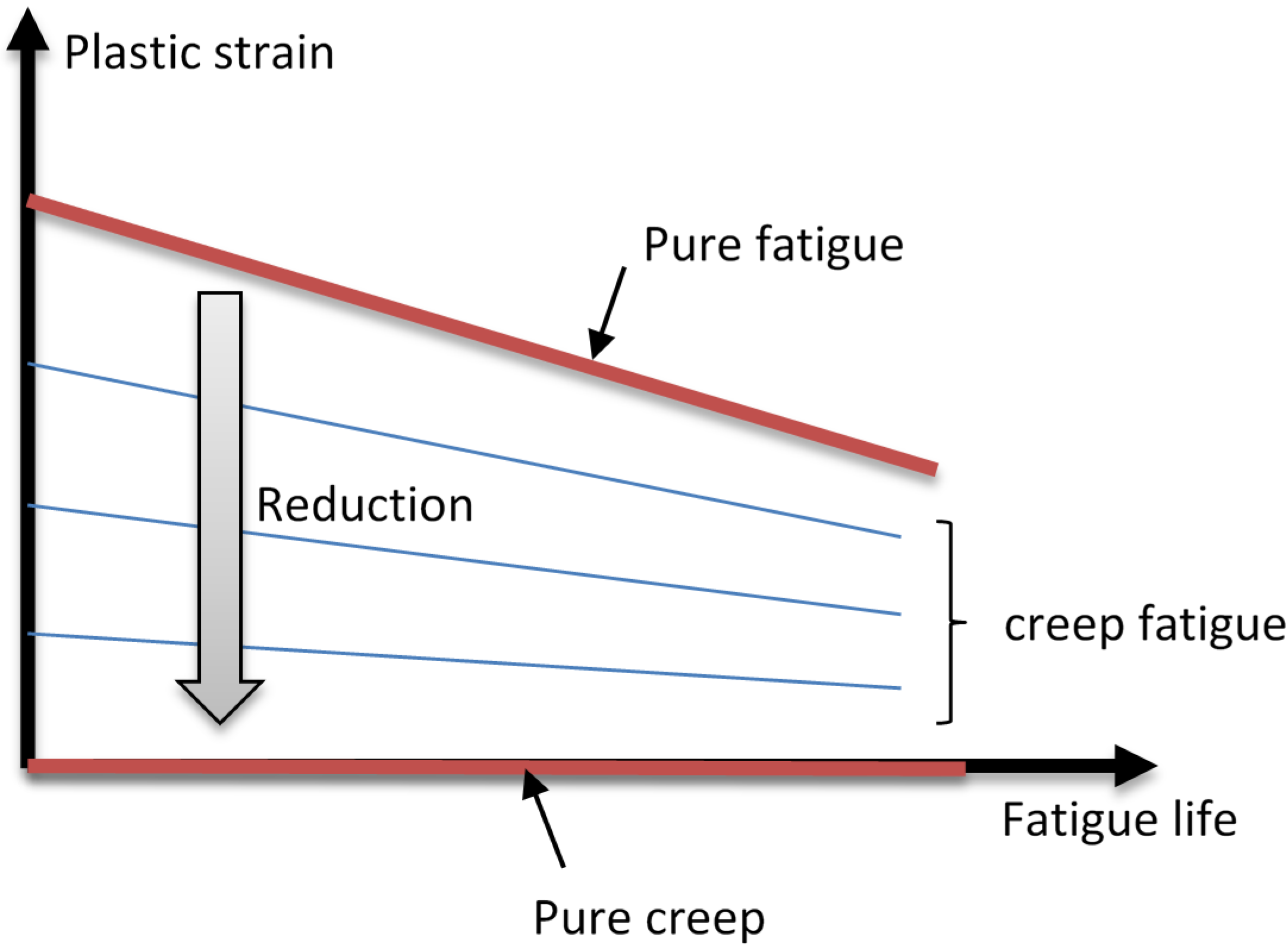
At this point, the term “fatigue capacity” needs to be introduced to describe the relation between pure fatigue and creep. For creep-fatigue, the fatigue capacity is reduced because of the increasing influence of creep damage. This can be seen in Figure 1: the creep-fatigue curves between pure fatigue curve and pure creep curve show the residual fatigue capacities, and the reductions are caused by creeps at different plastic strains/stresses.

Therefore, given the contribution of creep to the reduction of fatigue capacity, it is reasonable that the time-temperature-stress relationship, such as the Sherby-Dorn Parameter (Equation (11)) [27], the Larson-Miller Parameter (Equation (12)) [28] and the Manson-Haferd Parameter (Equation (13)) [29], is involved in the unified creep-fatigue equation.

$$P_{\mathrm{SD}}\left(\mathsf{\sigma }\right)=t{e}^{-Q/RT}$$

(11)

$$P_{\mathrm{LM}}\left(\mathsf{\sigma }\right)=T\left(\log t+C\right)$$

(12)

$$P_{\mathrm{MH}}\left(\mathsf{\sigma }\right)=\frac{T-T_a}{\log t-\log t_a}$$

(13)

where P_SD is the Sherby-Dorn Parameter, P_LM is the Larson-Miller Parameter, P_MH is the Manson-Haferd Parameter, Q is the activation energy of the creep mechanism, R is the Boltzmann’s constant, t is the time, T is the absolute temperature, C is a constant and ($\log t_a$, $T_a$) is the point of convergence of the $\log t–T$ lines. Among these three parameters, the Manson-Haferd Parameter is regarded as the best description of stress-time-temperature relation [30].

It can be found that the unified creep-fatigue equation (Equations (14) and (15)) [24] shows a linear relationship between T and logt:

$${\mathsf{\epsilon }}_p=C_{0}c\left(T,t,{\mathsf{\epsilon }}_p\right)N^{-{\mathsf{\beta }}_0}$$

(14)

with

$$c\left(T,t,{\mathsf{\epsilon }}_p\right)=1-c_1\left({\mathsf{\epsilon }}_p\right)\left(T-T_{\mathrm{ref}}\right)-c_2\log \left(t/t_{\mathrm{ref}}\right)(T>T_{\mathrm{ref}},t>t_{\mathrm{ref}})$$

(15)

Note that this relationship is consistent with the form of the P_MH parameter.

The reference condition refers to the threshold temperature T_ref at which creep first occurs (below this temperature no creep occurs), and cycle time (period) t_ref (arbitrary set as 1 second for comparing different data sets). The reference temperature and cyclic time for stainless steel 316 are identified as T_ref = 670 K and t_ref = 1 s. This temperature is 0.4 of the melting temperature and corresponds to the widely held assumption that below this temperature no creep occurs.

We then determine the plastic strain at reference condition, by transforming Equation (14):

$${\mathsf{\epsilon }}_{p,\mathrm{ref}}=C_0{N}^{-{\mathsf{\beta }}_0}=\frac{{\mathsf{\epsilon }}_p}{c\left(T,t,{\mathsf{\epsilon }}_p\right)}$$

(16)

This transformation would result in all ε_p: N data reducing into one single ε_p,ref: N curve if the creep function (Equation (15)) could describe the influence of creep on fatigue well.

However, the strain form returns an equation that is not power-law. Because power-law relation is expressed as a straight line on a log-log plot, it can provide an easy and clear way to present the creep-fatigue behaviours between different temperatures and cyclic times through translation and rotation. For this reason, the unified creep-fatigue equation is represented as a power-law form (Equation (17)) [24] through fitting the ε_p-N data with a power-law relation.

$${\mathsf{\epsilon }}_p=C_{0}c\left(T,t\right)N^{-{\mathsf{\beta }}_{0}b\left(T,t\right)}$$

(17)

with

$$c\left(T,t\right)=1-c_1\left(T-T_{ref}\right)-c_2\log \left(t/t_{ref}\right)(T>T_{\mathrm{ref}},t>t_{\mathrm{ref}})$$

(18)

$$b\left(T,t\right)=1-b_1\left(T-T_{\mathrm{ref}}\right)-b_2\log \left(t/t_{\mathrm{ref}}\right)(T>T_{\mathrm{ref}},t>t_{\mathrm{ref}})$$

(19)

Then, the plastic strain at reference condition is determined by transforming Equation (17):

$${\mathsf{\epsilon }}_{p,\mathrm{ref}}=C_0{N}^{-{\mathsf{\beta }}_0}=C_0{\left[\frac{{\mathsf{\epsilon }}_p}{C_{0}c\left(T,t\right)}\right]}^{1/b\left(T,t\right)}$$

(20)

This transformation would cause all ε_p:N data to collapse into one ε_p,ref:N curve if the creep function (Equation (18)) and stress function (Equation (19)) could present the influence of creep on fatigue well.

It can be seen that the unified creep-fatigue equation is restored to the Coffin-Manson equation at reference condition (T_ref, t_ref), which builds a bridge between pure fatigue and creep fatigue. The deduction of coefficients (Equations (A1)–(A13)) in the strain-form unified creep-fatigue equation and power-law form is shown in Appendix A.

Next, the relatively simple methods of obtaining the coefficients will be verified on stainless steel 316.

4.2. Extracting the Creep-Rupture Properties of Stainless Steel 316

The Manson–Haferd parameter was extracted through plotting creep-rupture data [26] as log (time) vs. temperature. According to the Manson-Haferd parameter, all logt–T lines at different stresses should converge to one point, where the temperature is regarded as the Creep Initiation Temperature, below which no creep occurs. We determine this temperature as 40% of the melting temperature. This corresponds to the reference temperature. In this case the reference temperature is found to be T_ref = 670 K. At this temperature, the rupture times at different stresses were found. According to Manson-Haferd parameter, these rupture times should be the same. However, because the accuracy of experiments is influenced by many factors, such as facilities and environment, the points (rupture time, reference temperature) at different stresses cannot be collected into one point. Therefore, the average of these rupture times is employed to define the rupture time at the point of convergence, and the point of convergence is identified to be (670, 9.54) (shown in Figure 2). The Manson-Haferd parameter is stress dependent, and the values are obtained as the inverse of the slope from the fitted lines. Then, the relationship between Manson-Haferd parameter and stress can be extracted from Figure 2, and Equation (21) is given through curve-fitting:

$$-\frac{1}{P_{\mathrm{MH}}\left(\mathsf{\sigma }\right)}=4.50\times {10}^{-3}+1.26\times {10}^{-5}\mathsf{\sigma }+1.70\times {10}^{-7}{\mathsf{\sigma }}^2$$

(21)

To convert P_MH (σ) to P_MH (ε_p), the data of stress, total strain, temperature and Young’s modulus are extracted from [31]. Because the time of tension tests is much less than the creep-rupture time, the influence of time (creep) on tension tests can be neglected. The temperature-dependent plastic strain-stress relationship (Equations (22)–(24)) can be developed through curve-fitting.

$${\mathsf{\epsilon }}_p={\left(\frac{\mathsf{\sigma }}{K\left(T\right)}\right)}^{1/n\left(T\right)}$$

(22)

$$K\left(T\right)=-0.4875T+769.79$$

(23)

$$n\left(T\right)=7.04\times {10}^{-2}+1.94\times {10}^{-4}T-1.22\times {10}^{-7}{T}^2$$

(24)

Then, substituting Equations (22)–(24) into Equation (21) gives Equation (25):

$$-\frac{1}{P_{\mathrm{MH}}\left({\mathsf{\epsilon }}_p,T\right)}=4.50\times {10}^{-3}+1.26\times {10}^{-5}K\left(T\right){\mathsf{\epsilon }}_p^{n\left(T\right)}+1.70\times {10}^{-7}K\left(T\right){\mathsf{\epsilon }}_p^{2n\left(T\right)}$$

(25)

4.3. Evaluation of the Coefficients of the Strain-Form Unified Creep-Fatigue Equation ${\epsilon }_p=C_{0}c\left(T,t,{\epsilon }_p\right)N^{-{\beta }_0}$ for the Stainless Steel 316 and Validation

4.3.1. Evaluation of Creep-Fatigue Coefficients

Based on the Equations (A1)–(A6) shown in Appendix A, the coefficients of the creep function, c (T, t, ε_p), for the stainless steel 316 are established as follows.

Substituting log t_a = 9.54 and t_ref = 1 s into Equation (A2), the coefficient c₂ is evaluated as:

$$c_2=\frac{1}{\log \left(t_a/t_{\mathrm{ref}}\right)}=\frac{1}{\log \left({10}^{9.54}/1\right)}=0.105$$

(26)

Substituting Equation (26) into Equation (A4), coefficient c₁ (σ) and c₁ (ε_p) are developed respectively:

$$c_1\left(\mathsf{\sigma },T\right)=4.73\times {10}^{-4}+1.32\times {10}^{-6}\mathsf{\sigma }\left(T\right)+1.79\times {10}^{-8}{\mathsf{\sigma }}^2\left(T\right)$$

(27)

$$c_1\left({\mathsf{\epsilon }}_p,T\right)=4.73\times {10}^{-4}+1.32\times {10}^{-6}K\left(T\right){\mathsf{\epsilon }}_p^{n\left(T\right)}+1.79\times {10}^{-8}{K}^2\left(T\right){\mathsf{\epsilon }}_p^{2n\left(T\right)}$$

(28)

The fatigue coefficients C₀ and β₀ of the stainless steel 316 can be extracted from fatigue test at an arbitrary temperature at the reference cycle time. Selecting the data point (T = 873 K, t_ref), at which ε_p (T = 873 K, t_ref, N = 1) = 2.1705, C_o is extracted through using Equation (A6), which is 2.95, and β₀ is given as 0.663. However, a big error ($\sum {\left(N_{f-\exp }-N_{f-\mathrm{equ}}\right)}^2=49.85$) is given through comparing the fatigue life obtained from experiments with the fatigue life obtained from unified creep-fatigue. Therefore, the C₀ is resolved as 0.959 through minimizing the error (0.312).

4.3.2. Validations

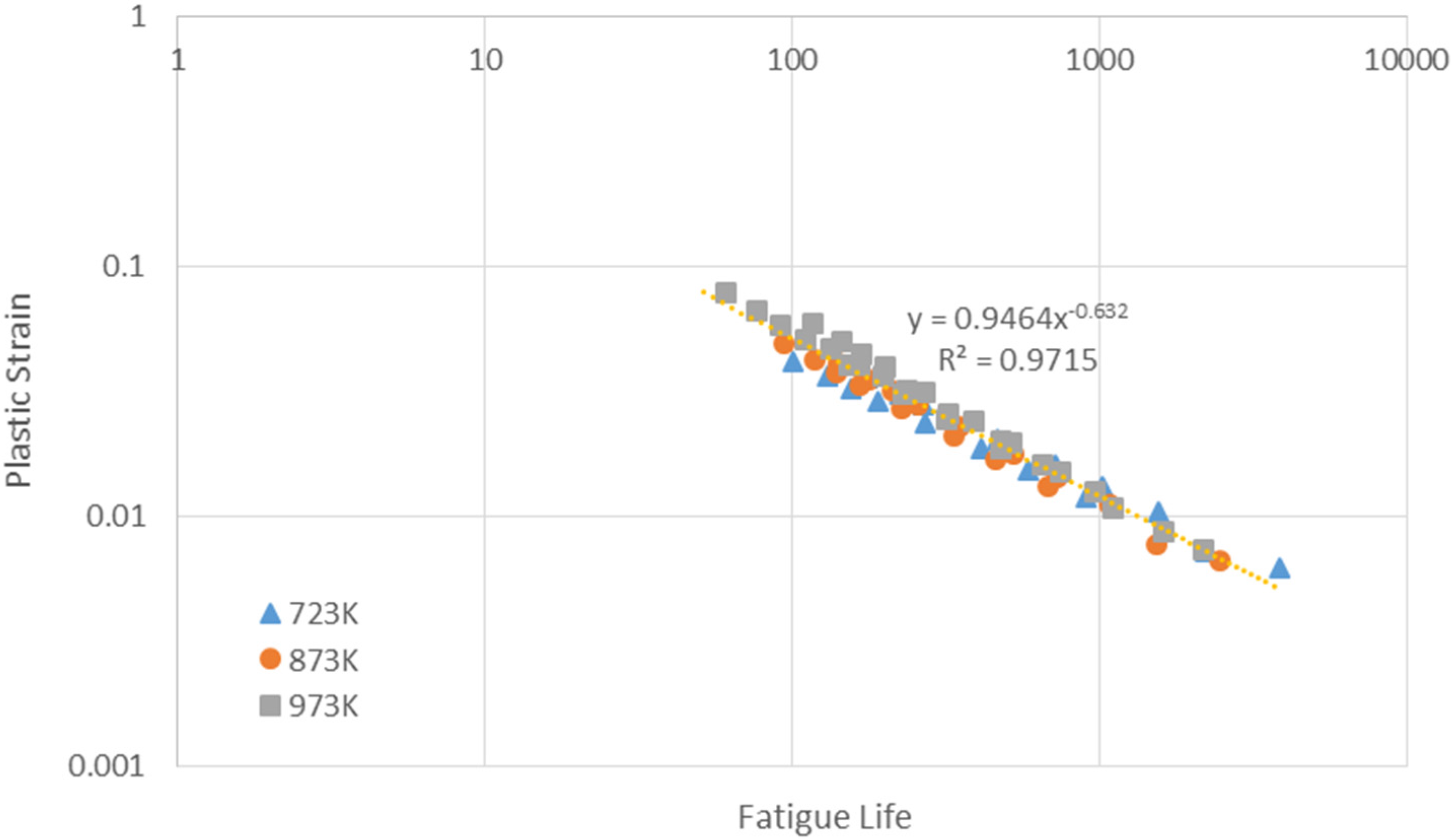
Using the fatigue and the creep coefficients evaluated in Section 4.3.1, namely, C₀ = 0.959, β₀ = 0.663, c₂ = 0.105, and c₁ (ε_p, T) as described by Equation (28), the generated raw fatigue data (ε_p–N) obtained from [25] (T = 723 K, 873 K and 973 K) are transformed to the reference condition (ε_p,ref–N) through Equation (16). The transformed data are plotted in Figure 3.

Significantly, these data are collected into a power-law curve of ${\mathsf{\epsilon }}_{p,\mathrm{ref}}=0.9464N^{-0.632}$ with the quality of fit as R² = 0.9715. This good transformation verifies the unified equation, ${\mathsf{\epsilon }}_p=C_{0}c\left(T,t,{\mathsf{\epsilon }}_p\right)N^{-{\mathsf{\beta }}_0}$, the form of creep function c (T, t, ε_p), and the methods of extracting the fatigue and the creep coefficients. The error between fatigue life from experiments and creep-fatigue equation is 0.312.

4.3.3. Application

This shows that the mathematical representation provided by the strain-form unified creep-fatigue equation accommodates the data for multiple temperatures, fatigue life, and plastic strain.

$${\mathsf{\epsilon }}_p=0.959\left[1-c_1\left({\mathsf{\epsilon }}_p,T\right)\left(T-670\right)-0.105\log \left(t\right)\right]N^{-0.663}$$

(29)

with

$$\begin{array}{ll}{c}_1\left({\mathsf{\epsilon }}_p,T\right)=4.73& \times {10}^{-4}+8.712\times {10}^{-7}\\ & \times \left(769.79-0.4875T\right){\mathsf{\epsilon }}_p^{7.04\times {10}^{-2}+1.94\times {10}^{-4}T-1.22\times {10}^{-7}{T}^2}+7.797\\ & \times {10}^{-9}\times {\left(769.79-0.4875T\right)}^2{\mathsf{\epsilon }}_p^{0.1408+3.88\times {10}^{-4}T-2.44\times {10}^{-7}{T}^2}\end{array}$$

(30)

This could be used to determine fatigue life for given plastic strain, temperature and cycle time. Alternatively, to determine plastic strain by numerical solution of the equation.

4.4. Evaluation of the Coefficients of the Power-Law Unified Creep-Fatigue Equation ${\epsilon }_p=C_{0}c\left(T,t\right)N^{-{\beta }_{0}b\left(T,t\right)}$ for the Stainless Steel 316 and Validation

The fatigue behaviour of stainless steel 316 presents an inflection point at the temperature of 873 K [25]. Below this temperature, the fatigue life decreases with the increasing temperature, while, increases above this temperature. Given that the power-law unified creep-fatigue equation is built on the assumption of continual increasing/decreasing fatigue life with increasing temperature, the evaluation and validation of the power-law unified creep-fatigue equation are conducted at two temperature regimes (below 873 K and above 873 K).

4.4.1. Evaluation of Creep-Fatigue Coefficients and Validation below 873 K

4.4.1.1. Evaluation of Creep-Fatigue Coefficients

Based on the Equations (A7)–(A13) shown in Appendix A, the coefficients of c function and b function for the stainless steel 316 are established as follows.

The creep coefficient c₂ is identical as 0.105.

Substituting Equation (18) with the data points (T = 873 K, t = t_ref) and (T = 873 K, t = 10 s), where ε_p (T = 873 K, t = t_ref, N = 1) = 1.0296 (Equation (A8)) and ε_p (T = 873 K, t = 10 s, N = 1) = 0.5987 (Equation (A9)), gives C₀c₂ = 0.4309. Then, C₀ is solved as 4.1038. In addition, substituting Equation (19) with these two data points, where β₀b (873 K, t = t_ref) = 0.663 (Equation (A10)) and β₀b (T = 873 K, t = 10 s) = 0.651 (Equation (A11)), gives β₀b₂ = 0.012.

Substituting Equation (18) with the data points (T = 723 K, t = t_ref) and (T = 873 K, t = t_ref), where ε_p (T = 723 K, t = t_ref, N = 1) = 2.1705 (Equation (A12)) and ε_p (T = 873 K, t = t_ref, N = 1) = 1.0296 (Equation (A8)), gives c₁ = 0.001853. Then, substituting Equation (19) with these two data points, where β₀b (723 K, t = t_ref) = 0.634 (Equation (A13)) and β₀b (873 K, t = t_ref) = 0.663 (Equation (A10)), gives β₀ = 0.624 and b₁ = −0.00031, then b₂ is solved as 0.01924.

The error between the fatigue life from experiments and creep-fatigue equation is 52.88. As shown in the evaluation of coefficients for strain-form unified creep-fatigue equation, this poor prediction is caused by the inaccuracy of C₀. Therefore, the C₀ is resolved as 0.876 through minimizing the error (0.792).

4.4.1.2. Validations

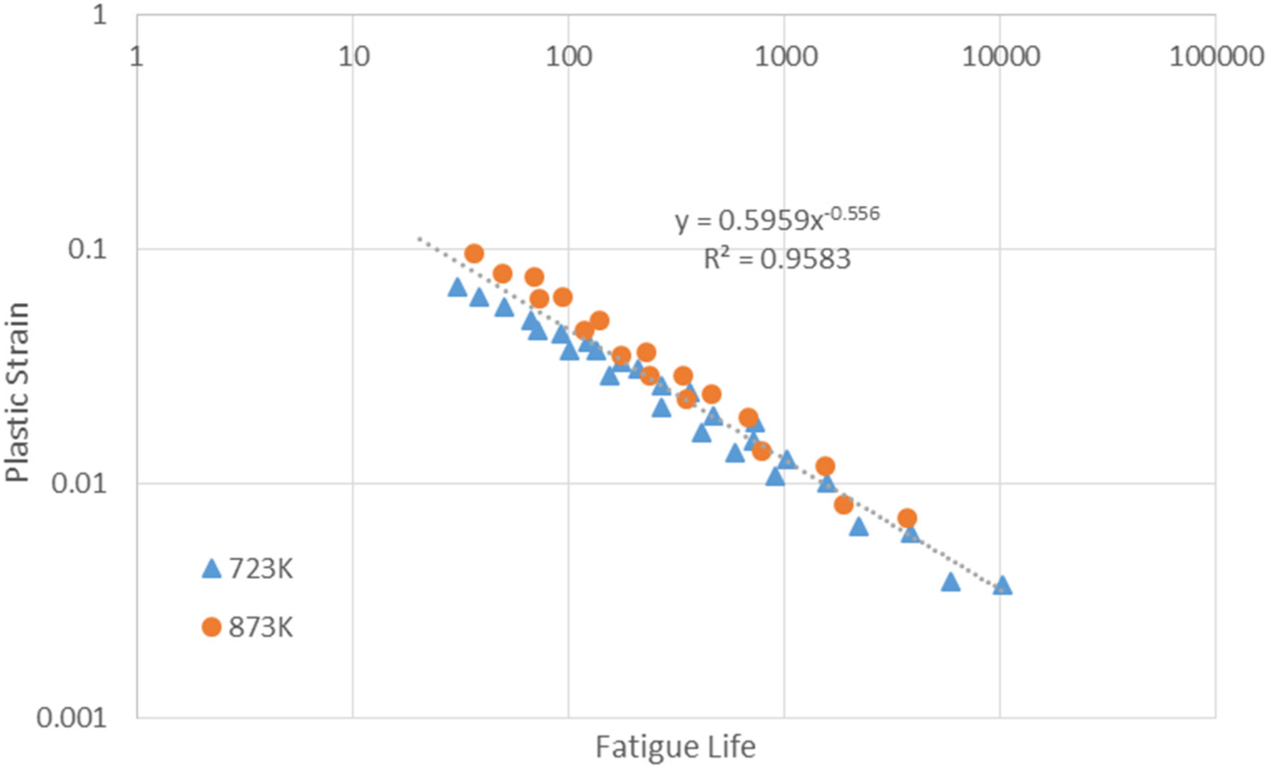
Using the fatigue and creep coefficients found in Section 4.4.1.1, namely, C₀ = 0.876, β₀ = 0.624, c₁ = 0.001853, c₂ = 0.105, b₁ = −0.0003094 and b₂ = 0.01924, the raw fatigue data (ε_p–N) obtained from [25] (T = 723 K and 873 K) are transformed to the reference condition (ε_p,ref–N) through Equation (20). The transformed data are plotted in Figure 4, which shows that these data can be collapsed into a power-law curve of ${\mathsf{\epsilon }}_{p,\mathrm{ref}}=0.5959N^{-0.556}$ with the quality of fit as R² = 0.9583. This transformation has verified the unified equation, ${\mathsf{\epsilon }}_p=C_{0}c\left(T,t\right)N^{-{\mathsf{\beta }}_{0}b\left(T,t\right)}$, the form of creep function c (T, t) and stress function b (T, t), and the methods of extracting the coefficients. The error between fatigue life from experiments and creep-fatigue equation is 0.792.

4.4.2. Evaluation of Creep-Fatigue Coefficients and Validation above 873 K

4.4.2.1. Evaluation of Creep-Fatigue Coefficients

The data points (T = 873 K, t = t_ref), (T = 873 K, t = 10 s) and (T = 973 K, t = t_ref) are selected to evaluate the coefficients. These coefficients are obtained through the same method shown in Section 4.4.1.1: C₀ = 0.879, β₀ = 0.807, c₁ = 0.00146, c₂ = 0.105, b₁ = 0.00088 and b₂ = 0.01487.

4.4.2.2. Validations

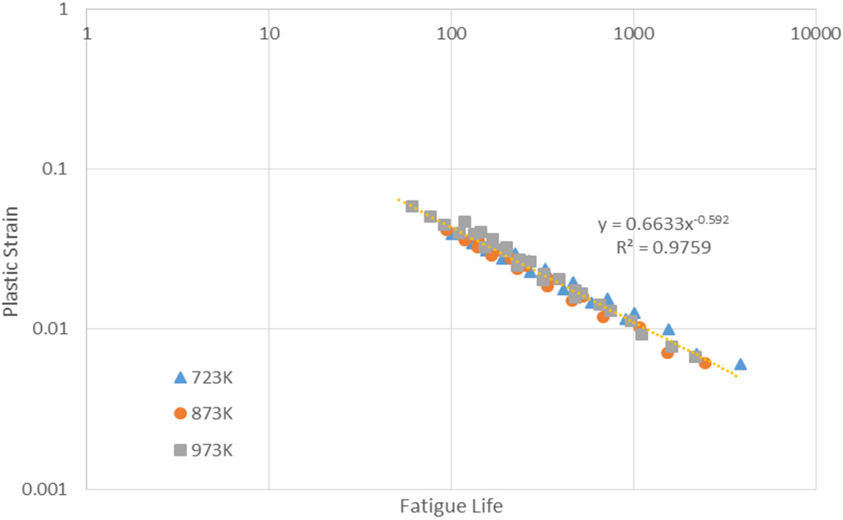
Using the fatigue and creep coefficients found in Section 4.4.2.1, the raw fatigue data (ε_p–N) obtained from [25] (T = 873 K and 973 K) are transformed to the reference condition (ε_p,ref–N) through Equation (20). The transformed data plotted in Figure 5, which shows that these data can be collapsed into a power-law curve of ${\mathsf{\epsilon }}_{p,\mathrm{ref}}=0.9439N^{-0.82}$ with a quality of fit of R² = 0.9797. This transformation has verified the unified equation, ${\mathsf{\epsilon }}_p=C_{0}c\left(T,t\right)N^{-{\mathsf{\beta }}_{0}b\left(T,t\right)}$, the form of creep function c (T, t) and stress function b (T, t), and the methods of extracting the coefficients. The error between fatigue life from experiments and creep-fatigue equation is 0.300.

4.4.3. Application

The mathematical representation (Equation (31) for below 873 K and Equation (32) for above 873 K) provided by the unified creep-fatigue equation accommodates the data for multiple temperatures, fatigue life, and plastic strain. This could be used to determine fatigue life for given plastic strain, temperature and cycle time. Alternatively, to determine plastic strain by numerical solution of the equation:

$$\begin{array}{c}{\mathsf{\epsilon }}_p=0.876[2.2415-0.001853\mathrm{T}-0.105\log \left(t\right)]N^{-0.624[0.7927+0.0003094T-0.01924\log \left(t\right)]}\\ (T<873\mathrm{K})\end{array}$$

(31)

$$\begin{array}{c}{\mathsf{\epsilon }}_p=0.879[1.9782-0.00146\mathrm{T}-0.105\log \left(t\right)]N^{-0.807[1.5896+0.00088T-0.01487\log \left(t\right)]}\\ (T\ge 873\mathrm{K})\end{array}$$

(32)

5. Discussion

5.1. The Moderating Factor

As shown above, C₀ in the strain-form unified creep-fatigue equation was obtained from data point (T = 723 K, t_ref). However, this result is different from C₀ obtained from data point (T = 873 K, t_ref) and (T = 973 K, t_ref). To improve the accuracy of C₀, these three data points are used to regress the magnitude of C₀, which is 2.517 (Equation (33)).

$${\mathsf{\epsilon }}_p\left(T,t_{\mathrm{ref}},N=1\right)=C_0^{\prime }=C_0\left[1-c_1\left(C_0^{\prime }\right)\left(T-T_{\mathrm{ref}}\right)\right]=2.517\left[1-0.00278\left(T-T_{\mathrm{ref}}\right)\right]$$

(33)

At data point (T = 723 K, t_ref), substituting $C_0^{\prime }$ into the Equation (28) cannot yield to 2.1705, and the magnitude of $c_1\left(2.1705\right)$ is bigger than 0.00278. Thus, according to the Equation (27), it appears that the big contribution of stress leads to higher magnitude of c₁ function. Therefore, mathematically, the amplitude of stress should be compressed in order to reduce the magnitude of $c_1\left(C_0^{\prime }\right)$ into the result of regression (0.00278). Then, a moderating factor, f, is introduced into Equation 27 to modify stress, and Equations (27) and (28) can be expressed as:

$$c_1\left(\mathsf{\sigma },f\right)=4.73\times {10}^{-4}+1.32\times {10}^{-6}f\mathsf{\sigma }+1.79\times {10}^{-8}{f}^2{\mathsf{\sigma }}^2$$

(34)

$$c_1\left({\mathsf{\epsilon }}_p,T,f\right)=4.73\times {10}^{-4}+1.32\times {10}^{-6}fK\left(T\right){\mathsf{\epsilon }}_p^{n\left(T\right)}+1.79\times {10}^{-8}{f}^{2}K\left(T\right){\mathsf{\epsilon }}_p^{2n\left(T\right)}$$

(35)

This moderating factor is solved as 0.69, and C₀ is given as 0.846 through minimizing the error (0.276).

Using the fatigue and the creep coefficients, namely, C₀ = 0.846, β₀ = 0.663, c₂ = 0.105, c₁ (ε_p,T, f) as described by Equation (35) and f = 0.69, the generated raw fatigue data (ε_p–N) obtained from [25] (T = 723 K, 873 K and 973 K) are transformed to the reference condition (ε_p,ref–N) through Equation (16). The transformed data are plotted in Figure 6.

Figure 6 illustrates how the transformed data are collected into a power-law curve of ${\mathsf{\epsilon }}_{p,\mathrm{ref}}=0.6633N^{-0.592}$ with the quality of fit R² = 0.9759. The error between fatigue life from experiments and creep-fatigue equation is 0.276. Comparing this result with the transformation in Section 4.3.2 shows that the introduction of moderating factor can provide a better description of creep effect through c₁ function and prediction of creep-fatigue behaviour.

The research conducted by Gary shows that the stress vs. creep rupture time curves under cyclic loading lie above the curves under constant loading [32]. This means that cyclic stress is higher than constant stress at the same rupture time. Because c₁ function is based on the time-temperature relation under constant stress (Manson-Haferd parameter), the creep effect is enlarged when the cyclic stress is imposed. Therefore, it is reasonable to introduce a moderating factor to compress the cyclic stress to an equivalent constant stress.

5.2. The Heat Treatment

Heat treatment can change fatigue behaviour through hardening or softening. However, stainless steel 316 cannot be hardened by heat treatment, and this is proved by [33], where fatigue life changes slightly between aged condition and annealed condition [33]. This makes the unified creep-fatigue equation more universal for stainless steel 316 under different heat treatments. For example, the creep-fatigue data of aged stainless steel obtained from [33] (T = 839 K and 922 K) and quenched stainless steel 316 obtained from [25] (T = 723 K, 873 K and 973 K) can be collected into one power-law curve ${\mathsf{\epsilon }}_{p,\mathrm{ref}}=0.6533N^{-0.588}$ with a quality of fit of R² = 0.9827 (Figure 7).

Although the unified creep-fatigue equation shows a good universality for stainless steel 316 under different heat treatments, the potential limitation for this equation still cannot be ignored. For example, this strong influence of heat treatment on fatigue life is shown on Inconel 718, and the aged condition can provide better fatigue strength than annealed condition [33]. Therefore, if the unified creep-fatigue equation is imposed on Inconel 718, the coefficients obtained at one specified heat treatment condition cannot be used to predict the fatigue life of this material under other heat treatments. This is an opportunity for future development of the formulation.

5.3. Reliability

The proposed new equations were validated against existing experimental data in the literature. The equations provide an excellent fit to data (r² = 0.97 or better). This demonstrates that the equations provide the desired level of fidelity to the original experimental data.

The validation only can show these selected data follow the unified creep-fatigue equation, but not all data. Hence it is important to consider the degree of reliability. In this section, the strain-form unified creep-fatigue equation was used to explore the reliability.

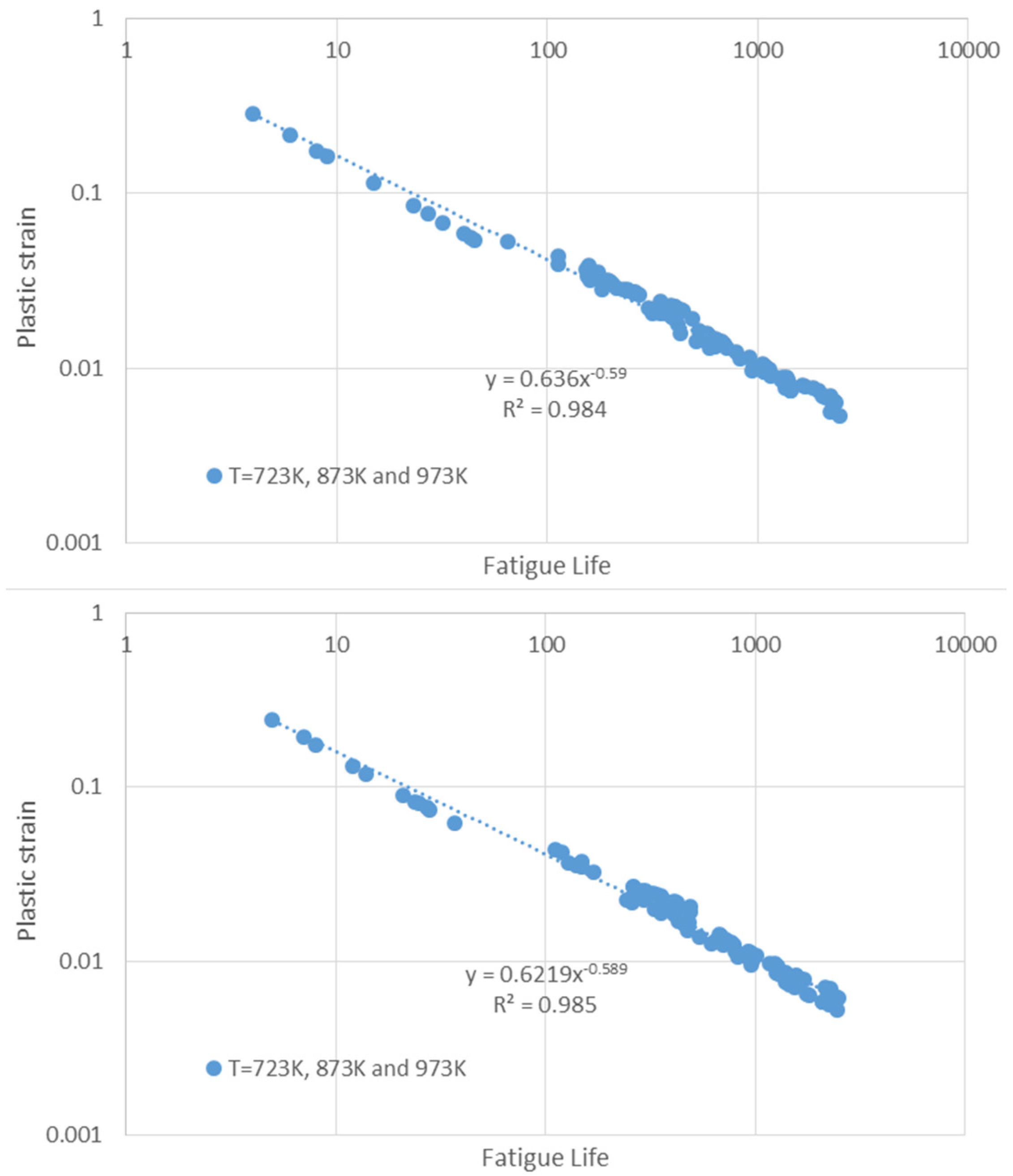
The fatigue life, temperature and strain rate are defined as random variables, and then 100 random creep-fatigue data points (plastic strain vs. fatigue life) were derived from [25] and the Coffin-Manson equation. These random data then were transformed into a reference condition through Equation (16). The transformation of 10 sets of random data (1000 data points) shows that these creep-fatigue data can collapse into almost one straight line at log-log scale (two of them are shown in Figure 8) with the quality of fit R² = 0.975–0.985. This transformation based on random data has further verified the unified equation, ${\mathsf{\epsilon }}_p=C_{0}c\left(T,t,{\mathsf{\epsilon }}_p\right)N^{-{\mathsf{\beta }}_0}$ and the form of creep function c (T, t, ε_p).

5.4. The Initial Proposal of Creep-Fatigue-Equation-Based Temperature Modified Coffin-Manson Equation

Frequency modified Coffin-Manson equation can be expressed as Equation (36) [34]:

$$\mathrm{∆}{\mathsf{\epsilon }}_p=C_0{\left[N_f{\nu }^{k-1}\right]}^m$$

(36)

where $\nu$ is the frequency, and k and m are the constant determined by experiments. Comparing this equation with the conventional Coffin-Manson equation (Equation (2)), the $N_f{\nu }^{k-1}$ can be defined as the frequency modified fatigue life. Similarly, comparing the unified creep-fatigue equations (Equations (14) and (17)) with the conventional Coffin-Manson equation (Equation (2)), ${\left[c\left(T,t,{\mathsf{\epsilon }}_p\right)\right]}^{-1/{\mathsf{\beta }}_0}N$ and ${\left[c\left(T,t\right)\right]}^{-1/{\mathsf{\beta }}_{0}b\left(T,t\right)}N$ can be defined as the temperature-frequency modified fatigue life (creep-fatigue life). If we get rid of frequency effect from the unified creep-fatigue equations, the creep-fatigue life ($N_{f-\mathrm{creep}+\mathrm{fatigue}}$) can be transformed to temperature modified fatigue life ($N_{f-\mathrm{temp}}$) through Equation (37), then the temperature modified Coffin-Manson equation could be developed through this transformation.

$$N_{f-\mathrm{temp}}=N_{f-\mathrm{creep}+\mathrm{fatigue}}·{\nu }^{k-1}$$

(37)

Because c₁ function in the strain-form unified creep-fatigue equation related to time-temperature relation, it is difficult to remove the frequency effect from this function. Therefore, the power-law unified creep-fatigue equation is used to develop the temperature modified Coffin-Manson equation (Equation (38)) through removing the frequency-related items and transforming creep-fatigue life to temperature modified fatigue life.

$${\mathsf{\epsilon }}_p=C_0\left[1-c_1\left(T-T_{\mathrm{ref}}\right)\right]{N_{f-\mathrm{temp}}}^{-{\mathsf{\beta }}_0\left[1-b_1\left(T-T_{\mathrm{ref}}\right)\right]}$$

(38)

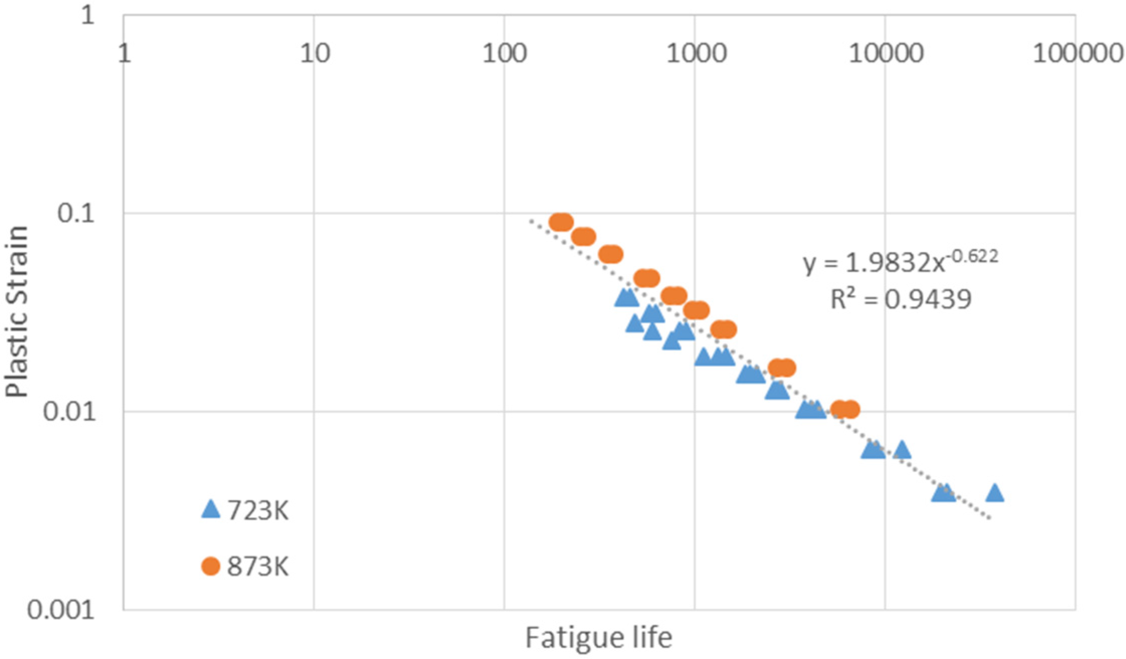
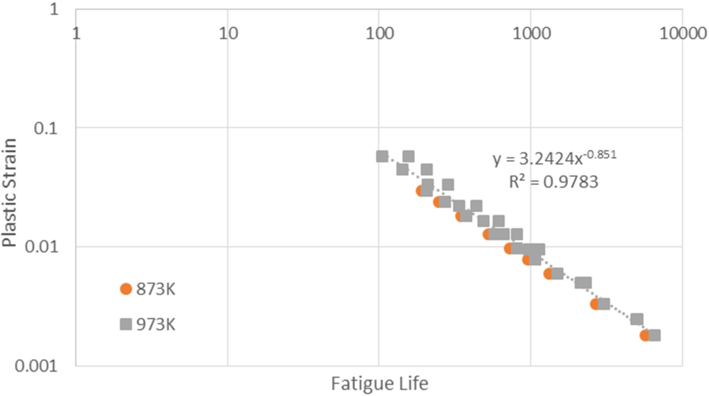
Based on the creep-fatigue data [25], the coefficients of this equation are evaluated (shown in

Table 1. The coefficients of Equation (38).

Temperature Regimes	${\mathit{C}}_0$	${\mathit{c}}_1$	${\mathsf{\beta }}_0$	${\mathit{b}}_1$	k
723 K–873 K	1.997	0.002955	0.62375	−0.000309	723 K: 0.728 873 K: 0.758
873 K–973 K	2.452	0.002668	0.80713	0.00088	873 K: 0.758 973 K: 0.873

). Then, using the coefficient shown in Table 1, the generated raw fatigue data (ε_p–N) obtained from [25] (T = 723 K, 873 K and 973 K) are transformed to the reference condition (ε_p,ref–N) through Equation (16). The transformed data at “723 K and 873 K”, and “873 K and 973 K” are plotted in Figure 9 and Figure 10 respectively.

Figure 9 and Figure 10 show that the creep-fatigue data below 873 K and above 873 K can be collapsed into power-law curves of ${\mathsf{\epsilon }}_{p,\mathrm{ref}}=1.9832N^{-0.622}$ with the quality of fit as R² = 0.9439 and ${\mathsf{\epsilon }}_{p,\mathrm{ref}}=3.2424N^{-0.851}$ with the quality of fit as R² = 0.9783 respectively. The errors between fatigue life from experiments and creep-fatigue equation for these two temperature regimes are 0.814 and 0.294. This transformation has verified the creep-fatigue-equation-based temperature modified Coffin-Manson equation.

5.5. Application and Future Research

The results have provided a derivation of the equations and the methods for determining the coefficients. While this may appear mathematically complex, it is a necessary feature of the work as it provides reproducibility and assists other researchers in applying and adapting the work.

The implications for practitioners, e.g., nuclear industry, are given in Section 4.3.3 and Section 4.4.3, using the two forms of the unified creep-fatigue equation. The equations are provided for stainless steel 316 and encapsulate the data for multiple temperatures, fatigue life, and plastic strain. In application, the equation might be used to determine fatigue life for given conditions (plastic strain, temperature and cycle time), or to determine acceptable plastic strain for a given life and other conditions.

6. Conclusions

The following major results were obtained:

(1) The strain-form unified creep-fatigue equation: ${\mathsf{\epsilon }}_p=C_{0}c\left(T,t,{\mathsf{\epsilon }}_p\right)N^{-{\mathsf{\beta }}_0}$ and power-law form: ${\mathsf{\epsilon }}_p=C_{0}c\left(T,t\right)N^{-{\mathsf{\beta }}_{0}b\left(T,t\right)}$ have been verified on stainless steel 316, and the methods of extracting the fatigue and the creep coefficients by limited creep-fatigue tests and creep rupture tests have been presented. The equations are efficient as they represent a whole range of conditions, in contrast to some other formulations which have to be calibrated separately for each set of environmental conditions.

(2) A moderating factor is introduced into the unified creep-fatigue equation to compress the amplitude of cyclic stress, and leads to a more reasonable result than the situation without moderating factor.

(3) The reliability of this unified creep-fatigue equation is verified through random variables.

(4) The creep-fatigue equation-based, temperature-modified Coffin-Manson equation is proposed, and this equation is validated through transforming raw data to the reference condition.

(5) However, there is a potential limitation. For the materials whose fatigue behaviour is strongly influenced by heat treatment, the coefficients obtained from one specific material condition cannot be used to predict the fatigue life of the same material at material conditions. This is identified as an area for future development of the theory.

References

- Holmström, S.; Pohja, R.; Nurmela, A.; Moilanen, P.; Auerkari, P. Creep and creep-fatigue behaviour of 316 stainless steel. Procedia Eng. 2013, 55, 160–164. [Google Scholar] [CrossRef]
- Basquin, O. The Exponential Law of Endurance Tests. Am. Soc. Test. Mater. Proc. 1910, 10, 625–630. [Google Scholar]
- Coffin, L.F., Jr. A Study of the Effects of Cyclic Thermal Stresses on a Ductile Metal; Knolls Atomic Power Lab.: Niskayuna, NY, USA, 1953. [Google Scholar]
- Manson, S.S. Behavior of Materials under Conditions of Thermal Stress; National Advisory Committee for Aeronautics: Cleveland, OH, USA, 1954.
- Feltner, C.E.; Morrow, J.D. Microplastic strain hysteresis energy as a criterion for fatigue fracture. J. Basic Eng. 1961, 83, 15–22. [Google Scholar] [CrossRef]
- Morrow, J. Cyclic plastic strain energy and fatigue of metals. In Internal Friction, Damping, and Cyclic Plasticity; ASTM International: West Conshohocken, PA, USA, 1965. [Google Scholar]
- Dowling, N.E. Mechanical Behavior of Materials: Engineering Methods for Deformation, Fracture, and Fatigue; Prentice Hall: Upper Saddle River, NJ, USA, 1993. [Google Scholar]
- Ramberg, W.; Osgood, W.R. Description of Stress-Strain Curves by Three Parameters; National Advisory Committee for Aeronautics: Cleveland, OH, USA, 1943.
- Palmgren, A. Die lebensdauer von kugellagern. ZVDI 1924, 68, 339–341. [Google Scholar]
- Miner, M.A. Cumulative damage in fatigue. J. Appl. Mech. 1945, 12, 159–164. [Google Scholar]
- Chopra, O.K. Environmental Effects on Fatigue Crack Initiation in Piping and Pressure Vessel Steels; Argonne National Lab.: Argonne, IL, USA, 2000.
- Gosselin, S.R.; Deardorff, A.F.; Peltola, D.W. Fatigue assessments in operating nuclear power plants. In Changing Priorities of Codes and Standards: Failure, Fatigue, and Creep. Pvp-vol. 286; American Society of Mechanical Engineers: New York, NY, USA, 1994. [Google Scholar]
- Rodabaugh, E. Comparisons of Asme-Code Fatigue-Evaluation Methods for Nuclear Class 1 Piping with Class 2 or 3 Piping; Rodabaugh (EC) and Associates: Hilliard, OH, USA, 1983. [Google Scholar]
- Rudolph, J.; Heinz, B.; Jouan, B.; Bergholz, S. Areva Fatigue Concept—A Three Stage Approach to the Fatigue Assessment of Power Plant Components; INTECH Open Access Publisher: Rijeka, Croatia, 2012. [Google Scholar]
- Zhu, Y.; Li, X.; Wang, C.; Gao, R. A new creep-fatigue life model of lead-free solder joint. Microelectron. Reliab. 2015, 55, 1097–1100. [Google Scholar] [CrossRef]
- Richart, F.; Newmark, N. An Hypothesis for the Determination of Cumulative Damage in Fatigue; Selected Papers By Nathan M. Newmark@ sCivil Engineering Classics; ASCE: Reston, VA, USA, 1948; pp. 279–312. [Google Scholar]
- Manson, S. Interfaces between fatigue, creep, and fracture. Int. J. Fract. Mech. 1966, 2, 327–363. [Google Scholar] [CrossRef]
- Gosselin, S. Fatigue Crack Flaw Tolerance in Nuclear Power Plant Piping: A Basis for Improvements to ASME Code Section XI Appendix L; US Nuclear Regulatory Commission, Office of Nuclear Regulatory Research, Division of Fuel, Engineering and Radiological Research: Washington, DC, USA, 2007.
- Rudolph, J.; Bergholz, S.; Willuweit, A.; Vormwald, M.; Bauerbach, K. Methods of detailed thermal fatigue evaluation of nuclear power plant components. Mater. Werkst. 2011, 42, 1082–1092. [Google Scholar] [CrossRef]
- Ainsworth, R.; Ruggles, M.; Takahashi, Y. Flaw assessment procedure for high-temperature reactor components. J. Press. Vessel Technol. 1992, 114, 166–170. [Google Scholar] [CrossRef]
- Paris, P.; Erdogan, F. A critical analysis of crack propagation laws. J. Basic Eng. 1963, 85, 528–533. [Google Scholar] [CrossRef]
- Wong, E.; Mai, Y.-W. A unified equation for creep-fatigue. Int. J. Fatigue 2014, 68, 186–194. [Google Scholar] [CrossRef]
- Shi, X.; Pang, H.; Zhou, W.; Wang, Z. Low cycle fatigue analysis of temperature and frequency effects in eutectic solder alloy. Int. J. Fatigue 2000, 22, 217–228. [Google Scholar] [CrossRef]
- Wong, E.H.; Liu, D. The unified equations for creep-fatigue—Deriving creep function from creep-rupture parameters. Int. J. Fatigue submitted for publication. 2016. [Google Scholar]
- Kanazawa, K.; Yoshida, S. Effect of Temperature and Strain Rate on the High Temperature Low-Cycle Fatigue Behavior of Austenitic Stainless Steels. In Proceedings of the International Conference on Creep and Fatigue in Elevated Temperature Applications, Philadelphia, PA, USA, 23–27 September 1973; Institution of Mechanical Engineers: London, UK, 1975; Volume 1. [Google Scholar]
- High Temperature Characteristics of Stainless Steels. Available online: https://www.nickelinstitute.org/~/Media/Files/TechnicalLiterature/High_TemperatureCharacteristicsofStainlessSteel_9004_.pdf (accessed on 8 September 2016).
- Orr, R.L.; Sherby, O.D.; Dorn, J.E. Correlations of Rupture Data for Metals at Elevated Temperatures; DTIC Document: Fort Belvoir, VA, USA, 1953. [Google Scholar]
- Larson, F.R.; Miller, J. A Time-Temperature Relationship for Rupture and Creep Stresses; Trans ASME: New York, NY, USA, 1952; pp. 765–771. [Google Scholar]
- Manson, S.; Haferd, A. A Linear Time-Temperature Relation for Extrapolation of Creep and Stress Rupture Data; NaCA TN 2890; Lewis Flight Propulsion Laboratory Cleveland: Cleveland, OH, USA, 1953.
- Penny, R.K.; Mariott, D.L. Design for Creep; Chapman & Hall: London, UK, 1995. [Google Scholar]
- Engineering Virtual Organization for CyberDesign. 316 Stainless Steel. Available online: https://icme.hpc.msstate.edu/mediawiki/index.php/316_Stainless_Steel (accessed on 6 September 2016).
- Halford, G. Cyclic creep-rupture behavior of three high-temperature alloys. Metall. Trans. 1972, 3, 2247–2256. [Google Scholar] [CrossRef]
- Jaske, C.; Mindlin, H.; Perrin, J. Development of Elevated Temperature Fatigue Design Information for Type 316 Stainless Steel; Battelle Columbus Labs.: Columbus, OH, USA, 1975. [Google Scholar]
- Coffin, L., Jr. Predictive Parameters and Their Application to High Temperature, Low Cycle Fatigue; ICF2: Brighton, UK, 1969. [Google Scholar]
Figure 1.
The relation between pure fatigue and pure creep.
Figure 3.
Transformed εp,ref-N data of stainless steel 316 using Equation (14) with creep function c (T, t, εp).
Figure 4.
Transformed εp,ref–N data (below 873 K) of stainless steel 316 using Equation (17) with functions c (T, t) and b (T, t).
Figure 5.
Transformed εp,ref–N data (above 873 K) of stainless steel 316 using Equation (17) with functions c (T, t) and b (T, t).
Figure 6.
Transformed εp,ref–N data of stainless steel 316 using Equation (14) with creep function c (T, t, εp) and moderating factor.
Figure 7.
Transformed εp,ref–N data of quenched and aged stainless steel 316 using Equation (14) with creep function c (T, t, εp).
Figure 8.
Transformed εp,ref–N data of stainless steel 316 using Equation (14) with creep function c (T, t, εp) and random variables. Data shown are for two of ten sets, as evidence of a consistent transformation process.
Figure 9.
Transformed εp,ref–N data (below 873 K) of stainless steel 316 using Equation (17).
Figure 10.
Transformed εp,ref–N data (above 873 K) of stainless steel 316 using Equation (17).