Article

A Phase Field Model for Rate-Dependent Ductile Fracture

1
Department of Mechanical Engineering, Behbahan Khatam Alanbia University of Technology, Khuzestan 63616-47189, Iran
2
Department of Civil Engineering, Semnan University, Semnan 35131-19111, Iran
3
Department of Civil Engineering, College of Engineering, University of Babylon, Babylon 51002, Iraq
*
Author to whom correspondence should be addressed.
Metals 2017, 7(5), 180; https://doi.org/10.3390/met7050180
Submission received: 17 April 2017 / Revised: 29 April 2017 / Accepted: 5 May 2017 / Published: 17 May 2017
(This article belongs to the Special Issue Microstructure based Modeling of Metallic Materials)

Abstract

:
In this study, a phase field viscoplastic model is proposed to model the influence of the loading rate on the ductile fracture, as one of the main causes of metallic alloys’ failure. To this aim, the effects of the phase field are incorporated in the Peric’s viscoplastic model; the model can efficiently be converted to a standard rate-independent model. The novel aspects of this work include: Describing a coupling between rate-dependent plasticity and phase field formulation by defining an energy function that contains the energy dissipation caused by plastic deformation as well as the fracture process and elastic energy. In addition, the equations required to develop the numerical solution are presented. The governing equations are determined by a minimization principle that results in balance laws for the coupled displacement-phase field problem. Furthermore, an implicit integration algorithm for a viscoplasticity model coupled with a phase field is presented for a three-dimensional stress state. The proposed algorithm can be utilized for different constitutive models of rate-dependent and rate-independent plasticity models coupled with fracture by changing the definition of the plastic multiplier. In addition, to control the influence of the plastic deformation and its work on the crack propagation, a threshold variable is defined in the model. Finally, using the proposed model, the influence of the loading rate on the responses of the different specimens in one-dimensional and multi-dimensional cases is investigated and the accuracy of the results was verified by comparing them with existing experimental and numerical results. The obtained result proves that the model can simulate the impact of the loading rate on the material response, and the gradual change of the fracture phase from ductile to brittle, caused by increasing the loading rate.

1. Introduction

It is widely accepted that the behavior of many materials, specifically metals, is naturally time-dependent. For instance, when the temperature is higher than one-third of the melting point, the metals’ behavior is significantly dependent on time. In such cases, the initiation of failure, hardening, and ductility is reliant on the loading rate. For many mechanical processes, such as metal-forming and the mechanics of fracture, it is crucial to consider the dependency of material behaviors to the loading rate. Creep is another example of a time-dependent mechanical behavior that usually occurs over a long period of time while the material is subjected to constant stress. Through the creep process, strain changes as a function of time. Stress relaxation is also a good example of time-dependent mechanical phenomena, in which a material is under a constant value of strain over a long period of time. In an experimental test of stress relaxation, the specimen is often deformed (with a constant strain) and stress gradually reduces as a function of time. Viscoplastic models usually simulate time-dependent behavior. Most of the viscoplastic models are categorized as either “Perzyna” or “Duvaut–Lions” models. In these models, stress can be increased beyond the yield stress of the rate-independent case and then can relax back to the yield level. In such models, yield stress is not dependent on the loading rate. Another method to simulate time-dependent processes is to consider the influence of the loading rate in yield stress and use the existing methods for the rate-independent models.
The simulation of crack nucleation and propagation through numerical simulations is of great importance for engineering design. The variational-based phase field method to fracture provides a valuable new tool for the numerical modeling of complex fracture processes. The phase-field-based methods to fracture are regularizing sharp crack discontinuities in continuum formulation. In this method, crack is indicated by a scalar field variable, which is also coupled to the material constitutive model to consider the change in material behavior between damaged and undamaged states. Moreover, the phase field model to fracture has no difficulty in simulating the cracks nucleation or the branching and merging of cracks. The quasi-static brittle fracture of phase field and its applications have been developed by Kuhn et al. [1], Miehe et al. [2,3,4], Hofacker and Miehe [5], May et al. [6], Msekh et al. [7,8], Liu et al. [9], Borden et al. [10], Borden [11], and Ambati et al. [12].
Recently, the phase field application has been extended to the rate-independent ductile fracture region. Ambati et al. [13,14] developed a phase field model for the ductile fracture of solids in the quasi-static region. In their model, the classical definition of the phase field degradation function is changed. They introduced a coupling between the phase field degradation function and the plastic strain to control the role of plastic deformation on the crack propagation. They also extended this model to the finite strain region and verified their results with the experimental investigation [15]. Duda et al. [16] formulated a phase field model of fracture in elastic-plastic solids under small strains assumption. They demonstrated that the phase field approach coupled with rate-independent plasticity is suitable to simulate the plastic deformations role during the surface separation phenomena observed in crack propagation problems. A variational-based approach for the phase field modeling of rate-independent ductile fracture in elastic-plastic solids at large strains has been proposed by Miehe et al. [17,18,19]. In their work, the phase field model of fracture was associated with a formulation of gradient plasticity. They demonstrated that finite element simulation of localized ductile fracture behaviors leads to pathological mesh dependencies in the post-critical range. The developed gradient-enhanced plasticity model is to regularize the ductile failure model. Hernandez and Markert [20] proposed a numerical approach in an elasto-plastic crystal plasticity model including a phase-field model adjusted to predict ductile fracture. The implemented model within the finite element context is used to simulate ductile fracture under quasi-static tensile loading. Some modifications to develop phase field models for fracture in rate-independent ductile materials are proposed by Borden et al. [21]. These modifications include a cubic degradation function, a method for measuring of stress triaxiality as a driving force of initiation and propagation of cracks, and a correction to an error in the configuration update of an elasto-plastic return-mapping algorithm for large deformation models. A phase field theory for modeling deformation and fracture of single crystals and polycrystals at finite strain has been developed by Clayton and Knop [22,23,24]. They considered anisotropy in crystal elastic responses and fracture properties in 3D finite element simulations [23]. They also suggested a phase field theory for coupled twinning and fracture in single crystal domains is developed [24]. Clayton and Knop [25] proposed a phase field theory by considering both fracture and deformation twinning behaviors in crystalline solid in order to address both cleavage fracture and deformation twinning phenomena. Moreover, Areias et al. [26,27] presented the phase field model in finite strain contexts for elastic and elasto-plastic constitutive laws of materials in shells and with coupled multi-field model using Cahn–Hilliard-type diffusion for electro-chemo-mechanics of lithium ion (Li-ion) batteries.
Application of the phase field approach to rate-dependent ductile fracture is very limited. Recently, Shanthraj et al. [28] proposed a phase field method for brittle fracture for a finite strain elasto-viscoplastic material utilizing a novel obstacle phase field energy model. They used the model to simulate the localization of damage on a defined family of crystallographic planes and characteristic of cleavage fracture in metals [29].
Most of the phase field ductile fracture models do not consider the influence of the loading rate on the material behavior. In this study, a phase field model of rate-dependent ductile fracture is developed. For this end, a phase field degradation function for the material stiffness and yield stress is introduced in a viscoplastic model. In this model, the phase field driving force is calculated based on the plastic work and the elastic energy of the body. Furthermore, a plastic work threshold is defined to control the initiation of the influence of the plastic deformation. The solution scheme of displacement field and phase field equations using finite element method (FEM) is presented and the integration method of proposed model, as a basis of finite element solutions is described. The ability of the proposed model to estimate rate-dependent ductile fracture of different materials is evaluated. To this aim, benchmarks tests are used for both rate-dependent and rate-independent cases. Finally, the influence of various material parameters is examined, using one-dimension and multi-dimension simulations. According to these simulations, the ability of the proposed model in different loading rates is investigated using the obtained results, quantitatively and qualitatively.

2. Formulation

2.1. Viscoplastic Model

Similar to the models that are independent of loading rate, the first step is to separate strain ( ε ) into its elastic ( ε e ) and plastic ( ε p ) components, under small strain conditions:
ε = ε e   +   ε p .
Assuming that the behavior of the material is isotropic in elastic phase, the constitutive behavior of the material can be defined as:
σ = D e   :   ε e ,
where σ is the so-called Cauchy stress tensor. In addition, the sign (:) indicates double dot product operation between two tensors and D e is the isotropic fourth-order elastic stiffness tensor for undamaged materials,
D e = 2 G I d   +   K I I ,
in which the sign ( ) indicates tensor product operation between two tensors, G and K are, respectively, the shear and bulk moduli, I the second-order identity tensor, I d = I s 1 3 I I the fourth-order deviatoric projection tensor and I s is the fourth-order symmetric identity tensor. Yield function for this material is defined based on the von Mises stress, similar to the Mises-based rate-independent plasticity material model:
f ( σ )   =   σ e ( s ( σ ) )     σ y     0 ,
where σ y is the yield stress, σ e = 3 2 s : s is the effective stress and s is the deviatoric stress, which is defined as:
s   =   σ     1 3 σ   :   I .
It is apparent that the yield function is rate-independent. However, the main difference between this model and the classical rate-independent plasticity model is the definition of the plastic flow rule and accordingly the definition of the time derivative of the plastic strain:
ε ˙ p   =   γ ˙ N ,
where γ is the plastic multiplier and N is the associated flow vector:
N   =   f σ   =   3 2 s s   ,
in which   defines the Euclidean norm of tensors. The main difference between viscoplastic models is the definition of γ ˙ , which defines the change of the plastic strain as a function of stress. Perzyna’s model [30], which is widely used in numerical models, defines the plastic multiplier as below:
γ ˙ = { 1 μ [ σ e σ y 1 ] 1 / ϵ    i f   f ( σ ) 0 0    i f   f ( σ ) < 0 .
In this study, Peric’s model [31] is used, in which the plastic multiplier is defined as:
γ ˙ = { 1 μ [ ( σ e σ y ) 1 / ϵ 1 ]    i f   f ( σ ) 0 0    i f   f ( σ ) < 0 .
In Equation (9), μ and ϵ are the material constants. μ is the viscosity-related parameter, whose dimension is time, and ϵ is the non-dimensional rate sensitivity parameter. According to the Peric’s definition, if ϵ 0 or μ 0 , the model converts to the classical rate-independent model. Peric has proved that in Perzyna’s model, if the effect of the loading rate is not considered with ϵ 0 , the model will not have the ability to produce accurate one dimensional stress-strain behavior of the material, in a rate-independent case. However, when μ 0 , the results of both models coincide with the standard rate-independent model [32]. The isotropic hardening that determines the size of the yield surface can be incorporated into the model simply by assuming that
σ y = σ y ( ε ¯ p ) ,
where ε ¯ p is the von Mises equivalent or accumulated plastic strain, defined as
ε ¯ p = 0 t 2 3 ε ˙ p d t .

2.2. Phase Field Approximation of a Crack

The Griffith fracture theory reaches its limits when it uses to predict crack path, nucleation of new cracks and complicated crack behavior during kinking and branching. A variational based formulation can solve these problems. Phase field approach is a regularized version of the variational formulation. The main advantage of the phase field approach is that cracks are no longer depended on the geometry. This provides a powerful tool to simulate complex crack initiation, propagation, kinking and branching. In addition, the finite element implementation becomes straightforward. In the phase field fracture model, the main idea is to evaluate a sharp discontinuity Γ by a smeared surface Γ l [6]. For this end, an auxiliary field, called order phase field variable, is introduced to represent the crack. In other hand, the crack discontinuity is described by a scalar field d [ 0 ,   1 ] , the phase field variable, where the undamaged state defined by d = 0 and the fully-cracked state of the material point is described by d = 1. The defined scalar field is similar to the damage mechanics concept. As demonstrated by Miehe et al. [2], Γ can be approximated by Γ l as follows:
Γ l =   γ l d V =   1 2 l ( d 2 + l 2 d , x 2 ) d V = 0 ,
where a comma defines differentiation, the function γ l can be considered as the crack surface density. Definition of the crack surface density function γ l can be expanded to a multi-dimensional case as:
γ l = 1 2 l ( d 2 + l 2 d , i d , i ) .
The three-dimensional form of Equation (13) is identical to the damage-based implicit gradient-enhanced model [33]; however, they have different interpretations. In addition, the gradient-enhanced models are usually used to introduce an internal length scale into the formulation in order to remove mesh sensitivity in finite element simulations [34,35,36]. However, this makes gradient-enhanced damage formulations less suitable to simulate a sharp crack [37].

2.3. Phase Field Model for Brittle Fracture

The total energy of a brittle solid material with a discrete crack is a function of both displacement field u and fracture phase field d and can be written as:
E ( u ,   d ) =   ψ ( ε , d ) d V =   g c γ l d V +   ψ e l d V ,
in which g c is the Griffith-type fracture energy which is defined as the amount of energy required to produce a unit area of fracture surface. In Equation (14), the first term is the fracture energy caused by crack and the second term is the elastic energy. When the total energy is minimized with respect to admissible phase field variable and displacement fields with a determined boundary conditions, the regularized formulation of the crack evolution can be extracted. Using the assumption of isotropic degradation of stored bulk energy caused by fracture; the elastic energy density can be defined as:
ψ e l ( ε , d ) = [ g ( d ) + k ] ψ 0 e l ( ε ) ,
where ψ 0 e l = 1 2 ε : D e : ε is the standard elastic energy for undamaged solids. The small positive dimensionless parameter 0 < k 1 is a stabilizer parameter introduced to avoid numerical difficulties at a fully-damaged state ( d = 1 ). A small remaining elastic energy density k ψ 0 e l ( ε ) keeps the algebraic well-posed condition for the partly damaged material points. In Equation (15), the degradation function g ( d ) is a monotonically decreasing function introduced to reduce the material stiffness due to damage. In this paper, a quadratic function that has the abovementioned properties is used:
g ( d ) = ( 1 d ) 2 .
Readers are referred to [2,6] for more descriptions. In addition, the effect of the quadratic and cubic degradation functions on the rate-independent ductile phase field model has been investigated by Borden et al. [21]. By substituting Equations (15) and (16) into Equation (14), the total energy functional can be derived as:
E ( u ,   d ) =   g c γ l d V +   [ ( 1 d ) 2 + k ] ψ 0 e l ( ε ) d V .
The total energy functional E ( u ,   d ) must be minimized for a determined equilibrium state:
δ E ( u ,   d ) = E ( u ,   d ) ε δ ε + E ( u ,   d ) d δ d + E ( u ,   d ) d ˙ δ d ˙ = 0 .
The regularized formulation of the crack propagation is determined using the minimization under given boundary conditions. For the minimization, the variation of the total energy functional must be zero for all admissible values of δ ε and δ d . According to this condition, the strong form of system of equations for the displacement field and the phase field can be derived as:
𝛻 · σ = 0 ,
g c l ( d l 2 d ) = 2 ( 1 d ) ψ 0 e l ( ε ) .
The above system of equations is subjected to the following boundary conditions:
σ · n = t N   at   t ,
𝛻 d · n = 0   at   ,
in which n is the unit normal vector to the surface and t N the surface traction vector. The constitutive equation for the stress can be obtained as:
σ = ε ψ = ε ψ e l = [ ( 1 d ) 2 + k ] D e : ε .

2.4. Phase Field Model for Rate-Dependent Ductile Fracture

The influence of the plastic work should be taken into account while defining the stored energy if the plastic deformation during the process of crack propagation should be considered. Generally, it is necessary to consider an inelastic strain so as to use the elastic strain instead of the total strain. Then, the influence of the plastic work will be applied on the driving force to control the crack propagation. For instance, in a thermomechanical phase field model, the thermal strain is subtracted from the total strain to find the elastic strain. In ductile phase field models, based on the same definition of stored energy, the elastic strain is used instead of the total strain ( ε e = ε ε p ) and the effect of the plastic work will be taken into account:
E ( u ,   d ) =   g c γ l d V +   g ( d ) { β e ψ 0 e l ( ε ε p ) + β p ψ p ( α ) } d V ,
in which 〈 〉 is the Macauley bracket that is defined as,
x = { x   i f   x 0   0   i f   x < 0
α is a hardening internal variable, ψ p is the effective plastic work contribution to the energy. In addition, β e [ 0 ,   1 ] and β p [ 0 ,   1 ] are introduced here to weight the contribution of the elastic strain energy and plastic work to crack growth. The elastic energy is used to define the stress-strain constitutive equation and the contribution of the plastic driving force of the undamaged material. Furthermore, the effective plastic work is used to extract a hardening law, characterizing the evolution of the yield limit of the undamaged material. The effective plastic work is computed based on the following rate form definition:
ψ ˙ p = γ ˙ s .
In the proposed viscoplastic model, hardening is considered to be isotropic and the hardening internal variable is equal to the equivalent plastic strain ( ε ¯ p ). In Equation (24), the degradation function is multiplied to the effective plastic work and produces a coupling between fracture and plasticity. According to these assumptions, the constitutive equation for the stress can be obtained similarly to the brittle model using the elastic strain definition as
σ = ε e ψ e l = g ( d ) D e : ( ε ε p ) .
Analogously to the phase field model of brittle fracture, for the phase field model of ductile fracture the two coupled balance equations can be obtained as
𝛻 · σ = 0 ,
g c l ( d l 2 d ) = 2 ( 1 d ) [ β e ψ 0 e l ( ε ε p ) + β p ψ p ( α ) W 0 ] ,
where W 0 is a plastic work threshold. As explained by Borden et al. [21], this variable provides a mechanism to control the point at which plastic deformation contributes to the phase field driving force. The right hand side term in Equation (29) is the phase field driving force for ductile fracture. However, this definition may lead to a reversible phase field formulation, in which the phase field variable is free to evolve based on the loading history. In order to overcome this problem, the damage like formulation introduced by Miehe et al. [2] is used here. According to this, a history parameter is defined as
: = β e max [ 0 , t ] ( ψ 0 e l ( ε ε p ) ) + β p ψ p ( α ) W 0 .
Since the effective plastic work, ψ p ( α ) , is monotonically increasing, in the above definition the constraint is only introduced for the elastic strain energy to enforce irreversible crack growth. Substituting Equation (30) into (29) yields
g c l ( d l 2 d ) = 2 ( 1 d ) .
A primal-dual active set strategy has been proposed by Heister et al. [38] to enforce crack irreversibility as a constraint. An alternative approach has been suggested by Bourdin et al. [39], in which Dirichlet boundary conditions are imposed on the phase field variable.

2.5. Integration Algorithm

An integration algorithm for the proposed viscoplastic model with phase field extension is presented in this section. The proposed algorithm is analogous to that proposed by Neto et al. [32] for the purely viscoplastic model without fracture. The algorithm comprises the standard elastic predictor and the viscoplastic corrector. In the elastic predictor step, it is assumed that the material has an elastic behavior within the time interval [tn, tn+1]. Based on this assumption, the elastic trial state can be computed as
ε e   trial = ε n e + ε ,
ε p   trial = ε n p ,
ε ¯ p   trial = ε ¯ n p ,
σ trial = g ( d ) D e : ε e   trial ,
where, for notational convenience, the subscript n + 1 is omitted from the trial and updated values throughout this paper. Based on Equation (35), the degradation function reduces the material stiffness. If, based on the trial state, the condition
f ( σ trial ) = σ e trial ( s trial ) g ( d ) σ y ( ε ¯ p   trial ) 0
becomes true, then the current increment is purely elastic and the quantities at the end of current time interval are equal to the values computed at the elastic prediction state. Otherwise, the viscoplastic return mapping procedure must be considered to correct the predicted values. Equation (33) implies that the yield stress is reduced by the degradation function for a damaged material point. The von Mises yield function is pressure-independent so that the associated flow vector defined by Equation (7) is a function of the deviatoric stress. Therefore, the hydrostatic stress is independent of the viscoplastic flow and its value is constant during the viscoplastic return mapping procedure. Hence, the stress update relation can be split as
s = s trial 2 g ( d ) G γ 3 2 s s   ,
p = p trial ,
in which γ is the incremental value of plastic multiplier and can be calculated as
γ = t μ [ ( σ e g ( d ) σ y ( ε ¯ p ) ) 1 / ϵ 1 ] ,
where t is the time increment and ε ¯ p = ε ¯ n p + γ . In addition,
p trial = g ( d ) K ε v e   trial ,
s trial = 2 g ( d ) G ε d e   trial ,
in which ε v e   trial and ε d e   trial are the volumetric and deviatoric parts of the elastic trial strain. By rearranging the deviatoric stress update formula, we obtain
( 1 + 3 2 2 g ( d ) G γ s ) s = s trial ,
which implies that the trial and updated deviatoric stresses are co-linear and
s s = s trial s trial .
By substituting the above equation into Equation (39), it can be simplified to,
s = ( 1 3 2 2 g ( d ) G γ s trial ) s trial = ( 1 3 g ( d ) G γ σ e trial ) s trial .
Application of the definition of the von Mises effective stress to the above relation results in:
σ e   =   σ e trial 3 g ( d ) G γ .
By substituting the above equation into Equation (39), after a straightforward rearrangement we obtain
( σ e trial 3 g ( d ) G γ ) ( t γ μ + t ) ϵ g ( d ) σ y ( ε ¯ n p + γ ) = 0 .
The above is a nonlinear scalar equation in which γ is the only unknown. This equation can be solved by the Newton–Raphson method. Then, with γ at hand, the state variables can be updated. The Integration algorithm for the proposed rate-dependent ductile fracture model is summarized as follows:
(1)
Elastic predictor:
ε ¯ p   trial = ε ¯ n p
ε e   trial = ε n e + ε
p trial = g ( d ) K ε v e   trial
s trial = 2 g ( d ) G ε d e   trial
(2)
Check for viscoplastic flow:
IF   σ e trial ( s trial ) g ( d ) σ y ( ε ¯ p   trial ) 0   THEN
Set   ( · ) n + 1 = ( · ) n + 1 trial
EXIT
ELSE
GO   TO   step   3
(3)
Viscoplastic return mapping. Solve return mapping equation for γ in iterative form:
R ( γ ) = ( σ e trial 3 g ( d ) G γ ) ( t γ μ + t ) ϵ g ( d ) σ y ( ε ¯ n p + γ ) = 0
γ k + 1 = γ k + R k ( γ R ) k .
(4)
By γ at hand, update state variables:
ε ¯ p = ε ¯ n p + γ
p = p trial ,   s = ( 1 3 g ( d ) G γ σ e trial ) s trial .
σ = s + p I
(5)
Exit

2.6. Finite Element Implementation

The finite element implementation of the initial boundary value problem is explained in this section. The starting point for the finite element implementation is converting the strong forms of the displacement equilibrium Equation (28) and the phase field system Equation (29) to a weak form. By integration, the displacement equilibrium Equation (28) over the domain is:
  δ u ( · σ ) = 0 .
By applying the divergence theorem, using the chain rule, and applying the boundary condition given by Equation (21), Equation (47) can be transferred to
  ( δ u ) T : σ   d V = ( δ u ) T t N   d S .
Using the same method as described for the previous field, multiplication of the strong form of the phase field Equation (31) by δ d followed by integration over the volume leads to
  δ d { g c l ( d l 2 d ) 2 ( 1 d ) }   d V = 0 .
Appling the phase field boundary conditions given by Equation (22) and the same approach as before, weak form of the phase field evaluation equation is obtained:
  { g c l ( δ d   d + ( 𝛻 δ d )   l 2 𝛻 d ) 2   δ d ( 1 d ) }   d V = 0 .
In order to solve the governing equations numerically, it is necessary to introduce a discretization of the domain:
u = N u u e ,   δ u = N u u e ,   ε = B u u e ,
d = N d d e ,   δ d = N d d e ,   𝛻 d e = B d d e ,
where N u and N d are the shape function matrices for the displacement field and phase field, and B u and B d are matrices containing derivatives of the shape functions N u and N d , respectively. By substituting the above discretization relations into the two-field system given by Equations (48) and (50) and after some modifications, the relations will change to
( δ u ) T   B u T σ   d V f i n t u ( δ u ) T   N u T t N   d S f e x t u = 0 ,
( δ d ) T [   { g c l ( N d T   N d + B d T   l 2 B d ) d 2   N d T ( 1 d ) }   d V ] f i n t d = 0 .
Finally, the system of equations can be shown as follows:
[ f i n t u f e x t u f i n t d ] = 0 .
The above nonlinear system of equation is solved using the well-known Newton–Raphson iterative scheme. To this end, the nonlinear system of Equation (55) must be linearized.

3. Results and Discussion

The details of the phase field model for rate-dependent ductile fracture are presented in the previous sections. The proposed model considers the influence of the loading rate on the crack propagation for ductile materials. The plastic work threshold variable is introduced for better control of the crack initiation caused by plastic deformation. Moreover, two β p and β e constants control the role of the plastic work and elastic energy in crack growth. In this section, using the proposed FEM, the ability of the modeling for rate-dependent behavior and crack propagation will be investigated. First, the influence of the different variables using one-dimension simulations will be evaluated. Afterward, two-dimensional and three-dimensional specimens are also simulated by which the potency of the model to simulate the fracture process in more complex cases can be assessed. All the simulations are solved by FEM with a displacement-controlled condition. In addition, all the one-dimensional simulations are solved using monolithically coupled solution technique in which the displacement field and phase field are simultaneously updated by the Newton–Raphson iterative solution. However, two-dimensional and three-dimensional simulations have been solved with a staggered method. In this method, at each step of solution, while the displacement field is constant, the phase field is updated. Afterward, while the new phase field is constant, the solution process will be performed for the displacement field in which stress and the other state variables such as the phase field driving force will be updated. The phase field fracture model needs fine mesh in the fracture area. Miehe et al. [3] demonstrated that for given values of the mesh size, a length scale parameter close to l 2   h is appropriate. Obviously, this condition is only necessary in areas close to the crack surface. The developed finite element code is based on deal.II open source software [40,41].

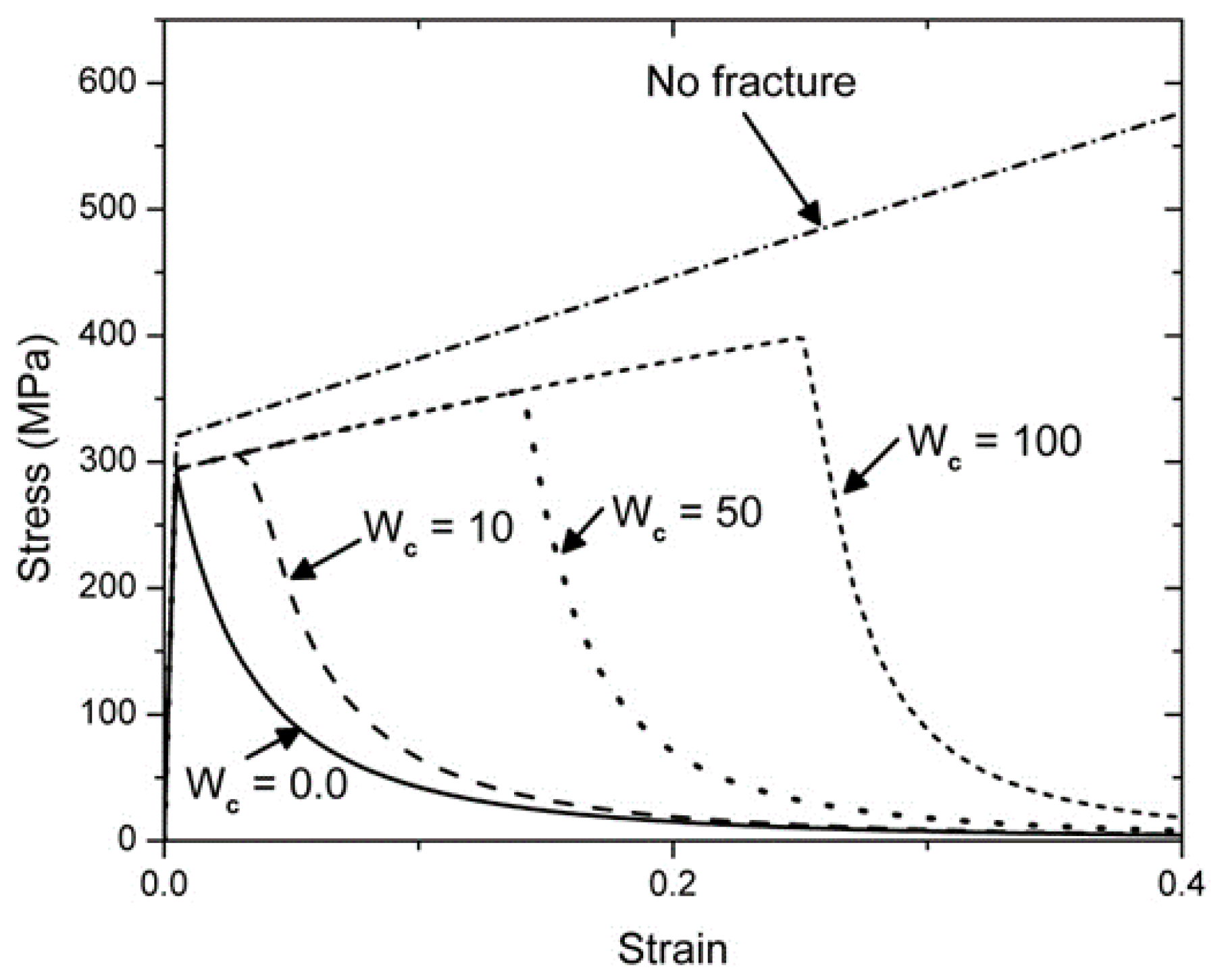
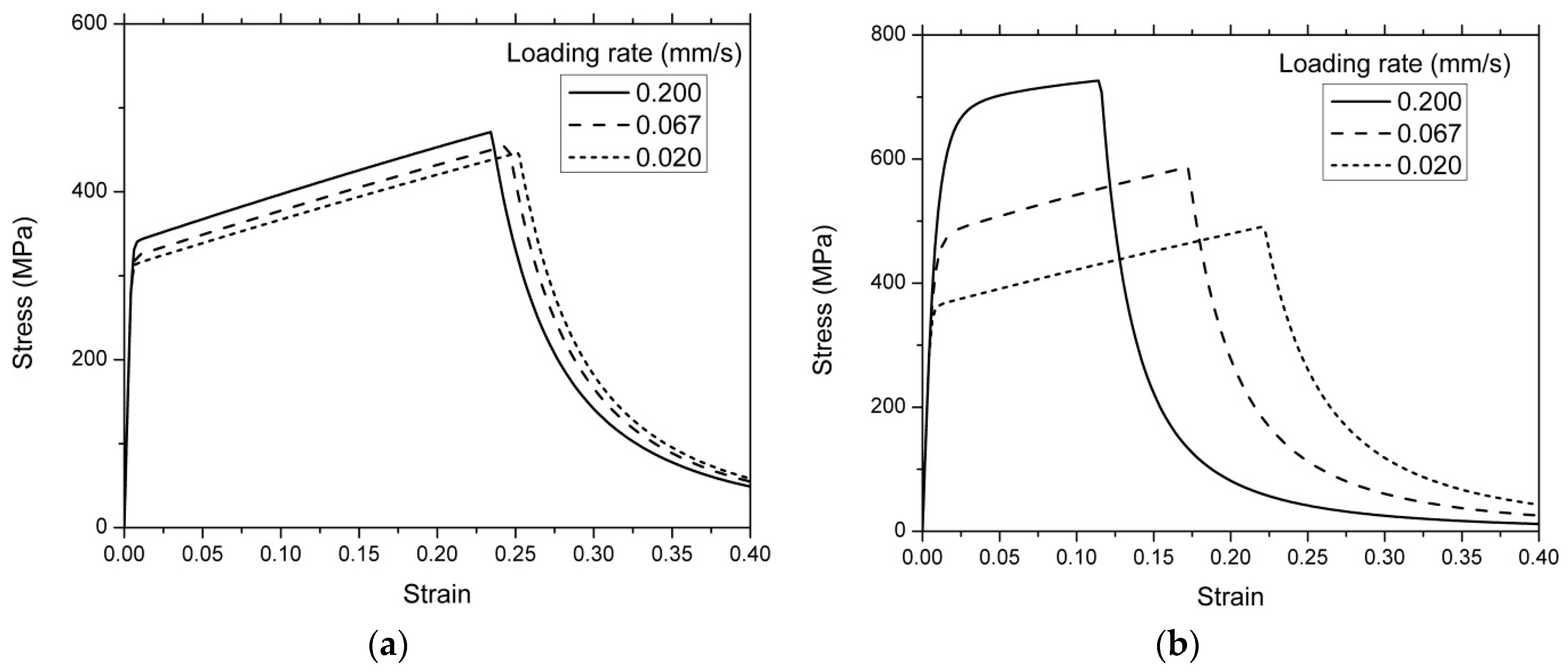
3.1. One-Dimensional Simulations

The impact of the different variables on the constitutive response of the proposed model is investigated using one-dimensional simulations. In these simulations, a bar element with two nodes and a uniform cross section area of 1 mm2 is used, in which each node has a one degree of freedom of displacement and one degree of freedom of phase field. Furthermore, the length scale parameter is chosen larger than the element size, so that deformation is homogeneous along the specimen. Table 1 shows the material properties that are used in one-dimensional simulations. In some cases, other properties are used to model the behavior of the intended materials, as will be mentioned later.
The first simulation is developed regardless the loading rate influence. To eliminate the rate effect, the viscosity or rate sensitivity parameters have to be zero. In this case using μ = 0 , the model is converted to a rate-independent phase field model for ductile fracture. In this simulation, the influence of the plastic work threshold on the response of the model is also investigated. The stress-strain response obtained from this simulation is compared with the stress-strain response of the standard J2-plasticity model without fracture (Figure 1). It is apparent that the plastic work threshold parameter is the controller of the ductile fracture initiation. It is also clear that in cases where the fracture is included, yield stress is slightly lower in comparison with the response of the cases without fracture. The main reason for such a difference is the influence of the elastic energy on the reduction of the yield level, while the equivalent plastic work has not met the value of the plastic work threshold. The results of this simulation are in a complete agreement with the results reported by Borden et al. [21]. This agreement verifies the accuracy of the finite element solution so as to show the ability of the model to convert to a classical rate-independent model.
In the second simulation, the influence of the loading rate and the rate sensitivity parameter on the response of the proposed model is investigated. In this simulation, all the parameters of the model are presented in Table 1. Compared to the previous simulation the value of the viscosity parameter is not zero ( μ = 10   s ). The achieved results from this simulation, which has been developed for low, moderate, and high loading rates, are demonstrated in Figure 2. Figure 2 shows the influence of the loading rate on the stress-strain response, in which the ductile fracture caused by the phase field degradation function is included. Moreover, to show the impact of the rate sensitivity parameter, two values ( ϵ = 1.0 and ϵ = 0.1 ) are considered. It can be seen that for a constant value of the rate sensitivity parameter, at a higher loading rate, the maximum stress increases while the fracture starts at a lower strain. In other hand, the material ductility reduces as the loading rate increases and the rate sensitivity parameter controls this effect.

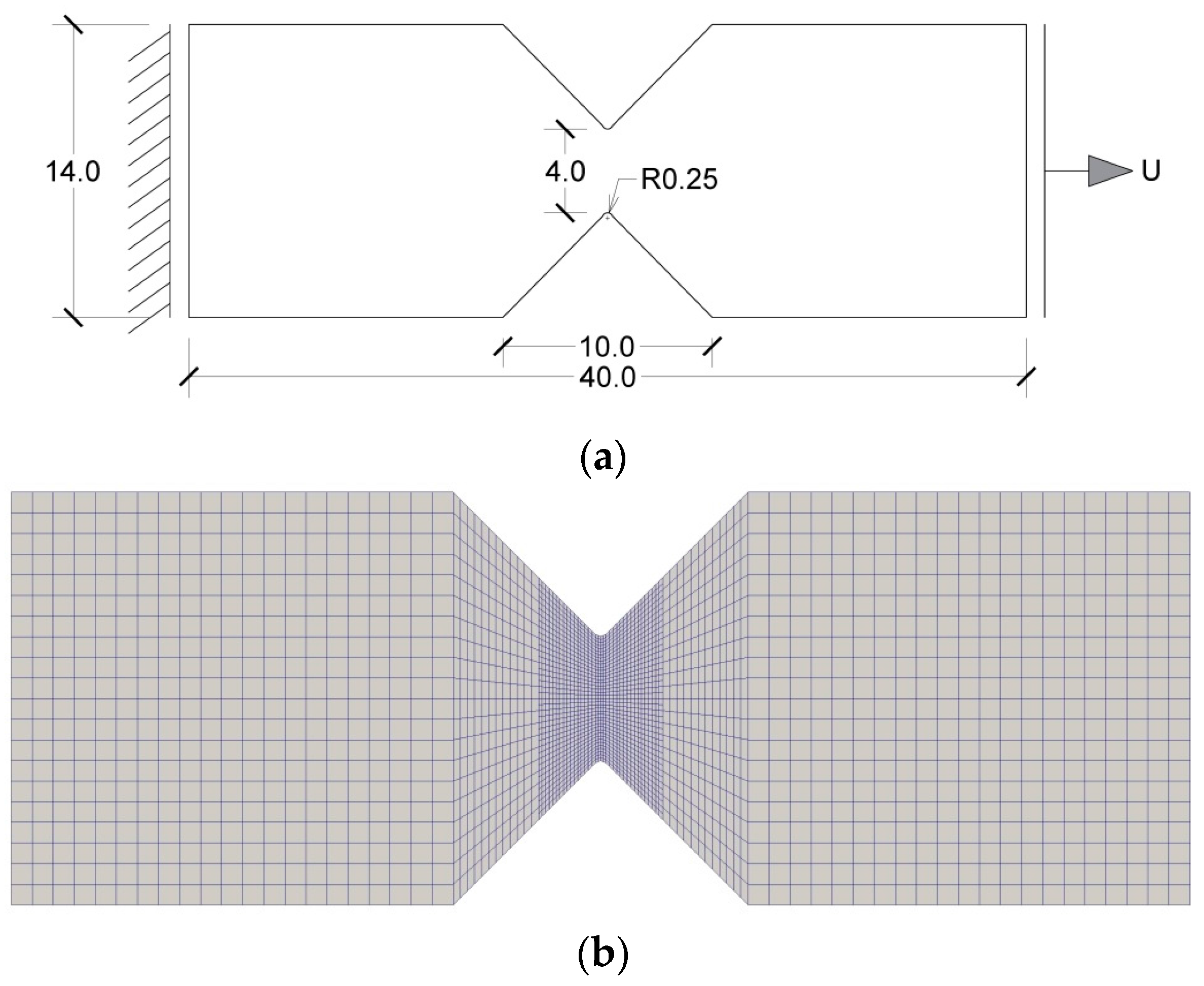
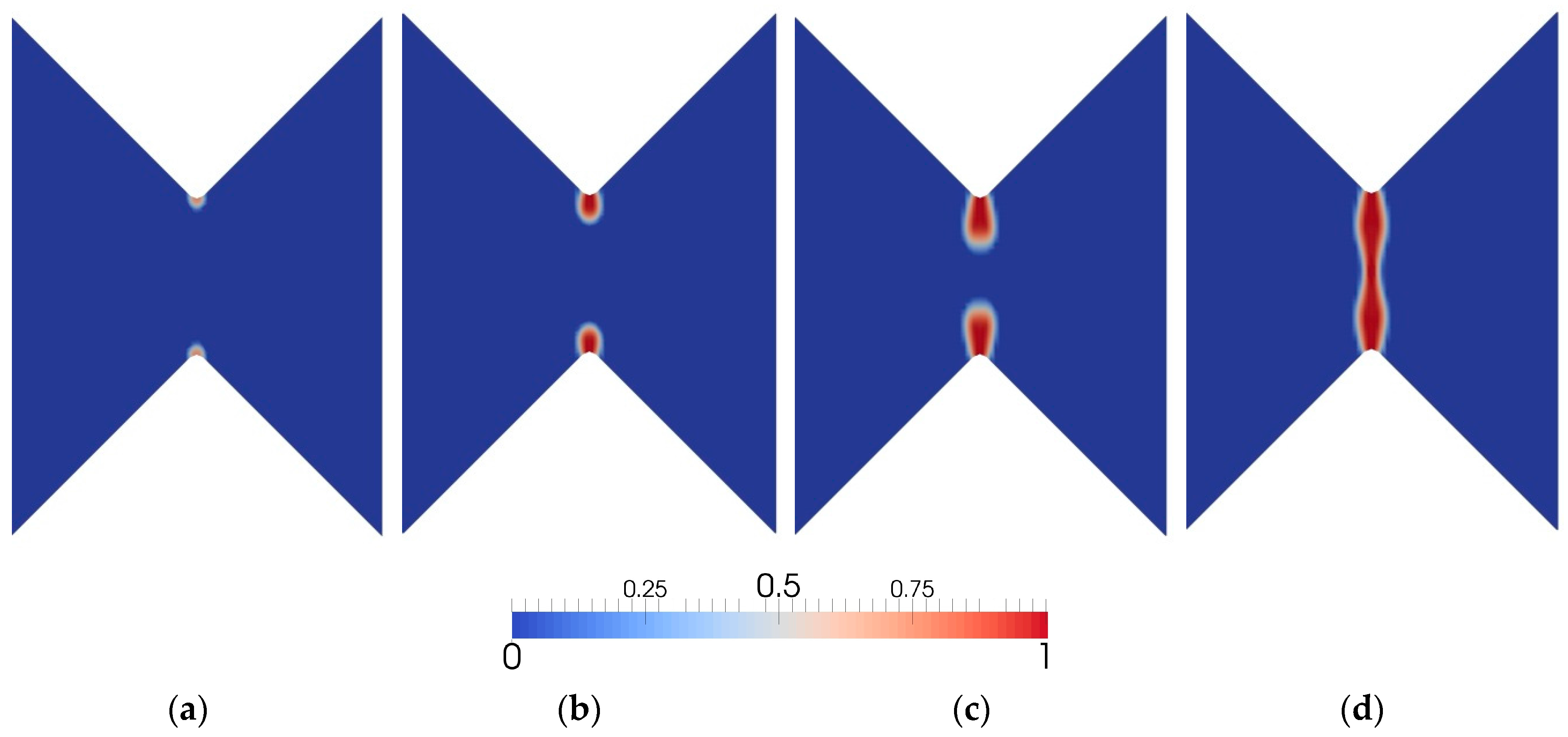
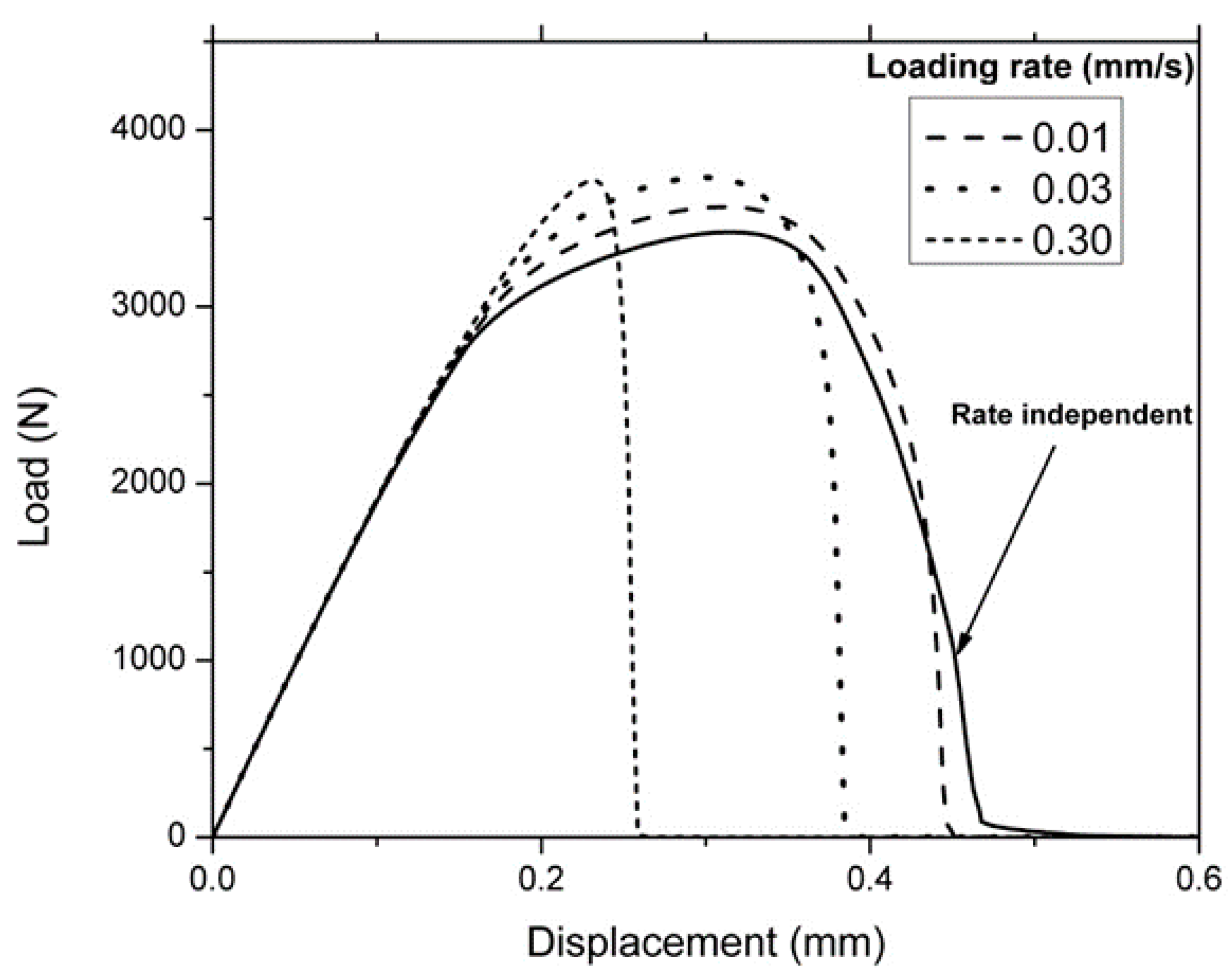
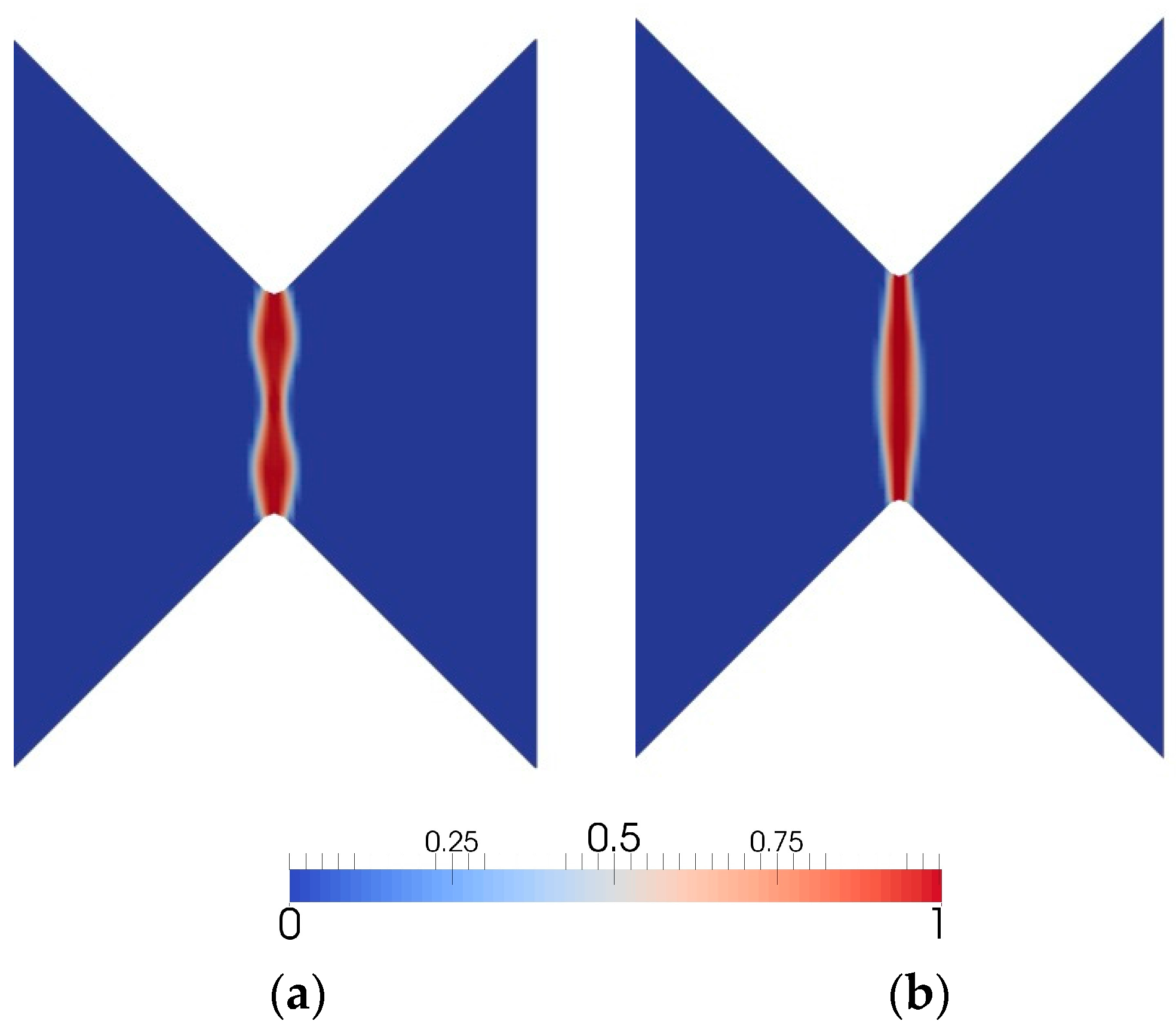
3.2. V-Notched Sample

In two-dimensional simulations, four nodes elements are used in which each node has two degrees of freedom of displacement and one degree of freedom of phase field. As the phase field models require dense mesh within the area of the crack growth, and as the “deal.II” FE code has the ability of the creation and managing the hanging nodes, in developed simulations, meshes are locally refined in the area that the propagation of the cracks are predictable.
In this section, the response of the V-notched specimen is investigated for two cases of rate-independent and rate-dependent. This specimen, which was presented by Miehe et al. [18], is used to verify the proposed model to show the ability to predict the ductile crack propagation for phase field rate-independent model. Geometry and boundary conditions of the V-notched specimen is demonstrated in Figure 3a. The notched geometry leads to a non-uniform stress state on the area near to the notches. This allows us to investigate the effect complex stress state on the model response. Figure 3b shows the meshing structure of the specimen. It can be seen that elements are much finer around the notch, so that the effective element size in this area is 0.139 mm.
For this sample, first, the influence of the loading rate has eliminated by making the rate sensitivity parameter zero. Parameters of the model are shown in Table 2 (physical coefficients are directly acquired from Lie et al. [42]). The resulting force displacement response obtained from the rate-independent model is compared with those presented by Miehe et al. [18] and Lie et al. [42] (Figure 4). The good agreement between the results verifies the accuracy of the model. Furthermore, the process of the crack propagation in rate-independent simulation is shown in Figure 5, through different steps of the loading process.
The impact of the loading rate is also examined for this specimen. To this aim, four different loading rates are used. The obtained force displacement responses in different loading rates are depicted in Figure 6. It is obvious that the level of the force has become greater by increasing the loading rate and the material ductility has reduced. Hence, in a larger loading rate, the material has met the plastic work threshold more quickly so that the crack initiates at a lower displacement. It shows that by increasing the loading rate, the model well represents the physical behavior of material in gradual changing from ductile behavior to brittle one. In Figure 7, the distribution of the phase field variable for rate-independent model is compared with a rate-dependent case at a moderate loading rate. In this figure, by quantitative shrinking of the crack propagation area, the material behavior changes from ductile phase to quasi-brittle which is caused by increasing of the loading rate.

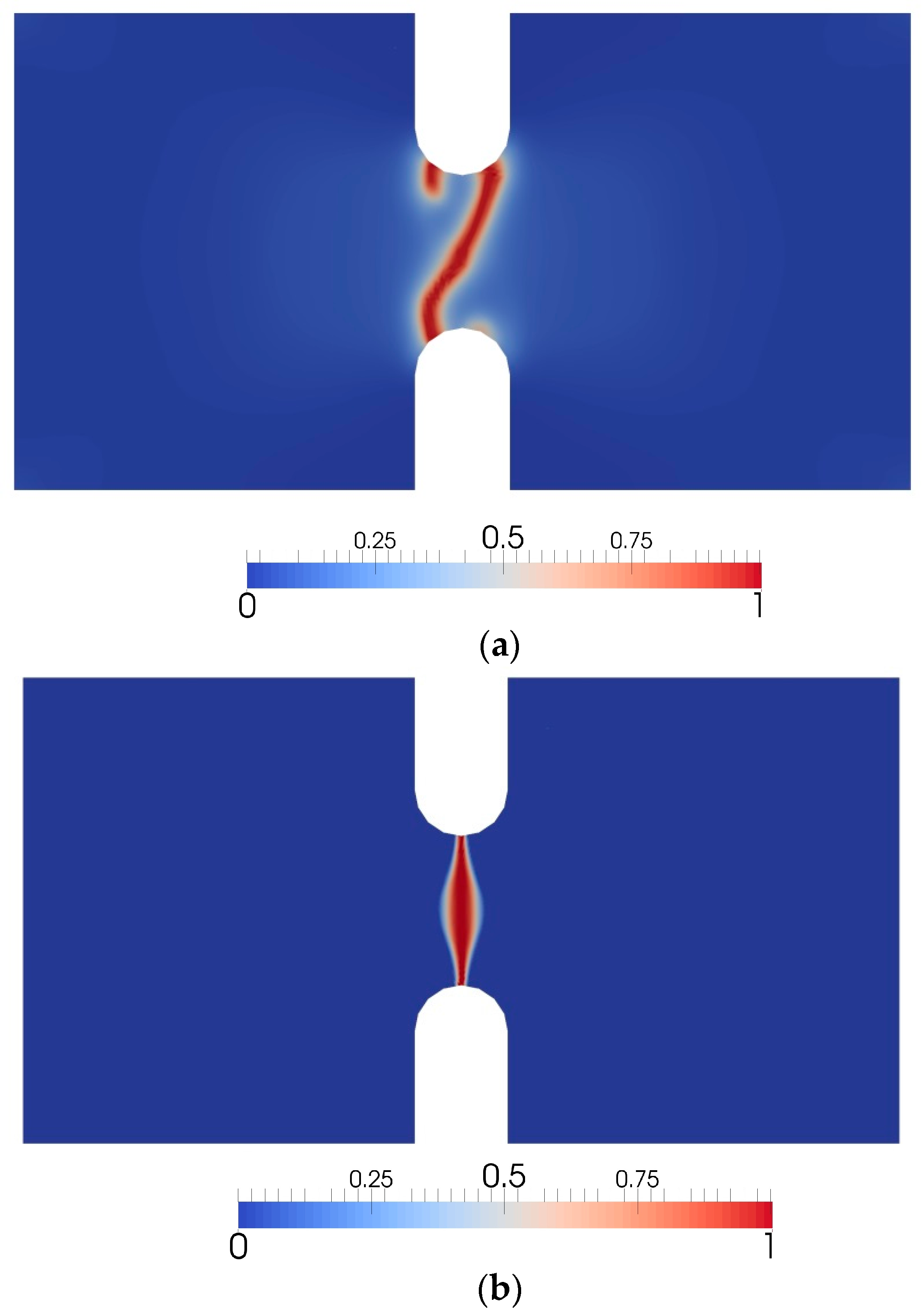
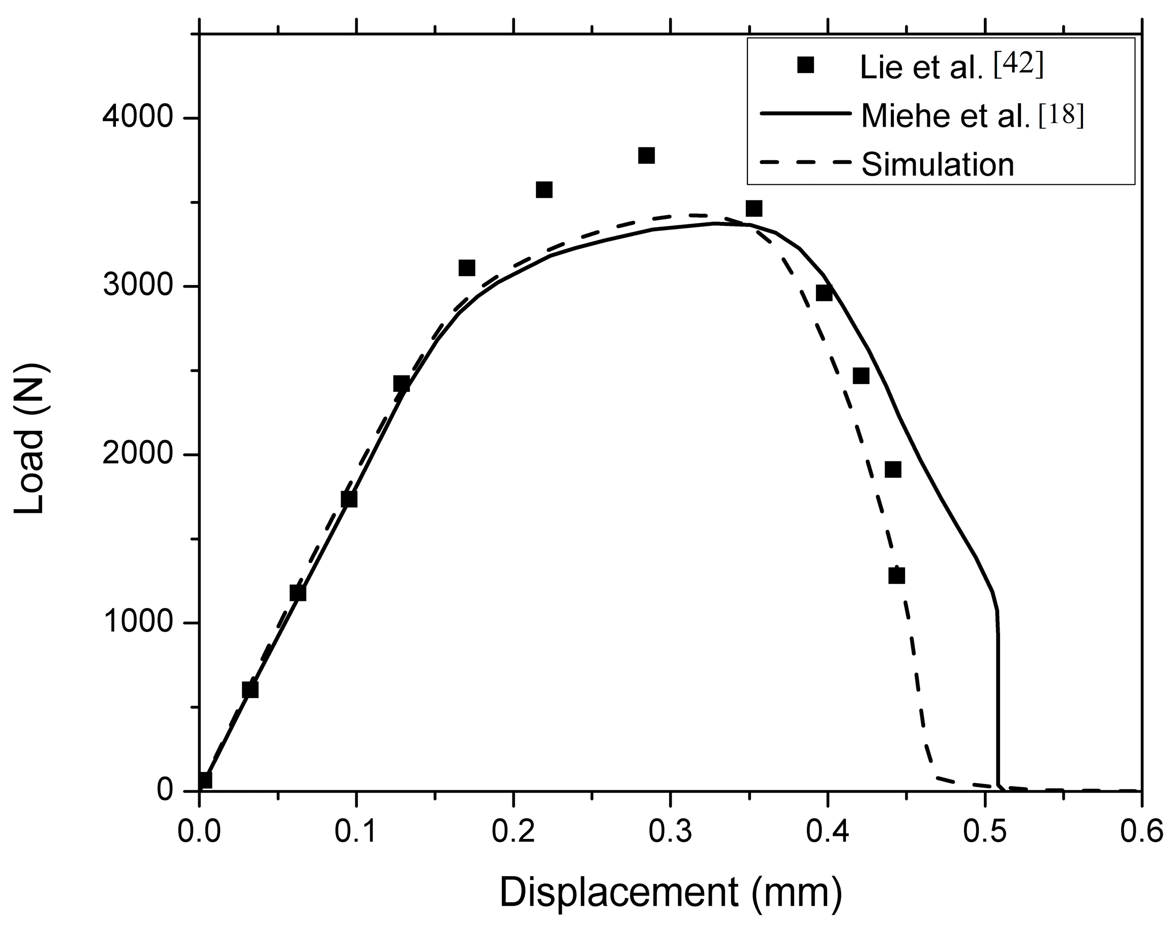
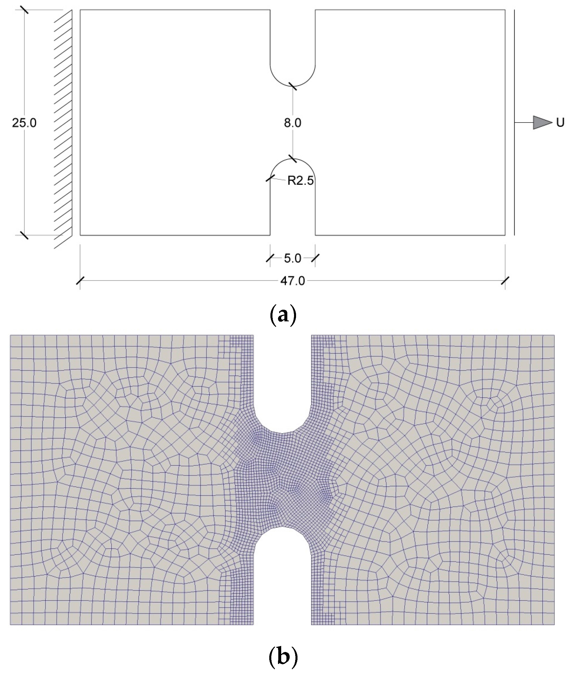
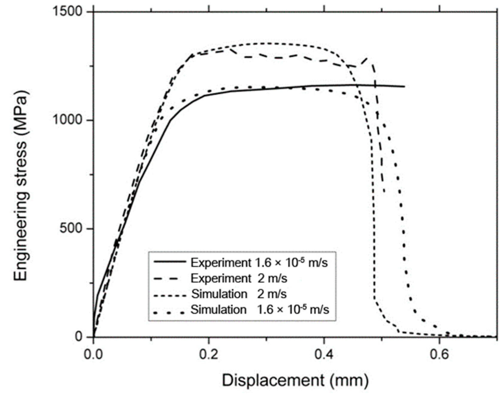
3.3. U-Notched Sample

The aim of this simulation is to, qualitatively and quantitatively, investigate the influence of the loading rate on the fracture process and ductile crack growth and to verify the results, in presence of the loading rate influence. To this aim, the experimental results presented by previous researchers are used. Verleysen and Peirs [43] have experimentally evaluated the effect of the loading rate on the response of the specimens made of Titanium alloy. In one case, they have investigated the behavior of a plane strain U-notched specimen subjected to different loading rates. In this section, this specimen is simulated using our proposed model. The sample geometry and boundary conditions are demonstrated in Figure 8a. The left boundary is constrained, and the displacement is applied on the right side boundary. Moreover, Figure 8b shows the utilized finite element discretization in which the element effective size at the center (based on knowledge of the expected crack path) of the specimen is 0.248 mm. Table 3 shows the parameters used in this simulation.
In Figure 9, the load displacement results obtained from two loading rates are compared with the corresponding experimental data. There is a good agreement between the results. By increasing the loading rate, stress level has increased, and the material fracture has become quicker. In the other word, by increasing the loading rate, the ductility of the material has reduced, and the influence of the brittle crack propagation has increased which is in agreement with the physics of the problem. The distributions of the phase field variable in high and low rates are compared, at the end of the loading process (Figure 10). In the low rate, the pattern of the crack propagation is similar to ones presented by Ambati et al. [15] for a specimen with a similar symmetric notch. It is apparent that by increasing the loading rate, the pattern of the crack propagation has become closer to the pattern of the brittle crack propagation, which is in a good agreement with the patterns presented by Verleysen and Peirs [43], in the high loading rate. Results obtained from this simulation verifies that the accuracy of the model and proves that its numerical solution has the ability of accurate prediction of the influences of loading rate on the physical behavior of the specimens with complex behaviors.

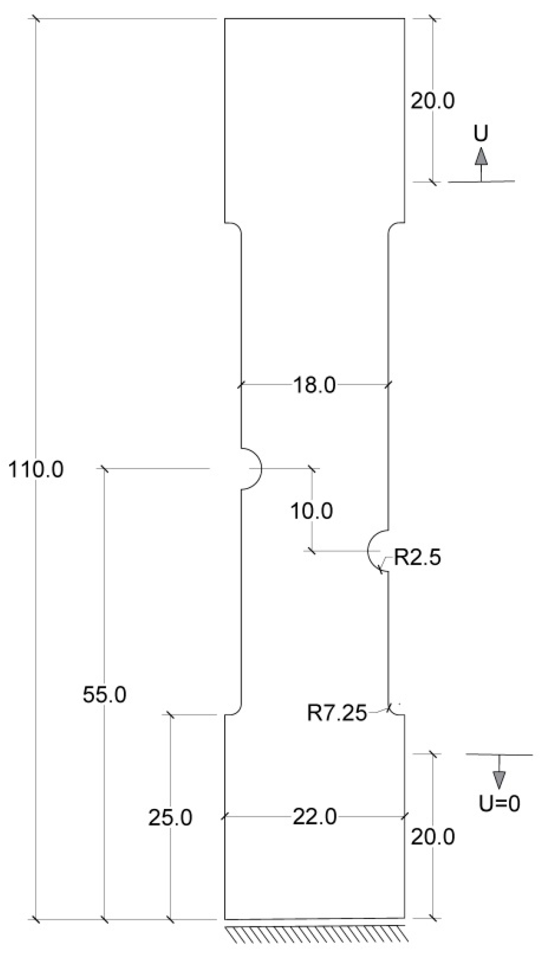
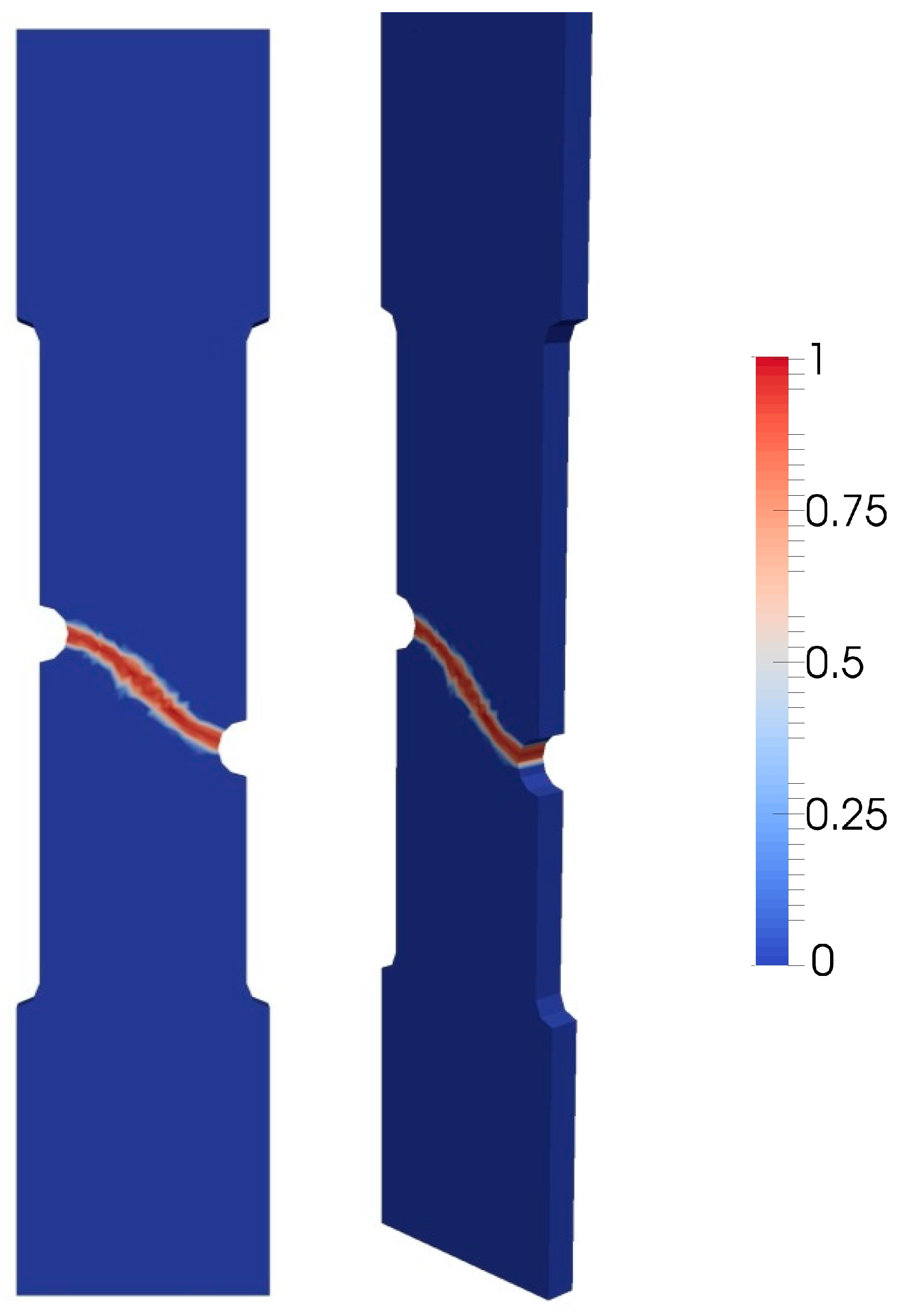
3.4. Three-Dimensional Asymmetric Notched Sample

The aim of this simulation is to evaluate the ability of the model in predicting the crack propagation in a three-dimensional solid, and to validate the model based on the results of the experimental test conducted by other researchers. Hence, a specimen with asymmetric notches is simulated. The result of the experimental test conducted by Ambati et al. [15] is used in which the specimen is made of Al–5005 Aluminum alloy. Figure 11 shows the geometry and the boundary conditions of the specimen. The bottom surface of the specimen is prescribed in all three directions, and the top surface of the specimen is subjected to loading rate of 0.5 mm/min, as prescribed in the experimental test. In this simulation, fully integrated eight-node hexahedral elements are used. The effective size of the elements within the area of crack propagation is 0.988 mm. The material properties of the specimen are presented in Table 4. The final shape of the crack is shown in two different views using the phase field variable contour (Figure 12). The force-displacement graph is compared with the one presented in experimental test (Figure 13). The predicted path of the crack is in a good agreement with the experimental one as well as the force displacement graph. Crack well follows the path between two notches with the angle of 45 degrees. Results verify that the model is able to precisely simulate complex crack propagation patterns in presence of the loading rate effect.

4. Conclusions

In this work, a phase field model for rate-dependent ductile fracture is introduced; to accomplish this goal, a viscoplastic model is coupled with phase field. The total energy function was defined in terms of the energy dissipation caused by plasticity and fracture and the elastic energy. Also, the variational method to ductile fracture, which includes a minimization of the total energy function, was described. In addition, the balance laws for the defined coupled phase field displacement problem were extracted. Moreover, the process of the finite element solution and the numerical integration algorithm was presented based on the return mapping method. Results proved that the model has good ability to predict the path of the crack caused by rate-dependent plastic deformation. Furthermore, proposed model can easily be converted to the standard rate-independent model. The model was validated in comparison with the experimental tests presented in previous studies. The results obtained from the simulations are in a good agreement with the existing experimental results. The influence of the loading rate on the stress response, and gradual changing of the fracture from ductile to the brittle one, caused by increasing the loading rate, was well demonstrated. The results of the one-dimensional simulation precisely determined the impact of the plastic work threshold, rate sensitivity parameter and loading rate on the stress-strain response in the presence of the ductile fracture. Furthermore, similar influences on the force-displacement responses and the distribution of the phase field variable were showed in two- and three-dimensional cases. The suggested model can be developed by considering the influences of different parameters such as the large deformations, kinematic hardening, and various yielding surfaces.

Author Contributions

Hojjat Badnava, Elahe Etemadi and Mohammed A. Msekh contributed to the theoretical parts, including deriving the equations, the simulation process, and the writing of the manuscript. Hojjat Badnava, as the supervisor of this project, managed this study.

Conflicts of Interest

The authors declare no conflict of interest.

References

  1. Kuhn, C.; Müller, R. A continuum phase field model for fracture. Eng. Fract. Mech. 2010, 77, 3625–3634. [Google Scholar] [CrossRef]
  2. Miehe, C.; Hofacker, M.; Welschinger, F. A phase field model for rate-independent crack propagation: Robust algorithmic implementation based on operator splits. Comput. Methods Appl. Mech. Eng. 2010, 199, 2765–2778. [Google Scholar] [CrossRef]
  3. Miehe, C.; Welschinger, F.; Hofacker, M. Thermodynamically consistent phase-field models of fracture: Variational principles and multi-field FE implementations. Int. J. Numer. Methods Eng. 2010, 83, 1273–1311. [Google Scholar] [CrossRef]
  4. Miehe, C.; Schänzel, L.M. Phase field modeling of fracture in rubbery polymers. Part І: Finite elasticity coupled with brittle failure. J. Mech. Phys. Solids 2014, 65, 93–113. [Google Scholar] [CrossRef]
  5. Hofacker, M.; Miehe, C. Continuum phase field modeling of dynamic fracture: Variational principles and staggered FE implementation. Int. J. Fract. 2012, 178, 113–129. [Google Scholar] [CrossRef]
  6. May, S.; Vignollet, J.; de Borst, R. A numerical assessment of phase-field models for brittle and cohesive fracture: Γ-convergence and stress oscillations. Eur. J. Mech. A Solids 2015, 52, 72–84. [Google Scholar] [CrossRef]
  7. Msekh, M.A.; Sargado, J.M.; Jamshidian, M.; Areias, P.M.; Rabczuk, T. Abaqus implementation of phase-field model for brittle fracture. Comput. Mater. Sci. 2015, 96, 472–484. [Google Scholar] [CrossRef]
  8. Msekh, M.A.; Silani, M.; Jamshidian, M.; Areias, P.; Zhuang, X.; Zi, G.; He, P.; Rabczuk, T. Predictions of J integral and tensile strength of clay/epoxy nanocomposites material using phase field model. Compos. Part B Eng. 2016, 93, 97–114. [Google Scholar] [CrossRef]
  9. Liu, G.; Li, Q.; Msekh, M.A.; Zuo, Z. Abaqus implementation of monolithic and staggered schemes for quasi-static and dynamic fracture phase-field model. Comput. Mater. Sci. 2016, 121, 35–47. [Google Scholar] [CrossRef]
  10. Bourdin, B.; Francfort, G.A.; Marigo, J.J. The variational approach to fracture. J. Elast. 2008, 91, 5–148. [Google Scholar] [CrossRef]
  11. Borden, M.J.; Verhoosel, C.V.; Scott, M.A.; Hughes, T.J.R.; Landis, C.M. A phase-field description of dynamic brittle fracture. Comput. Methods Appl. Mech. Eng. 2012, 217–220, 77–95. [Google Scholar] [CrossRef]
  12. Ambati, M.; Gerasimov, T.; Lorenzis, L. A review on phase-field models of brittle fracture and a new fast hybrid formulation. Comput. Mech. 2015, 55, 383–405. [Google Scholar] [CrossRef]
  13. Ambati, M.; Gerasimov, T.; De Lorenzis, L. Phase-field modeling of ductile fracture. Comput. Mech. 2015, 55, 1017–1040. [Google Scholar] [CrossRef]
  14. Ambati, M.; De Lorenzis, L. Phase-field modeling of brittle and ductile fracture in shells with isogeometric nurbs-based solid-shell elements. Comput. Methods Appl. Mech. Eng. 2016, 312, 351–373. [Google Scholar] [CrossRef]
  15. Ambati, M.; Kruse, R.; De Lorenzis, L. A phase-field model for ductile fracture at finite strains and its experimental verification. Comput. Mech. 2016, 57, 149–167. [Google Scholar] [CrossRef]
  16. Duda, F.P.; Ciarbonetti, A.; Sánchez, P.J.; Huespe, A.E. A phase-field/gradient damage model for brittle fracture in elastic–plastic solids. Int. J. Plast. 2015, 65, 269–296. [Google Scholar] [CrossRef]
  17. Miehe, C.; Hofacker, M.; Schänzel, L.M.; Aldakheel, F. Phase field modeling of fracture in multi-physics problems. Part II. Coupled brittle-to-ductile failure criteria and crack propagation in thermo-elastic–plastic solids. Comput. Methods Appl. Mech. Eng. 2015, 294, 486–522. [Google Scholar] [CrossRef]
  18. Miehe, C.; Aldakheel, F.; Raina, A. Phase field modeling of ductile fracture at finite strains: A variational gradient-extended plasticity-damage theory. Int. J. Plast. 2016, 84, 1–32. [Google Scholar] [CrossRef]
  19. Miehe, C.; Kienle, D.; Aldakheel, F.; Teichtmeister, S. Phase field modeling of fracture in porous plasticity: A variational gradient-extended eulerian framework for the macroscopic analysis of ductile failure. Comput. Methods Appl. Mech. Eng. 2016, 312, 3–50. [Google Scholar] [CrossRef]
  20. Hernandez Padilla, C.A.; Markert, B. A coupled ductile fracture phase-field model for crystal plasticity. Contin. Mech. Thermodyn. 2015. [Google Scholar] [CrossRef]
  21. Borden, M.J.; Hughes, T.J.R.; Landis, C.M.; Anvari, A.; Lee, I.J. A phase-field formulation for fracture in ductile materials: Finite deformation balance law derivation, plastic degradation, and stress triaxiality effects. Comput. Methods Appl. Mech. Eng. 2016, 312, 130–166. [Google Scholar] [CrossRef]
  22. Clayton, J.D.; Knap, J. Phase-field analysis of fracture-induced twinning in single crystals. Acta Mater. 2013, 61, 5341–5353. [Google Scholar] [CrossRef]
  23. Clayton, J.D.; Knap, J. Phase field modeling of directional fracture in anisotropic polycrystals. Comput. Mater. Sci. 2015, 98, 158–169. [Google Scholar] [CrossRef]
  24. Clayton, J.D.; Knap, J. Nonlinear phase field theory for fracture and twinning with analysis of simple shear. Philos. Mag. 2015, 95, 2661–2696. [Google Scholar] [CrossRef]
  25. Clayton, J.D.; Knap, J. Phase field modeling and simulation of coupled fracture and twinning in single crystals and polycrystals. Comput. Methods Appl. Mech. Eng. 2016, 312, 447–467. [Google Scholar] [CrossRef]
  26. Areias, P.; Rabczuk, T.; Msekh, M. Phase-field analysis of finite-strain plates and shells including element subdivision. Comput. Methods Appl. Mech. Eng. 2016, 312, 322–350. [Google Scholar] [CrossRef]
  27. Areias, P.; Samaniego, E.; Rabczuk, T. A staggered approach for the coupling of Cahn–Hilliard type diffusion and finite strain elasticity. Comput. Mech. 2016, 57, 339–351. [Google Scholar] [CrossRef]
  28. Shanthraj, P.; Sharma, L.; Svendsen, B.; Roters, F.; Raabe, D. A phase field model for damage in elasto-viscoplastic materials. Comput. Methods Appl. Mech. Eng. 2016, 312, 167–185. [Google Scholar] [CrossRef]
  29. Shanthraj, P.; Svendsen, B.; Sharma, L.; Roters, F.; Raabe, D. Elasto-viscoplastic phase field modelling of anisotropic cleavage fracture. J. Mech. Phys. Solids 2017, 99, 19–34. [Google Scholar] [CrossRef]
  30. Perzyna, P. Fundamental problems in viscoplasticity. Adv. Appl. Mech. 1966, 9, 243–377. [Google Scholar]
  31. Perić, D. On a class of constitutive equations in viscoplasticity: Formulation and computational issues. Int. J. Numer. Methods Eng. 1993, 36, 1365–1393. [Google Scholar] [CrossRef]
  32. Neto, E.A.S.; Peric, D.; Owen, D.R.J. Computational Methods for Plasticity: Theory and Applications; Wiley: Chichester, UK, 2008. [Google Scholar]
  33. Badnava, H.; Mashayekhi, M.; Kadkhodaei, M. An anisotropic gradient damage model based on microplane theory. Int. J. Damage Mech. 2015, 3, 336–357. [Google Scholar] [CrossRef]
  34. Badnava, H.; Kadkhodaei, M.; Mashayekhi, M. A non-local implicit gradient-enhanced model for unstable behaviors of pseudoelastic shape memory alloys in tensile loading. Int. J. Solids Struct. 2014, 51, 4015–4025. [Google Scholar] [CrossRef]
  35. Badnava, H.; Kadkhodaei, M.; Mashayekhi, M. Modeling of unstable behaviors of shape memory alloys during localization and propagation of phase transformation using a gradient-enhanced model. J. Intell. Mater. Syst. Struct. 2015, 18, 2531–2546. [Google Scholar] [CrossRef]
  36. Areias, P.; Msekh, M.A.; Rabczuk, T. Damage and fracture algorithm using the screened poisson equation and local remeshing. Eng. Fract. Mech. 2016, 158, 116–143. [Google Scholar] [CrossRef]
  37. De Borst, R.; Verhoosel, C.V. Gradient damage vs phase-field approaches for fracture: Similarities and differences. Comput. Methods Appl. Mech. Eng. 2016, 312, 78–94. [Google Scholar] [CrossRef]
  38. Heister, T.; Wheeler, M.F.; Wick, T. A primal-dual active set method and predictor-corrector mesh adaptivity for computing fracture propagation using a phase-field approach. Comput. Methods Appl. Mech. Eng. 2015, 290, 466–495. [Google Scholar] [CrossRef]
  39. Bourdin, B.; Francfort, G.A.; Marigo, J.J. Numerical experiments in revisited brittle fracture. J. Mech. Phys. Solids 2000, 48, 797–826. [Google Scholar] [CrossRef]
  40. Bangerth, W.; Heister, T.; Heltai, L.; Kanschat, G.; Kronbichler, M.; Maier, M.; Turcksin, B.; Young, T.D. The deal.II Library, Version 8.1. Available online: http://arxiv.org/abs/1312.2266v4 (accessed on 7 April 2017).
  41. Bangerth, W.; Heister, T.; Kanschat, G. Deal.II Differential Equations Analysis Library, Technical Reference. Available online: http://www.dealii.org (accessed on 7 April 2017).
  42. Li, H.; Fu, M.W.; Lu, J.; Yang, H. Ductile fracture: Experiments and computations. Int. J. Plast. 2011, 27, 147–180. [Google Scholar] [CrossRef]
  43. Verleysen, P.; Peirs, J. Quasi-static and high strain rate fracture behaviour of Ti6Al4V. Int. J. Impact Eng. 2017. [Google Scholar] [CrossRef]
Figure 1. Stress-strain response using the rate-independent model, μ = 0 for different values of the plastic work threshold.
Metals 07 00180 g001
Figure 2. Stress-strain responses for different loading rates (a) ϵ = 0.1 ; (b) ϵ = 1.0 .
Metals 07 00180 g002
Figure 3. The V-notched plane strain tension test: (a) the geometry and associated dimensions (in mm) and (b) the finite element discretization.
Metals 07 00180 g003
Figure 4. Contours of the phase field variable on V-notched sample at different loading stages: (a) 0.37 mm; (b) 0.41 mm; (c) 0.47 mm; and (d) 0.6 mm.
Metals 07 00180 g004
Figure 5. Rate-independent load displacement responses for the V-notched sample in tension.
Metals 07 00180 g005
Figure 6. Effect of loading rate on the load displacement response for the V-notched sample in tension.
Metals 07 00180 g006
Figure 7. Final pattern of the phase field variable for the V-notch sample at different loading rates; (a) rate-independent (b) loading rate 0.03 mm/s.
Metals 07 00180 g007
Figure 8. The U-notched plane strain sample: (a) the geometry and associated dimensions in mm and (b) the finite element discretization.
Metals 07 00180 g008
Figure 9. The U-notched plane strain sample. Effect of the loading rate on the model response. Experimental data by Verleysen and Peirs [43].
Metals 07 00180 g009
Figure 10. The final phase field distribution of the U-notched plane strain sample at (a) low loading rate and (b) high loading rate.
Metals 07 00180 g010
Figure 11. Sample geometry and boundary conditions.
Metals 07 00180 g011
Figure 12. Contour plots of the phase field for the asymmetric notched sample.
Metals 07 00180 g012
Figure 13. Load–displacement response for the asymmetrically notched sample. Experimental data by Ambati et al. [15].
Metals 07 00180 g013
Table 1. Model parameters for the one-dimensional simulations.
Material ParameterValues
Young’s modulus68.8 (GPa)
Poisson’s ratio0.33
Yield stress ( σ y )320 (MPa)
Hardening modulus655 (MPa)
Fracture energy ( g c )69 (N/mm)
Rate sensitivity ( ϵ )1.0
β p and β e 1.0
Table 2. Model parameters for the V-notched sample of Al-alloy 6061 material.
Material ParameterValues
Young’s modulus68.9 (GPa)
Poisson’s ratio0.33
Yield stress ( σ y )475 (MPa)
Hardening modulus561 (MPa)
Fracture energy ( g c )18 (N/mm)
Length scale (L)0.28 (mm)
Rate sensitivity ( ϵ )0.6
Viscosity ( μ )10 (s)
Plastic work threshold ( W c )120.0 (MPa)
β p and β e 1.0
Table 3. Model parameters for the Ti6Al4V U-notched sample.
Material ParameterValues
Shear modulus (G)80.8 (GPa)
Poisson’s ratio0.3
Yield stress ( σ y )780 (MPa)
Hardening modulus40 (MPa)
Fracture energy ( g c )23 (N/mm)
Length scale (L)0.50 (mm)
Rate sensitivity ( ϵ )0.06
Viscosity ( μ )2 (s)
Plastic work threshold ( W c )139.0 (MPa)
β p and β e 1.0
Table 4. Model parameters for the Al–5005 asymmetric notched sample.
Material ParameterValues
Young’s modulus70.9 (GPa)
Poisson’s ratio0.34
Yield stress ( σ y )125 (MPa)
Hardening modulus28 (MPa)
Fracture energy ( g c )35 (N/mm)
Length scale (L)1.98 (mm)
Rate sensitivity ( ϵ )0.5
Viscosity ( μ )5 (s)
Plastic work threshold ( W c )30.0 (MPa)
β p and β e 1.0

